


Abstract
Efficient tractor coverage planning requires suitable swath orientations and kinematically feasible connections. In two-pass diagonal harrowing, sequential boustrophedon planning treats the two swath families independently and may introduce avoidable connection travel. This study proposes a Field-Geometry-Aware Bidirectional Coverage and Connection Path Co-Optimization algorithm (FG-BCO) for a single tractor operating in convex, obstacle-free polygonal fields. FG-BCO clips two parallel swath families to the field boundary, constructs feasible cross-pass links between oriented endpoints, assembles alternating route paths, and applies subset dynamic programming to optimize their visiting order and traversal orientation. The resulting route is converted into a forward-only trajectory and checked against boundary-containment and minimum-turning-radius constraints. FG-BCO was compared with Sequential Boustrophedon Coverage Path Planning (SB-CPP) in rectangular, regular pentagonal, regular hexagonal, and irregular fields using 648 matched angle pairs per field. When the minimum path length of each algorithm was selected independently from the tested angle pairs, FG-BCO achieved reductions of 18.65%, 9.65%, 15.20%, and 17.11% in the four fields, respectively. However, FG-BCO produced shorter routes in only 57.87%, 41.82%, 40.43%, and 40.59% of the matched cases. The corresponding mean paired saving rates were 0.646%, −0.484%, −0.144%, and −0.833%, with medians of 0.939%, −1.060%, −0.923%, and −1.094%. These results distinguish the potential reduction obtainable through angle selection from performance under an arbitrary prescribed angle pair. FG-BCO is advantageous when the two swath families produce favorable endpoint proximity, heading compatibility, and turning space, but its improvement is not universal. Preliminary evaluation of the working-angle pair in relation to the target field geometry is therefore recommended before application.
1. Introduction
Complete Coverage Path Planning (CCPP) is a fundamental operational challenge that is critical for precision agriculture and the deployment of unmanned agricultural tractors (UATs), particularly concerning resource utilization, operational efficiency, and sustainable farm management [1,2,3]. The automated navigation and auto-steering of various agricultural systems—ranging from tillage to harvesting—induce complex path tracking dynamics and pass-to-pass accuracy requirements [4,5]. A recent systematic review further classified agricultural robot navigation research into global planning, local planning, multi-robot cooperative planning, and trajectory tracking control [6]. Recently, autonomous field operations have garnered significant attention, as redundant overlapping, unworked gaps, and excessive headland turns exert tremendous energy consumption and threaten the economic efficiency of the entire agricultural production system [7,8].
Historically, foundational studies have focused on canonical region decomposition and basic Sequential Boustrophedon patterns to understand traversal mechanisms and optimize driving sequences. For standard 2D planar fields, exact cellular decomposition and heuristic models have detailed sub-region generation, driving direction determination, and generic benchmarking frameworks [9,10]. Evolution-based and meta-heuristic theories have been extensively developed to predict optimal routing and minimize headland distances, employing Markov chain improved Genetic Algorithms (GA) and Estimation of Distribution Algorithms (EDA) [11,12]. At the local-planning level, an improved A* method combined with Bezier-curve post-processing has been proposed to enhance obstacle-avoidance path smoothness for agricultural mobile robots [13]. Furthermore, studies have evaluated complex field constraints such as obstacle avoidance using Bezier curves [14] and chance-constrained programming [15], heuristic cooperative planning for multi-machine dependent tasks [16,17], and precedence provisions in disjoint regions using Mixed Integer Linear Programming (MILP) [18]. Specific applications, such as hybrid ant colony optimization for 3D point cloud maps in horticultural pruning, have also broadened the understanding of intelligent spatial planning [19]. Coverage planning has also been extended to heterogeneous UAV groups in precision agriculture, where genetic-algorithm-based optimization was used to select the operating UAV subset and reduce flight cost [20]. Within ground agricultural operations, offline multi-robot planning has been studied for paddy-field weeding, while hierarchical multi-region methods have combined collision-free path generation with task-sequence optimization [21,22].
The turning dynamics and kinematic constraints of agricultural vehicles have also been thoroughly investigated, addressing specific physical parameters such as continuous curvature and minimum turning radii [23]. To accurately capture traversal trajectories without kinematic violations, advanced approaches including Dubins path modeling and generalized traveling salesman problem (GTSP) formulations have been employed [24]. With the advancement of intelligent navigation, the research focus has shifted toward complex terrain adaptations and fully automated field operations. For instance, customized cost functions and region decomposition methods have been utilized to evaluate 3D coverage paths on hilly terrains to minimize energy consumption [25,26]. Moreover, complete paddy field-coverage planners have been successfully implemented to simulate inner and outer-work paths, along with complex boundary corner turning methods for fully autonomous tillage and puddling tractors [27,28].
Existing studies have advanced agricultural coverage planning through region decomposition, working-direction optimization, and curvature-constrained routing. Yang et al. investigated the coordinated selection of region segmentation and working directions [9], while Höffmann et al. formulated cell sequencing and entry–exit selection as a generalized traveling salesman problem [23]. In two-pass diagonal harrowing, the spatial relationship between two swath families introduces an additional routing consideration. Completing the two passes sequentially restricts the available connections to those within each pass and a transfer between them. Allowing working segments from different passes to be visited in an interleaved sequence provides additional connection choices whose usefulness depends on the alignment of the swath endpoints with the field boundary.
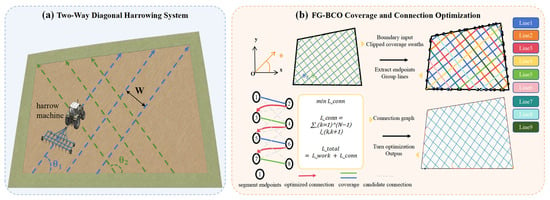
This study develops a Field-Geometry-Aware Bidirectional Coverage and Connection Path Co-Optimization algorithm to incorporate these cross-pass connection choices into route planning. For a prescribed pair of working orientations, two swath families are generated and clipped to the field boundary. An endpoint connection graph is then constructed using boundary distance, endpoint proximity, and heading compatibility to assemble alternating route paths from the two families. These route paths serve as the units for jointly optimizing their visiting order and traversal orientations. This formulation couples the organization of the two passes at the working-segment level with connection optimization at the route-path level. The resulting route is subsequently processed for turn generation and checked against the prescribed turning-radius and boundary-containment constraints. Figure 1 illustrates the autonomous two-pass diagonal harrowing system and the main stages of the proposed FG-BCO framework.
Figure 1.
Overall framework of the proposed study. (a) Schematic of the autonomous two-pass diagonal harrowing system, showing the two working directions θ1 and θ2, and the implement width W. (b) Main procedure of FG-BCO, including boundary-clipped swath generation, endpoint extraction, connection-graph construction, route-path ordering, and turn-constrained trajectory generation.
The proposed framework enables the traversal sequence to adapt to the endpoint configuration of both swath families, linking field geometry with cross-pass route organization. Its performance is evaluated against sequential boustrophedon planning over a full-factorial matrix of working-angle pairs in rectangular, regular pentagonal, and regular hexagonal fields. An additional case study uses an irregular field boundary derived from measured data, simplified to 25 vertices, and uniformly scaled to an area of 60,000 m2. The evaluation compares total path length, while representative trajectories illustrate the differences in route organization. All-path swept-area coverage is assessed using a grid-based metric, and computational runtime and memory usage are compared across the four fields. Table 1 summarizes the planning characteristics and scope of representative coverage methods in relation to FG-BCO.
Table 1.
Planning formulations and coverage organization of representative methods.
2. Materials and Methods
2.1. Problem Definition and Modeling Assumptions
This study considers two-pass diagonal harrowing performed by a single unmanned agricultural tractor on a planar field. The field is represented by a convex polygon Ω in a two-dimensional Cartesian coordinate system. The symbol ∂ is the boundary operator; therefore, ∂Ω denotes the polygonal boundary of the field. The field contains no internal obstacles or subfield divisions.
The polygon is preprocessed before path generation. Duplicate vertices are removed, and clockwise vertex sequences are converted to counterclockwise order. Nearly collinear vertices are merged to avoid very short boundary edges. A polygon is rejected if its boundary contains self-intersections. Terrain slope, soil resistance, wheel slip, travel speed, and interactions between multiple machines are not considered. These assumptions allow the analysis to focus on field geometry, coverage direction, and path connection. In practical field operation, the feasibility of a harrowing route depends on more than the implement width and the minimum turning radius. Other relevant parameters include the length and width of the tractor–implement system, the implement overhang and swept envelope, the available headland width, the lateral boundary clearance, positioning uncertainty, the field entrance location, and any prescribed terminal condition. Terrain slope, soil-dependent wheel slip, operating speed, and tractor–implement articulation may further affect tracking accuracy and maneuverability. The present study focuses on the upper-level geometric planning problem. Although the implementation permits configurable vehicle dimensions and boundary offsets, these constraints were not activated in the controlled benchmark experiments. Dynamic, terrain-dependent, and soil-dependent effects are expected to be handled by the lower-level motion-control and safety systems in future field applications.
The two harrowing passes follow the working orientations θ1 and θ2. Reversing the travel direction along a straight swath does not change its geometric orientation. Therefore, both working orientations are defined within [0°,180°). The second orientation is calculated as
where θ1 and θ2 are the orientations of the first and second swath families, respectively, and Δ is their smaller included angle. The modulo operation returns θ2 to the interval [0°,180°) when θ1 + Δ is equal to or greater than 180°. Equation (1) is used to generate the second working orientation without creating an equivalent direction outside the specified angular range.
θ2 = mod(θ1 + Δ, 180°)
The implement working width is denoted by W, which also defines the nominal spacing between adjacent swaths. The minimum turning radius is denoted by Rmin. Every turn and connection path must satisfy this constraint. The tractor is represented by its centerline, and reverse motion is not allowed. All feasibility checks in this study are therefore performed at the centerline level. Centerline-level geometric feasibility means that the reference-point trajectory stays inside the planning polygon, contains no reverse motion, and respects the minimum turning radius. It does not imply vehicle-level operational feasibility, because the swept footprint of the tractor and implement is not evaluated; a trajectory that is feasible at the centerline level may still place the tractor body or the implement outside the field during a turn.
An externally specified start reference point p0 is used to determine the initial working segment. This reference point may represent a field entrance or the current tractor location and is not required to lie on a generated swath. Among all retained working-segment endpoints, the endpoint with the minimum Euclidean distance to p0 is selected as the actual route start. The associated segment is oriented so that traversal begins at this endpoint, and the route path containing it is fixed as the first path in the subsequent ordering stage. No fixed terminal position or terminal orientation is imposed; the resulting planning problem is therefore formulated as an open route. The boundary offset is set to zero, and the vehicle footprint is not included in the boundary feasibility test. Therefore, working-line endpoints may lie directly on ∂Ω. This setting allows the implement to reach the field edge, but the clearance of the tractor body is not evaluated. For operational deployment, a nonzero lateral safety clearance should be applied between the tractor–implement system and the field boundary. This clearance can be implemented by inwardly offsetting the original field polygon and constraining the vehicle reference point and its swept footprint to remain inside the resulting feasible region. The required offset is machine- and site-specific and should account for the tractor and implement dimensions, positioning error, terrain conditions, boundary type, and the consequences of crossing the field edge. The zero boundary offset adopted in the present simulations is therefore a controlled experimental setting used to isolate the effects of route sequencing and connection optimization; it should not be interpreted as a recommended value for autonomous field operation. In practical deployment, the selection and validation of the safety clearance should follow the applicable risk-assessment and autonomous-operation requirements for agricultural machinery.
The total route contains straight working segments and the connections between them. The connections include turns, links between line chains, and boundary-following transfers. These components may be recorded separately, but the total path length is used as the primary measure of route efficiency. Total path length is a geometric quantity: it does not capture the different speeds and dynamic loads of straight working segments and curved connections, and it is therefore not a direct measure of operating time, energy consumption, soil compaction, or fuel and electric-energy use. Because the implement remains engaged along the entire route, both working and connection travel contribute to the swept area, so connection travel is not purely non-productive in the present setting.
2.2. Field-Geometry-Aware Bidirectional Coverage and Connection Path Co-Optimization
FG-BCO generates the coverage route in four stages. First, two families of parallel swaths are generated and clipped by the field boundary. Second, feasible links are constructed between endpoints from different swath families. These links are used to form alternating route paths. Third, the route paths are ordered and assigned traversal orientations to reduce connection travel. Finally, the resulting polyline is smoothed and checked against the field boundary and the minimum turning radius.
2.2.1. Geometry-Aware Swath Generation
For each harrowing pass, the working orientation is converted into a direction vector and a normal vector:
where k is the pass index and θk is the working orientation of pass k. The vector μk is the unit vector along the working direction, while nk is the corresponding unit normal vector. Equation (2) defines the direction of each swath and the direction in which adjacent swaths are placed.
The field polygon is projected onto nk. The minimum and maximum projected coordinates are denoted by ck,min and ck,max, respectively. These two values define the lateral range of the swath family for pass k. The offset of each parallel line is calculated as
where ck,m is the lateral offset of line m in pass k, m is the line index, and W is the implement working width. The integer Nk is the number of parallel lines generated for pass k. Its value is selected so that every offset satisfies ck,m ≤ ck,max. Equation (3) distributes the parallel lines across the field at the prescribed spacing W.
ck,m = ck,min + mW, m = 0,1,…,Nk − 1
Each offset defines an infinite line. The line is clipped by the field polygon to obtain the corresponding working segment:
where Sk,m is the working segment associated with pass k and line index m. The vector x represents a point in the two-dimensional coordinate system. The expression defines the infinite line at offset ck,m, and its intersection with Ω limits the line to the field interior. Equation (4) therefore ensures that every working segment conforms to the actual polygonal boundary.
Degenerate intersections with negligible length are removed. For each retained segment, the algorithm stores its two endpoints, associated boundary edges, pass index, lateral offset, and length. The endpoint and boundary information is used in the subsequent connection stage. The segments from the two passes are combined into one working-segment set, while their pass identities are retained.
2.2.2. Endpoint Graph and Alternating Route Path Construction
Each working segment can be traversed in two directions. Each direction defines an entry endpoint, an exit endpoint, and the corresponding headings. These oriented segment states form the nodes of the endpoint graph. A directed edge represents a feasible transfer between two segments.
Candidate edges are considered only between segments from different passes. Both the Euclidean endpoint distance and the shortest boundary distance must not exceed the thresholds 8W, which are specified as fixed multiples of the implement width W rather than as independent tuning constants; they therefore scale with the machine configuration instead of being tied to a particular field. The transfer must also be compatible with the exit and entry headings. A connection between nearly opposing segments is rejected when the available endpoint and lateral clearances are smaller than 2Rmin. These criteria restrict the candidate links used to assemble alternating route paths. The resulting route-path set is subsequently passed to the ordering stage, while the final connections remain subject to turn generation and geometric feasibility checks.
The remaining candidate edges are ranked by
where gij is the local connection cost from oriented segment i to oriented segment j. The vectors and are their exit and entry endpoints. is the length of the shorter boundary path between the two endpoints. The term is their Euclidean distance. The weight β is set to 0.25 in all experiments. A lower gij indicates a preferred connection.
The weight was fixed at 0.25 to give greater emphasis to boundary-following distance while retaining endpoint proximity as a secondary consideration. The same value was used for all fields and angle pairs without field-specific tuning. Because changing the weight may alter the ranking of candidate links, its influence on route construction and final path length requires further sensitivity analysis.
Starting from the working-segment endpoint selected using the start reference point P0, FG-BCO repeatedly selects the lowest-cost feasible link to an unused segment. Because each link joins different passes, the resulting sequence alternates between the two swath families. This sequence is defined as a route path.
When no further feasible link is available, a new route path is started from an unused segment. The process continues until all retained segments have been assigned. Isolated corner segments shorter than W are removed unless their removal would eliminate the entire working-segment set.
2.2.3. Global Route-Path Ordering and Orientation
Suppose that the endpoint graph produces Q route paths, denoted by P0,…,PQ−1. Each route path can be traversed in two orientations. The route-ordering stage determines both the visiting order and the traversal orientation of these paths. For route path i in orientation a and route path j in orientation b, the transition cost is
where cij(a,b) is the transition cost from path i to path j, and a,b ∈ {1,2} are their traversal orientations. The function gives the length of the shorter boundary path between the selected exit and entry endpoints. The vectors and are the exit endpoint of path i in orientation a and the entry endpoint of path j in orientation b. The terms pint, phead, and pturn penalize boundary-line intersections, unfavorable headings, and insufficient turning space. The weights are set to λint = 10and λhead = 20.
The weights are set to λint = 10 and λhead = 20, so heading compatibility is penalized more heavily than near-boundary intersection. The intersection penalty is triggered within 2W of the field boundary. The heading penalty is triggered when the transfer angle exceeds 150°. When an opposing transition fails the 2Rmin clearance test, a large turning penalty pturn is applied.
The coefficients in Equations (5) and (6) express the intended balance between connection distance and geometric compatibility. They were specified before the benchmark evaluation and held constant across all tested fields and angle pairs. The distance and clearance thresholds are expressed relative to the implement width and minimum turning radius, whereas the angular thresholds control heading compatibility and the acceptance of connection candidates. These settings can influence candidate selection, route-path assembly, and the resulting connections. A systematic sensitivity analysis is beyond the scope of the present study and is left to future work.
Let π = (π1,…,πQ) be the visiting order and b = (b1,…,bQ) be the corresponding orientation vector. The optimization objective is
where J* is the minimum total transition cost. The index πq identifies the path visited at position q, and bq ∈ {0,1} specifies its orientation. The transition cost is defined in Equation (6). Equation (7) selects the route-path order and orientations with the lowest total cost.
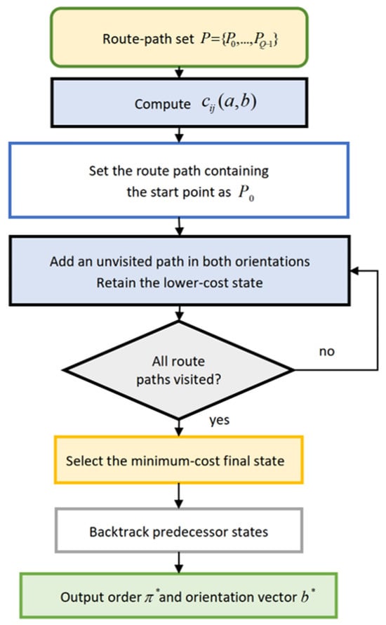
For Q ≤ 20, subset dynamic programming determines the route-path order and traversal orientations. The route path containing the working-segment endpoint selected from the start reference point is fixed as the first path. Each state records the visited route-path subset, the last visited path, and its traversal orientation. The algorithm adds each unvisited path in both orientations and retains the state with the lowest accumulated cost. Once all route paths have been visited, backtracking yields the final order and orientation vector. When the number of route paths exceeds Q > 20, the exponential dynamic-programming stage is skipped and the deterministic order produced by the endpoint-graph construction is retained. This cutoff limits the computational cost of route-path ordering. It leaves the assembled route-path set unchanged but may alter the inter-path connections and the resulting route quality. Regardless of the ordering procedure used, the final route is subjected to the same turn-generation and geometric feasibility checks. The cutoff is introduced because the number of subsets grows as 2Q, making larger exact instances increasingly expensive in both time and memory. The dynamic-programming procedure is illustrated in Figure 2.
Figure 2.
Subset dynamic programming workflow for determining the global route-path order π* and orientation vector b*.
Let N denote the total number of retained working segments, V the number of field-boundary edges, E the number of feasible candidate links, and Q the number of route paths. Swath generation and polygon clipping require O(NV) time. The endpoint-graph stage examines cross-pass segment pairs and has a worst-case time complexity of O(N2V), while sorting the feasible links requires O(ElogE) time. For Q ≤ 20, the subset dynamic program requires O(Q22Q) time and O(Q2Q) memory. When Q > 20, the dynamic-programming stage is omitted, and the computational cost is dominated by endpoint-graph construction and candidate-link sorting. Therefore, the exponential component is applied only to the reduced route-path set rather than directly to all individual working segments.
The route paths generated in the preceding stage remain fixed during ordering optimization. Within the dynamic-programming size limit, the algorithm determines the minimum-cost visiting order and traversal orientations under Equation (6), subject to the prescribed starting condition. This optimum is defined for the assembled route-path set; the working-angle pair and the internal segment sequence of each route path are not decision variables at this stage.
2.2.4. Curvature-Constrained Turn Generation and Validation
The ordered route initially consists of straight working and connection segments. At each junction, the heading change and the available lengths of the adjoining segments are evaluated. Heading changes smaller than 5° are treated as nearly collinear during fillet construction. For other junctions, a circular fillet is attempted subject to the prescribed minimum turning radius and the available segment lengths. An accepted fillet is tangent to both adjoining straight segments and is sampled at an angular interval of 8° for subsequent geometric processing. Junctions that cannot be resolved by this construction are handled by the connection procedures described below.
A connection between two working segments is processed as one unit. When sufficient space is available, its entry and exit corners are smoothed independently. Otherwise, the algorithm first attempts a single circular work-to-work turn. If this construction is infeasible, forward-only Dubins bulb-turn candidates are generated. Bulb-turn generation is restricted to working segments belonging to the same line family, with a directional deviation of less than 10° from parallel or antiparallel alignment and a lateral separation of at least half the implement width. These conditions are used as geometric admissibility tests for bulb-turn candidates. The angular threshold defines the permitted deviation from parallel or antiparallel alignment, while the lateral-separation threshold limits candidate generation to sufficiently separated working segments. The trimming increment and the maximum trimming distance are likewise scaled to the machine configuration: in the present experiments they correspond to 0.5W and 2W, respectively. These limits bound the amount of working-segment shortening during turn insertion. Coverage is evaluated on the resulting route using the metric defined in Section 2.4. Candidates that leave the planning polygon, self-intersect, or produce a nonlocal detour are rejected, and a feasible curve-straight-curve solution is preferred.
After all connection units have been processed, residual short segments and defective connections are repaired when possible. The final route is then checked for boundary containment and minimum-turning-radius compliance. Local turning radii are evaluated at the joins between successive path elements and at any remaining polyline corners. An intermediate construction failure does not invalidate the route if a subsequent repair produces a feasible connection. The route is classified as geometrically feasible at the centerline level only when the reference-point trajectory remains inside the planning polygon, contains no reverse motion, and has no turning-radius violation. This condition applies to the vehicle reference point and does not guarantee that the tractor body or the implement remains inside the field during turns.
2.3. Sequential Boustrophedon Coverage Path Baseline
SB-CPP is adopted as the reference algorithm because it represents the conventional sequential organization of two-pass diagonal harrowing. For each paired test, it receives the same field boundary, working orientations, implement width, minimum turning radius, number of passes, and boundary offset as FG-BCO. Both methods use the same line–polygon intersection procedure to generate the initial working segments and the same routine for turn generation. The comparison therefore evaluates the two route-organization strategies under common initial coverage geometry and geometric constraints.
Within each pass, SB-CPP orders the swaths by lateral offset and traverses successive swaths in alternating directions. All working segments of the first pass are completed before the second pass begins; cross-pass route assembly and global route-path ordering are not performed. Adjacent swaths are connected by same-side turns, while the transfer between passes follows the shorter field-boundary route. Each method retains its own start-selection rule, as described in Section 2.4. Consequently, the comparison concerns the routes generated by the two methods from their respective first working segments, rather than routes with an identical physical starting condition.
2.4. Experimental Design
The evaluation comprised three regular benchmark fields—a rectangle, a regular pentagon, and a regular hexagon—and an additional irregular-field case study. These geometries were selected as controlled test cases rather than as a statistical representation of the frequency of field shapes in agricultural regions. The rectangle provides an idealized baseline with two orthogonal boundary directions and two pairs of parallel edges. The regular pentagon introduces an odd number of sides and no opposite parallel-edge pairs, thereby increasing the mismatch between the prescribed harrowing directions and the field boundary. The regular hexagon contains more boundary transitions and three pairs of opposite parallel sides with different orientations, providing a complementary test of the interaction between swath directions and boundary geometry. The areas of the three regular fields were kept approximately equal so that the influence of boundary geometry could be examined without introducing a substantial difference in field scale. The same implement width, minimum turning radius, boundary offset, and number of passes were used in all simulations. All non-angular algorithm settings were fixed for the benchmark evaluation and applied consistently across the four fields and all tested angle pairs, without field-specific tuning. The two methods share the same machine, smoothing, and trimming parameters, while retaining their respective start-selection rules. These fixed parameters are listed in Table 2, and the corresponding boundary coordinates are provided in Table 3. From an agricultural perspective, these geometries can be regarded as stylized abstractions of regular consolidated fields and multi-edged parcels formed by roads, drainage channels, shelterbelts, and neighboring property boundaries, rather than exact replicas of individual farms. The irregular-field boundary was derived from measured data, simplified to 25 vertices, and uniformly scaled to an area of 60,000 m2. The same implement width, minimum turning radius, boundary offset, number of passes, and angle-pair matrix were used for this additional case study.
Table 2.
Fixed experimental settings and factorial variables.
Table 3.
Boundary coordinates of the three test fields (m).
For the three regular fields, the start reference point was set to the first vertex in the ordered boundary representation: (0, 0) for the rectangle, (150, 285.3) for the regular pentagon, and (300, 129.9) for the regular hexagon. FG-BCO selected the nearest generated working-segment endpoint using this reference point, whereas SB-CPP began from the first swath in its lateral-offset ordering. The two methods therefore did not share an identical physical starting condition. Reported path lengths begin at the first working segment and exclude access travel from the reference point and departure travel after the final segment. No fixed terminal position or orientation was imposed. A comparison using a common physical start and including access travel is left to future work. The start reference point for the irregular field was likewise set to the first vertex of its ordered boundary representation.
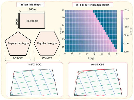
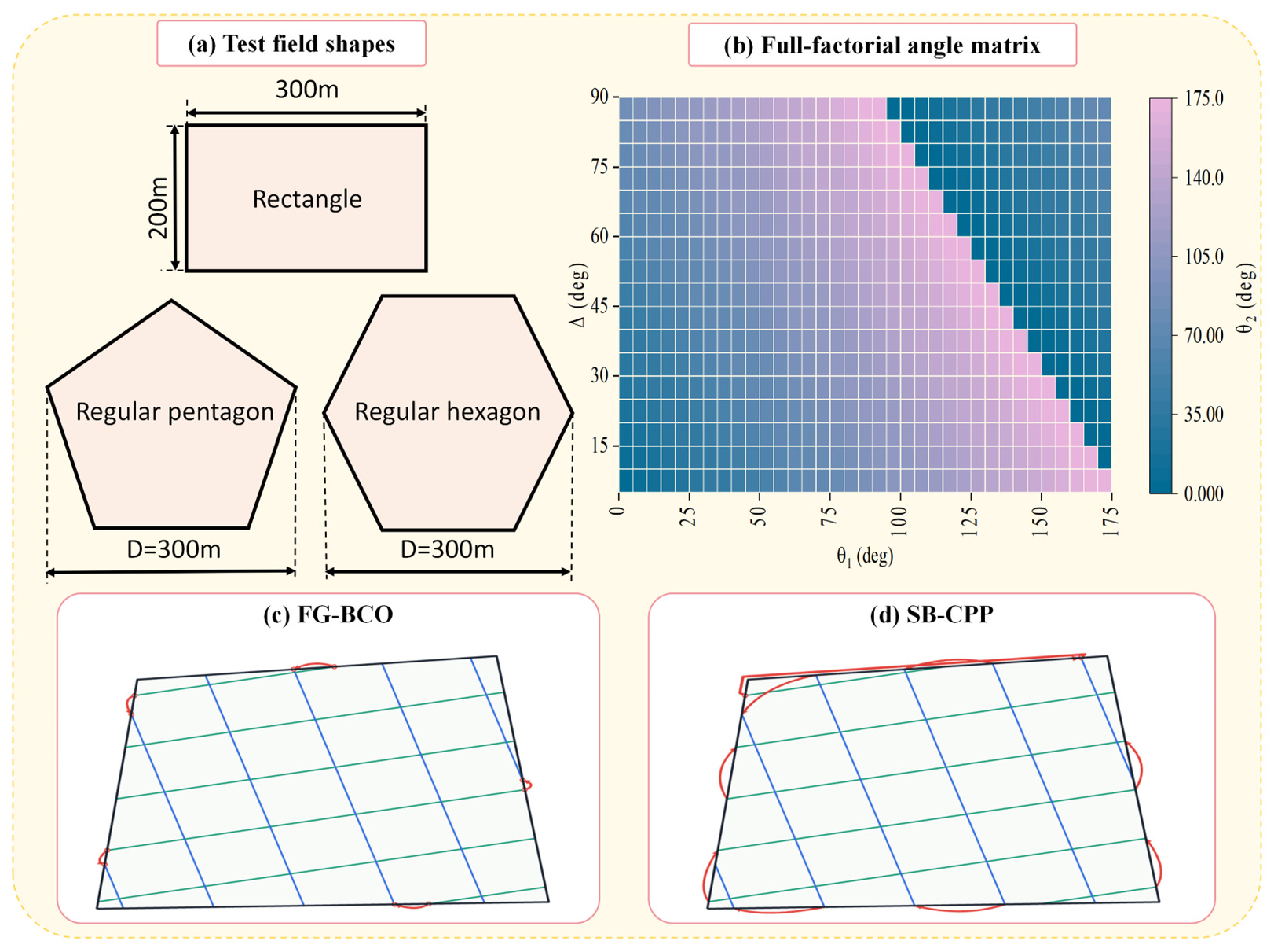
A full-factorial angle matrix was used to evaluate the effect of the two working directions. The first direction θ1 ranged from 0°to 175°at 5°intervals, giving 36 values. The included angle Δ ranged from 5°to 90°at 5° intervals, giving 18 values. The second direction θ2 was calculated using Equation (1). Restricting Δ to 90° or less removed equivalent supplementary direction pairs. Therefore, each field contained 648 distinct angle pairs. The complete angle matrix is shown in Figure 3b.
Figure 3.
Experimental design used for the paired simulations: (a) rectangular, regular pentagonal, and regular hexagonal test fields, D represents the characteristic size of the field; (b) full-factorial matrix of the first working orientation θ1 and included angle Δ, with color indicating the second working orientation θ2; (c) schematic route organization of FG-BCO; and (d) schematic route organization of SB-CPP.
All-path coverage was verified using a grid-based swept-area test. The field was discretized into square cells at a resolution of 0.25 m. For each cell center located inside the field polygon, the minimum distance to all executed path segments, including working, connection, and turning segments, was calculated. Because the implement width was 10 m and the implement was assumed to remain engaged along the complete route, a cell was classified as covered when this distance did not exceed 5 m. The all-path coverage rate was calculated as the number of covered in-field cells divided by the total number of in-field cells. The resulting value is therefore a numerical area estimate at the stated grid resolution rather than an exact analytical measure. This metric describes the nominal swept area obtained when the implement remains engaged along the entire route. It is a geometric estimate rather than an assessment of coverage uniformity, overlap, or agronomic coverage quality. In Figure 3c and Figure 3d, green and blue lines represent working segments from the first and second swath families, respectively; red lines represent connection and turning segments, and the dark outline indicates the field boundary.
Each field contained 648 matched angle pairs, giving 648 paired comparisons and 1296 algorithm–angle configurations across the two methods. The three regular fields contributed 1944 paired comparisons, and the irregular field contributed a further 648. Across all four fields, the evaluation comprised 2592 paired comparisons and 5184 algorithm–angle configurations. Repeated measurements for computational performance are described in Section 3.5.
3. Results and Discussion
3.1. Performance in Regular Fields
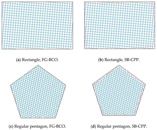
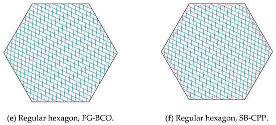
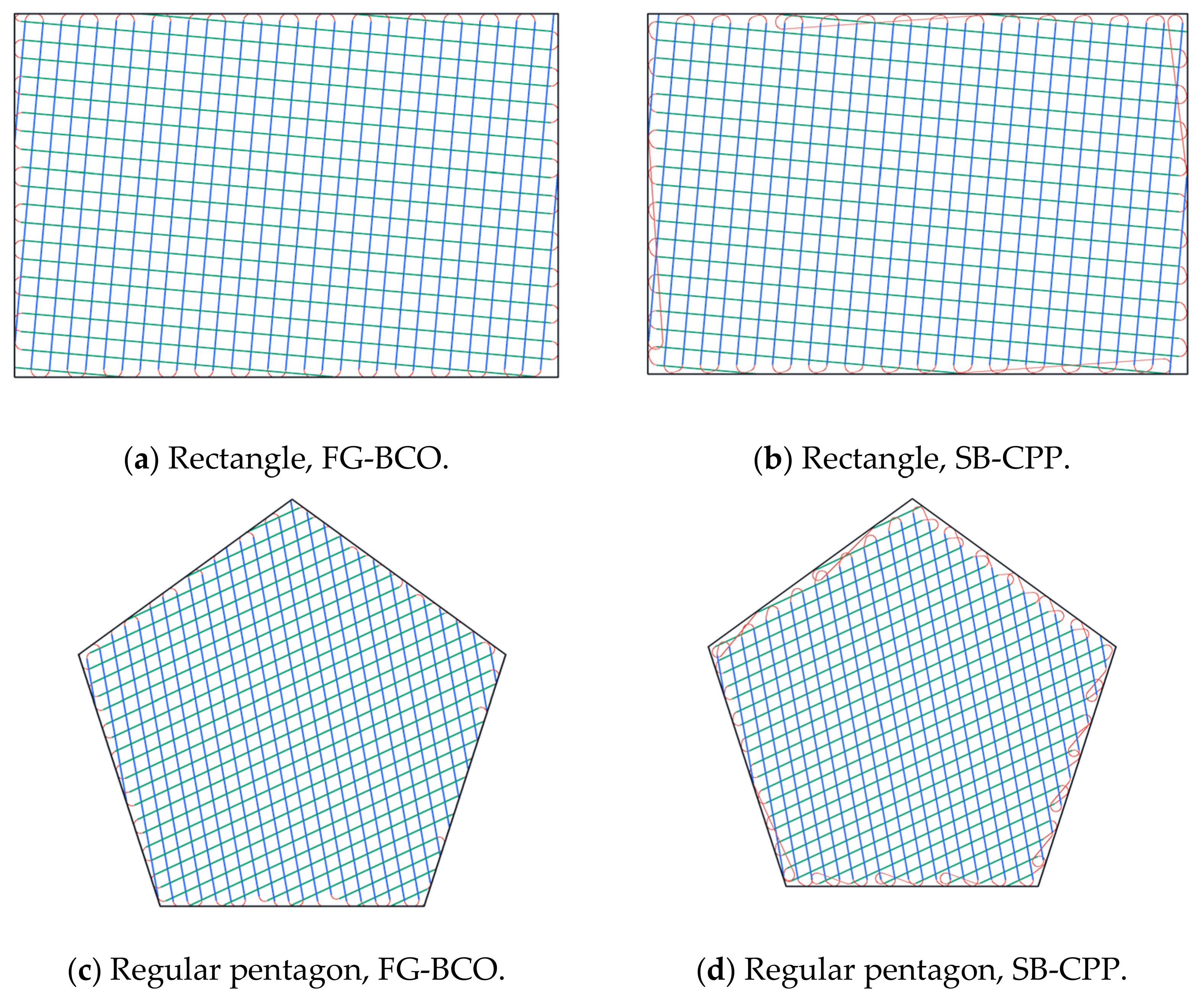
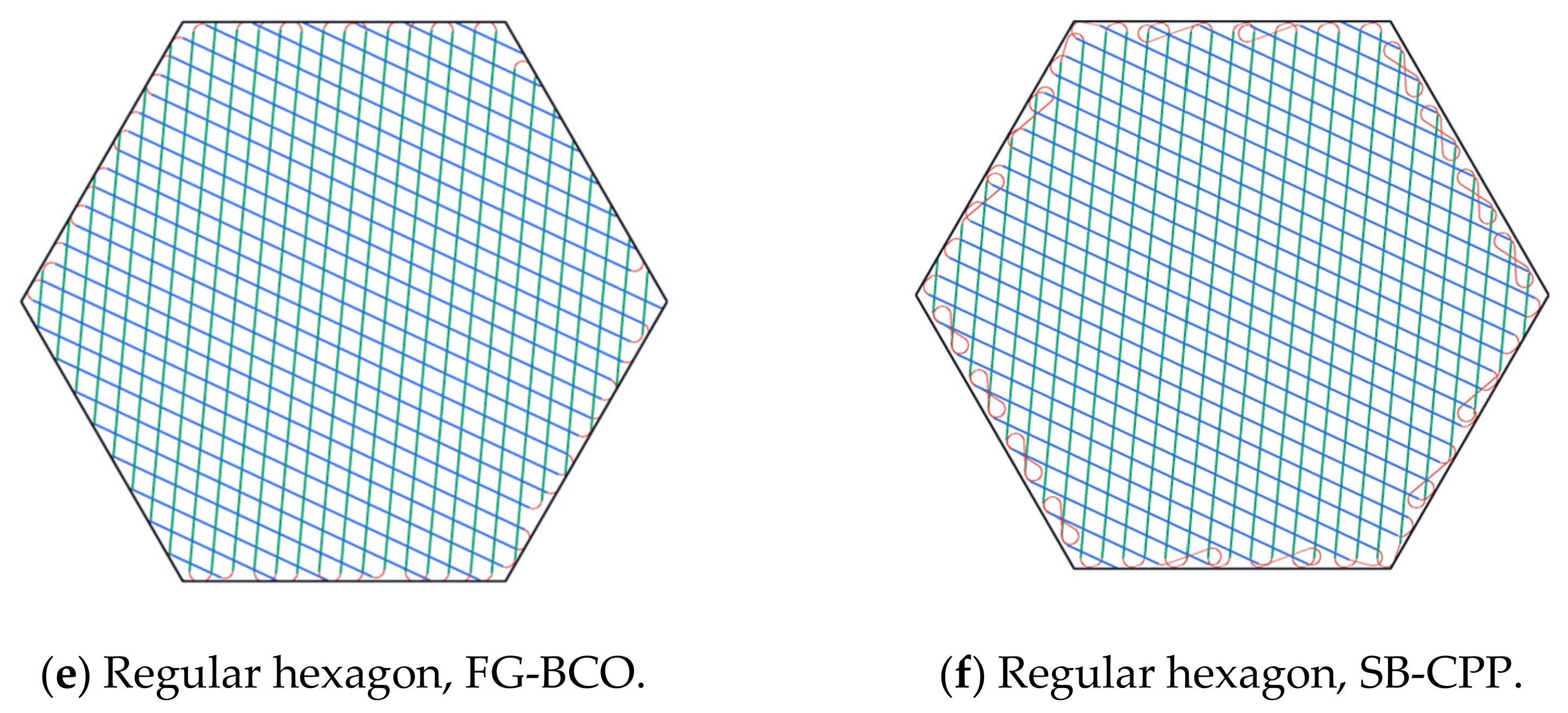
Figure 4 presents representative trajectories generated by FG-BCO and SB-CPP for the rectangular, regular pentagonal, and regular hexagonal fields. Within each paired comparison, the two methods use the same field boundary and prescribed coverage directions. Green and blue indicate working segments associated with the two directions, while red indicates connection and turning segments. These examples illustrate how the two planning strategies organize working segments and connect them near the field boundary.
Figure 4.
Representative high-coverage trajectories generated under matched angle pairs: (a,b) rectangular field; (c,d) regular pentagonal field; and (e,f) regular hexagonal field. Panels (a,c,e) show FG-BCO, while panels (b,d,f) show SB-CPP. Green and blue denote first- and second-direction working segments, red denotes connection and turning segments, and the dark outline denotes the field boundary. All displayed trajectories achieved an all-path coverage rate of 100%.
The reported comparison concerns the route beginning at the first working segment; the travel from the external reference point to this segment is not included. The results should therefore be interpreted as a comparison of the sequencing and connection strategy under a common coverage geometry, rather than as a complete operational route from the field entrance.
SB-CPP completes the working segments of the first pass before proceeding to the second, following a sequential back-and-forth pattern. In contrast, FG-BCO permits cross-pass interleaving and optimizes the visiting order and traversal orientation of the assembled route paths. Consequently, the two methods produce different connection patterns despite sharing the same prescribed coverage directions. The examples provide a qualitative illustration of these differences across field geometries. Their implications for total route length are evaluated over the complete angle-pair matrix in the following subsections.
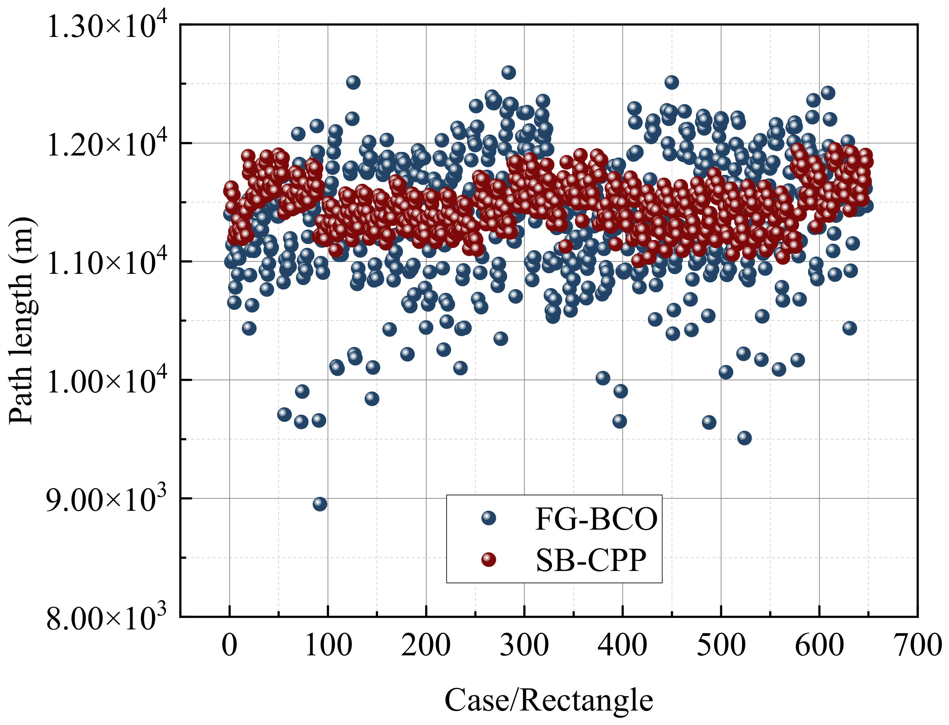
Figure 5 compares the total path lengths obtained for the rectangular field over all 648 angle pairs. The SB-CPP results remained concentrated at approximately 11,000–12,000 m, whereas FG-BCO exhibited a substantially wider response to the prescribed orientations. The broader FG-BCO distribution included both unfavorable angle pairs and a distinct lower tail, indicating that its connection strategy was more sensitive to the geometric relationship between the two swath families and the field boundary.
Figure 5.
Case-wise comparison of total path length obtained by FG-BCO and SB-CPP for the 648 angle pairs in the rectangular field.
The largest observed reduction in the rectangular field occurred in case 92, for which θ1 = 25° and Δ = 10°. FG-BCO generated a total path length of 8951.30 m, compared with 11,222.87 m for SB-CPP under the same angle pair, corresponding to a reduction of 20.24%. This case demonstrates the extent to which the combined ordering of the two swath families and the optimization of their connections can reduce travel when the selected orientations are favorable. At the same time, the scatter in Figure 5 shows that the improvement was not uniform across the entire angle matrix.
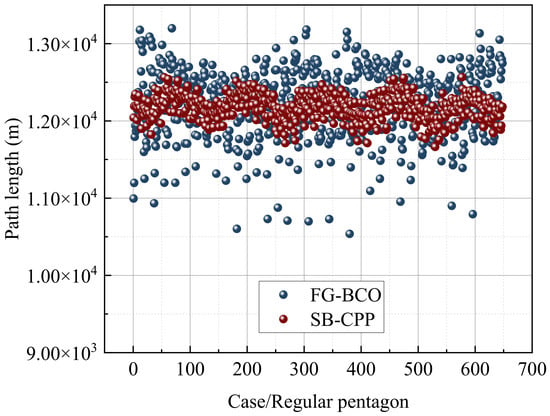
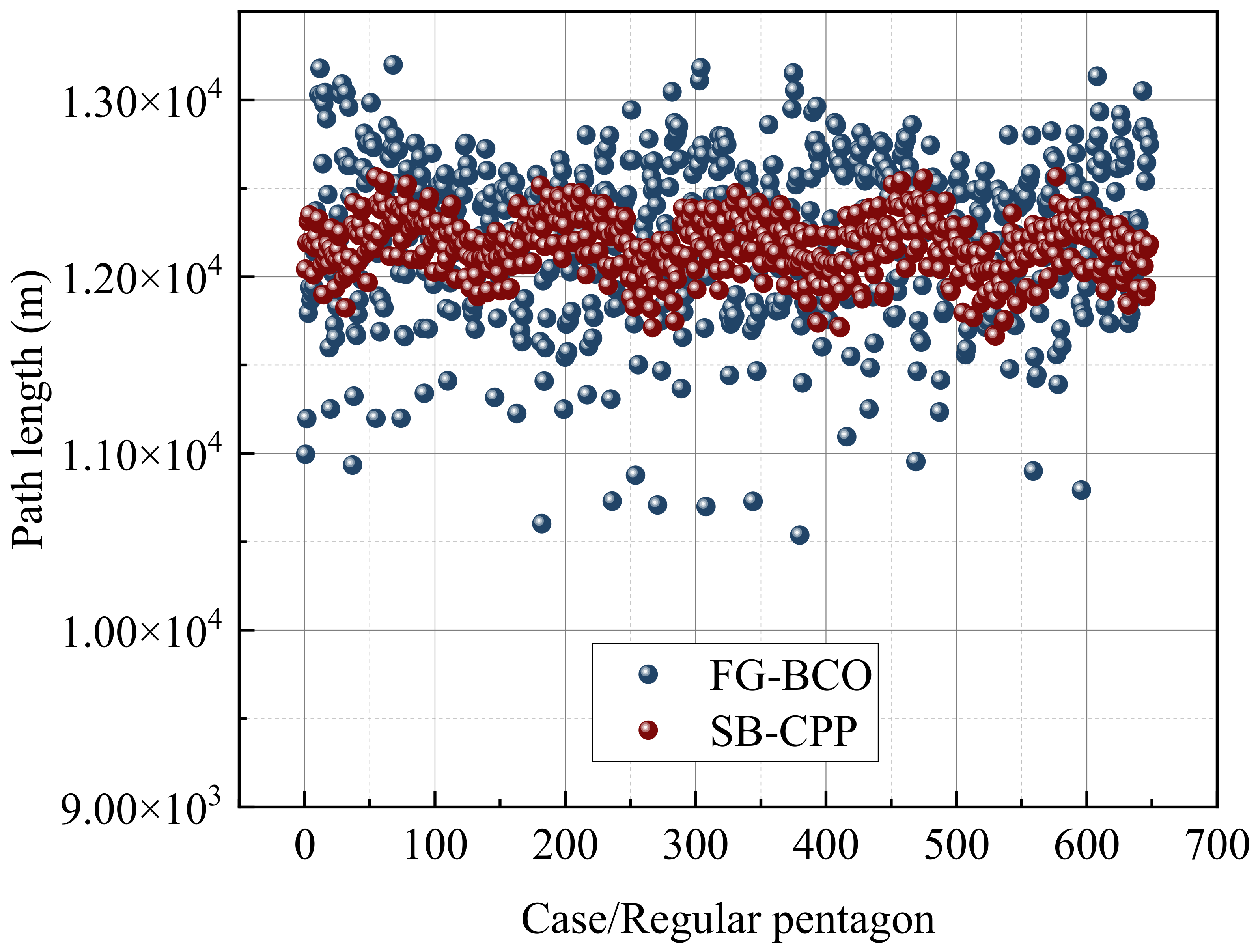
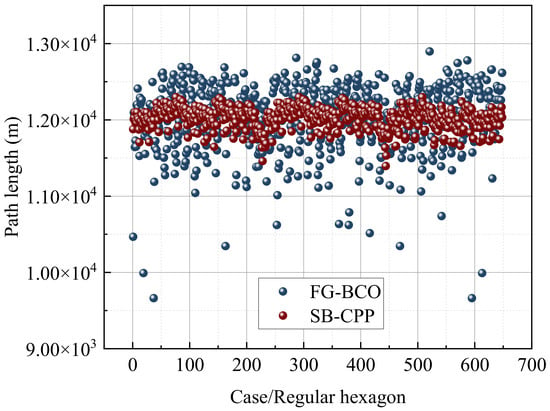
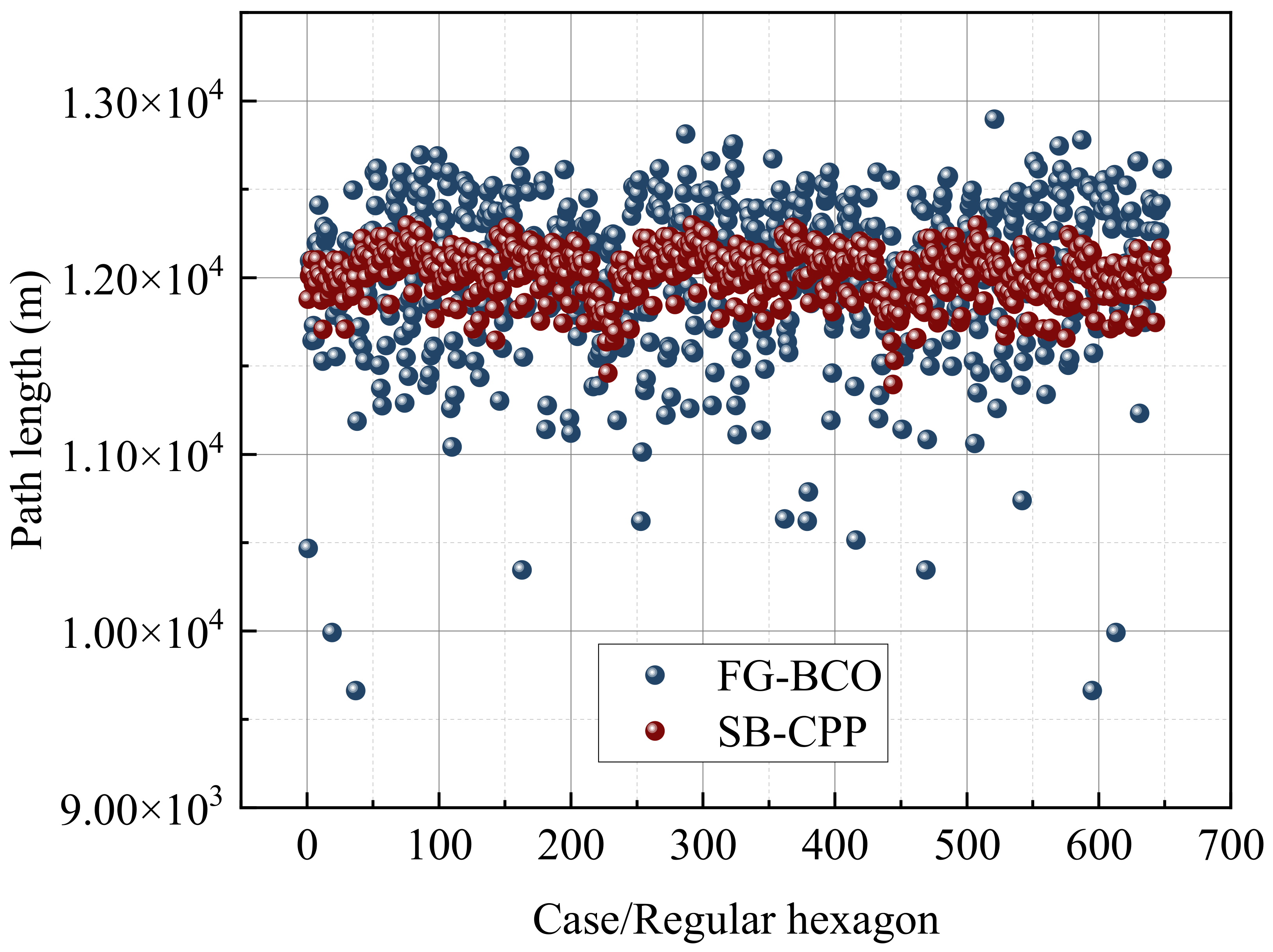
The same case-wise comparison was conducted for the regular pentagonal and hexagonal fields (Figure 6 and Figure 7). In both geometries, SB-CPP again formed a relatively compact band, while FG-BCO covered a wider range and produced lower minimum path lengths. The minimum FG-BCO path length was 10,537.70 m in the pentagonal field and 9662.84 m in the hexagonal field; the corresponding best SB-CPP values were 11,663.63 m and 11,395.18 m, respectively. Thus, the lower bound achieved by FG-BCO was reduced in all three field geometries, although the magnitude and frequency of the reductions varied with field shape.
Figure 6.
Case-wise comparison of total path length obtained by FG-BCO and SB-CPP for the 648 angle pairs in the regular pentagonal field.
Figure 7.
Case-wise comparison of total path length obtained by FG-BCO and SB-CPP for the 648 angle pairs in the regular hexagonal field.
A more pronounced lower tail was observed for the hexagonal field than for the pentagonal field. Several hexagonal cases approached or fell below 10,000 m, whereas the lowest pentagonal cases remained above 10,500 m. These differences show that field geometry affected not only the absolute route length but also the set of angle pairs from which FG-BCO could obtain short connections. The results therefore support evaluating the coverage directions jointly with the connection sequence rather than selecting an angle independently of the field boundary.
3.2. Performance in Irregular Fields
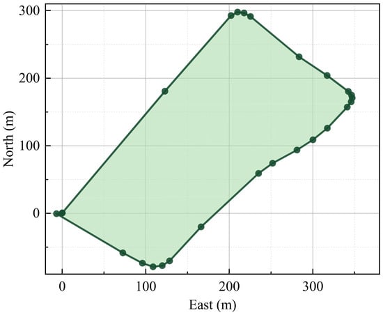
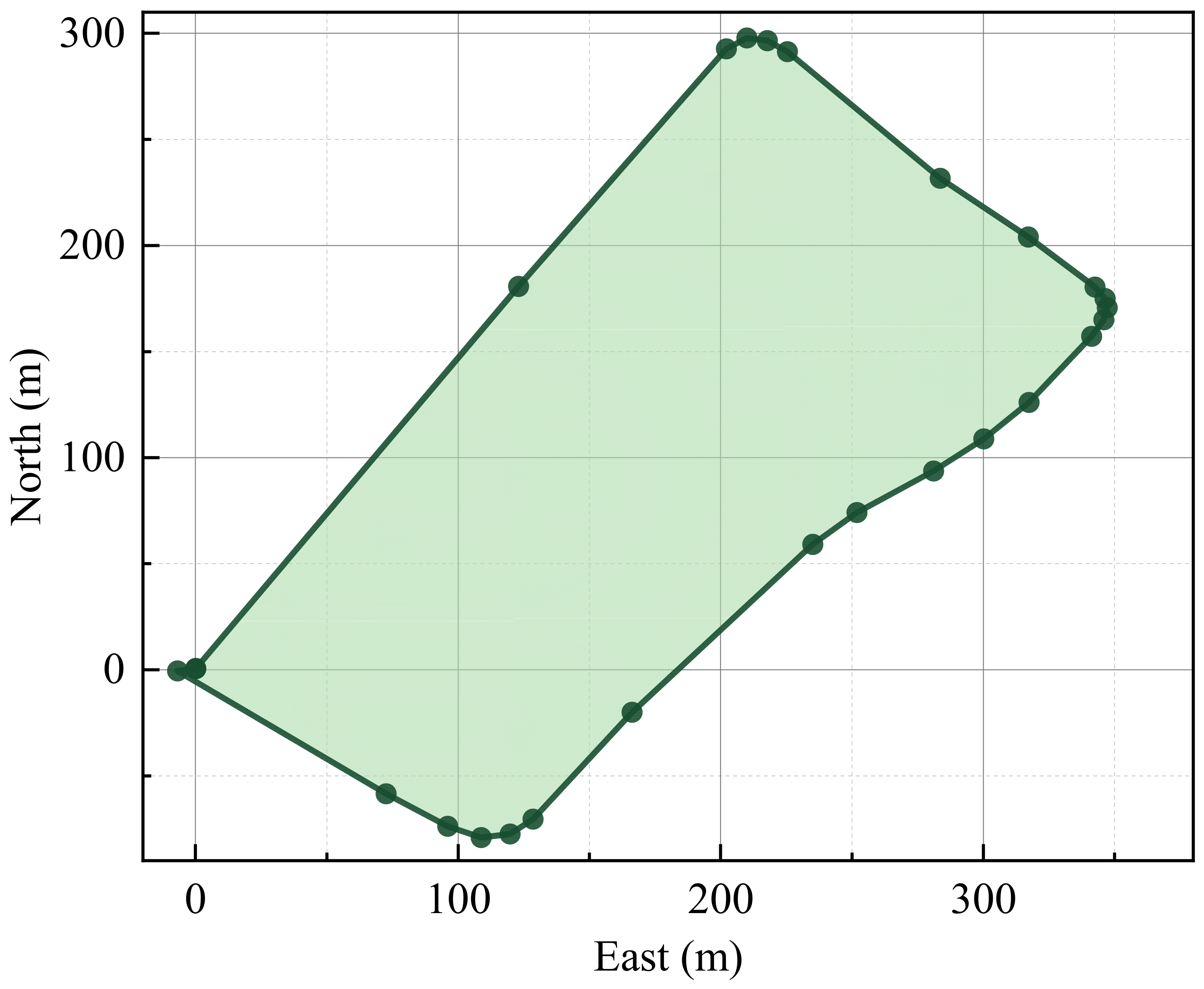
To extend the evaluation beyond idealized regular geometries, an additional case study was conducted using a field boundary derived from measured data. The boundary was sampled at approximately 0.1 m intervals, simplified to 25 vertices, and uniformly scaled to an area of 60,000 m2. Figure 8 shows the resulting field boundary and the start reference point. The field has an elongated outline with unequal boundary segments and locally varying boundary directions, providing an additional test of the relationship between field geometry and cross-pass connection planning.
Figure 8.
Irregular test field derived from measured boundary data, represented by 25 vertices and uniformly scaled to an area of 60,000 m2. Dark markers indicate boundary vertices.
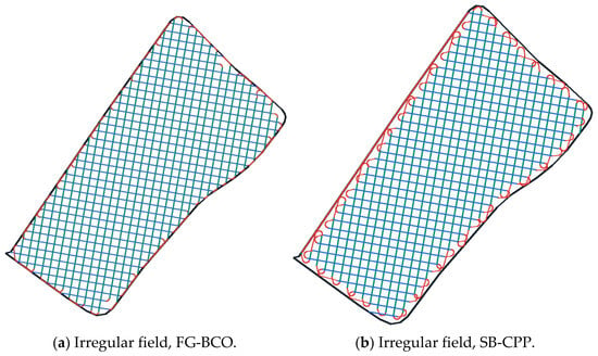
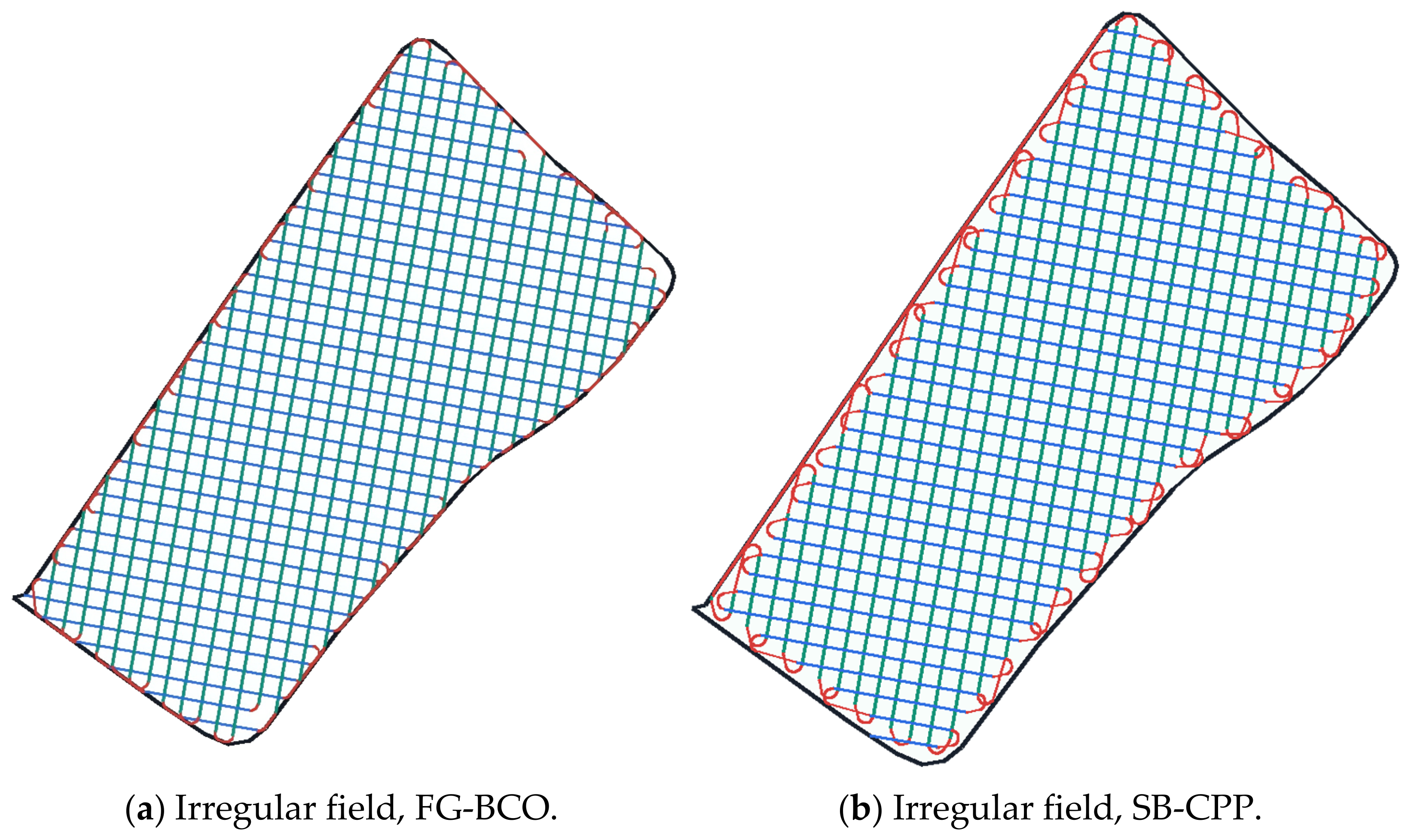
Figure 9 presents representative trajectories generated by FG-BCO and SB-CPP for the irregular field under the same prescribed coverage directions. Both methods adapt the working segments to the field boundary, while their different sequencing strategies lead to different connection patterns. SB-CPP retains the sequential back-and-forth organization within each pass, whereas FG-BCO permits connections between working segments from different passes. These differences are visible near the field boundary, where the two methods connect the same swath families in different ways.
Figure 9.
Representative trajectories generated under a matched angle pair in the irregular field: (a) FG-BCO; (b) SB-CPP. Green and blue denote first- and second-direction working segments, red denotes connection and turning segments, and the dark outline denotes the field boundary.
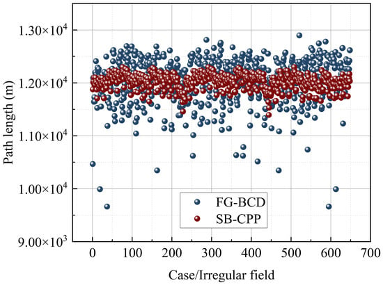
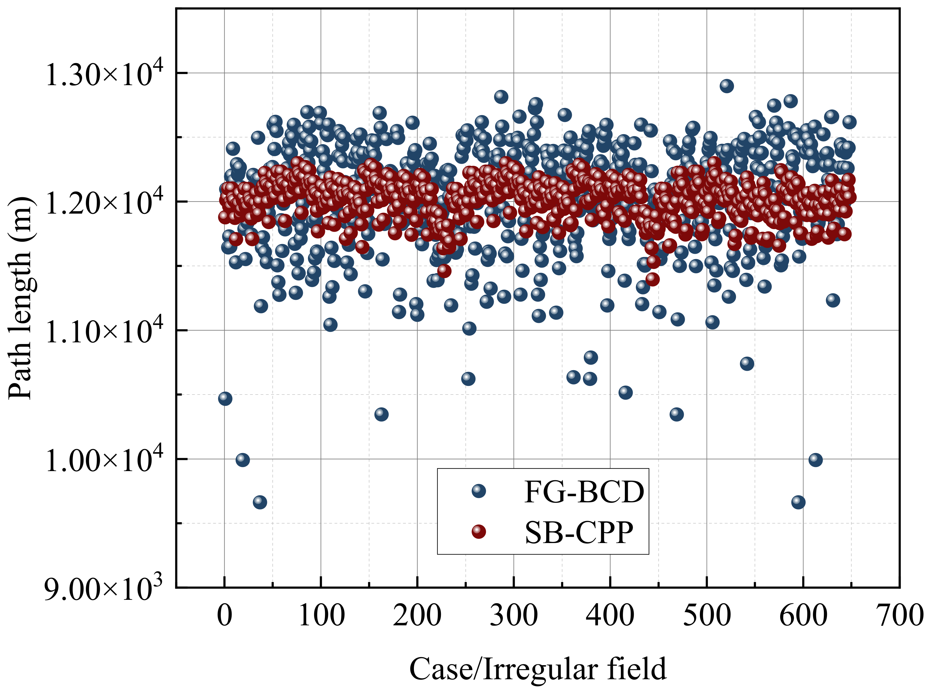
The comparison was extended to an irregular field using 648 matched angle pairs (Figure 10). FG-BCO produced a minimum path length of 9717.23 m, compared with 11,722.37 m for SB-CPP, corresponding to a 17.11% reduction between the independently selected grid minima. The largest matched-case saving was 23.55% in case 91, where the FG-BCO and SB-CPP path lengths were 9717.23 and 12,710.06 m, respectively. However, FG-BCO generated shorter routes in only 263 cases (40.59%). Its mean path length was 12,453.24 m, compared with 12,357.24 m for SB-CPP. Thus, the irregular field also exhibited favorable individual cases and a lower grid minimum, but these advantages did not translate into a shorter average route across all prescribed angle pairs.
Figure 10.
Case-wise comparison of total path length obtained by FG-BCO and SB-CPP for the 648 angle pairs in the irregular field.
3.3. Distribution of Total Path Length
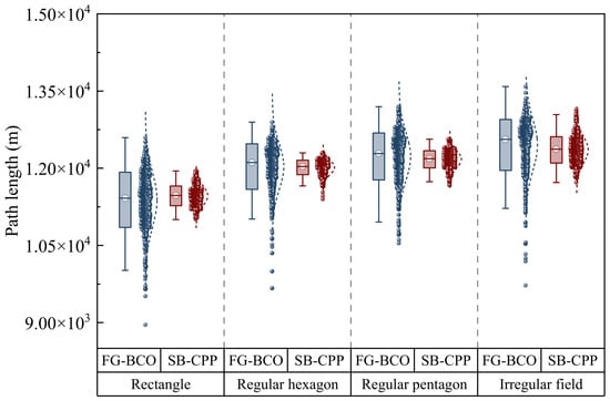
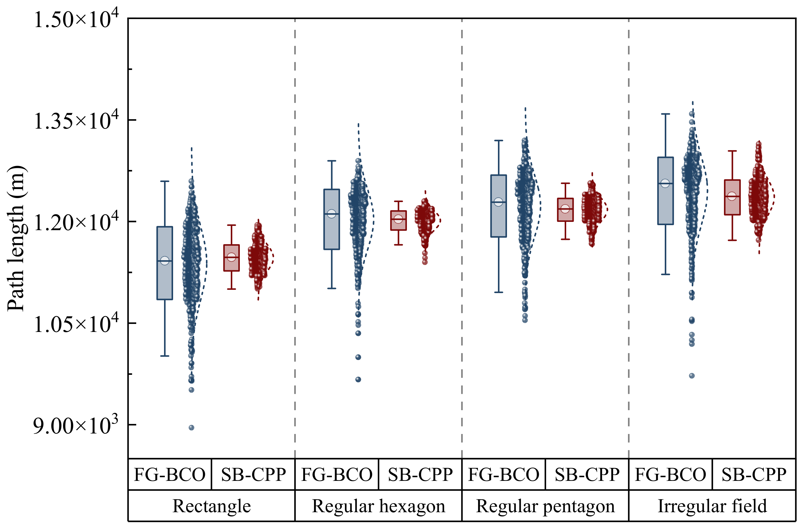
Figure 11 summarizes the total path-length distributions for the rectangular, regular hexagonal, regular pentagonal, and irregular fields. FG-BCO exhibited greater dispersion than SB-CPP and attained a lower minimum path length in each field. Its minimum lengths were 8951.30, 9662.84, 10,537.70, and 9717.23 m, respectively. The corresponding SB-CPP minima were 11,003.84, 11,395.18, 11,663.63, and 11,722.37 m. The relative reductions between these independently selected minima were 18.65%, 15.20%, 9.65%, and 17.11%. These values describe the best observed results within the tested angle grid rather than typical performance under prescribed angles.
Figure 11.
Box plots and individual observations of total path length for FG-BCO and SB-CPP in the four fields.
The lower FG-BCO minima did not imply lower average path lengths in every field. In the irregular field, for example, the mean FG-BCO path was 96.01 m longer than the mean SB-CPP path. The broad FG-BCO distributions therefore reflect both opportunities for substantial reductions and sensitivity to the selected angle pair. Since the separate box plots do not preserve the correspondence between the methods at each angle pair, the paired saving distributions are examined in Section 3.4 to quantify improvements and degradations directly.
3.4. Path-Length Saving Rate and Asymmetric Performance
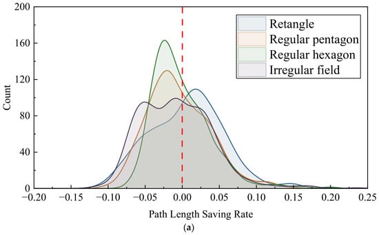
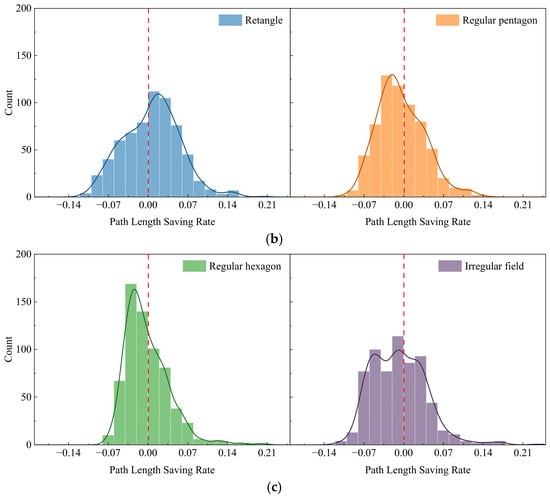
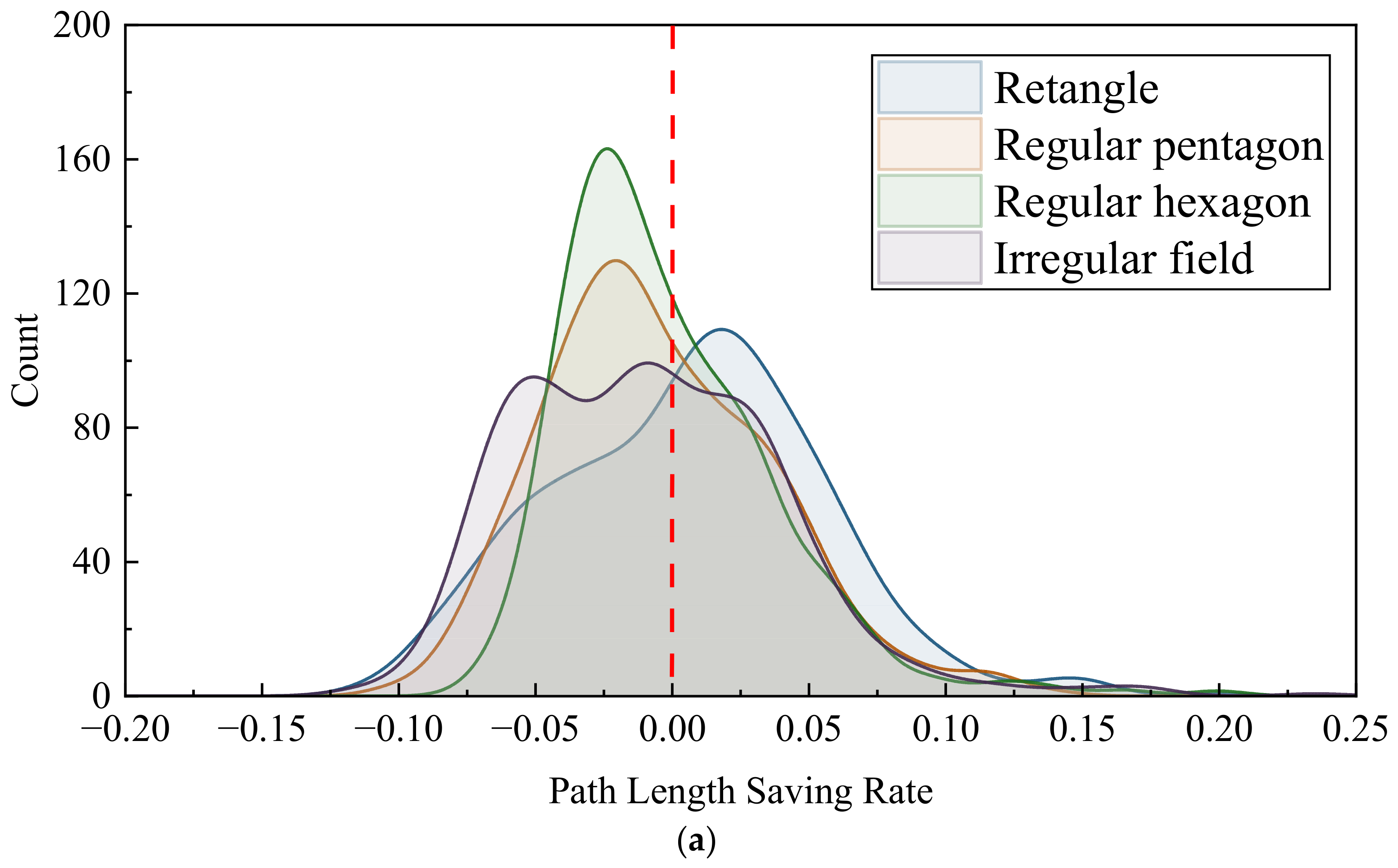
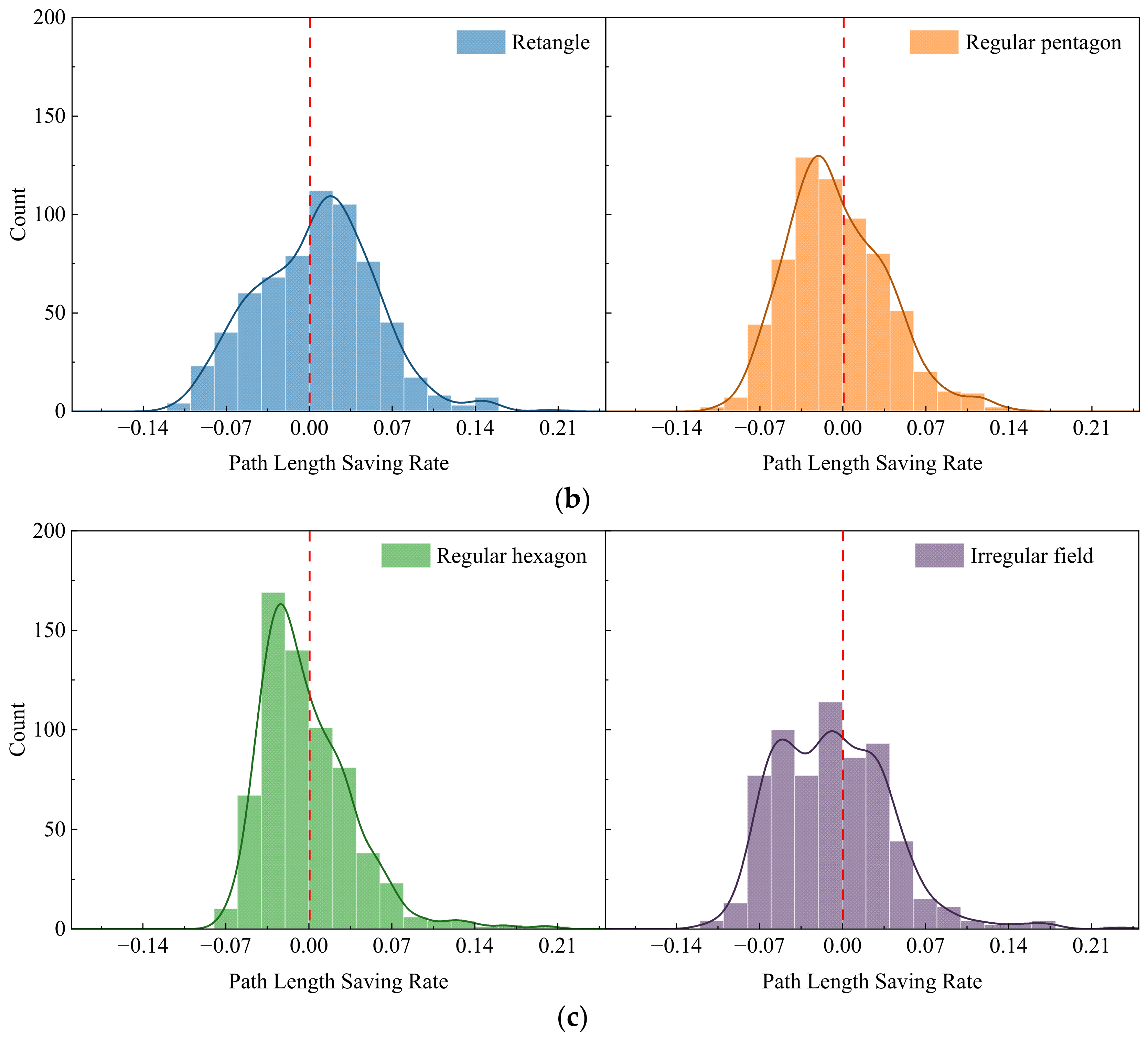
To compare the two methods on a relative basis, the path-length saving rate was calculated as (SB-CPP − FG-BCO)/SB-CPP, so that a positive value indicates a shorter FG-BCO route. Positive values indicate shorter FG-BCO routes, whereas negative values indicate longer routes. Figure 12 presents the distributions across 648 matched angle pairs for each field. FG-BCO generated shorter routes in 375 rectangular cases (57.87%), 271 pentagonal cases (41.82%), 262 hexagonal cases (40.43%), and 263 irregular-field cases (40.59%). Thus, improvements occurred in a majority of the rectangular cases, while degradations were more frequent in the other three fields. The mean saving rates were 0.646%, −0.484%, −0.144%, and −0.833% for the rectangular, regular pentagonal, regular hexagonal, and irregular fields, respectively. The corresponding medians were 0.939%, −1.060%, −0.923%, and −1.094%. The vertical red dashed lines indicate zero saving, corresponding to equal path lengths for the two algorithms. Positive values indicate shorter FG-BCO routes, whereas negative values indicate longer FG-BCO routes. These statistics are consistent with the dominant positive peak for the rectangle and the principal negative peaks for the other fields in Figure 12. The rectangle provided a modest positive average saving. In contrast, neither the mean nor the median indicated an overall advantage in the remaining fields. For the hexagon, the mean was closer to zero than the median, reflecting the influence of relatively large savings in a smaller subset of cases.
Figure 12.
Distribution of the path-length saving rate of FG-BCO relative to SB-CPP for the tested field geometries: (a) overlaid kernel density estimates; (b) histograms and fitted density curves for the rectangular and regular pentagonal fields; and (c) histograms and fitted density curves for the regular hexagonal and irregular fields.
The positive tails contained substantial individual improvements. Maximum savings reached 20.24%, 14.24%, 20.38%, and 23.55% in the rectangular, pentagonal, hexagonal, and irregular fields, respectively. However, the largest path-length increases were also considerable, reaching 11.17%, 10.39%, 7.64%, and 11.64%. The irregular field therefore produced both the largest observed saving and the largest degradation among the four benchmarks. Moreover, savings exceeding 5% occurred in only 9.41% of its cases, whereas path-length increases exceeding 5% occurred in 22.38%. Its extended positive tail consequently did not indicate a favorable overall distribution.
The irregular-field results further illustrate the balance between improvement frequency and magnitude. The 263 improved cases achieved an average saving of 3.779%, while the 385 degraded cases incurred an average increase of 3.984%. Their frequency-weighted contributions were +1.534 and −2.367 percentage points, yielding the net mean saving of −0.833%. Degradations were therefore both more frequent and slightly larger on average. These results distinguish substantial savings under favorable angle combinations from performance across the full prescribed-angle grid. FG-BCO offers opportunities for shorter routes, but realizing those opportunities requires angle-pair evaluation and cannot be assumed for an arbitrary prescribed orientation.
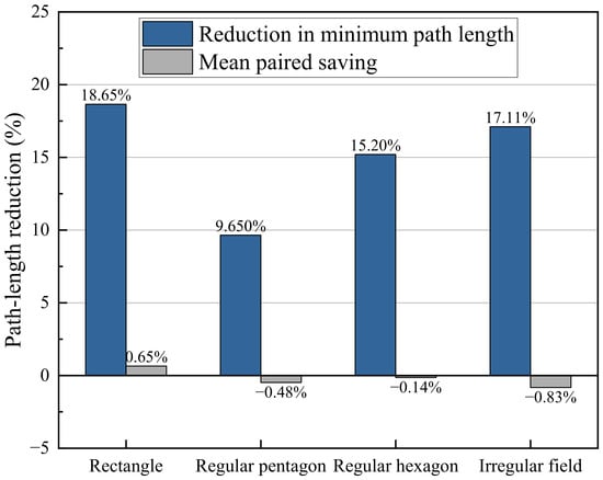
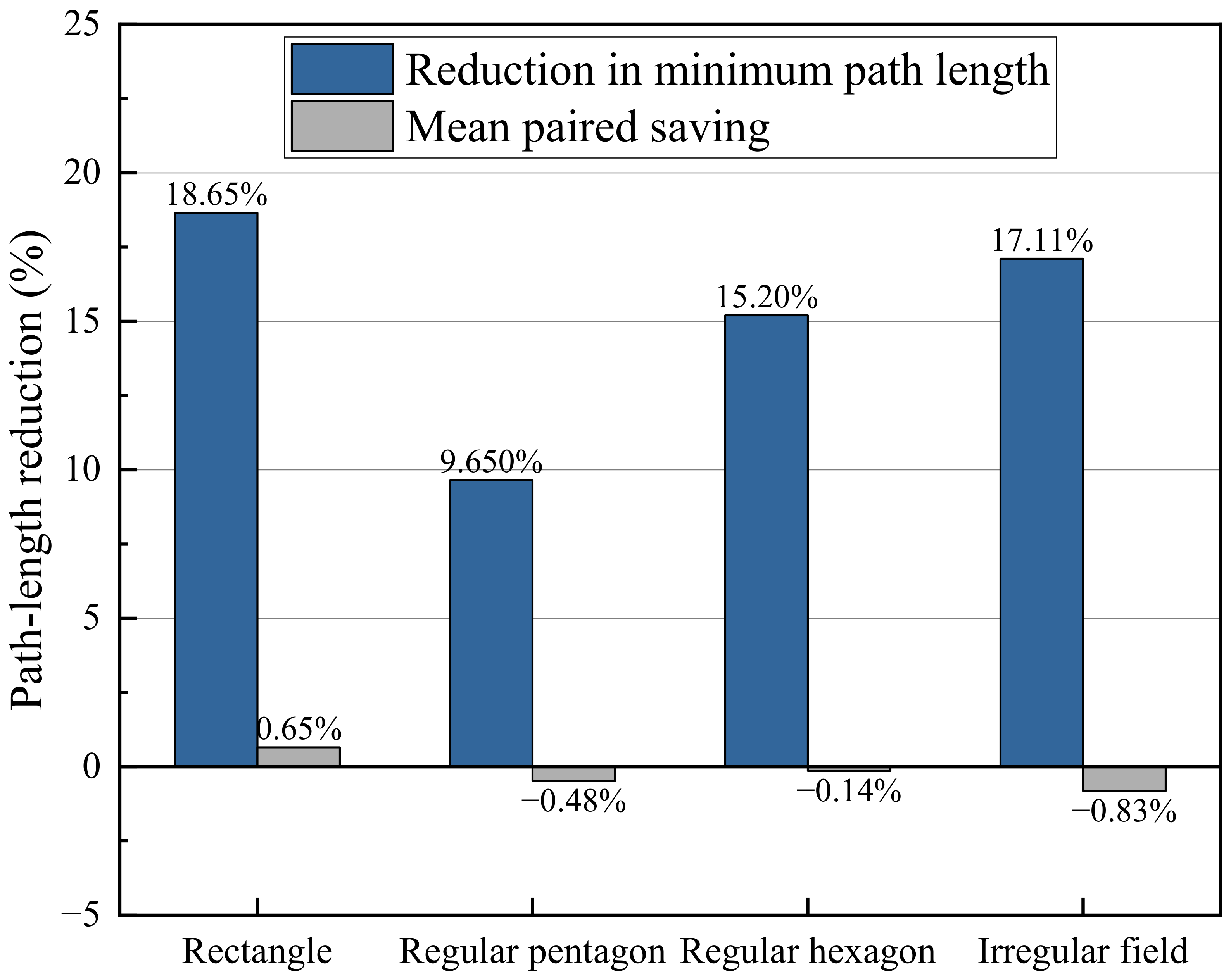
Figure 13 compares the relative reductions in minimum path length with the mean paired savings across all tested angle combinations. The minimum path length of each algorithm was determined independently from the 648 angle pairs. FG-BCO achieved shorter minimum paths than SB-CPP in all four fields, with reductions of 18.65%, 9.65%, 15.20%, and 17.11% for the rectangular, regular pentagonal, regular hexagonal, and irregular fields, respectively. The largest reduction occurred in the rectangular field, followed by the irregular and hexagonal fields. However, the corresponding mean paired savings were only 0.646%, −0.484%, −0.144%, and −0.833%. This difference shows that the advantage in minimum path length does not imply an average improvement across prescribed angle pairs. FG-BCO can produce substantially shorter routes when suitable coverage directions are selected, but its benefit remains dependent on the combination of field geometry and coverage orientation.
Figure 13.
Comparison of minimum path-length reductions and mean paired savings of FG-BCO relative to SB-CPP across four field geometries.
The non-uniform performance can be interpreted from the interaction between swath geometry and route construction. Both methods start from the same line–polygon intersections, but organize the resulting working segments differently. Cross-pass connections in FG-BCO are favorable when endpoints from the two swath families are close along the boundary, their traversal headings are compatible, and sufficient turning space is available. Conversely, dispersed endpoints, unfavorable heading changes, and short segments with limited turning space can restrict feasible links and increase the connections required between assembled route paths. Swath number and length distribution therefore influence performance through endpoint placement and connection feasibility rather than through a simple monotonic relationship with route length.
The relative pass angle affects heading compatibility, whereas the absolute orientations relative to the field edges determine the clipped swaths and their endpoint configuration. Consequently, the relative angle alone cannot identify advantageous cases. Field symmetry may create repeated favorable configurations, but does not ensure a benefit across orientations, as illustrated by the 40.43% improvement frequency in the regular hexagon. Furthermore, FG-BCO constructs route paths using local connection rules before optimizing their order and traversal orientations. This optimization is conditional on the assembled paths and does not guarantee a shorter final route than SB-CPP for every angle pair. These mechanisms provide a qualitative interpretation of the observed variability; the present analysis does not establish universal favorable angle ranges or quantify the independent contribution of each geometric factor. Preliminary evaluation should therefore consider both working directions together with the target field boundary.
3.5. Additional Performance Evaluation
Computational runtime and memory usage were evaluated to complement the path-length comparisons presented above.All experiments were conducted on a computer equipped with an Intel Core i5-14600K processor (Intel Corporation, Santa Clara, CA, USA) and 32 GB of RAM, running 64-bit Windows 11 Pro (version 25H2). Both FG-BCO and SB-CPP were implemented in Python (version 3.14.2). FG-BCO and SB-CPP were compared in the rectangular, regular pentagonal, regular hexagonal, and irregular fields. Runtime measurements excluded the final geometric validation, and memory usage represented the total memory used by the process. Warm-up runs were performed before repeated measurements, and the measurements for each algorithm–angle configuration were averaged. For each algorithm and field, the medians of these per-configuration averages over the 648 tested angle pairs are reported. These metrics describe computational resource usage rather than the time required to execute the resulting tractor routes.
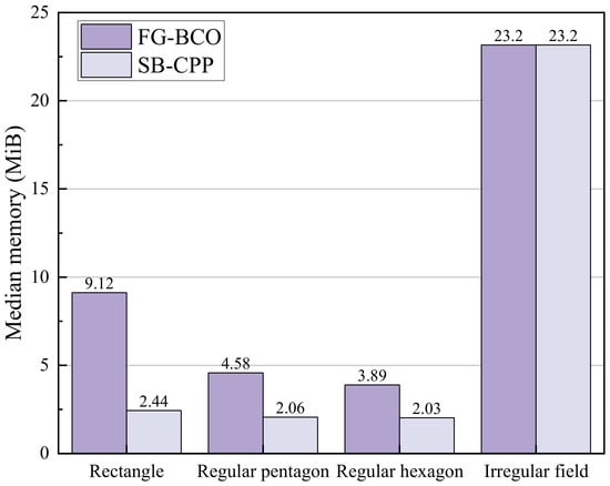
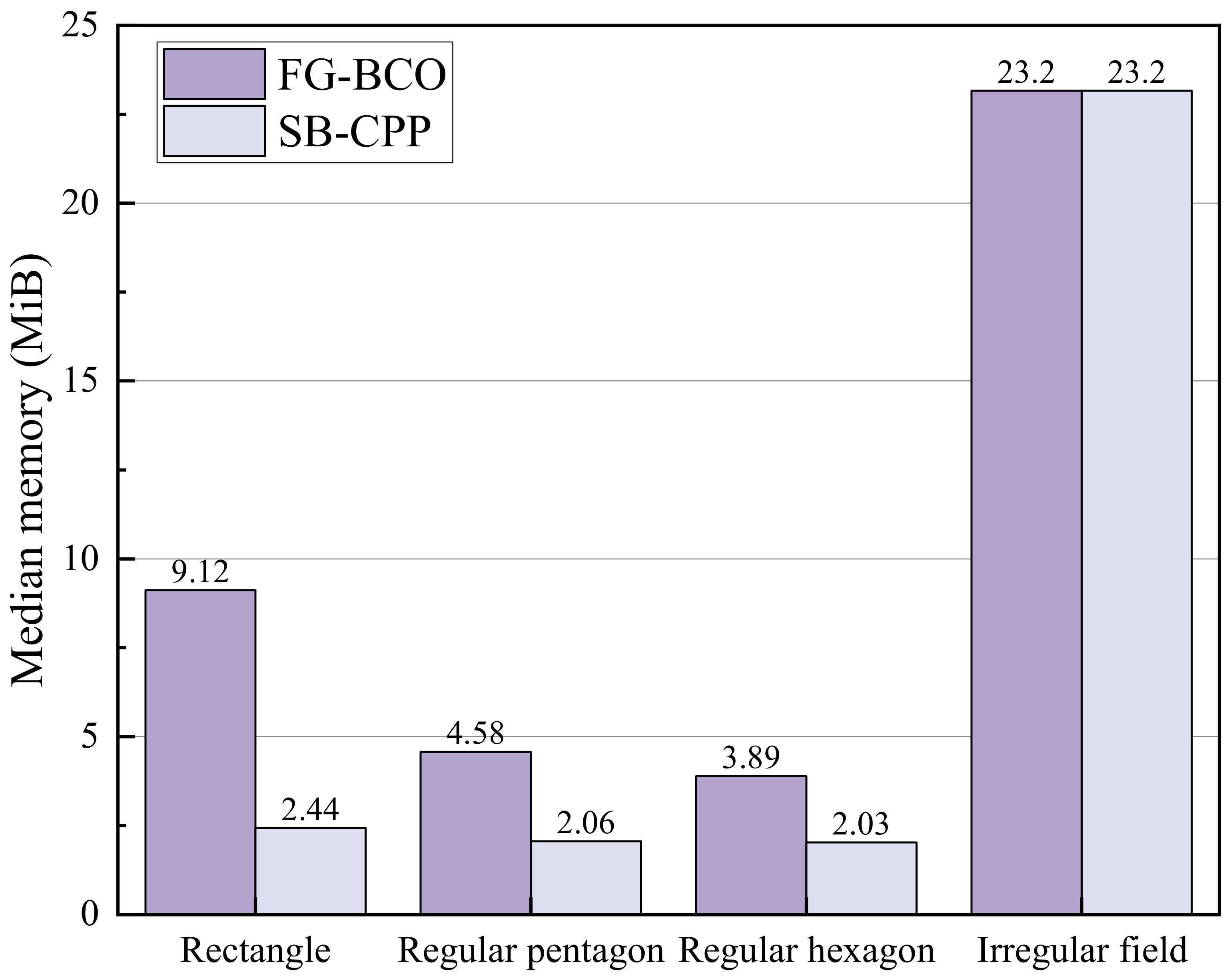
Figure 14 compares the median runtimes of the two methods. FG-BCO required 9.12, 4.58, and 3.89 ms in the rectangular, regular pentagonal, and regular hexagonal fields, respectively, compared with 2.44, 2.06, and 2.03 ms for SB-CPP. Although the relative differences were appreciable, the absolute increases were limited to 1.86–6.68 ms. In the irregular field, both methods had a median runtime of approximately 23.2 ms at the reported precision. Thus, FG-BCO incurred additional computational cost in the regular fields, while the median runtimes remained below 24 ms for both methods across all four tested geometries.
Figure 14.
Median runtime of FG-BCO and SB-CPP across the four test fields. Each value is the median of the mean runtimes obtained from repeated measurements after warm-up for the 648 angle pairs.
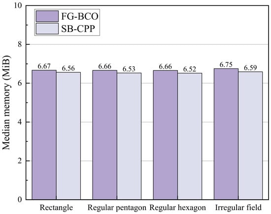
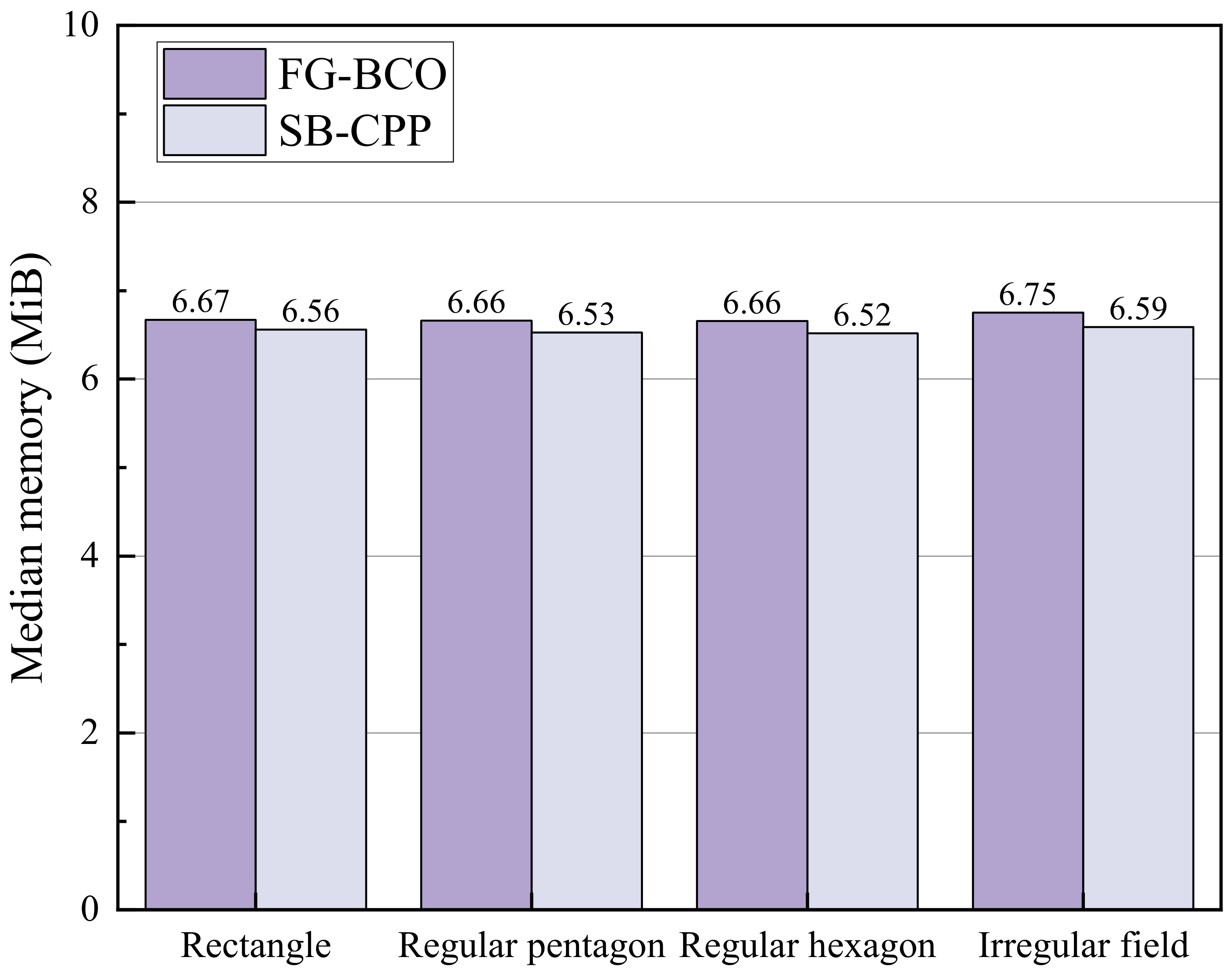
Figure 15 shows that memory usage was closely comparable between the two algorithms. The median values for FG-BCO ranged from 6.66 to 6.75 MiB, whereas those for SB-CPP ranged from 6.52 to 6.59 MiB. FG-BCO used slightly more memory in every field, with differences of only 0.11–0.16 MiB. Memory usage also varied little across the four geometries for either method.
Figure 15.
Median total process memory usage of FG-BCO and SB-CPP across the four test fields. Each value is the median of the mean memory measurements obtained from repeated measurements after warm-up for the 648 angle pairs.
These results indicate that the path-reduction opportunities provided by FG-BCO were accompanied by a small absolute runtime overhead in the regular fields and a limited increase in memory usage across all tested fields. Within the evaluated configurations, the additional sequencing and connection optimization therefore remained modest in its computational resource requirements.
4. Conclusions
This study developed FG-BCO for autonomous two-pass diagonal harrowing in polygonal fields. The method clips two swath families to the field boundary, assembles cross-pass working segments into alternating route paths, and jointly optimizes the order and traversal orientation of these route paths. Boundary-aware transfers and curvature-constrained smoothing are subsequently applied to obtain forward-only trajectories satisfying the prescribed minimum turning radius and boundary-containment requirements for the vehicle reference point.
Across 648 matched angle pairs per field, FG-BCO achieved shorter routes than SB-CPP in 57.87%, 41.82%, 40.43%, and 40.59% of the cases for the rectangular, regular pentagonal, regular hexagonal, and irregular fields, respectively. The corresponding mean paired saving rates were 0.646%, −0.484%, −0.144%, and −0.833%, while the medians were 0.939%, −1.060%, −0.923%, and −1.094%. FG-BCO therefore provided a modest overall advantage in the rectangular field, whereas improvements were less frequent than degradations in the other three fields. When the minimum path length of each algorithm was selected independently over the tested angle pairs, FG-BCO reduced these best-achieved path lengths by 18.65%, 9.65%, 15.20%, and 17.11%, respectively. These reductions represent the potential benefit obtainable through suitable angle selection and should not be interpreted as the expected improvement for an arbitrary prescribed angle pair.
The non-uniform performance arises from the interaction between field geometry, working directions, and connection construction. FG-BCO is more likely to be advantageous when endpoints from the two swath families are close along the boundary, their traversal headings are compatible, and sufficient turning space is available. Endpoint mismatch, unfavorable heading changes, and short swaths with limited turning space can restrict feasible cross-pass links and increase travel between the assembled route paths. The relative pass angle affects heading compatibility, while the absolute orientations relative to the field boundary determine swath lengths and endpoint configurations. Consequently, FG-BCO should be applied together with a preliminary evaluation of feasible angle pairs for the target field.
The additional sequencing and connection optimization introduced only modest computational overhead. Across the four fields, the median runtime remained below 24 ms for both methods. FG-BCO required an additional 1.86–6.68 ms in the regular fields, while the two methods had approximately equal median runtimes in the irregular field at the reported precision. The median memory difference was limited to 0.11–0.16 MiB.
The present evaluation concerns geometric planning in obstacle-free planar fields and assesses feasibility at the vehicle-reference-point level. It does not establish clearance for the full tractor–implement footprint or account for terrain effects, wheel slip, speed-dependent dynamics, or tracking uncertainty. The all-path coverage metric describes the union of the swept areas and does not verify complete coverage in each working direction separately. In addition, the two methods retain different start-selection rules, and access and departure travel are excluded from the reported path lengths. These assumptions should be considered when interpreting the results and extending the method to field operation.
Future work will incorporate tractor–implement footprint constraints and site-specific boundary clearances, evaluate routes under a common physical starting condition, and validate execution through autonomous tractor experiments. Further evaluation will examine parameter sensitivity, working and connection distances, turning characteristics, and coverage by each swath family. Comparisons with additional optimization-based planners will require a common formulation of the two-pass planning task. Time and energy models will also be needed to determine how geometric path reductions translate into operational benefits.
Author Contributions
Conceptualization, J.W. and X.H.; Methodology, J.W. and X.H.; Validation, J.W. and X.H.; Formal Analysis, J.W.; Investigation, J.W.; Writing—Original Draft Preparation, J.W.; Writing—Review and Editing, Y.W. and X.Z.; Visualization, Y.W.; Writing—Review and Editing; Supervision; Project Administration, J.C. All authors have read and agreed to the published version of the manuscript.
Funding
This research received no external funding.
Institutional Review Board Statement
Not applicable.
Informed Consent Statement
Not applicable.
Data Availability Statement
The original contributions presented in this study are included in the article; further inquiries can be directed to the corresponding author.
Conflicts of Interest
Author Jin Wang was employed by the company Guangdong Sfoundint Technology Co., Ltd. The remaining authors declare that the research was conducted in the absence of any commercial or financial relationships that could be construed as a potential conflict of interest.
Abbreviations
| CCPP | Complete Coverage Path Planning |
| FG-BCO | Field-Geometry-Aware Bidirectional Coverage and Connection Path Co-Optimization |
| SB-CPP | Sequential Boustrophedon Coverage Path Planning |
| Ω | Polygonal field region |
| ∂Ω | Boundary of the polygonal field |
| θ1,θ2 | Working orientations of the first and second harrowing passes |
| Δ | Smaller included angle between the two working orientations |
| W | Implement working width and nominal spacing between adjacent swaths |
| Rmin | Prescribed minimum turning radius |
| k | Harrowing-pass index |
| μk | Unit vector along the working direction of pass k |
| nk | Unit normal vector of the working direction of pass k |
| ck,min,ck,max | Minimum and maximum projected coordinates of the field along nk |
| ck,m | Lateral offset of line m in pass k |
| m | Parallel-line index within a harrowing pass |
| Nk | Number of parallel working lines generated for pass k |
| Sk,m | Boundary-clipped working segment corresponding to line m in pass k |
| x | Point in the two-dimensional Cartesian coordinate system |
| ℝ2 | Two-dimensional Euclidean space |
| i,j | Indices of oriented working segments or route paths, as applicable |
| Exit endpoint of oriented segment or route path i | |
| Entry endpoint of oriented segment or route path j | |
| β | Weight assigned to the Euclidean-distance term in the local connection cost |
| gij | Local connection cost from oriented segment i to oriented segment j |
| pi | Route path i |
| Q | Number of route paths |
| a,b | Binary traversal-orientation states of two route paths |
| cij(a,b) | Transition cost from path i in orientation a to path j in orientation b |
| pint | Penalty for a transition involving a near-boundary intersection |
| phead | Penalty for an unfavorable departure or arrival heading |
| pturn | Penalty for insufficient turning space |
| λint | Weight assigned to the near-boundary intersection penalty |
| λhead | Weight assigned to the unfavorable-heading penalty |
| π | Route-path visiting-order vector |
| b | Route-path traversal-orientation vector |
| q | Position index in the route-path visiting sequence |
| J* | Minimum accumulated transition cost |
| N | Total number of retained working segments |
| V | Number of field-boundary edges |
| E | Number of feasible candidate links in the endpoint graph |
References
- Höffmann, M.; Patel, S.; Büskens, C. Optimal guidance track generation for precision agriculture: A review of coverage path planning techniques. J. Field Robot. 2024, 41, 823–844. [Google Scholar] [CrossRef] [Scilit]
- Qu, J.; Zhang, Z.; Qin, Z.; Guo, K.; Li, D. Applications of autonomous navigation technologies for unmanned agricultural tractors: A review. Machines 2024, 12, 218. [Google Scholar] [CrossRef] [Scilit]
- Nilsson, R.S.; Zhou, K. Method and bench-marking framework for coverage path planning in arable farming. Biosyst. Eng. 2020, 198, 248–265. [Google Scholar] [CrossRef] [Scilit]
- Kharel, T.P.; Ashworth, A.J.; Shew, A.; Popp, M.P.; Owens, P.R. Tractor guidance improves production efficiency by reducing overlaps and gaps. Agric. Environ. Lett. 2020, 5, e20012. [Google Scholar] [CrossRef] [Scilit]
- Topcueri, M.; Keskin, M.; Şekerli, Y.E. Efficiency of GNSS-based tractor auto steering for the uniformity of pass-to-pass plant inter-row spacing. Tekirdağ Ziraat Fakültesi Derg. 2024, 21, 46–63. [Google Scholar]
- Ye, F.; Le, F.; Cui, L.; Han, S.; Gao, J.; Qu, J.; Xue, X. Application of Navigation Path Planning and Trajectory Tracking Control Methods for Agricultural Robots. Agriculture 2026, 16, 64. [Google Scholar] [CrossRef] [Scilit]
- Liu, L.; Liu, H.; Wang, X.; Li, J.; Wang, P.; Liu, S.; Zou, J.; Yang, X. Application of path planning and tracking control technology in Mower robots. Agronomy 2024, 14, 2473. [Google Scholar] [CrossRef] [Scilit]
- Shi, X.; Liu, X.; Liu, J.; Jiang, Z.; Qin, L. A Boustrophedon-Optimized Neural Network for Autonomous Path Planning in Large-Scale Photovoltaic Farms. J. Field Robot. 2026, 43, 1708–1718. [Google Scholar] [CrossRef] [Scilit]
- Yang, T.; Du, X.; Zhang, B.; Wang, X.; Zhang, Z.; Wu, C. Coverage Path Planning Based on Region Segmentation and Path Orientation Optimization. Agriculture 2025, 15, 1479. [Google Scholar] [CrossRef] [Scilit]
- Oksanen, T.; Visala, A. Coverage path planning algorithms for agricultural field machines. J. Field Robot. 2009, 26, 651–668. [Google Scholar] [CrossRef] [Scilit]
- Han, J.; Li, W.; Xia, W.; Wang, F. Research on complete coverage path planning of agricultural robots based on Markov chain improved genetic algorithm. Appl. Sci. 2024, 14, 9868. [Google Scholar] [CrossRef] [Scilit]
- Utamima, A.; Reiners, T.; Ansaripoor, A.H. Evolutionary estimation of distribution algorithm for agricultural routing planning in field logistics. Procedia Comput. Sci. 2019, 161, 560–567. [Google Scholar] [CrossRef] [Scilit]
- Chatzisavvas, A.; Dossis, M.; Dasygenis, M. Optimizing Mobile Robot Navigation Based on A-Star Algorithm for Obstacle Avoidance in Smart Agriculture. Electronics 2024, 13, 2057. [Google Scholar] [CrossRef] [Scilit]
- Chen, H.; Xie, H.; Sun, L.; Shang, T. Research on tractor optimal obstacle avoidance path planning for improving navigation accuracy and avoiding land waste. Agriculture 2023, 13, 934. [Google Scholar] [CrossRef] [Scilit]
- Blackmore, L.; Ono, M.; Williams, B.C. Chance-constrained optimal path planning with obstacles. IEEE Trans. Robot. 2011, 27, 1080–1094. [Google Scholar] [CrossRef] [Scilit]
- Soitinaho, R.; Väyrynen, V.; Oksanen, T. Heuristic cooperative coverage path planning for multiple autonomous agricultural field machines performing sequentially dependent tasks of different working widths and turn characteristics. Biosyst. Eng. 2024, 242, 16–28. [Google Scholar] [CrossRef] [Scilit]
- Kim, K.; Kim, J. Efficient graph-based area partitioning for balanced multi-robot coverage path planning. Robot. Auton. Syst. 2026, 201, 105445. [Google Scholar] [CrossRef] [Scilit]
- Khanam, Z.; Saha, S.; Ehsan, S.; Stolkin, R.; Mcdonald-Maier, K. Coverage path planning techniques for inspection of disjoint regions with precedence provision. IEEE Access 2020, 9, 5412–5427. [Google Scholar] [CrossRef] [Scilit]
- Xie, X.; Yan, Z.; Zhang, Z.; Qin, Y.; Jin, H.; Xu, M. Hybrid genetic ant colony optimization algorithm for full-coverage path planning of gardening pruning robots. Intell. Serv. Robot. 2024, 17, 661–683. [Google Scholar] [CrossRef] [Scilit]
- Mukhamediev, R.I.; Yakunin, K.; Aubakirov, M.; Assanov, I.; Kuchin, Y.; Symagulov, A.; Levashenko, V.; Zaitseva, E.; Sokolov, D.; Amirgaliyev, Y. Coverage Path Planning Optimization of Heterogeneous UAVs Group for Precision Agriculture. IEEE Access 2023, 11, 5789–5803. [Google Scholar] [CrossRef] [Scilit]
- Govindaraju, M.; Fontanelli, D.; Selva Kumar, S.; Pillai, A.S. Optimized Offline-Coverage Path Planning Algorithm for Multi-Robot for Weeding in Paddy Fields. IEEE Access 2023, 11, 109868–109884. [Google Scholar] [CrossRef] [Scilit]
- Yang, L.; Li, P.; Wang, T.; Miao, J.; Tian, J.; Chen, C.; Tan, J.; Wang, Z. Multi-area Collision-Free Path Planning and Efficient Task Scheduling Optimization for Autonomous Agricultural Robots. Sci. Rep. 2024, 14, 18347. [Google Scholar] [CrossRef] [Scilit] [PubMed]
- Höffmann, M.; Patel, S.; Büskens, C. Optimal coverage path planning for agricultural vehicles with curvature constraints. Agriculture 2023, 13, 2112. [Google Scholar] [CrossRef] [Scilit]
- Li, L.; Shi, D.; Jin, S.; Yang, S.; Zhou, C.; Lian, Y.; Liu, H. Exact and heuristic multi-robot dubins coverage path planning for known environments. Sensors 2023, 23, 2560. [Google Scholar] [CrossRef] [Scilit] [PubMed]
- Jiang, H.; Yang, P. A three-dimensional coverage path planning method for robots for farmland with complex hilly terrain. Appl. Sci. 2024, 14, 11231. [Google Scholar] [CrossRef] [Scilit]
- Jin, J.; Tang, L. Coverage path planning on three-dimensional terrain for arable farming. J. Field Robot. 2011, 28, 424–440. [Google Scholar] [CrossRef] [Scilit]
- Jeon, C.W.; Kim, H.J.; Yun, C.; Han, X.; Kim, J.H. Design and validation testing of a complete paddy field-coverage path planner for a fully autonomous tillage tractor. Biosyst. Eng. 2021, 208, 79–97. [Google Scholar] [CrossRef] [Scilit]
- Jeon, C.W.; Kim, H.J.; Yun, C.; Park, S.J.; Hwang, Y.B.; Han, X. Autonomous paddy field puddling and leveling operations based on full-coverage path generation and tracking. Precis. Agric. 2024, 25, 235–256. [Google Scholar] [CrossRef] [Scilit]

Disclaimer/Publisher’s Note: The statements, opinions and data contained in all publications are solely those of the individual author(s) and contributor(s) and not of MDPI and/or the editor(s). MDPI and/or the editor(s) disclaim responsibility for any injury to people or property resulting from any ideas, methods, instructions or products referred to in the content. |
© 2026 by the authors. Published by MDPI on behalf of the World Electric Vehicle Association. Licensee MDPI, Basel, Switzerland. This article is an open access article distributed under the terms and conditions of the Creative Commons Attribution (CC BY) license.