Optimal Routing and Charging of Demand-Responsive Feeder Transit Services Considering Departure Time Selection

Abstract

Large suburban communities are rapidly expanding, generating significant subway travel demand and necessitating efficient feeder connections between these communities and subway stations. Against this backdrop, demand-responsive community electric buses, known for their flexibility and eco-friendliness, play a unique microcirculation role in the public transportation system. This study proposes an integrated routing and departure time selection model with charging management. The model simultaneously determines the pick-up and drop-off sequence, the endogenous depot departure time, and the charging schedule, with the objective of minimizing the total system cost, including electric bus travel cost, passenger fare discount cost, and charging cost. The model is solved using a Variable Neighborhood Search-based Simulated Annealing (VNS-SA) algorithm. A small-instance Gurobi benchmark is provided for the routing subproblem with fixed vehicle-request assignment. A fixed-departure-time comparison shows that optimizing the depot departure time endogenously reduces the total system cost in the tested instances. To evaluate the performance of the proposed method, a numerical experiment is conducted based on the real-world road network topology of the Huilongguan community in Beijing. The VNS-SA parameters are calibrated by the Taguchi method, and ten independent runs with fixed random seeds are conducted for reproducibility. Sensitivity analysis reveals that as the fleet size increases, the average route length decreases, and both the average charging cost and charging frequency per route are reduced.

1. Introduction

Large suburban communities are rapidly expanding, which results in substantial subway travel demand and the accompanying demand for connections between the subway and the community. Therefore, it is urgent to design a new bus operation mode to meet the diversified travel demand. Demand-responsive transit (DRT) has emerged in this context. Compared with the traditional fixed-route bus, the demand-responsive bus is more flexible [1,2], and it is often suitable for areas or periods where passenger travel demand is relatively low. The demand-responsive bus plays an irreplaceable role in the community public transport system because of its mobility and flexibility.

Electric buses are increasingly favored by society and the government because of environmental protection, energy saving, and congestion reduction [3,4,5,6]. Demand-responsive community electric buses (EB-DRT) have emerged, and it is critical for bus operators to arrange EB-DRT routing and charging scheduling. Since the depot departure time directly affects the electric bus arrival time at each passenger’s pick-up point [7,8,9] and further impacts each passenger’s travel time, the efficiency of EB-DRT also relies on the departure time selection.

EB-DRT is a complex system involving three major characteristics: (1) The problem of EB-DRT connecting the subway and community is essentially feeder routing planning with the subway stations as the hubs and the community road network nodes as the spokes [10,11]. (2) To address this issue and the limited range of electric buses, proper charging management is required. (3) The solution space is extremely large for this complex problem, so the solutions need to focus on the trade-off between optimization performance and efficiency. However, most existing studies still treat routing and charging as separate subproblems or regard the depot departure time as a fixed input. Unlike these approaches, the core methodological novelty of this paper is twofold: (1) the depot departure time $D_0$ is formulated as an endogenous decision variable coupled with the routing and charging schedule, rather than a fixed input; and (2) the objective in Equation (26) integrates a nonlinear three-stage piecewise charging function $C_{\mathrm{electric}}$ and soft penalty functions $C_{\mathrm{p}1}$ $C_{\mathrm{p}2}$ $C_{\mathrm{p}3}$ for time windows, overload, and maximum travel time, so as to quantitatively balance service quality and operational costs. These differences are mathematically reflected in the decision variable $D_0$, the objective components in Equation (26), and the charging and penalty constraints in Equations (22)–(25). It should be noted that the validation in this study focuses on internal consistency, convergence behavior, and small-instance benchmarks, rather than proof of global optimality of the MINLP.

2. Related Research

Generally, topics are the demand-responsive bus scheduling problem and demand-responsive feeder transit. Yao et al. [12] investigated the scheduling problem of a fleet of electric vehicles, providing mobility as a service to a set of time-specified customers, where the operator needs to solve the routing and charging problem jointly for each EV. Song et al. [13] presented a DRT scheduling system that took passenger-submitted information into account. The system introduced strategies combining non-fixed stops and multiple vehicle types and adopted a scheduling model to reduce the total system cost. Tong et al. [14] built a model for multi-objective network optimization to develop a demand-responsive bus service network that meets the personalized needs of passengers and optimizes the utilization rate of vehicle capacity. Yan et al. [15] concentrated on the use and construction of the demand-responsive system and evaluated different passengers’ preferences for the demand-responsive transportation system and the current fixed-route network. The analysis and verification show that the demand-responsive system can improve the service quality and operation of public transport. Li et al. [16] developed a novel framework of embedding eco-routing technology into DRT service, proposed a mixed-integer model and a customized DP-based heuristic to determine eco-oriented DRT routes and schedules. Amirgholy et al. [17] used an estimation model to analyze the operational cost of a demand-responsive system with dynamic demands as well as the cost of passenger travel. In order to lower the overall cost of the DRT system, a dynamic pricing model is suggested that maximizes the amount of travel demand during peak hours. Galarza et al. [18] considered a demand-responsive feeder transit (DRFT) service, which combines positive characteristics of both traditional services and on-demand-only services. The experimental results showed that the demand-responsive feeder service generally outperforms a traditional service in terms of service quality, often by more than 60%. Wang et al. [19] investigated a joint optimization of running route and scheduling for demand-responsive feeder transit (DRFT) under mixed demand in a time-dependent road network, and designed a two-stage optimization method while considering the mixed demands. Sun et al. [20] proposed a mixed-integer model for the demand-responsive feeder transit (DRFT) service, which is combined with the vehicle routing problem, and an improved bat algorithm is developed to produce the optimal solution of the model in a reasonable time. Hou et al. [21] investigated the routing design optimization problem of the DRFT in the era of MAAS. A multi-objective integer programming model is formulated for generating the optimal DRFT vehicle routes to minimize the total operating cost of a transit operator and the total travel cost of passengers. A tailored genetic algorithm is proposed to solve the model efficiently. Jin et al. [22] introduced the flexible, predefined service quality specified by requests into the scheduling problem of a demand-responsive feeder transit (DRFT) system. They formulated a mathematical model to describe the problem and developed a customized simulated annealing (SA) solution approach based on the characteristics of the proposed problem. Nickkar et al. [23] presented a simulated annealing algorithm for flexible feeder bus routing in demand-responsive feeder transit (DRFT), accommodating short headway trunk lines and multiple bus relocations for various stations and trains.

Currently, electric vehicles are widely used around the world with the advantages of zero tailpipe emissions and energy savings. However, their main drawback is their limited range, indicating that most electric vehicles are difficult to run continuously without charging. Therefore, the introduction of electric vehicles into flexible-route bus systems and the appropriate scheduling of these vehicles for charging are challenging. Kancharla and Ramadurai [24] proposed a multi-metric nonlinear charge- and load-dependent formulation for the scheduling optimization issue and a huge neighborhood search technique that is flexible. Gairola et al. [25] proposed an integrated optimization framework for battery electric bus infrastructure planning and charging scheduling, established a deterministic optimization model, and showed that an integrated framework is very effective for designing BEB systems and scheduling charging activities. Zhang et al. [26] studied the battery degradation issue with the general goal of reducing the transportation system’s overall cost. A model was developed, and the branch-and-bound method was applied to find the global optimal solution. Hu et al. [27] explored the joint optimization problem of setting up fast chargers at selected bus stops and setting up charging schedules to support the operation of electric buses, and proposed a robust model to deal with the randomness of passenger time and passenger demand, with numerical results verifying the feasibility of deploying charging activities at intermediate and last stops. Avishan et al. [28] studied the scheduling problem of electric vehicle fleets under travel time and energy consumption uncertainties, and proposed a new mixed-integer linear programming model that uses robust optimization methods to generate resilient solutions for travel time and demand uncertainties. Numerical results verify the validity of the model. Hiermann et al. [29] considered the battery capacity and other constraints and used branch-and-bound to address the scheduling issue. Wang et al. [30] presented a methodology for the integrated optimization of charger deployment and fleet scheduling for battery electric buses under opportunity charging, by taking the variations in the bus line information over different time periods into account. The main finding of this study is that the opportunity charging system has a cost-effective advantage by introducing more chargers at bus stops. Liu et al. [31] formulated the EVCS problem as a hierarchical mixed-variable optimization problem, considering the dependency between the station selection and the charging amount settings. To adapt to the new problem model, we specifically designed a Mixed-Variable Differential Evolution (MVDE) as the scheduling algorithm for our proposed EVCS system. Liu et al. [32] proposed a two-stage solution approach (SA-LS) combining simulated annealing (SA) and a local search (LS) for an electric vehicle scheduling problem (EVSP) in public transport. Experiments show that SA-LS is able to generate high-quality scheduling solutions within short computational time. Mishra et al. [33] proposed an efficient EV charging scheduling plan and developed a dual-objective optimization EV scheduling model to drive charging stations to maximize customer satisfaction. Shao et al. [34] modeled the scheduling of EV charging with multiple types of reliability constraints as a stochastic dynamic program. They therefore used fitted value iteration to solve the problem and developed a multi-stage algorithm to reduce the computational complexity of the solution approach. Tan et al. [35] considered the trade-off between the perceived fairness of time and the overall waiting time of electric vehicles, proposed a two-objective charging and discharging scheduling problem, and used an online scheduling algorithm to obtain an optimal scheduling solution. Qian et al. [36] studied a crowd-perception-based charging scheduling optimization method for electric vehicles to minimize the total running time of electric vehicles by jointly optimizing the charging path route and charging station selection.

The solution space is extremely large for complex problems such as demand-responsive community electric buses connected to subways, so the solution process needs to focus on the trade-off between algorithm optimization performance and operational efficiency. Researchers have used heuristic algorithms to solve the problem and achieved good results. Olsen et al. [37] presented a novel solution method for the simultaneous optimization of location planning of charging stations and vehicle scheduling for electric buses in public transport, using Variable Neighborhood Search, and developed a metaheuristic solution method based on Variable Neighborhood Search (VNS). Jiang et al. [38] studied a multi-station electric bus scheduling problem considering vehicle mobility constraints and partial charging, and designed a large neighborhood search heuristic algorithm to solve vehicle mobility constraints. Garaix et al. [39] used a directed network graph to represent the road network when considering vehicle paths. The optimal solution was found with the branch pricing algorithm. Sun et al. [40] employed a technique for heuristic search to resolve the scheduling model for stochastic passenger demand for travel during operation. Sun et al. [41] designed a new optimization framework for demand-responsive shared vehicles and, based on a heuristic algorithm with two stages, created a genetic algorithm. Examples were used to verify its feasibility and applicability. Gong et al. [42] introduced stochastic dynamic pricing and proposed a smart charging strategy for electric vehicles. It was determined what billing scheme is best to minimize the fluctuation index and charging cost, and to resolve the model, a genetic algorithm is utilized. Perera et al. [43] proposed a genetic algorithm for dynamically dispatching electric vehicles in a demand-responsive system to respond to passengers’ ride requests. Real cases were used to verify the accuracy of the proposed genetic algorithm. Table 1 compares representative studies from three mathematical perspectives: departure time selection, charging representation, and operational constraints. The comparison focuses on whether the depot departure time is fixed or optimally designed, whether charging is linear or nonlinearly segmented, and which constraints are considered, including passengers’ multiple time windows, in-transit time, travel time, and capacity. The last row summarizes this study, which treats the depot departure time $D_0$ as an endogenous decision variable, adopts a nonlinear three-stage piecewise charging function, and incorporates the above operational constraints into the objective and penalty terms in Equation (26). These differences are mathematically reflected in the decision variable $D_0$, the objective components in Equation (26), and the charging and penalty constraints in Equations (22)–(25).

Table 1. A summary comparison of relevant studies in DRT.

Study	Consider Departure Time Selection		Charging		Constraints				Model	Algorithm
	Set Fixed Depot Departure Time	Optimal Design Depot Departure Time	Linear Charging	Nonlinear Segmented Charging	Passengers’ Multiple Time Windows	Passenger’s In-Transit Time	Travel Time	Capacity
Tao	√	×	×	√	√	√	√	√	MIP	Gurobi
Garaix	√	×	×	×	√	×	√	√	NIP	Branch and price
Sun X	√	×	×	×	√	√	√	√	ILP	Heuristic search
Sultana Z	√	×	×	×	√	×	×	√	Parametric model	Log-likelihood
Oh S	√	×	√	×	√	×	√	√	MIP	Matching and routing
Abdallah A	√	×	×	×	√	√	×	√	MIP	GA
Mardani S	√	×	√	×	√	√	√	√	Multi-objective programming model	VNS
Sun	√	×	×	×	√	√	√	√	MIP	GA
This study	×	√	×	√	√	√	√	√	MINLP	VNS-SA

In summary, few studies have been reported on demand-responsive community electric buses considering flexible routing design, charging management, and optimized depot departure times for feeder transit services. The contributions of this work are as follows: (1) a mathematical model is developed for EB-DRT that jointly handles charging scheduling and routing optimization, with multiple constraints on vehicle service status and passenger service satisfaction; (2) a VNS-SA algorithm with two local search techniques and order insertion operators is designed, and the Taguchi method is used for parameter calibration; and (3) the optimized depot departure time is designed according to pick-up time window penalty, passenger transit time penalty, and bus travel time penalty. It should be noted that all uses of “optimal” below refer to the best-found solution within the heuristic search space, unless global optimality is explicitly stated. The rest of this paper is organized as follows. The mathematical model, including scheduling and charging management, is formulated in Section 3. Section 4 presents the VNS-SA solution method, including population initialization, optimized depot departure time selection, order insertion strategies, and local search strategies. Section 5 reports the computational study based on the Huilongguan community road network, including parameter calibration, best-found routing and charging results, a small-instance exact-solver benchmark, reproducibility analysis, a departure-time comparison, and sensitivity analysis. Section 6 concludes the work.

3. Model Formulation

The definitions of all sets, parameters, and decision variables used in this paper are summarized in Appendix A.

3.1. Problem Description

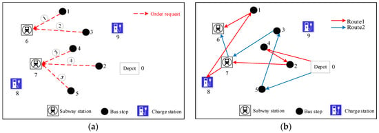
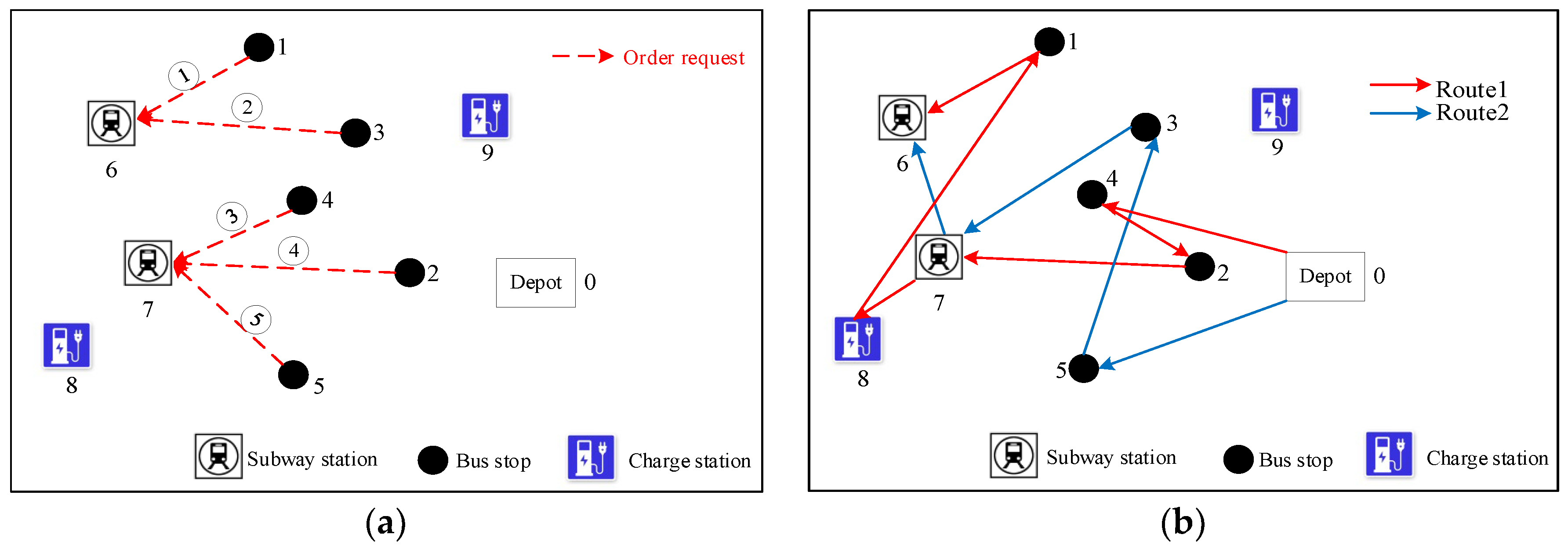
The study area contains a set of EBs ($M$), a set of charging stations ($C$), a set of bus stops ($B$), and a set of subway stations ($Q$). The depot is denoted by 0, and all EBs depart from it. Figure 1 displays an example of a demand-responsive community electric bus connected to subways ($M$ = 2, $Q$ = 2, and $B$ = 5). The pre-given demand matrix contains the requests from the passengers. Each row presents a piece of request information in the demand matrix, including the requested pick-up stop, delivery stop, the earliest possible time in the passenger’s pick-up window, the upper bound of the passenger’s pick-up time window, and the number of passengers. The five requests are shown in the left sub-diagram in Figure 1. Based on demand information, a set of feasible electric bus routes is generated (see the right sub-diagram in Figure 1).

Figure 1. An example of a demand-responsive feeder transit system. (a) Passenger requests from the demand matrix; (b) feasible electric bus routes generated based on the requests.

In order to satisfy the requests, two routes are required, and route information is kept in matrix $S$. The first row lists all the stops for all routes in chronological order in matrix $S$. The request number that is fulfilled at each stop indicated in the first row is listed in the second row. The third row identifies pick-up or delivery operation. If the pick-up operation is 1 and delivery is 2, the route number is finally recorded in the fourth row. In particular, two plus signs (+), used in the second row, represent a virtual request from subway station 7 to the nearest charging station 8, and they record a charging activity. The time distance between 7 and 8 is equal to the map distance plus charging time at 8.

$$\mathit{Demand}=\left[\begin{array}{lllll}1\hfill & 6\hfill & T_s^1\hfill & T_e^1\hfill & n_1\hfill \\ 3\hfill & 6\hfill & T_s^2\hfill & T_e^2\hfill & n_2\hfill \\ 4\hfill & 7\hfill & T_s^3\hfill & T_e^3\hfill & n_3\hfill \\ 2\hfill & 7\hfill & T_s^4\hfill & T_e^4\hfill & n_4\hfill \\ 5\hfill & 7\hfill & T_s^5\hfill & T_e^5\hfill & n_5\hfill \end{array}\right] S=\left[\begin{array}{llllllllllll}4\hfill & 2\hfill & 7\hfill & 7\hfill & 7\hfill & 8\hfill & 1\hfill & 6\hfill & 5\hfill & 3\hfill & 7\hfill & 6\hfill \\ 3\hfill & 4\hfill & 3\hfill & 4\hfill & +\hfill & +\hfill & 1\hfill & 1\hfill & 5\hfill & 2\hfill & 5\hfill & 2\hfill \\ 1\hfill & 1\hfill & 2\hfill & 2\hfill & 1\hfill & 2\hfill & 1\hfill & 2\hfill & 1\hfill & 1\hfill & 2\hfill & 2\hfill \\ 1\hfill & 1\hfill & 1\hfill & 1\hfill & 1\hfill & 1\hfill & 1\hfill & 1\hfill & 2\hfill & 2\hfill & 2\hfill & 2\hfill \end{array}\right]$$

3.2. Problem Assumptions

(1)

The shortest path between any two adjacent stops is used to measure the travel duration.

(2)

The electric bus has a predetermined dwell duration at each stop.

(3)

Passengers only require the pick-up time window in their reservations, while delivery time is affected by transit time on buses.

(4)

The driving range and homogeneity of all electric buses are the same. The electric buses leave after being fully charged.

(5)

All requests are generated at subway stations/bus stops and terminated at bus stops/subway stations. This study does not consider the order requests between subway stations or bus stops.

(6)

The battery state of charge (SOC) is propagated linearly along the route, decreasing proportionally with the travel distance between adjacent stops. Energy consumption is strictly a function of travel distance, and the vehicle’s SOC feasibility is maintained by ensuring it never drops below the safety threshold defined in Equation (22).

3.3. Objective Function

The objective function includes electric bus travel cost, passenger fare discount cost, and charging cost. Electric bus travel cost $C_S$ and charging cost $C_{\mathit{electric}}$ are affected by matrix $S$. Discounted passenger fare cost $C_I$ is influenced by bus departure time $D_0$ at depot and matrix $S$. Therefore, the objective function can be written as

$$F\left(S,D_0\right)=C_S\left(S\right)+C_I\left(S,D_0\right)+C_{\mathit{electric}}\left(S\right)$$

(1)

For clarity, Equation (1) presents only the main cost components, while the complete objective function is given in Equation (26).

(1)

The electric bus travel cost can be expressed as

$$C_S={\mu }_1{\displaystyle \sum _r{\displaystyle \sum _i{d}_{i,i+1}^r}}$$

(2)

where ${\mu }_1$ is a weight coefficient and $d_{i,i+1}^r$ is the shortest travel time on the route $r$ between two neighboring stops.

(2)

The passenger fare discount cost is calculated by the difference between the fare $C_{\mathit{real}}$ that passengers actually paid and basic fare $C_{\mathit{basic}}$, which is defined as the fare discount.

$$C_I=C_{\mathit{basic}}-C_{\mathit{real}}=\phi (T_I-T_{\min })$$

(3)

where $C_{\mathit{basic}}$ is defined as follows.

$$C_{\mathit{basic}}=T_{\min }\cdot \gamma$$

(4)

$$T_{\min }=d_{i_{k2},i_{k2}}^k/V_b$$

(5)

where $T_{\min }$ is minimum travel time; $i_{k1}$ and $i_{k2}$ represent the pick-up and delivery stop of request $k$; $d_{ip1,ip2}^k$ the shortest distance of request $k$; $V_b$ the travel speed; and $\gamma$ represents the fare rate.

$C_{\mathit{real}}$ is the discount fare which passengers actually paid. It can be defined as follows.

$$C_{\mathit{real}}=C_{\mathit{basic}}-\phi (T_I-T_{\min })$$

(6)

$$T_I={\displaystyle \sum _r{\displaystyle \sum _k{\displaystyle \sum _i\left({\delta }_2\left(r,k,i\right)\cdot A_i^r-{\delta }_1\left(r,k,i\right)\cdot B_i^r\right)}}}$$

(7)

where $A_i^r$ is the arrival time of route $r$ at stop $i$; $B_i^r$ the service start time of route $r$ at stop $i$; $n_k$ the passenger number of request $k$; T_I is the actual time spent in transit; and φ represents the discount rate of fares. If request $k$ at its pick-up stop $i$ is served by route $r$, then ${\delta }_1\left(r,k,i\right)$ = 1; otherwise, ${\delta }_1\left(r,k,i\right)$ = 0. If request $k$ at its delivery stop $i$ is served by route $r$, then ${\delta }_2\left(r,k,i\right)$ = 1; otherwise, ${\delta }_2\left(r,k,i\right)$ = 0.

(3)

Arrival time $A_i^r$, departure time $D_i^r$, and service start time $B_i^r$ have the following equality relationships for stop $i$ on electric bus route $r$.

$$A_i^r=D_{i-1}^r+t_{i-1,i}^r$$

(8)

$$D_i^r=B_i^r+t_s$$

(9)

$$B_i^r=\max \left\{A_i^r,T_s^{r,j}\right\}$$

(10)

where $t_s$ is dwell time; $t_{i-1,i}^r$ travel time between $i$ − 1 and $i$; and $T_s^{r,k}$ is the earliest possible time in the passenger’s pick-up window. When electric bus route $r$ arrives at the passenger pick-up stop before $T_s^{r,j}$, the electric bus must wait until $T_s^{r,j}$; otherwise, $A_i^r$ = $B_i^r$. If $i$ is the delivery stop, $A_i^r$ = $B_i^r$.

It uses a nonlinear function to represent the charging process, and it is divided into a three-stage linear segmentation function to facilitate the analysis. When the electric bus enters the charging station, it selects the corresponding charging stage to recharge the battery according to the remaining power $e_d^r$. The charging cost $C_{\mathit{electric}}$ can be expressed as

$$C_{\mathit{electric}}={\displaystyle \sum _r\epsilon \cdot Ch}$$

(11)

where $\epsilon$ represents the electric rate, RMB/minute; $Ch$ is the charging duration in minutes, and is further expressed in Equation (22).

3.4. Constraints and Penalty Functions

In this study, constraints are categorized into two types: hard constraints and soft constraints.

Hard constraints must be satisfied by any feasible solution and define the fundamental feasibility of the routing and charging schedule. Specifically, the request assignment and pairing constraints [Equations (19)–(21)], the charging safety constraint [Equation (22)], and the passenger in-transit time constraint [Equation (14)] are treated as hard constraints. These constraints are strictly enforced and are not subject to relaxation or penalization.

Soft constraints, in contrast, may be temporarily violated during the search process but are incorporated into the objective function via penalty terms to maintain service quality. Specifically, the overload constraint [Equation (13)], the service time-window constraints [Equations (15)–(17)], and the maximum travel-time constraint [Equation (18)] are formulated as soft constraints. Violations of these constraints are quantified by deviation variables $O_i^r$, $\Delta T_k^r$, and $\Delta T_{\max }^r$, respectively, and are penalized through the penalty cost functions $C_{P1}$, $C_{P2}$, and $C_{P3}$ [Equations (23)–(25)]. Consequently, Equations (13) and (15)–(18) serve as the computational basis for penalty cost calculation rather than as absolute feasibility filters.

(1)

Load definition

$L{d}_i^r$ is used to denote passenger flow between stop $i$ and $i$ + 1 on route $r$.

$$L{d}_i^r={\displaystyle \sum _k{\displaystyle \sum _{i^{\prime }=1}^i{\delta }_1\left(r,k,i^{\prime }\right)}}\cdot n_k-{\displaystyle \sum _k{\displaystyle \sum _{i^{\prime }=1}^i{\delta }_2\left(r,k,i^{\prime }\right)}}\cdot n_k,1\le i\le \left|r\right|$$

(12)

where $L{d}_i^r$ denotes the passenger flow (load) between stop $i$ and stop $i$ + 1 on route $r$; ${\delta }_1\left(r,k,i^{\prime }\right)$ and ${\delta }_2\left(r,k,i^{\prime }\right)$ are binary indicators for pick-up and delivery, respectively; $n_k$ is the number of passengers for request $k$; and $\left|r\right|$. represents the total number of stops on route $r$.

(2)

Overload soft constraint

Equation (13) defines the overload amount $O_i^r=\max (0,L{d}_i^r-P)$. The requirement $L{d}_i^r\le P$ is a soft constraint, and any positive overload is penalized by $C_{P2}$ in Equation (24).

$$O_i^r=\max (0,L{d}_i^r-P)$$

(13)

where $P$ is the maximum electric bus load, and $\left|r\right|$ is the number of stops on route $r$ as defined in Equation (12).

(3)

Passenger in-transit time

Equation (14) is a hard constraint. Passenger in-transit time cannot exceed $\sigma$ ($\sigma >1$) times the shortest travel time. The definition of the appropriate restriction for $\forall r,k,i$ is

$$A_{i_{k2}}^r-B_{i_{k1}}^r\le \sigma t_{\min }^k$$

(14)

where $t_{\min }^k$ indicates the quickest travel time between the pick-up and delivery stops of request $k$.

(4)

Service time window soft constraints

Equations (15)–(17) constrain the service time window at stop $i$ for request $k$. Equations (16) and (17) define the time window values for point $i$ as a pick-up or drop-off stop, respectively. The time-window requirement is a soft constraint, and violations are penalized by $C_{P1}$ in Equation (23).

$$\Delta T_k^r=\max (0,T_s^{r,k}-B_k^r,B_k^r-T_e^{r,k}),\forall r,1\le i\le \left|r\right|$$

(15)

$$T_s^{r,k}=\left\{\begin{array}{ll}{T}_s^k\hfill & if{\delta }_1\left(r,k,i\right)=1\hfill \\ D_i^r+t_{\min }^k\hfill & if{\delta }_2\left(r,k,i\right)=1\hfill \end{array}\right.$$

(16)

$$T_e^{r,k}=\left\{\begin{array}{ll}{T}_e^k\hfill & if{\delta }_1\left(r,k,i\right)=1\hfill \\ D_i^r+\sigma t_{\min }^k\hfill & if{\delta }_2\left(r,k,i\right)=1\hfill \end{array}\right.$$

(17)

(5)

Maximum travel time soft constraint

Equation (18) demonstrates the constraint on the longest possible travel time for EBs. The maximum travel-time requirement is a soft constraint, and violations are penalized by $C_{P3}$ in Equation (25).

$$\Delta T_{\max }^r=\max (0,D_{\left|r\right|}^r+t_{\left|r\right|,0}^r-D_0^r-T_{\max })$$

(18)

(6)

Hard logical constraints

Equations (19)–(21) are hard constraints and must be satisfied by all feasible solutions. Equations (19) and (20) state that each request is only executed once and all requests are carried out. Constraint (21), together with (19) and (20), ensures pick-up and delivery pairing. For a given request $k$, if it is assigned to route $r$ (indicated by ${\displaystyle \sum _{\mathrm{i}}{\delta }_1}\left(r,k,i\right)=1$), then the same route must also serve its delivery, which is guaranteed by the implication that ${\displaystyle \sum _{\mathrm{i}}{\delta }_1}\left(r,k,i\right)+{\displaystyle \sum _{\mathrm{i}}{\delta }_2}\left(r,k,i\right)=2$. If request $k$ is not on route $r$, the sum is 0. This pairwise equality ensures that both the pick-up and delivery of the same request are served by the same electric bus.

$${\displaystyle \sum _r{\displaystyle \sum _k{\displaystyle \sum _i{\delta }_1\left(r,k,i\right)=1}}}\hspace{1em}\forall r,k,i$$

(19)

$${\displaystyle \sum _r{\displaystyle \sum _k{\displaystyle \sum _i{\delta }_2\left(r,k,i\right)=1}}}\hspace{1em}\forall r,k,i$$

(20)

$${\displaystyle \sum _i{\delta }_1\left(r,k,i\right)}+{\displaystyle \sum _i{\delta }_2\left(r,k,i\right)}=0 \mathrm{or} 2\hspace{1em}\forall k,i$$

(21)

(7)

Hard charging constraints

Equation (22) is a hard constraint and defines the charging safety threshold and piecewise charging function.

$$Ch=\left\{\begin{array}{cc}\left(E_1-e_d^r\right)/{\lambda }_1+(E_2-E_1)/{\lambda }_2+(E-E_2)/{\lambda }_3\hfill & \underset{¯}{E}\le e_d^r<E_1\hfill \\ \left(E_2-e_d^r\right)/{\lambda }_2+\left(E-E_2\right)/{\lambda }_3\hfill & E_1\le e_d^r<E_2\hfill \\ \left(E-e_d^r\right)/{\lambda }_3\hfill & E_2\le e_d^r<E\hfill \end{array}\right.$$

(22)

Let $E$ be the full battery capacity (in km) and let $\underset{-}{E}$ denote the minimum safety threshold. The battery state of charge (SOC) is represented by the equivalent driving distance $e_d^r$ (km), with SOC = ($e_d^r$/E) × 100%. The charging model in Equation (22) employs a piecewise function to simulate the realistic multi-stage charging characteristics of lithium-ion batteries. Specifically, the thresholds are aligned with standard charging phases: the first stage ($\underset{-}{E}$ ≤ $e_d^r$ ≤ $E_1$) corresponds to the Constant Current (CC) fast-charging phase with the highest charging rate (${\lambda }_1$) due to low internal resistance; the second stage ($E_1$ ≤ $e_d^r$ ≤ $E_2$) represents a transition phase with reduced power; and the third stage ($E_2$ ≤ $e_d^r$ ≤ $E$) corresponds to the Constant Voltage (CV) tapering phase, where the charging rate (${\lambda }_3$) significantly decreases. To avoid dimensional confusion, the charging rates (λ) are expressed in km/min, allowing direct integration with the time-based scheduling model. These rates are derived from the charging power (kW) divided by the average energy consumption rate (kWh/km).

To bridge the gap between abstract distance units and physical battery energy, we explicitly define the mapping relationships as follows:

Let $C_{\mathit{bat}}$ be the battery capacity in kWh and η be the average energy consumption rate in kWh/km. The full driving range $E$ (km) is derived as $E$ = $C_{\mathit{bat}}$/η. Consequently, the state of charge SOC(t) at any time $t$ is physically equivalent to SOC(t) = ${\displaystyle \frac{e_d^r(t)}{E}}$ = ${\displaystyle \frac{e_d^r(t).\eta }{C_{\mathit{bat}}}}$. Similarly, the charging rate λ (km/min) is converted from the physical charging power $P_{\mathit{charge}}$ (kW) by $\lambda ={\displaystyle \frac{P_{\mathit{charge}}}{\eta }}$. This formulation ensures that while the optimization model operates in the spatial domain (km) for routing consistency, it remains strictly consistent with the electrochemical constraints of the battery (kWh).

(8)

Penalty functions

Due to the strong stochasticity of passenger demands in demand-responsive transit, applying strict hard constraints (e.g., strict time windows) can easily lead to infeasible solutions in practice. In summary, although Equations (13) and (15)–(18) appear as constraints in the mathematical formulation, they are implemented as soft penalty mechanisms within the solution approach. During the search process, temporary violations of these constraints are permitted but incur substantial penalties in the objective function through $C_{P1}$, $C_{P2}$, and $C_{P3}$. This design ensures that the algorithm can always explore the solution space without encountering infeasibility, while the penalty structure incentivizes solutions that closely satisfy the operational requirements. Therefore, these constraints function as soft constraints in practice, serving as the basis for penalty cost calculation rather than as rigid feasibility conditions.

$$C_{P1}={\displaystyle \sum _r{\displaystyle \sum _k{n}_k}.g_1\left(\Delta T_r^k\right)}$$

(23)

$$C_{P2}={\displaystyle \sum _r{\displaystyle \sum _i{g}_2}}\left(O_i^r\right)\cdot d_{i,i+1}^r$$

(24)

$$C_{P3}={\displaystyle \sum _r{g}_3}\left(\Delta T_{\max }^r\right)$$

(25)

Note that $C_{P2}$ is only related to matrix $S$, while $C_{P1}$ and $C_{P3}$ are related to $S$ and $D_0$. The objective function can be rewritten as

$$F\left(S,D_0\right)=C_S\left(S\right)+C_I\left(S,D_0\right)+C_{P1}\left(S,D_0\right)+C_{P2}\left(S\right)+C_{P3}\left(S,D_0\right)+C_{\mathit{electric}}\left(S\right)$$

(26)

4. Solution Method

4.1. VNS-SA

Integration problems such as production-distribution and location-routing problems belong to the NP-hard class, making them difficult to solve with exact algorithms (Perl and Daskin [44]). Consequently, heuristic approaches have become more practical and widely adopted (Nagy and Salhi [45]). For example, the simulated annealing algorithm (SA) is a stochastic optimization-seeking algorithm extensively studied for combinatorial optimization problems. VNS-SA has been employed to solve a variety of real-world issues, e.g., the catering system design problem for high-speed railways (Jiang et al. [46]). Meanwhile, SA combined with local search has been applied to vehicle routing problems with time windows (Lin et al. [47]), flow path and location problems (Hamzeei et al. [48]), timetabling problems (Daduna and Voß [49]), and network design optimization (Friesz et al. [50]). These studies demonstrate the capability of SA-based methods in exploring complex search spaces.

It should be noted that the VNS-SA algorithm developed in this study is a metaheuristic approach. The term “optimal” used in the following sections refers to the best-found solution within the heuristic search space, rather than a mathematically proven global optimum of the MINLP. Similarly, the DI1 insertion strategy guarantees the best insertion position (local optimum) for a specific request within the current route, not the global optimality of the entire problem.

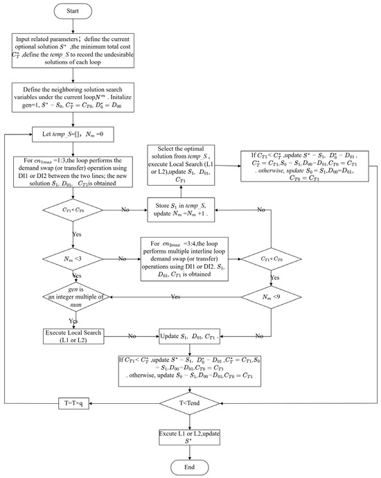
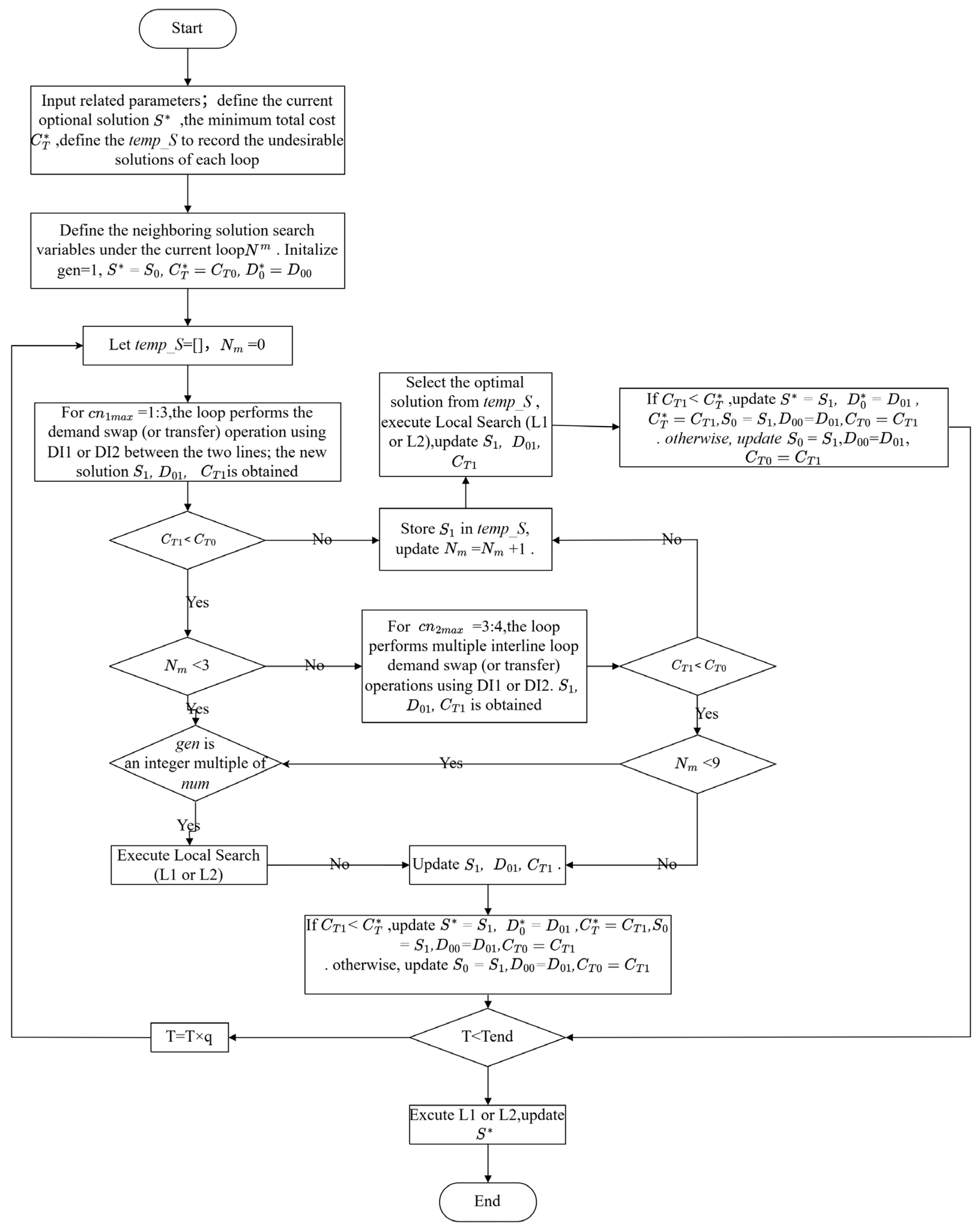
In our VNS-SA, two types of demand swap (or transfer) operations are performed to generate neighboring solutions. The first type operates within two specific routes, utilizing the DI1 or DI2 insertion strategies; this process iterates from 1 to 3. The second type performs multiple inter-route loop demand swap (or transfer) operations between routes using DI1 or DI2; this process iterates from 3 to 4. The requests to be exchanged (or transferred) on a route are still selected under a certain probability.

$del\_P_i=U_i/{\displaystyle \sum U_i}$ denote the selecting probability of request $i$. $U_i=(C_T-C_{T^{\prime }})/n_i$, where $C_{T^{\prime }}$ is the total cost of removed order request $i$ from its current route; $n_i$ denotes the number of passengers corresponding to order request $i$. Algorithm DI1 or DI2 is used to insert them into the target route after selecting the requests. The flow chart of the VNS-SA algorithm is presented in Figure 2.

Figure 2. Flow chart of VNS-SA algorithm. The arrows indicate the logical flow and iteration process of the proposed method.

The flow chart explicitly illustrates the trigger mechanism of the local search strategies (L1 or L2), which are executed when gen is an integer multiple of num. Additionally, all demand swap (or transfer) operations within the neighborhood search loops are executed via the order insertion strategies (DI1 or DI2). The detailed mechanisms of DI1, DI2, L1, and L2 are elaborated in Section 4.4 and Section 4.5.

4.2. Population Initialization

Record the $i$ demand as ${\mathit{Demand}}^i=\left[s_1^i,s_2^i,T_s^i,T_e^i,n_i\right]$ and the $r$th route as $S^r$. Assign requests 1-R to route 1-R and update $S_0=\left[S_0^r,\left[s_1^i;i;1;r\right],\left[s_2^i;i;2;r\right]\right]$ at the matching stage of requests and routes. Then, the remaining requests are allocated one by one according to probability $P_i^r=({\displaystyle \raisebox{1ex}{$1$}\!\left/ \!\raisebox{-1ex}{$V_i^r$}\right.})/{\displaystyle \sum _r\raisebox{1ex}{$1$}\!\left/ \!\raisebox{-1ex}{$V_i^r$}\right.}$, where $V_i^r={\omega }_1\cdot d_{ij}^t+{\omega }_2\cdot d_{ij}^s+{\omega }_3\cdot e_s^r+{\omega }_4\cdot l_r$ is the utility function describing the matching degree between request $i$ and route $r$. The matching degree depends on four factors in this utility function: (1) time distance $d_{ij}^t$ between pick-up stop $s_1^i$ and drop-off stop $s_2^j$ on route $r$, calculated by $d_{ij}^t=\left|{\displaystyle \frac{T_s^i+T_e^i}{2}}-({\displaystyle \frac{T_s^j+T_e^j}{2}}+t_{s_1^j,s_2^j})\right|$; (2) spatial distance $d_{ij}^s$ between $s_1^i$ and $s_2^j$; (3) remaining power $e_s^r$ after request $i$ executed by route $r$; and (4) the length of route $r$.

4.3. Optimized Depot Departure Time Selection

Optimized depot departure time $D_0$ for each route is designed according to the influence relationships among passengers’ pick-up time window, in-transit time, bus travel time, and $D_0$. The time window of the passenger pick-up stop is fixed, while the time window of the drop-off stop depends on the departure time of the corresponding pick-up stop and the passenger’s in-transit time. Depot departure time $D_0$ affects these two types of time windows differently. Then, these two types of time windows are considered separately and denoted as $C_{P11}$ and $C_{P12}$, respectively. Since the influence mechanism of $C_{P12}$ is the same as $C_I$ and they have the same effect on $D_0$, $C_I$ and $C_{P12}$ are considered together and denoted by $C_{IP}$. Based on the above analysis, the change in departure time $D_0$ will have three major effects: (1) The arrival time at the pick-up stops will be affected, which changes $C_{P11}$. (2) Passenger’s in-transit time will be affected, which changes $C_{IP}$. (3) Bus travel time will be affected, which changes $C_{P3}$. Thus, Equation (26) can be rewritten as $F\left(S,D_0\right)=C_S\left(S\right)+C_{IP}\left(S,D_0\right)+C_{P11}\left(S,D_0\right)+C_{P2}\left(S\right)+C_{P3}\left(S,D_0\right)+C_{\mathit{electric}}\left(S\right)$.

(1)

Impacts of $D_0$ on the time window at the pick-up stop

Demand $k$ is assumed to be served on route $r$ and $i_{k1}$ is $k$’s pick-up stop. Then,

$$C_{P11}^{k,r}={\delta }_1\left(r,k,i_{k1}\right)\cdot n_k\cdot g_1\left(B_{i_{k1}}^r\right)$$

(2)

Impacts of $D_0$ on passenger’s in-transit time

Demand $k$ is served on route $r$, and $i_{k1}$ and $i_{k2}$ are $k$’s pick-up and drop-off stops, respectively. Passenger fare discount cost $C_I^{k,r}$ and in-transit time penalty $C_{P12}^{k,r}$ are calculated as follows:

$$C_{IP}^{k,r}=C_I^{k,r}+C_{P12}^{k,r}$$

$$C_I^{k,r}=\phi \cdot n_k\cdot [{\delta }_2\left(r,k,i_{k2}\right)\cdot A_{i_{k2}}^r-{\delta }_1\left(r,k,i_{k1}\right)\cdot B_{i_{k1}}^r]$$

$$C_{P12}^{k,r}={\delta }_1\left(r,k,i_{k2}\right)\cdot n_k\cdot g_1(A_{i_{k2}}-B_{i_{k1}})$$

(3)

Impacts of $D_0$ on bus travel time

Bus route $r$ serves $m$ requests, and 2 × $m$ is the overall number of service stops on it. Bus travel time is defined as $T_k=D_{2m}^r+t_{2m,0}^r-D_0^r$, where $D_{2m}^r$ is the departure time when the bus is at the last stop; $t_{2m,0}^r$ indicates the quickest travel time from the depot to the last stop of route $r$. The definition of the bus travel time penalty $C_{P3}^r$ is

$$C_{P3}^r=g_3(D_{2m}^r+t_{2m,0}^r-D_0^r)$$

$N$ alternative departure times are pre-given in set $D_0^r=\left\{D_0^{r1},\dots ,D_o^{rn},\dots ,D_0^{rN}\right\}$ for route $r$. $C_{P11}^r\left(S,D_o^n\right)$, $C_{IP}^r\left(S,D_o^n\right)$, and $C_{P3}^r$ are calculated for $\forall D_o^n$. The sum of $C_{P11}^r\left(S,D_o^n\right)$, $C_{IP}^r\left(S,D_o^n\right)$, and $C_{P3}^r$ of route $r$ represents the total penalty cost that varies with $D_o^n$. Then, $D_0^{r\ast }$ must be situated on the cumulative curve at an extremal point.

4.4. Order Insertion Strategies

The order insertion strategy refers to inserting a specific request, $ip2\in (ip1,l_r+1]$, and its pick-up point $i_{p1}$ and drop-off stop $i_{p2}$ into a route using a specific method to generate a variety of routing solutions. This section provides two alternate order insertion strategies, denoted as DI1 and DI2. The detailed algorithm steps of these two strategies are summarized in Table 2.

Table 2. Algorithm steps of the proposed order insertion strategies (DI1 and DI2).

Order Insertion Strategy 1 (DI1)
Step 1:	For all $i_{p1}\in [0,l_r],$$i_{p2}\in (ip1,l_r+1],$ calculate total cost $C_T^r$ for route $r$ related to all possible combinations of $i_{p1}$ and $i_{p2}.$
Step 2:	Determine whether it needs to be recharged. If needed, insert virtual requests, calculate charging cost $C_{\mathit{electric}},$ and add it onto $C_T^r.$ Store $C_T^r$ into the set $S\_C_T^r.$
Step 3:	Find the minimal $C_T^r$ in $S\_C_T^r,$ where $i_{p1}$ and $i_{p2}$ are best-found insertion positions within the current route; update $S^r.$
Order Insertion Strategy 2 (DI2)
Step 1:	Determine optimal insertion position $i_{p1}$ based on time distance $d_{i_{p1}j}^t$ for all $j\in [1,l_r].$ Determine whether it needs to be recharged. If needed, insert virtual requests after $i_{p1}$ and calculate charging cost $C_{\mathit{electric}}.$
Step 2:	Iterate all possible positions to determine $i_{p2}$ for all. Determine whether it needs to be recharged. If needed, insert virtual requests after $i_{p2}$ and calculate charging cost $C_{\mathit{electric}}.$
Step 3:	Calculate total cost $C_T^r=C_T^r+C_{\mathit{electric}}$ and store it into set $S\_C_T^r.$
Step 4:	Find the minimal cost in $S\_C_T^r,$ where $i_{p1}$ and $i_{p2}$ are the best-found insertion positions within the current route; update $S^r.$

Design Rationale: DI1 is an exhaustive insertion strategy that aims to find the best feasible pick-up and drop-off positions within the current route structure. It guarantees the locally optimal insertion position at the cost of a higher computational burden. It should be noted that this “optimality” is local to the insertion operation and does not imply the global optimality of the entire MINLP. In contrast, DI2 is a two-stage heuristic designed to reduce the search space. It first determines the pick-up position based on the minimum spatiotemporal distance, and subsequently determines the drop-off position by evaluating the remaining insertion combinations, yielding near-optimal solutions efficiently.

4.5. Local Search Strategies

When the requests performed by each route are determined, the overall cost is reduced by modifying the visit sequence, and two local search (L) methods are developed. The set of requests provided by route $r$ is represented as $\mathit{Demand}\_r$; request $i$ in $\mathit{Demand}\_r$ is denoted as $\mathit{Demand}\_r_i$; and $S^r$ is the electric bus matrix for route $r$.

Design Rationale: L1 executes a “removal-and-reinsertion” mechanism. It iteratively removes a request from the current route matrix and uses DI1 or DI2 to reinsert it into the best-found position. This strategy effectively explores the deep neighborhood of the current solution. L2, on the other hand, constructs the route from scratch. By discarding the current sequence and rebuilding from an empty matrix, L2 provides a larger perturbation to the solution space, which helps the algorithm escape from local optima. The specific algorithmic steps for these two local search strategies (L1 and L2) are detailed in Table 3.

Table 3. Algorithmic steps for the removal-and-reinsertion (L1) and reconstruction (L2) strategies.

L1
Step 1:	Delete all virtual charging requests in $S^r$ to obtain $S{A}^r$ and initialize $i=1$ on route $r$
Step 2:	$\mathrm{Repeat} i_{p1}.$ Delete the columns corresponding to $\mathit{Demand}\_r_i$ from $S{A}^r,$ and update $S{A}^r.$ Execute DI1 or DI2 and reinsert $\mathit{Demand}\_r_i$$\mathrm{into} S{A}^r.$ Determine whether it needs to be recharged. If needed, insert virtual requests after $i_{p1}$$\mathrm{or} i_{p2}.$$\mathrm{Update} S^r.$ $\mathrm{Update} i=i+1$ $\mathrm{until} i=\left|r\right|.$
L2
Step 1:	$\mathrm{Let} S^r$$=\left[\right]; \mathrm{initialize} i=1$ in route $r$
Step 2:	Repeat. $\left(1\right) \mathrm{Insert} \mathit{Demand}\_r_i$$\mathrm{into} S^r$ and execute DI1 or DI2. (2) Determine whether it needs to be recharged. If needed, insert virtual requests after $i_{p1}$ or $i_{p2}.$ (3) Update $i=i+1$ until $i=\left|r\right|$

5. Computational Study

5.1. Experimental Design

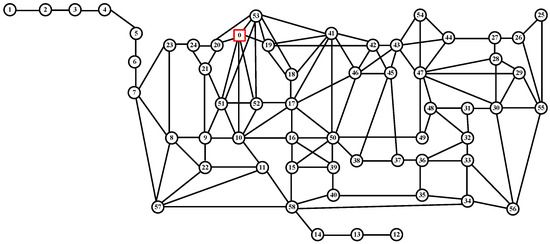
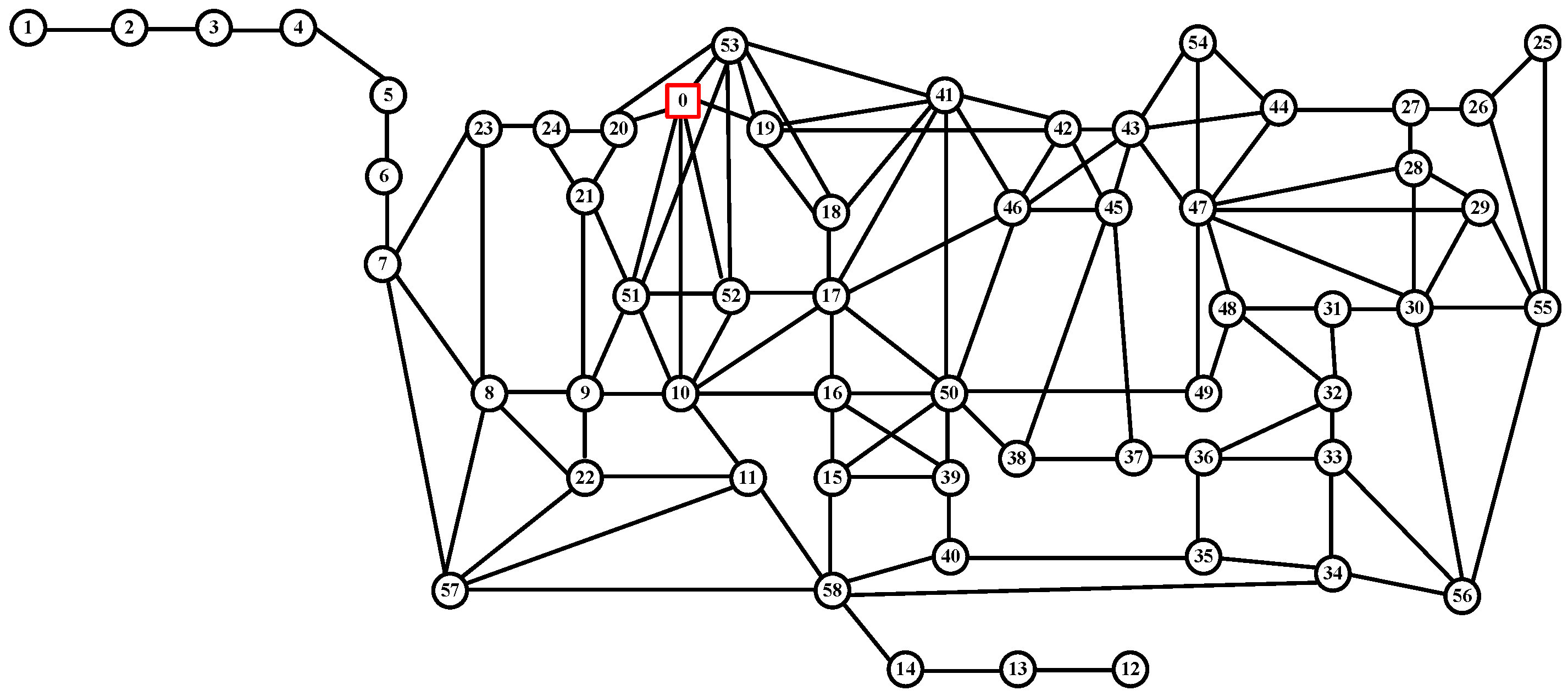
The experiments are based on the real-world road network topology of the Huilongguan community in Beijing (see Figure 3). This network includes 52 bus stops (1–52), six subway stations (53–58), and one depot (0), with five charging stations located at bus stops (Nos. 7, 17, 28, 33, and 38). The shortest distance and shortest travel time between each point are pre-calculated and stored. The electric bus travel speed is considered a constant value.

Figure 3. Experiment network.

To simulate dynamic operations, passenger demands are randomly generated. A random approach is used to generate 68 requests. First, we randomly choose a starting point and an ending point from Nos. 1–52 and 53–58, respectively. Then, use uniform distribution to create random number $P_{\mathit{rand}}$ in the range $\left[0,1\right]$. If $P_{\mathit{rand}}$ > 0.7, the start point is switched with the endpoint, and $P_{\mathit{rand}}\cdot \left(LN-t_w\right)$. The lower limit of time window is generated at random. Here, $\left[0,LN\right]$ stands for the research period, and $LN$ = 300 min. The time window range $t_w$ follows a normal distribution $N\left(10,2^2\right)$, where the second parameter $2^2$ represents the variance (i.e., standard deviation is 2). To ensure physical feasibility, any non-physical negative time window widths generated during the sampling process were handled by truncation (setting to 0) during the data pre-processing stage. Since the algorithm is stochastic, each experimental configuration was independently run five times to ensure statistical reliability, and the average values were reported.

The time window’s upper bound is calculated by $P_{\mathit{rand}}\cdot \left(LN-t_w\right)+t_w$. The scale of the requests is set as $\left[P_{\mathit{rand}}\cdot D_{N\max }\right]$, where $D_{N\max }$ is the maximum persons per request, and $D_{N\max }$ = 5 for our experiments. Repeat the aforementioned operations until 68 order requests are produced. Then, sort the requests in ascending order of $\left(T_s+T_e\right)/2$ to generate matrix Demand.

These additional parameters are crucial: the number of electric buses is $M$ = 8; wait time at stops is $t_s$ = 0.5 min; the electric bus speed is $V_b$ = 20 km/h; ${\mu }_1$ = 9 RMB/km; $\sigma$ = 1.5; the maximum load of an electric bus is $P$ = 11; the maximum electric bus travel time is $T_{\max }$ = 180 min; electric-bus battery capacity is $E$ = 100 km; $\underset{¯}{E}=30\%\cdot E$; $E_1=60\%\cdot E$; $E_2=80\%\cdot E$; ${\lambda }_1$ = 10 km/min; ${\lambda }_2$ = 5 km/min; ${\lambda }_3$ = 1 km/min; $\theta$ = 5 RMB/min; base fare rate $\gamma$ = 0.5 RMB/min; and fare discount rate $\phi$ = 0.1 RMB/min.

Penalty functions $g_1\left(x\right)$, $g_2\left(x\right)$, and $g_3\left(x\right)$ are defined as follows: $\underset{¯}{E}=30\%\cdot E$

$$g_1\left(x\right)=\left\{\begin{array}{cc}3.8\cdot \left(x-T_e^{r,k}\right)\hfill & \hfill \mathrm{x}>T_e^{r,k}\\ 0\hfill & \hfill \mathrm{Otherwise}\end{array}\right.$$

(27)

$$g_2\left(x\right)=\left\{\begin{array}{cc}11\cdot \left(x-P\right)\hfill & \hfill \mathrm{x}>P\\ 0\hfill & \hfill \mathrm{Otherwise}\end{array}\right.$$

(28)

$$g_3\left(x\right)=\left\{\begin{array}{cc}58\cdot \left(x-T_{\max }\right)\hfill & \hfill \mathrm{x}>T_{\max }\\ 0\hfill & \hfill \mathrm{Otherwise}\end{array}\right.$$

(29)

The penalty coefficients in Equations (27)–(29) (3.8, 11, and 58) and the weighting coefficients (${\mu }_1$ = 9 RMB/km, ${\mu }_2$ = 1 RMB/min, $\sigma$ = 1.5) are directly adopted from Xiong [51], who studied a community shuttle optimization problem with a similar network scale and comparable operational characteristics. Since the Huilongguan community network and the operational settings in this study are consistent with those in [51], these values provide a consistent and comparable baseline. The remaining electric-bus-related parameters, including the electricity price $\theta$ = 5 RMB/min, the base fare rate $\gamma$ = 0.5 RMB/min, the fare discount penalty rate $\phi$ = 0.1 RMB/min, the battery capacity $E$ = 100 km, the safety threshold, the intermediate thresholds $E_1=60\%\cdot E$ and $E_2=80\%\cdot E$, and the three-stage charging rates ${\lambda }_1$ = 10 km/min; ${\lambda }_2$ = 5 km/min; and ${\lambda }_3$ = 1 km/min, are scenario-specific settings for the electric bus operation considered in this study. A sensitivity analysis of the termination temperature $T_{\mathit{end}}$ is provided in Section 5.6 (3) to examine the search behavior of the VNS-SA algorithm. Direct sensitivity analysis of the penalty coefficients is left for future work.

5.2. Parameter Configuration

For several parameter configuration methods, the parameters of the suggested algorithm can be modified using techniques like the response surface approach and Taguchi method. The Taguchi parameter calibration method (Sun X et al. [41]) depends on the orthogonal table and signal-to-noise ratio (S/N) to adjust the algorithm’s parameters. S/N is an important statistic for determining how effective the Taguchi method is. The better the value, the larger it is (see Equation (30)).

$$S/N=-10\times \lg ({\displaystyle \frac{1}{a}}{\displaystyle \sum _{i=1}^a{Y}_i^2})$$

(30)

How many orthogonal arrays there are, and the response metrics, are denoted by $a$ and $Y$, respectively. The most efficient factor level has the highest S/N ratio. The common statistical method of mean value analysis is used to determine the best combination of parameters. The main advantage of using this statistical method in the Taguchi method is that the combined results can be represented visually using mean plots. Table 4 shows the parameters and their levels. A five-parameter orthogonal array is designated as L27 (see Table 5).

Table 4. Algorithm parameters and levels.

Algorithm	Algorithm Parameter		Parameter Level
			Level 1	Level 2	Level 3
VNS-SA	A	$T_0$	800	1000	1200
	B	$q$	0.92	0.94	0.96
	C	$num$	10	20	30
	D	$T_{end}$	0.001	0.01	0.1
	E	$\Delta l$	14	18	22

Table 5. Orthogonal array L₂₇.

Experiment	A	B	C	D	E	Target Value	S/N
1	A(1)	B(1)	C(1)	D(1)	E(1)	11,014.47	−80.84
2	A(1)	B(1)	C(1)	D(1)	E(2)	13,543.40	−82.63
3	A(1)	B(1)	C(1)	D(1)	E(3)	6041.20	−75.62
4	A(1)	B(2)	C(2)	D(2)	E(1)	18,430.87	−85.31
5	A(1)	B(2)	C(2)	D(2)	E(2)	15,469.20	−83.79
6	A(1)	B(2)	C(2)	D(2)	E(3)	15,868.85	−84.01
7	A(1)	B(3)	C(3)	D(3)	E(1)	20,351.45	−86.17
8	A(1)	B(3)	C(3)	D(3)	E(2)	12,246.67	−81.76
9	A(1)	B(3)	C(3)	D(3)	E(3)	19,856.93	−85.96
10	A(2)	B(1)	C(2)	D(3)	E(3)	14,155.98	−83.02
11	A(2)	B(1)	C(2)	D(3)	E(2)	21,414.20	−86.61
12	A(2)	B(1)	C(2)	D(3)	E(1)	18,430.87	−85.31
13	A(2)	B(2)	C(3)	D(1)	E(1)	13,227.77	−82.43
14	A(2)	B(2)	C(3)	D(1)	E(2)	15,094.42	−83.58
15	A(2)	B(2)	C(3)	D(1)	E(3)	14,946.86	−83.49
16	A(2)	B(3)	C(1)	D(2)	E(1)	19,301.53	−85.71
17	A(2)	B(3)	C(1)	D(2)	E(2)	16,509.15	−84.35
18	A(2)	B(3)	C(1)	D(2)	E(3)	18,461.69	−85.33
19	A(3)	B(1)	C(3)	D(2)	E(1)	18,474.17	−85.33
20	A(3)	B(1)	C(3)	D(2)	E(2)	17,352.83	−84.79
21	A(3)	B(1)	C(3)	D(2)	E(3)	12,534.47	−81.96
22	A(3)	B(2)	C(1)	D(3)	E(1)	19,301.53	−85.71
23	A(3)	B(2)	C(1)	D(3)	E(2)	18,461.69	−85.33
24	A(3)	B(2)	C(1)	D(3)	E(3)	14,896.93	−83.46
25	A(3)	B(3)	C(2)	D(1)	E(1)	12,543.79	−81.97
26	A(3)	B(3)	C(2)	D(1)	E(2)	9878.94	−79.89
27	A(3)	B(3)	C(2)	D(1)	E(3)	13,526.25	−82.62

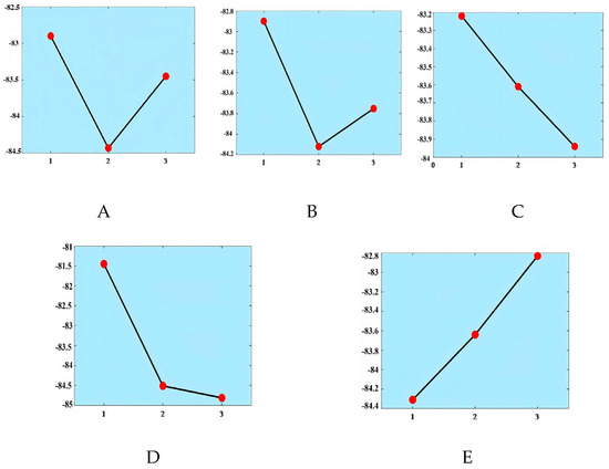
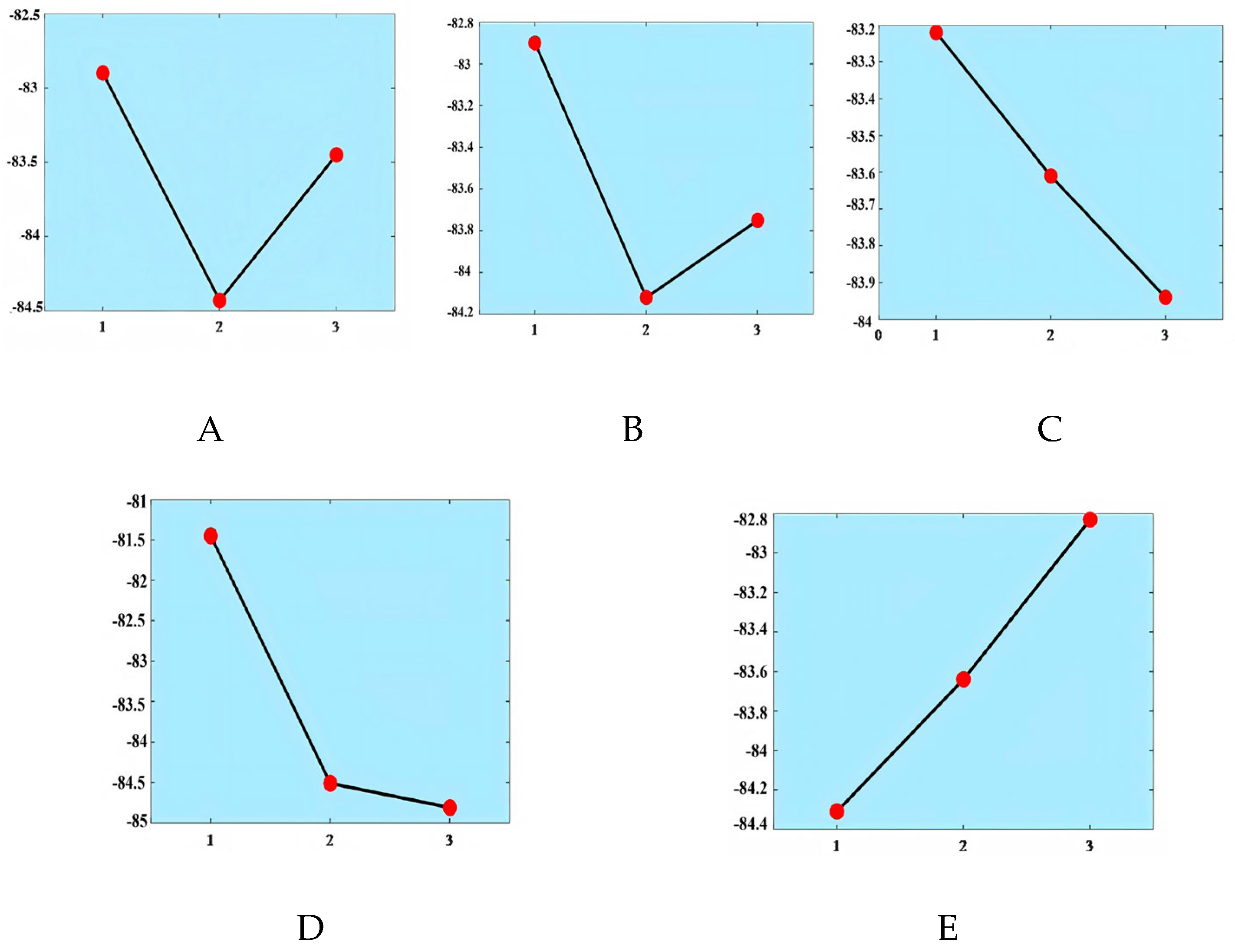
The target value of each experiment is recorded and the mean objective function is calculated (see Table 6). The optimization of parameters requires mean value analysis following the properties of orthogonal experiments. These trials and their impact on the experiment’s goals can be used to predict the best combination of factor levels. Figure 4 presents the S/N ratio associated with the VNS-SA algorithm. The optimal combination of parameters for VNS-SA algorithm is A(1), B(1), C(1), D(1), and E(3).

Table 6. Mean analytical values.

Algorithm	Algorithm Parameter	Mean Value
		1	2	3
VNS-SA	A	−82.90	−84.43	−83.45
	B	−82.90	−84.12	−83.75
	C	−83.22	−83.61	−83.94
	D	−81.45	−84.51	−84.81
	E	−84.31	−83.64	−82.83

Figure 4. Graph illustrating the average impact on the S/N ratio for VNS-SA.

5.3. Best-Found Results

Table 7 shows the tuned parameters of the VNS-SA algorithm. The different combinations of internal algorithms are as follows: $\mathrm{DI}1 + \mathrm{L}1, \mathrm{DI}1 + \mathrm{L}2, \mathrm{DI}2 + \mathrm{L}1$ and $\mathrm{DI}2 + \mathrm{L}2$, and the best-found solutions under different algorithm combinations are compared.

Table 7. Tuned values of parameters.

Parameter	Value
$T_0$	800
$q$	0.92
$num$	10
$T_{end}$	0.001
$\Delta l$	22

(1)

VNS-SA Solution Results

To ensure a fair comparison and fully utilize the algorithm’s potential, all algorithmic parameters were first calibrated to their optimal levels (A(1), B(1), C(1), D(1), E(3)) using the Taguchi method. Therefore, the comparison among the four internal combinations in Table 8 represents an ablation study to analyze the performance trade-offs between different insertion and local search strategies under the optimal parameter settings.

Table 8. Optimization results under each combination of VNS-SA algorithm.

	${\mathit{C}}_{\mathit{S}}$	${\mathit{C}}_{\mathit{I}}$	${\mathit{C}}_{\mathit{P}1}$	${\mathit{C}}_{\mathit{P}2}$	${\mathit{C}}_{\mathit{P}3}$	${\mathit{C}}_{\mathit{e}\mathit{l}\mathit{e}\mathit{c}\mathit{t}\mathit{r}\mathit{i}\mathit{c}}$	$\mathit{F}$	CPU Time (s)
$\mathrm{DI}1+\mathrm{L}1$	2698.65	421.85	667.71	0.00	22.07	51.51	3861.78	1759.34
$\mathrm{DI}1+\mathrm{L}2$	2999.43	502.72	3585.02	0.00	159.78	52.21	7299.17	908.22
$\mathrm{DI}2+\mathrm{L}1$	3004.20	562.13	8892.69	0.00	1733.00	53.14	14,245.16	296.02
$\mathrm{DI}2+\mathrm{L}2$	3553.65	379.37	13,005.02	0.00	4755.68	105.13	21,798.85	228.38

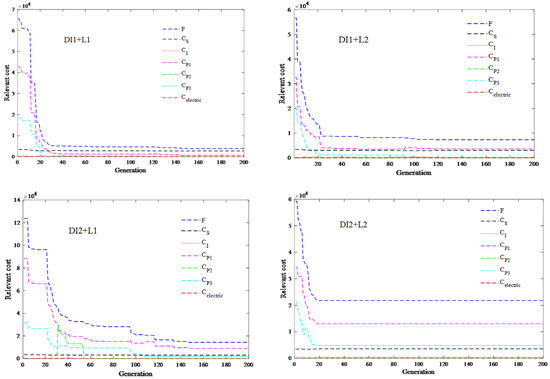
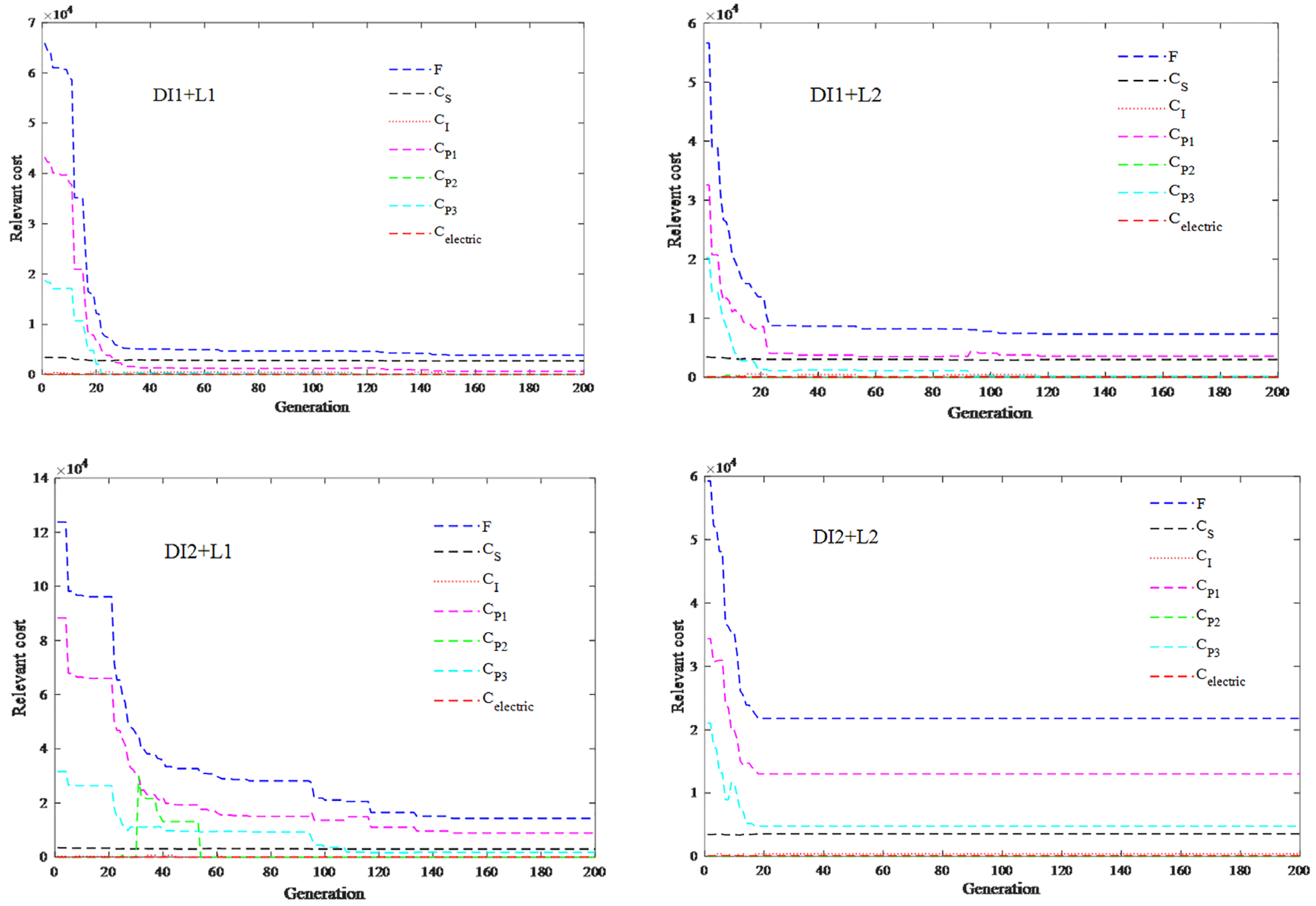
Figure 5 shows that every combination of sub-algorithms converges within a limited number of steps, indicating the stability of the proposed VNS-SA. As shown in Table 8, the combination of DI1 + L1 achieves the best-found objective value among the tested combinations, while DI1 + L2 provides a faster computational time. This reflects the inherent trade-off between solution quality and computational efficiency in the internal operator design. Specifically, the objective function value of DI1 + L1 is smaller than that of DI1 + L2, but its CPU time is twice as long. This is because DI1 exhaustively evaluates potential combinations of pick-up and delivery points, guaranteeing the best insertion position within the current route. In contrast, DI2 adopts a simplified procedure by first selecting the pick-up point, resulting in near-optimal locations with reduced computation. Similar trade-offs are observed between L1 and L2. This ablation study, conducted under the optimal parameter settings (A(1), B(1), C(1), D(1), E(3)), provides a comprehensive understanding of the internal strategy trade-offs.

Figure 5. Iteration curves under each combination of VNS-SA algorithm.

(2)

Optimized Routing and Charging Management

According to the above results, the result of the VNS-SA algorithm under “DI1 + L1” is selected as the best-found solution. Table 9 lists the route optimization results and charging strategy. A total of 68 order requests and nine virtual charging order requests are completed in eight routes, with a total cost of 3861.78 RMB and an operation time of 1759.34 s. Table 9 shows the stop-visiting sequence of electric buses on each line, and the numbers in brackets represent the number of demands responded at each stop.

Table 9. Best-found route and charging strategy.

Route	All the Stops on the Route
1	0 → 43(50) → 57(50) → 21(24) → 54(27) → 4(28) → 3(27) → 53(28) → 17(Charging) → 16(59) → 54(59) → 51(63) → 48(60) → 54(63 and 60) → 36(61) → 56(64) → 17(64) → 0
2	0 → 25(58) → 43(2) → 55(2) → 58(1) → 57(58) → 4(1) → 2(6) → 56(6) → 33(Charging) → 27(30) → 56(30) → 39(32) → 58(32) → 2(34) → 6(39) → 58(34) → 54(39) → 0
3	0 → 58(43) → 40(43) → 55(3) → 9(3) → 57(5, 7) → 9(5) → 35(7) → 34(14) → 56(14) → 46(22) → 17(Charging) → 58(22) → 2(29) → 58(29) → 8(36) → 54(36) → 0
4	0 → 45(45) → 54(45) → 19(10) → 40(19) → 58(10) → 57(19) → 34(23) → 58(23) → 10(35) → 55(35) → 49(37) → 33(Charging) → 58(37) → 13(38) → 54(38) → 26(40) → 34(47) → 58(47) → 57(40) → 40(44) → 49(49) → 54(49, 44) → 46(52) → 17(Charging) → 53(52) → 0
5	0 → 21(20) → 58(20) → 38(4) → 53(4) → 24(8, 12) → 30(9) → 56(8, 9, and 12) → 37(13) → 58(13) → 12(15) → 53(15) → 17(Charging) → 3(26) → 58(26) → 9(42) → 57(42) → 0
6	0 → 22(66) → 33(11) → 55(11, 66) → 57(25) → 36(25) → 23(33) → 53(33) → 39(31) → 38(Charging) → 53(31, 48) → 37(48) → 0
7	0 → 46(54) → 53(54) → 9(56) → 22(55) → 58(53, 55, 56, and 57) → 34(53) → 29(65) → 57(65) → 10(Charging) → 49(68) → 55(67) → 56(68) → 33(Charging) → 0
8	0 → 1(62) → 53(62) → 49(16) → 54(16) → 50(17) → 38(18) → 56(17) → 55(18 and 21) → 28(Charging) → 19(21) → 8(46) → 51(41) → 55(46) → 56(41) → 36(51) → 57(51) → 0

A comprehensive analysis of the influencing factors to obtain the optimized depot departure time is as follows. Unlike traditional fixed-route transit, the EB-DRT system operates on a demand-responsive basis without fixed or predetermined departure times. If a fixed departure time were artificially preset, it would inevitably lead to increased waiting times and excessive in-transit time due to the stochastic passenger time windows. In our model, the depot departure time ($D_0$) directly determines the passenger fare discount cost ($C_I$) and the time window penalty cost ($C_{\mathrm{p}1}$). Based on the best-found solution in Table 9, these two time-related cost components account for 421.85 RMB and 667.71 RMB, respectively, which constitute a significant portion of the total system cost (3861.78 RMB). Therefore, the endogenous optimization of $D_0$ is mathematically essential for minimizing these time-related costs and achieving a near-optimal system cost. Table 10 presents the optimized depot departure times and the corresponding electric bus assignments under different time horizons.

Table 10. Optimized depot departure time.

	0	10 min	20 min	30 min	40 min	50 min
One hour	EBs 2, 5, and 8		EBs 3 and 6		EB 4
Two hours				EB 1
Three hours			EB 7

5.4. Solution Quality and Stability Validation

5.4.1. Exact-Solver Benchmark on Small Instances

To evaluate the quality of VNS-SA on small-scale instances, we applied the Gurobi exact solver to 10-request and 20-request sub-instances drawn from the same demand distribution as the full 68-request instance. Because the full joint routing-and-assignment problem is NP-hard, we fixed the vehicle-request assignment y to VNS-SA’s solution and solved the remaining routing subproblem to optimality. The comparison is therefore conducted under a common objective $C_S$ + $C_{P1}$ + $C_{P2}$, which excludes the charging cost and other components that are not modeled in the Gurobi benchmark.

In Table 11, the “Objective” column reports the common objective value ($C_S$ + $C_{P1}$ + $C_{P2}$) for both solvers under the same fixed vehicle-request assignment, ensuring an apples-to-apples comparison. It should be noted that VNS-SA uses the complete objective function in Equation (26) during its search, but its final solution is re-evaluated under this common objective for comparison with Gurobi. Under this common objective, VNS-SA achieves a gap of 11.90% (10 requests) and 30.20% (20 requests) compared with Gurobi. The increasing gap with problem size reflects the growing difficulty of the routing subproblem. Importantly, this gap is not the global optimality gap of the full MINLP; it is only the gap for the routing subproblem under a fixed vehicle-request assignment. Therefore, the gap may partly reflect this structural difference rather than pure algorithmic inferiority.

Table 11. Gurobi vs. VNS-SA results for the routing subproblem under fixed vehicle-request assignment.

Instance	Requests	Vehicles	Solver	Objective	Time (s)	Gap
Small-1	10	3	Gurobi (fixed y)	1149.59	24.5	—
Small-1	10	3	VNS-SA	1286.33	~1	11.90%
Small-2	20	5	Gurobi (fixed y)	2010.38	104.8	—
Small-2	20	5	VNS-SA	2617.32	~3	30.20%

5.4.2. Reproducibility Analysis

To assess the reproducibility of VNS-SA, ten independent runs with fixed random seeds (20250001–20250010) were performed on the 10-request and 20-request instances. The statistical results of these ten independent runs are summarized in Table 12.

Table 12. Statistical results of ten independent VNS-SA runs with fixed random seeds.

Instance	Mean	Std	CV	Min	Max
10 requests	1071.8	170.84	15.94%	839.87	1323.08
20 requests	1941.6	228.42	11.76%	1673.69	2405.29

The coefficient of variation decreases from 15.94% (10 requests) to 11.76% (20 requests), confirming that VNS-SA achieves better stability in larger instances. The relatively high CV on the small instance is a well-documented characteristic of stochastic local search algorithms, where the random initial-solution ordering and neighborhood selection have a proportionally larger impact.

The VNS-SA parameters were set to $T_0=800$, $q=0.92$, $num=10$, $T_{\mathit{end}}=0.001$, and $\Delta l=22$, as calibrated by the Taguchi method (Section 5.2). All experiments were performed in MATLAB R2021a with Gurobi 10.1.1 on a Dell computer running Windows 10, configured with a 2.40 GHz CPU and 4 GB of RAM.

5.5. Analysis of Departure Time Optimization

To validate the necessity of treating the depot departure time ($D_0$) as a decision variable, we conducted a comparative analysis between the proposed optimization model and strategies with fixed departure times. The evaluation is based on a representative subset of 41 requests selected from the full test set of 68 cases, ensuring computational tractability while preserving statistical representativeness. Specifically, the 41 requests were selected using a distance-based stratified sampling strategy. The 68 requests in the full test set were first sorted in ascending order by their shortest travel distance. The top 20 requests with the shortest distances and the bottom 21 requests with the longest distances were retained, while the 27 requests with intermediate distances were excluded. This selection strategy ensures that the subset covers both short-distance and long-distance scenarios, thereby providing a comprehensive evaluation of the algorithm’s performance across different distance ranges.

For the baseline scenarios, we simulated common operational practices by setting $D_0$ to fixed intervals of 30, 60, and 90 min—values that reflect typical rigid scheduling policies in real-world demand-responsive transit systems. Additionally, to establish a statistically grounded reference, we introduced a mean departure time strategy ($\stackrel{-}{D_0}$), calculated as the average of the optimized departure times obtained by the proposed algorithm across multiple independent runs with different random seeds. This value represents an empirically derived “central tendency” of the optimized solution space.

The detailed results are presented in Table 13. As shown, fixing the departure time leads to a significant deterioration in system performance. Specifically:

Table 13. Comparison of system performance between optimized and fixed departure time strategies.

${\mathit{D}}_0$ (min)	${\mathit{C}}_{\mathit{S}}$	${\mathit{C}}_{\mathit{I}}$	${\mathit{C}}_{\mathit{P}1}$	${\mathit{C}}_{\mathit{P}2}$	${\mathit{C}}_{\mathit{P}3}$	${\mathit{C}}_{\mathbf{electric}}$	$\mathit{F}$	${\mathit{C}}_{\mathit{P}}$	${\mathit{C}}_{\mathit{P}}/\mathit{F}$ (%)
30	4296.20	19.26	2493.41	207.24	6147.62	206.92	13,370.65	8848.27	66%
60	4210.61	17.44	4950.96	0	1756.64	52.89	10,988.54	6707.6	61%
90	4569.65	16.32	8932.74	0	0	79.03	13,597.74	8932.74	66%
$\stackrel{-}{D_0}$	4932.97	12.72	1531.29	0	0	211.22	6688.20	1531.29	23%
$\mathrm{Optimized} D_0$	3555.72	11.21	714.81	0	0	150.96	4432.70	714.81	16%

(1)

Surge in Penalty Costs: When $D_0$ is fixed (e.g., at 30 min), the penalty cost ($C_P$) accounts for a disproportionately large share of the total system cost ($F$). This indicates that rigid departure schedules force the system to incur massive penalties due to time window violations or capacity overloads, as vehicles cannot adjust their start times to match demand peaks effectively.

(2)

Total Cost Reduction: By optimizing $D_0$, the total system cost ($F$) drops to 4432.70, which is significantly lower than the fixed scenarios.

(3)

Operational Efficiency: The optimized schedule also achieves a lower operational cost compared to fixed baselines, suggesting that flexible departure times allow for more efficient route planning and charging scheduling.

In conclusion, the comparison demonstrates that optimizing the departure time is not merely an auxiliary improvement but a critical factor in ensuring the feasibility and economic viability of the DRT service. It effectively transforms an infeasible or high-penalty problem into a well-balanced operational plan. Even the statistically averaged strategy ($\stackrel{-}{D_0}$) significantly outperforms rigid fixed intervals, yet the real-time optimized $D_0$ achieves the lowest system cost, highlighting the value of dynamic scheduling.

5.6. Sensitivity Analysis

(1)

EB Fleet Size

This section performs a sensitivity analysis on the fleet size of electric buses to reveal its effect on average route length and charging management. Here, the VNS-SA algorithm with “DI1 + L1” is chosen to run the model under five different fleet sizes (M = 6, 7, 8, 9, and 10), and other parameters are constant. For each fleet size, the model was run 10 times, and the average values were taken.

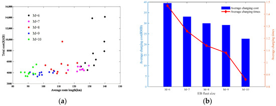
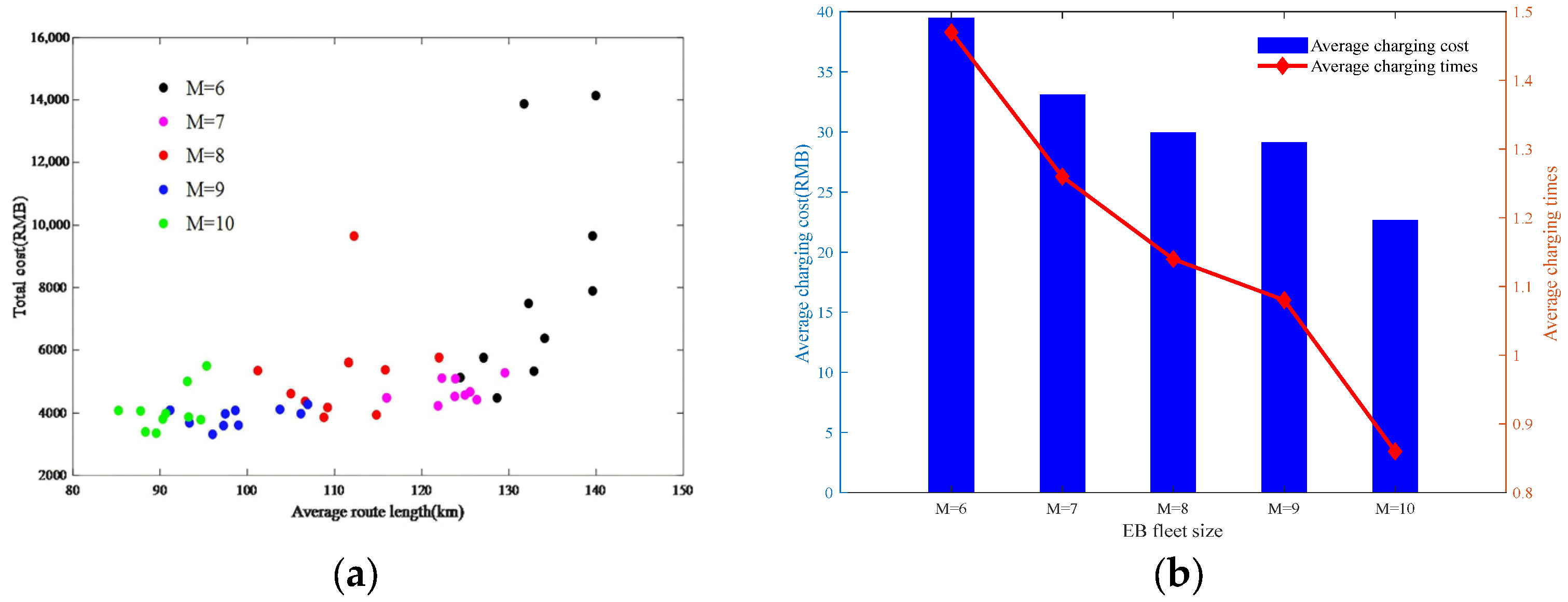
Figure 6 presents the results on the average route length, charging costs, and charging times. The set of scatter plots is constructed to represent the relationship between the average route length and the total cost for different fleet size conditions (see Figure 6a), and the average route length decreases as the fleet size increases. Figure 6b demonstrates that the average charging cost per route and the number of charges decrease accordingly as the fleet size increases.

Figure 6. Effect of the fleet size on optimization results. (a) Scatter plots of average route length versus total cost for different fleet sizes; (b) average charging cost and number of charging times under different fleet sizes.

(2)

Request size

The optimization performance of VNS-SA is compared using the combination of DI1 + L1. Twelve scenarios under different request sizes are generated and denoted as 1a–4c in Table 14. Scenarios 1–4 include 50, 70, 90, and 110 requests, respectively. The widths of the time windows for scenarios a, b, and c are generated at random from normal distributions with variances $N\left(5,1^2\right)$, $N\left(10,2^2\right)$, and $N\left(15,3^2\right)$, respectively, where the second parameter represents the variance. Consistent with Section 5.1, any generated negative values are handled by truncation (setting to 0). Each scenario is solved five times using VNS-SA to ensure statistical reliability, and the following metrics are recorded: minimum objective function value, average objective function value, average charging times, and average running time. The average values are reported in Table 14, which provides solid statistical evidence for the performance of the proposed VNS-SA.

Table 14. Comparison of VNS-SA optimization results under different order requests.

	VNS-SA
	${\mathit{C}}_{\mathit{T}}^{\ast }$	$\overline{{\mathit{C}}_{\mathit{T}}}$	Charging Times	Running Time (s)
1a	2510.77	2606.41	7	559.3
1b	2696.66	3441.55	6	662.19
1c	2777.59	2933.33	8	697.46
2a	6383.04	6561.64	9	1568.16
2b	6741.28	7885.11	9	2012.1
2c	7018.28	7204.51	9	1984.08
3a	11,605.15	12,863.99	13	9569.72
3b	10,792.77	13,103.51	12	9508.87
3c	8496.81	10,926.57	12	5957.83
4a	23,031.24	24,110.18	13	16,858.2
4b	20,549.13	22,799.15	13	12,852.07
4c	19,360.02	20,231.67	15	10,974.56

When the scenario changes from “1” to “4”, the problem size increases continuously, and the minimum and average objective function values ($C_T^{\ast }$ and $\overline{C_T}$) and running time of the VNS-SA algorithm increase significantly (see Table 14). However, it is noted that the trend is not strictly monotonic as the time-window constraint is relaxed from “a” to “c”. Specifically, for the 50- and 70-request cases, the minimum objective values ($C_T^{\ast }$) slightly increase from case “a” to case “c”. This can be attributed to the interaction between the vehicle routing cost and the time window penalty cost. When the time window is significantly relaxed, the algorithm may explore routes that minimize travel distance but yield slightly higher time window penalties due to the stochastic search paths and penalty weights, resulting in a local increase in the minimum objective value.

When the problem size increases, the number of charging events increases because more charging activities are needed to enable the electric bus to complete all the requests. Based on the above analysis, it is necessary to consider the scale of the problem, the degree of emphasis on the solution result, and the running time in practice. Appropriate choices of different internal algorithm combinations should be made to achieve a better trade-off between the optimized result and computational time.

(3)

Sensitivity of the VNS-SA Algorithm to the Termination Temperature

Because the penalty coefficients and weighting coefficients are directly adopted from Xiong [51], this study does not re-calibrate them. It should be emphasized that the following analysis does not vary the penalty coefficients in Equations (27)–(29). Instead, it examines the sensitivity of the VNS-SA algorithm to the termination temperature $T_{T\mathrm{end}}$. $T_{T\mathrm{end}}$ is an algorithmic parameter of the simulated annealing acceptance rule. A lower $T_{T\mathrm{end}}$ makes the algorithm more selective when accepting new solutions, which may indirectly affect whether solutions with higher penalty costs are retained; a higher $T_{T\mathrm{end}}$ relaxes the acceptance criterion. Therefore, $T_{T\mathrm{end}}$ controls the search behavior of VNS-SA and does not represent the relative weights of the penalty terms in the objective function.

The mean objective values corresponding to $T_{T\mathrm{end}}$ = 0.001, 0.01, and 0.1 are 12,201.90, 16,933.64, and 17,679.58 (calculated from the orthogonal experimental results in Table 5), respectively. The objective value increases sharply when $T_{T\mathrm{end}}$ rises from 0.001 to 0.01 (+38.8%), but exhibits only marginal further change from 0.01 to 0.1 (+4.4%). This behavior should be interpreted as the sensitivity of the VNS-SA search process to the termination temperature, rather than as a direct sensitivity of the model to the penalty coefficients.

These findings provide algorithmic guidance for implementing VNS-SA. Setting $T_{T\mathrm{end}}$ too high may retain low-quality solutions, whereas an excessively low value may over-restrict solution acceptance and reduce search diversity. The calibrated value $T_{T\mathrm{end}}$ = 0.001 used in this study lies in the low-value region and yields stable convergence on the tested instances. Since the penalty coefficients are inherited from Xiong [51], a direct sensitivity analysis of these coefficients is not conducted here and is left for future work.

(4)

Validation strategy and limitations

The above Subsections (1)–(3) examined the sensitivity of fleet size, request size, and the termination temperature $T_{T\mathrm{end}}$, respectively. In addition to these specific analyses, the overall validation strategy of this study is summarized as follows. The main contribution of this paper is the integrated EB-DRT model with endogenous departure time and nonlinear charging, rather than a new metaheuristic. The VNS-SA framework is adopted from the existing literature and adapted to this problem. Therefore, the validation focuses on three aspects: (1) whether the model can be solved by the proposed VNS-SA; (2) whether the internal operators (DI1/DI2, L1/L2) exhibit the expected trade-offs; and (3) whether the algorithm parameters are well calibrated. For this purpose, the Taguchi method was used for parameter tuning, and an ablation study was conducted among four internal operator combinations. The number of independent runs and the averaged results are reported in Section 5.4.1 and Section 5.4.2. The signal-to-noise ratios reported in Table 5 and Figure 4 provide additional statistical evidence for the internal consistency and convergence behavior of the proposed VNS-SA. It should be noted that external algorithm comparison and the full MINLP exact optimality gap is not quantified; only a small-instance routing subproblem benchmark with fixed vehicle-request assignment is provided in Section 5.4.1, and they are left for future work. The sensitivity analysis in Section 5.6 (3) concerns the algorithmic parameter $T_{T\mathrm{end}}$, not the penalty coefficients. Direct variation in the penalty coefficients in Equations (27)–(29) is not performed in this study and is left for future work.

6. Conclusions

In this study, we investigated demand-responsive feeder transit services connecting large communities and subway stations. We proposed an integrated routing and charging optimization model with endogenous depot departure time selection, where $D_0$ is treated as a decision variable rather than a fixed input. The model incorporates a nonlinear three-stage piecewise charging function and soft penalty functions for time windows, overload, and maximum travel time. The model was solved by a VNS-SA algorithm with DI1/DI2 insertion strategies and L1/L2 local search strategies, and the algorithm parameters were calibrated by the Taguchi method.

Numerical experiments were conducted on the real-world road network topology of the Huilongguan community in Beijing. Under the best-found solution, 68 order requests and nine virtual charging requests were completed in eight routes, with a total cost of 3861.78 RMB and a CPU time of 1759.34 s. DI1 + L1 achieved the best-found objective value among the tested operator combinations, while DI1 + L2 provided faster computation. The time-related costs $C_I$ and $C_{\mathrm{p}1}$ were 421.85 RMB and 667.71 RMB, respectively, providing evidence for the importance of endogenous departure time optimization. In the 41-request comparison, fixed departure times of 30, 60, and 90 min led to total costs between 10,988 and 13,598 RMB, whereas the optimized departure time reduced the total cost to 4432.70 RMB.

Several limitations should be noted. The full MINLP exact optimality gap was not quantified; only a small-instance routing subproblem benchmark with fixed vehicle-request assignment was provided. No external metaheuristic comparison was conducted. The sensitivity analysis focused on the algorithmic termination temperature $T_{T\mathrm{end}}$, not on the penalty coefficients in Equations (27)–(29). The proposed algorithm is designed for offline planning, and full charging before departure is a simplification. Future research will focus on multi-objective optimization, dynamic traffic networks, direct sensitivity analysis of penalty coefficients, partial charging and opportunity charging strategies, and comparisons with other metaheuristics and exact solvers.

References

- Yan, Y.; Liu, Z.; Bie, Y. Performance Evaluation of Bus Routes Using Automatic Vehicle Location Data. J. Transp. Eng. 2016, 142, 04016029. [Google Scholar] [CrossRef] [Scilit]
- Cayford, R.; Yim, Y. Personalized Demand-Responsive Transit Service; Institute of Transportation Studies, UC Berkeley: Berkeley, CA, USA, 2004. [Google Scholar]
- Wang, J.; Kang, L.; Liu, Y. Optimal scheduling for electric bus fleets based on dynamic programming approach by considering battery capacity fade. Renew. Sustain. Energy Rev. 2020, 130, 109978. [Google Scholar] [CrossRef] [Scilit]
- Houbbadi, A.; Trigui, R.; Pelissier, S. Optimal Scheduling to Manage an Electric Bus Fleet Overnight Charging. Energies 2019, 12, 2727. [Google Scholar] [CrossRef] [Scilit]
- Gao, Z.; Lin, Z.; Laclair, T.J. Battery capacity and recharging needs for electric buses in city transit service. Energy 2017, 122, 588–600. [Google Scholar] [CrossRef] [Scilit]
- Chandra, S.; Quadrifoglio, L. A model for estimating the optimal cycle length of demand responsive feeder transit services. Transp. Res. Part B Methodol. 2013, 51, 1–16. [Google Scholar] [CrossRef] [Scilit]
- Ganji, M.; Kazemipoor, H.; Hadji Molana, S.M.; Sajadi, S.M. A green multi-objective integrated scheduling of production and distribution with heterogeneous fleet vehicle routing and time windows. J. Clean. Prod. 2020, 259, 120824. [Google Scholar] [CrossRef] [Scilit]
- Peled, I.; Lee, K.; Jiang, Y. Online Predictive Optimization Framework for Stochastic Demand-Responsive Transit Services. arXiv 2019, arXiv:1902.09745. [Google Scholar]
- Sun, B.; Wei, M.; Yang, C. Personalised and Coordinated Demand-Responsive Feeder Transit Service Design: A Genetic Algorithms Approach. Future Internet 2018, 10, 61. [Google Scholar] [CrossRef] [Scilit]
- Zhang, L.; Chen, T.; Yu, B. Suburban Demand Responsive Transit Service With Rental Vehicles. IEEE Trans. Intell. Transp. Syst. 2021, 22, 2391–2403. [Google Scholar] [CrossRef] [Scilit]
- Tao, C.; Zhang, B. Optimal Routing and Charging of an Electric Vehicle Fleet for High-Efficiency Dynamic Transit Systems. IEEE Trans. Smart Grid 2016, 9, 3563–3572. [Google Scholar] [CrossRef] [Scilit]
- Yao, C.; Chen, S.; Salazar, M. Joint Routing and Charging Problem of Electric Vehicles With Incentive-Aware Customers Considering Spatio-Temporal Charging Prices. IEEE Trans. Intell. Transp. Syst. 2023, 24, 12215–12226. [Google Scholar] [CrossRef] [Scilit]
- Song, C.; Chen, S.; Wang, H. An Optimization Model for the Demand-Responsive Transit With Non-Fixed Stops and Multi-Vehicle Type. IEEE Access 2023, 11, 92647–92659. [Google Scholar] [CrossRef] [Scilit]
- Tong, L.; Zhou, L.; Liu, J. Customized bus service design for jointly optimizing passenger-to-vehicle assignment and vehicle routing. Transp. Res. Part C Emerg. Technol. 2017, 85, 451–475. [Google Scholar] [CrossRef] [Scilit]
- Yan, X.; Zhao, X.; Han, Y. Mobility-on-demand versus fixed-route transit systems: An evaluation of traveler preferences in low-income communities. Transp. Res. Part A Policy Pract. 2021, 148, 481–495. [Google Scholar] [CrossRef] [Scilit]
- Li, X.; Wang, T.; Xu, W. A novel model and algorithm for designing an eco-oriented demand responsive transit (DRT) system. Transp. Res. Part E Logist. Transp. Rev. 2022, 157, 102556. [Google Scholar] [CrossRef] [Scilit]
- Amirgholy, M.; Gonzales, E.J. Demand responsive transit systems with time-dependent demand: User equilibrium, system optimum, and management strategy. Transp. Res. Part B Methodol. 2016, 92, 234–252. [Google Scholar] [CrossRef] [Scilit]
- Galarza Montenegro, B.D.; Sörensen, K.; Vansteenwegen, P. A large neighborhood search algorithm to optimize a demand-responsive feeder service. Transp. Res. Part C Emerg. Technol. 2021, 127, 103102. [Google Scholar] [CrossRef] [Scilit]
- Wang, Z.; Yu, J.; Hao, W. Joint Optimization of Running Route and Scheduling for the Mixed Demand Responsive Feeder Transit With Time-Dependent Travel Times. IEEE Trans. Intell. Transp. Syst. 2021, 22, 2498–2509. [Google Scholar] [CrossRef] [Scilit]
- Sun, B.; Wei, M.; Zhu, S. Optimal Design of Demand-Responsive Feeder Transit Services with Passengers’ Multiple Time Windows and Satisfaction. Future Internet 2018, 10, 30. [Google Scholar] [CrossRef] [Scilit]
- Hou, Y.; Liu, T.; Hu, H.; Du, B. Optimal Routing Design of Demand-Responsive Feeder Transit in the Era of Mobility as a Service. In Proceedings of the 2022 IEEE 25th International Conference on Intelligent Transportation Systems (ITSC), Macau, China, 8–12 October 2022. [Google Scholar]
- Jin, W.; Ren, J.; Wu, W. Demand Responsive Feeder Transit Scheduling with Flexible Service Quality. In Proceedings of the 2020 IEEE 5th International Conference on Intelligent Transportation Engineering (ICITE), Beijing, China, 11–13 September 2020. [Google Scholar]
- Nickkar, A.; Lee, Y.-J. Dynamic Demand-Responsive Feeder Bus Network Design for a Short Headway Trunk Line. Algorithms 2023, 16, 506. [Google Scholar] [CrossRef] [Scilit]
- Kancharla, S.R.; Ramadurai, G. Electric Vehicle Routing Problem with Non-Linear Charging and Load-Dependent Discharging. Expert Syst. Appl. 2020, 160, 113714. [Google Scholar] [CrossRef] [Scilit]
- Gairola, P.; Nezamuddin, N. Optimization framework for integrated battery electric bus planning and charging scheduling. Transp. Res. Part D Transp. Environ. 2023, 118, 103697. [Google Scholar] [CrossRef] [Scilit]
- Zhang, L.; Wang, S.; Qu, X. Optimal electric bus fleet scheduling considering battery degradation and non-linear charging profile. Transp. Res. Part E Logist. Transp. Rev. 2021, 154, 102445. [Google Scholar] [CrossRef] [Scilit]
- Hu, H.; Du, B.; Liu, W.; Perez, P. A joint optimisation model for charger locating and electric bus charging scheduling considering opportunity fast charging and uncertainties. Transp. Res. Part C Emerg. Technol. 2022, 141, 103732. [Google Scholar] [CrossRef] [Scilit]
- Avishan, F.; Yanıkoğlu, İ.; Alwesabi, Y. Electric bus fleet scheduling under travel time and energy consumption uncertainty. Transp. Res. Part C Emerg. Technol. 2023, 156, 104357. [Google Scholar] [CrossRef] [Scilit]
- Hiermann, G.; Puchinger, J.; Ropke, S. The Electric Fleet Size and Mix Vehicle Routing Problem with Time Windows and Recharging Stations. Eur. J. Oper. Res. 2016, 252, 995–1018. [Google Scholar] [CrossRef] [Scilit]
- Wang, Y.; Liao, F.; Lu, C. Integrated optimization of charger deployment and fleet scheduling for battery electric buses. Transp. Res. Part D Transp. Environ. 2022, 109, 103382. [Google Scholar] [CrossRef] [Scilit]
- Liu, W.L.; Gong, Y.J.; Chen, W.N. Coordinated Charging Scheduling of Electric Vehicles: A Mixed-Variable Differential Evolution Approach. IEEE Trans. Intell. Transp. Syst. 2019, 21, 5094–5109. [Google Scholar] [CrossRef] [Scilit]
- Liu, Y.; Cheng, C.; Shi, H. A Two-Stage Approach With a Departure Time Based Solution Representation for Electric Bus Vehicle Scheduling. IEEE Access 2022, 10, 12799–12811. [Google Scholar] [CrossRef] [Scilit]
- Mishra, S.; Mondal, A.; Mondal, S. A Multi-Objective Optimization Framework for Electric Vehicle Charge Scheduling with Adaptable Charging Ports. IEEE Trans. Veh. Technol. 2023, 72, 5702–5714. [Google Scholar] [CrossRef] [Scilit]
- Shao, S.; Sartipizadeh, H.; Gurta, A. Scheduling EV Charging Having Demand With Different Reliability Constraints. IEEE Trans. Intell. Transp. Syst. 2023, 24, 11018–11029. [Google Scholar] [CrossRef] [Scilit]
- Tan, M.; Ren, Y.; Pan, R. Fair and Efficient Electric Vehicle Charging Scheduling Optimization Considering the Maximum Individual Waiting Time and Operating Cost. IEEE Trans. Veh. Technol. 2023, 72, 9808–9820. [Google Scholar] [CrossRef] [Scilit]
- Qian, L.P.; Zhou, X.; Yu, N.; Wu, Y. Electric Vehicles Charging Scheduling Optimization for Total Elapsed Time Minimization. In Proceedings of the 2020 IEEE 91st Vehicular Technology Conference (VTC2020-Spring), Antwerp, Belgium, 25–28 May 2020. [Google Scholar]
- Olsen, N.; Kliewer, N. Location Planning of Charging Stations for Electric Buses in Public Transport Considering Vehicle Scheduling: A Variable Neighborhood Search Based Approach. Appl. Sci. 2022, 12, 3855. [Google Scholar] [CrossRef] [Scilit]
- Jiang, M.; Zhang, Y.; Zhang, Y. Multi-Depot Electric Bus Scheduling Considering Operational Constraint and Partial Charging: A Case Study in Shenzhen, China. Sustainability 2022, 14, 255. [Google Scholar] [CrossRef] [Scilit]
- Garaix, T.; Artigues, C.; Feillet, D. Vehicle routing problems with alternative paths: An application to on-demand transportation. Eur. J. Oper. Res. 2010, 204, 62–75. [Google Scholar] [CrossRef] [Scilit]
- Sun, X.; Liu, S. Research on Route Deviation Transit Operation Scheduling-A Case Study in Suburb No. 5 Road of Harbin. Sustainability 2022, 14, 633. [Google Scholar] [CrossRef] [Scilit]
- Sun, X.; Shi, Z.; Zhu, J. Multiobjective design optimization of an IPMSM for EVs based on fuzzy method and sequential taguchi method. IEEE Trans. Ind. Electron. 2020, 68, 10592–10600. [Google Scholar] [CrossRef] [Scilit]
- Gong, L.; Cao, W.; Liu, K. Demand responsive charging strategy of electric vehicles to mitigate the volatility of renewable energy sources. Renew. Energy 2020, 156, 665–676. [Google Scholar] [CrossRef] [Scilit]
- Perera, T.; Prakash, A.; Srikanthan, T. Genetic Algorithm based Dynamic Scheduling of EV in a Demand Responsive Bus Service for First Mile Transit. In Proceedings of the 2019 IEEE Intelligent Transportation Systems Conference (ITSC), Auckland, New Zealand, 27–30 October 2019. [Google Scholar]
- Perl, J.; Daskin, M.S. A warehouse location-routing problem. Transp. Res. Part B Methodol. 1985, 19, 381–396. [Google Scholar] [CrossRef] [Scilit]
- Nagy, G.; Salhi, S. Location-routing: Issues, models and methods. Eur. J. Oper. Res. 2007, 177, 649–672. [Google Scholar] [CrossRef] [Scilit]
- Jiang, Y.; Wu, X.; Chen, Y. Designing a Flexible Catering System for High-Speed Railway Considering Departure Time Selection and Time Deadline Constraints. IEEE Access 2020, 8, 44300–44317. [Google Scholar] [CrossRef] [Scilit]
- Lin, S.W.; Ying, K.C.; Lee, Z.J.; Chen, H.S. Vehicle Routing Problems with Time Windows Using Simulated Annealing. In Proceedings of the 2006 IEEE International Conference on Systems, Man and Cybernetics, Taipei, Taiwan, 8–11 October 2006. [Google Scholar]
- Hamzeei, M.; Farahani, R.Z.; Rashidi-Bejgan, H. An exact and a simulated annealing algorithm for simultaneously determining flow path and the location of P/D stations in bidirectional path. J. Manuf. Syst. 2013, 32, 648–654. [Google Scholar] [CrossRef] [Scilit]
- Daduna, J.R.; Voß, S. Practical Experiences in Schedule Synchronization. In Computer-Aided Transit Scheduling: Proceedings of the Sixth International Workshop on Computer-Aided Scheduling of Public Transport; Daduna, J.R., Branco, I., Paixão, J.M.P., Eds.; Springer: Berlin, Germany, 1995; Volume 430, pp. 39–55. [Google Scholar]
- Friesz, T.L.; Cho, H.-J.; Mehta, N.J.; Tobin, R.L.; Anandalingam, G. A simulated annealing approach to the network design problem with variational inequality constraints. Transp. Sci. 1992, 26, 18–26. [Google Scholar] [CrossRef] [Scilit]
- Xiong, J. Research on Optimal Microcirculation System of Community Shuttle Linked with Metro Service; Beijing Jiaotong University: Beijing, China, 2015. (In Chinese) [Google Scholar]
Disclaimer/Publisher’s Note: The statements, opinions and data contained in all publications are solely those of the individual author(s) and contributor(s) and not of MDPI and/or the editor(s). MDPI and/or the editor(s) disclaim responsibility for any injury to people or property resulting from any ideas, methods, instructions or products referred to in the content. |
© 2026 by the authors. Published by MDPI on behalf of the World Electric Vehicle Association. Licensee MDPI, Basel, Switzerland. This article is an open access article distributed under the terms and conditions of the Creative Commons Attribution (CC BY) license.