WaveGraphFormer: A Unified Framework of Dynamic Graph Learning and Multi-Scale Wavelet Transform for Multivariate Time Series Anomaly Detection

Abstract

With the widespread deployment of industrial systems and Internet of Things (IoT) devices, multivariate time series anomaly detection has become increasingly important for ensuring system reliability and operational safety. However, accurately detecting anomalies in complex industrial environments remains challenging because existing approaches often fail to jointly model evolving inter-variable dependencies and multi-scale temporal patterns. To address these challenges, this paper proposes WaveGraphFormer (WGF), a unified framework for multivariate time series anomaly detection. The proposed method introduces a lightweight dynamic graph learning module to capture time-varying dependencies among variables and employs discrete wavelet transform (DWT) to extract multi-scale temporal-frequency features. In addition, a graph-guided residual modulation mechanism is designed to facilitate joint spatio-temporal representation learning. Experiments conducted on five public benchmark datasets (SWaT, WADI, SMAP, SMD, and MSL) demonstrate that WGF consistently achieves competitive performance in terms of F1-score and AUC compared with several state-of-the-art baselines. Ablation studies further validate the effectiveness of each component in the proposed framework. These results highlight the potential of WGF to provide reliable anomaly detection for complex industrial monitoring systems and establish a foundation for future research on adaptive spatio-temporal-frequency modeling.

1. Introduction

With the advancement of Industry 4.0 and digital transformation, modern industrial systems continuously generate large-scale multivariate time series data during operation. Variables monitored synchronously by multiple sensors (e.g., temperature, pressure, flow rate) do not evolve in isolation but exhibit complex dynamic interdependencies [1], reflecting the intrinsic operational principles of normal system behavior. Consequently, the core objective of multivariate time series anomaly detection extends beyond identifying deviations in individual variables to promptly detecting abnormal deviations in cross-variable association patterns [2]. Since anomalous instances are scarce and masked by vast volumes of normal data, acquiring large-scale labeled datasets is prohibitively expensive, rendering unsupervised anomaly detection the primary paradigm in practical applications [3].

Unsupervised multivariate time series anomaly detection faces a dual challenge: models must learn the normal system dynamics from high-dimensional, complex data while establishing a sensitive criterion to distinguish rare anomalous patterns. Early work in this field primarily relied on classical machine learning methods, including Local Outlier Factor [4], One-Class Support Vector Machine [5], Support Vector Data Description [6], K-means clustering [7], Isolation Forest [8], and Histogram-Based Outlier Score [9]. While these methods establish the foundational paradigms for unsupervised detection, they often fail to adequately account for the temporal continuity of time series and the relational information among variables, limiting their applicability to complex real-world scenarios.

Benefiting from the representational power of neural networks, deep learning has significantly advanced anomaly detection through reconstruction-based methods such as OmniAnomaly [10], prediction-based methods such as DeepLog [11], and generative approaches based on Variational Autoencoders (VAE) [12] and Generative Adversarial Networks (GAN) [13], which model the underlying data distribution [14]. To model structural dependencies, graph-based approaches have been explored, including graph learning-based anomaly detection methods [15] and Graph Neural Networks (GNNs) [16]. However, Recurrent Neural Networks (RNNs) [17] and their variants, Long Short-Term Memory (LSTM) [18] and Gated Recurrent Unit (GRU) [19], suffer from limitations in capturing long-range dependencies and computational inefficiency when processing lengthy sequences. Furthermore, graph structures learned by many such methods often assume static topology, struggling to capture time-varying dependencies that evolve with operational conditions.

Recently, the Transformer architecture has garnered significant attention due to its capability for global dependency modeling. Its self-attention mechanism naturally derives a distribution representing the association between each time point and the entire sequence. Building on the self-attention mechanism, Anomaly Transformer [20] introduced Association Discrepancy as an anomaly criterion by measuring deviations in temporal association patterns. Compared with reconstruction error alone, this criterion provides stronger anomaly discrimination capability and has attracted considerable attention in unsupervised anomaly detection. Nevertheless, this method exhibits distinct limitations in three key aspects.

More importantly, although recent studies have explored graph neural networks, Transformer architectures, or multi-scale representations individually, existing approaches rarely provide a unified framework that simultaneously models dynamic inter-variable dependencies, multi-frequency temporal characteristics, and association-based anomaly discrimination. As a result, the complementary advantages of structural adaptation, multi-scale representation learning, and interpretable association modeling remain insufficiently exploited for industrial multivariate time series anomaly detection.

The static graph assumption struggles to adapt to dynamic correlations. In real industrial systems, interaction strengths between variables often evolve dynamically with operating conditions [21], while methods based on fixed graph structures show limited sensitivity to such changes. Meanwhile, temporal and spatial modeling are often decoupled. Many approaches first capture temporal patterns using recurrent networks or Transformers and then aggregate multivariate information through a predefined graph, failing to achieve unified and dynamic learning of spatiotemporal dependencies. In addition, single-scale modeling is inherently limited, as different fault modes typically manifest in distinct frequency bands [22]. The temporal prior in Anomaly Transformer relies on a fixed Gaussian kernel, making it insufficient for capturing multi-frequency characteristics. Moreover, its association modeling mainly focuses on the temporal dimension, with limited capacity to represent dynamic inter-variable dependencies.

These limitations reveal an important research challenge: how to simultaneously model dynamic inter-variable dependencies and multi-scale temporal characteristics while preserving the discriminative capability of association-based anomaly detection in an unsupervised setting.

To address the above limitations, this paper proposes WGF, which constitutes a unified spatio–temporal–frequency learning framework for unsupervised multivariate time series anomaly detection. The core premise is that a robust unsupervised anomaly detector should simultaneously and adaptively learn dynamic spatiotemporal associations within multivariate sequences while characterizing normal system behavior across multiple time scales. To enable efficient modeling of evolving inter-variable dependencies, the framework adopts a lightweight Top-K sparsification strategy [23] within the dynamic graph learning process.

Unlike existing methods that primarily focus on temporal modeling, graph-based dependency learning, or frequency-domain feature extraction separately, the proposed WGF jointly captures dynamic structural dependencies and multi-scale temporal patterns within an association-aware Transformer framework, enabling collaborative spatio–temporal–frequency representation learning for robust anomaly detection.

The main contributions are summarized as follows:

• Multi-scale frequency-aware feature modeling. A DWT-based frequency-aware multi-scale feature extraction module is introduced to explicitly separate low-frequency trends and high-frequency fluctuations, enabling anomaly characterization across different temporal resolutions.
• Dynamic graph learning for time-varying dependencies. A dynamic graph learning strategy is proposed to adaptively infer evolving inter-variable dependencies from multi-scale representations, overcoming the limitations of static graph assumptions widely adopted in existing methods.
• A unified framework for spatio–temporal–frequency modeling and robust detection. By integrating multi-scale wavelet decomposition, dynamic graph learning, and Transformer-based association modeling, the proposed framework enables collaborative representation learning across temporal, structural, and frequency domains for robust anomaly detection.

The remainder of this paper is organized as follows. Section 2 reviews related work on multivariate time series anomaly detection, covering classical statistical methods, deep learning-based approaches, and graph-based models. Section 3 introduces the proposed method, including multi-scale feature extraction based on DWT, dynamic graph learning with Top-K sparsification, and a graph-guided feature modulation mechanism. Section 4 presents the experimental setup and results on multiple benchmark datasets, including comparisons with state-of-the-art methods and ablation studies. Section 5 discusses the effectiveness, robustness, and limitations of the proposed approach, and concludes the paper with future research directions.

2. Related Work

2.1. Time Series Anomaly Detection Based on Deep Reconstruction and Transformer

The core assumption of reconstruction-based methods is that normal data typically exhibit regular patterns and can be effectively compressed and reconstructed by a model, whereas anomalous data deviate from the normal pattern and are difficult to reconstruct accurately, resulting in large reconstruction errors. Based on this assumption, researchers use the reconstruction error as an anomaly scoring criterion to identify and locate anomalies.

Early studies often adopted RNN-based autoencoder architectures to capture temporal dependencies. For example, the LSTM autoencoder learns latent representations of sequences through long short-term memory units; the variational autoencoder introduces a probabilistic generative model that can model the uncertainty distribution of data during reconstruction, thereby improving the interpretability of anomaly detection to some extent. However, these methods suffer from inherent limitations of their recurrent structure, such as vanishing or exploding gradients when processing long sequences, and they struggle to capture long-range dependencies effectively.

In recent years, Transformer architectures have become a dominant paradigm in time series anomaly detection due to their superior ability to model long-range dependencies and high computational parallelism. The self-attention mechanism proposed by Vaswani et al. [24] enables dynamic modeling of dependencies between arbitrary positions in a sequence, effectively overcoming the limited receptive field of traditional recurrent networks. Building upon this, TranAD [25] introduces an adversarial training strategy into the inference process, where a generator and a discriminator are jointly optimized to improve the detection of complex anomaly patterns. The Anomaly Transformer further advances this line of research by proposing the concept of association discrepancy, which interprets anomalies as deviations in temporal dependency structures rather than simple numerical outliers; through a minimax optimization scheme, it amplifies the distinction between normal and abnormal patterns in attention distributions, making it a representative method in this field. Meanwhile, emerging generative modeling paradigms have also been explored for anomaly detection; for example, diffusion-based models [26] learn the underlying data distribution via a progressive denoising process, enabling more refined modeling of complex temporal patterns and further enhancing representation capability when combined with Transformer architectures. However, despite their theoretical advantages, these approaches typically suffer from high computational complexity and still face challenges in terms of stability and practical deployment in real-world industrial scenarios.

Nevertheless, existing Transformer-based methods still have certain limitations. On one hand, their attention mechanism usually adopts a Gaussian distribution based on temporal proximity as the prior association, lacking explicit awareness of multi-scale frequency-domain patterns. This makes it difficult to effectively distinguish high-frequency noise from low-frequency trend anomalies. On the other hand, these methods typically flatten multivariate time series by treating each variable as an independent dimension, failing to explicitly model the spatial dependencies among variables. When facing complex industrial scenarios involving anomalies that couple multiple variables, their detection capability is significantly constrained.

2.2. Graph Structure Learning and Multivariate Spatial Dependency Modeling

In multivariate time series, implicit topological dependencies often exist among different variables. These dependencies reflect causal relationships or synergistic effects in real-world physical systems. For example, in an industrial sensor network, temperature sensors at adjacent locations often exhibit similar variation patterns; in traffic flow data, the flows of adjacent road segments show clear spatiotemporal correlations. Ignoring such structural information may cause a model to mistake normal multivariate co-fluctuations for anomalies, thereby reducing detection accuracy.

Traditional time series models, including standard Transformers and convolutional neural networks, typically treat multivariate data as flattened vectors with independent dimensions, neglecting the underlying topological relationships among variables. Graph neural networks address this limitation by explicitly modeling spatial dependencies. For example, GDN constructs a predefined graph via learned sensor embeddings, while MTAD-GAT [27] employs graph attention to jointly capture temporal and inter-variable dependencies. Similarly, methods combining temporal convolutional networks (TCNs) with graph attention [28] leverage convolution to model local temporal patterns and graph structures to capture variable interactions. Furthermore, dynamic graph learning generates time-evolving adjacency matrices from real-time data, enabling adaptation to non-stationary system structures. Recent studies have integrated graph learning with Transformer architectures [29]. Similar ideas have also been explored in [30,31] to jointly model spatial and temporal dependencies, while dynamic edge modeling further captures evolving relationships between variables [32]. Representative approaches include combining graph diffusion with Transformers for long-range dependency modeling and integrating graph attention with lightweight Transformers (e.g., Informer) for high-dimensional scenarios. These spatio-temporal frameworks highlight the importance of unified modeling of spatial and temporal dependencies, avoiding the limitations of decoupled approaches.

Despite the notable progress achieved by existing methods, several challenges remain. Most approaches construct graph structures directly based on numerical similarity in raw time series, making them susceptible to noise and transient anomalies, which may lead to spurious connections and consequently misguide feature propagation on the graph. Meanwhile, although dynamic graph learning enables adaptive adjustment of graph structures over time, its generation process often lacks sufficient constraints and interpretability, making it difficult to ensure robustness and physical plausibility. Furthermore, while some studies attempt to integrate graph learning with Transformer architectures, such integration is typically shallow and fails to fully exploit temporal context to guide the dynamic evolution of graph structures, thereby limiting the unified modeling of spatio-temporal dependencies.

To address these limitations, an important research direction is to enhance the modeling of dynamic inter-variable dependencies by incorporating multi-scale information, while simultaneously ensuring the robustness of learned graph structures.

2.3. Time-Frequency Analysis and Multi-Scale Feature Representation

Real-world time series data often contain complex patterns at different scales and frequencies. Consider, for example, the operational monitoring data of industrial equipment: it includes slowly varying long-term trend components, periodic seasonal fluctuations, and abrupt high-frequency components caused by transient disturbances or equipment failures. These multi-scale features often carry different types of system state information: low-frequency trends reflect the overall operational status and gradual degradation processes, while high-frequency details may indicate sudden anomalous events. Single-scale neural networks struggle to capture these heterogeneous features simultaneously, leading to overfitting on one type of feature while neglecting another.

Classical signal processing techniques provide a solid theoretical foundation and effective tools for multi-scale feature representation. Among them, the DWT is widely used for time series decomposition and denoising due to its strong time–frequency localization and multi-resolution analysis capabilities, decomposing signals into approximation components that capture global trends and detail components that reflect high-frequency variations and transient changes. Recently, deep learning models have explored integrating frequency-domain analysis with sequence modeling to enhance multi-scale representation. For instance, some approaches decompose time series into trend and residual components [33] and employ dual-branch Transformers to model different scales, thereby improving the characterization of complex temporal structures and highlighting the importance of multi-scale representations for anomaly detection. In addition, TimesNet [34] transforms one-dimensional time series into two-dimensional spatio-temporal representations to capture multi-period patterns using vision backbones, while BTS [35] models interactions between temporal and frequency-domain features via bilinear transformations. However, these methods typically treat variables as independent channels in multivariate settings, lacking explicit modeling of inter-variable dependencies and thus limiting their ability to capture system-level anomaly patterns.

Further analysis reveals that existing methods that integrate frequency-domain analysis with deep models still have notable shortcomings in jointly modeling temporal, frequency-domain, and spatial graph structures. Specifically, wavelet decomposition is often used only as a preprocessing step to generate multi-scale input features; its outputs are not tightly coupled with the internal learning mechanisms of the network (e.g., attention weight computation or graph structure generation). This loose coupling limits the global influence of multi-scale information on the model’s decision-making process and weakens the model’s comprehensive perception of anomaly signals. Furthermore, existing multi-scale methods mostly focus on feature decomposition along the temporal dimension, paying insufficient attention to the multi-scale characteristics of spatial dependencies among variables, and they have not explored the differentiated impact of different frequency components on the spatial topological structure.

These limitations highlight the need for robust graph structures that can effectively incorporate multi-scale information to model dynamic inter-variable dependencies, which has become an important research direction in graph-based methods.

In summary, existing studies have made significant progress in temporal, spatial, and frequency-domain modeling, yet their unified integration remains limited. Table 1 summarizes the identified research gaps and highlights how the proposed WGF addresses these limitations.

Table 1. Summary of research gaps in existing studies and how the proposed WGF addresses them.

Research Category	Representative Studies	Research Gaps	WGF Solution
Reconstruction and Transformer-based Methods	TranAD [25], Anomaly Transformer [20], Diffusion Models [26]	Limited multi-scale and structural modeling	Wavelet decomposition + dynamic graph learning
Graph-based Methods	GDN [15], MTAD-GAT [27], Graph-Transformer Methods [29,30,31]	Static graphs and weak spatio–temporal coupling	Adaptive dynamic graph learning
Time-Frequency Modeling Methods	TimesNet [34], BTS [35], Trend–Residual Methods [33]	Weak dependency-aware frequency modeling	Joint spatio–temporal–frequency learning

3. Time Series Anomaly Detection Based on Dynamic Graph Learning and Multi-Scale Wavelet Transform

This section introduces the proposed time series anomaly detection framework based on dynamic graph learning and multi-scale wavelet transform. An overview of the overall architecture is first presented, followed by the description of multi-scale feature extraction using DWT. Then, the dynamic graph structure learning process is detailed, including adjacency matrix construction and graph attention-based representation learning. Furthermore, a spatio-temporal-frequency collaborative modeling strategy is outlined to enhance feature integration. Finally, the anomaly detection mechanism based on association discrepancy and reconstruction error is introduced.

3.1. Preliminary

The multivariate time-series data is denoted as $X\in {ℝ}^{L\times N}$, where L is the sequence length and N is the number of variables. A contextual window $W(t)\in {ℝ}^{T\times N}$ is constructed at timestamp t using a sliding-window mechanism: $W(t)=[X^{(t-T+1)};\dots ;X^{(t)}]\in {ℝ}^{T\times N}$.where T denotes the predefined window size. The model reconstructs the input window $W(t)$ and generates the anomaly scores $S_t$. The anomaly indicator sequence $Y_t$ is computed from the anomaly scores and threshold $\delta$, where $Y_t\in 0,1$ and $Y_t=1$ indicates an anomalous timestamp. A dynamic adjacency matrix $A_d\in {ℝ}^{N\times N}$ is introduced to represent time-varying dependencies among variables, where $a_{ij}$ denotes the correlation strength between variables i and j. The discrete wavelet transform is denoted by $D(\cdot )$. The input window is decomposed into approximation coefficients $A_j$ and detail coefficients $D_j$ at the j-th scale. The resulting multi-scale components are used as inputs to the subsequent feature learning modules.

3.2. Overview of the Overall Framework

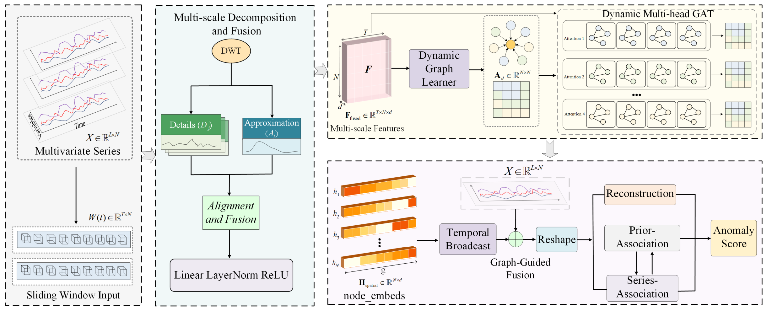
The overall data processing pipeline follows a hierarchical modeling paradigm that progresses from the frequency domain to the spatial domain and finally to the temporal domain, as illustrated in Figure 1.

Figure 1. Overall framework of the proposed WGF. Arrows indicate the flow of information, and different colors denote different functional modules.

The multi-scale temporal–frequency feature modeling module employs DWT to decompose the input sequence into low-frequency approximation coefficients and high-frequency detail coefficients. These components are aligned and fused via learnable projection layers to obtain a unified multi-scale representation. The dynamic graph learning module constructs an adaptive adjacency matrix from the fused features to capture time-varying dependencies among variables. A graph attention mechanism is then applied to perform spatial feature aggregation and learn dynamic inter-variable relationships. Based on this, a graph-guided feature modulation mechanism injects spatially enhanced graph embeddings into the temporal representation space via feature-wise affine transformation, enabling adaptive modulation of temporal features. Finally, the modulated features are projected to the target dimension and fed into the anomaly detection backbone, where anomaly scores are computed based on reconstruction error and association discrepancy.

3.3. Multi-Scale Time-Series Feature Extraction Based on Discrete Wavelet Transform

Industrial sensor data typically exhibit multi-scale superimposed patterns in the temporal domain. Long-term system evolution often forms stable trend components, while periodic fluctuations reflect production cycles and shift patterns. In addition, the data are usually contaminated with random noise and sudden perturbations. Directly feeding raw sequences into deep models may lead to interference from high-frequency noise, which can distort the inference of graph structures. In particular, in dynamic graph learning, noise may obscure the true association strengths between variables, causing spurious correlations to be mistakenly regarded as structural priors.

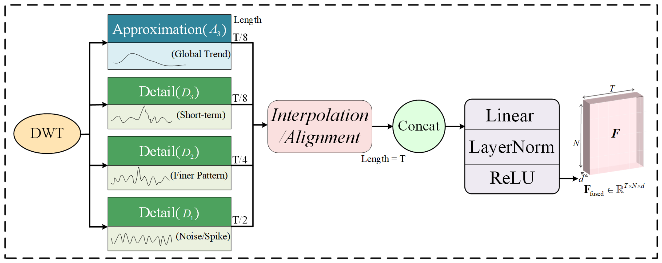
To address this issue and accurately capture patterns at different frequency components, this paper introduces the DWT as a feature decoupling operator, as illustrated in Figure 2. Given an input window $W(t)$ and a DWT operator $D(\cdot )$, the signal can be decomposed at scale j into approximation coefficients $A_j$, representing low-frequency trends, and detail coefficients $D_j$, representing high-frequency variations, thereby enabling multi-resolution temporal feature extraction.

Figure 2. Detailed architecture of the multi-scale decomposition and fusion module. Arrows indicate the flow of information.

Specifically, for the original signal $x\in {ℝ}^{T\times N}$, the DWT decomposition can be formally defined as follows:

$$\begin{array}{l}{A}_j[k]={\displaystyle \sum _{n}h}[n]\cdot A_{j-1}[2k-n],\hfill \\ D_j[k]={\displaystyle \sum _{n}g}[n]\cdot A_{j-1}[2k-n]\hfill \end{array}$$

(1)

Let h and g denote the low-pass and high-pass filters, respectively, and $j=1, 2, 3$ indicate the decomposition level, with $A_0=x$ representing the original input. The original signal undergoes a three-level decomposition to produce sub-band signals spanning different frequency ranges. In this hierarchy, $A_3$ captures the low-frequency trend component, while, $D_1, D_2$ and $D_3$ capture high-frequency detail components at progressively coarser scales.

This multi-scale decomposition achieves an implicit separation between the underlying signal and noise. By isolating the low-frequency component, the model constructs robust spatiotemporal dependencies based on purified trend information, effectively mitigating interference from high-frequency noise during graph structure inference. Concurrently, preserving the high-frequency components ensures the model retains sensitivity to transient anomalies.

Following coefficient extraction, feature refinement is applied at each scale. The coefficient sequence at each level undergoes LayerNorm to correct for amplitude-related biases. Subsequently, a learnable linear projection layer maps the normalized coefficients into a unified feature space:

$${\tilde{F}}_j=\mathrm{ReLU}\left(W_j\cdot \mathrm{LayerNorm}(C_j)+b_j\right)$$

(2)

where $C_j\in \{A_j,D_j\}$ denotes the coefficient matrix at the j-th level, $W_j$ and $b_j$ are learnable parameters, and ${\tilde{F}}_j$ represents the refined feature at the corresponding scale. To resolve sequence length inconsistencies across scales, an adaptive alignment algorithm based on linear interpolation is employed, ensuring that all feature sequences conform to the model’s preset window length T. Specifically, sequences shorter than T are upsampled via linear interpolation, whereas sequences exceeding T are downsampled accordingly.

We introduce a multi-scale feature fusion mechanism based on concatenation and linear projection. Unlike simple weighted summation, this approach concatenates all four scale features—specifically, one approximation coefficient ${\tilde{F}}_A$ and three detail coefficients ${\tilde{F}}_{D_1}, {\tilde{F}}_{D_2}, {\tilde{F}}_{D_3}$—along the feature dimension before fusing them through a dedicated linear layer:

$$F_{\mathrm{fused}}=W_f\cdot \mathrm{Concat}({\tilde{F}}_A,{\tilde{F}}_{D_1},{\tilde{F}}_{D_2},{\tilde{F}}_{D_3})+b_f$$

(3)

Here, $\mathrm{Concat}(\cdot )$ denotes the concatenation operation, and $W_f$ is a learnable fusion matrix that projects the high-dimensional concatenated features back to the target dimension d. The resultant fused feature $F_{\mathrm{fused}}$ is subsequently processed through LayerNorm and a non-linear activation function.

This design enables the model to adaptively integrate information from each scale through learnable fusion weights. The generated multi-scale feature matrix $F_{\mathrm{fused}}$, which contains rich time-frequency domain information, serves as the input for the subsequent dynamic graph structure learning module. These features preserve the temporal patterns of the original sequence, with their discriminative power enhanced via multi-scale analysis, thereby providing a more robust and information-rich representational foundation for dynamic graph structure learning.

3.4. Dynamic Graph Structure Learning

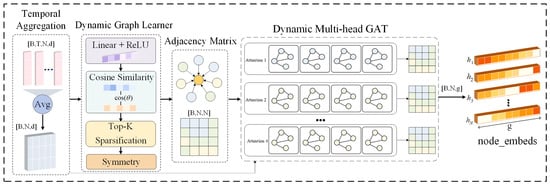
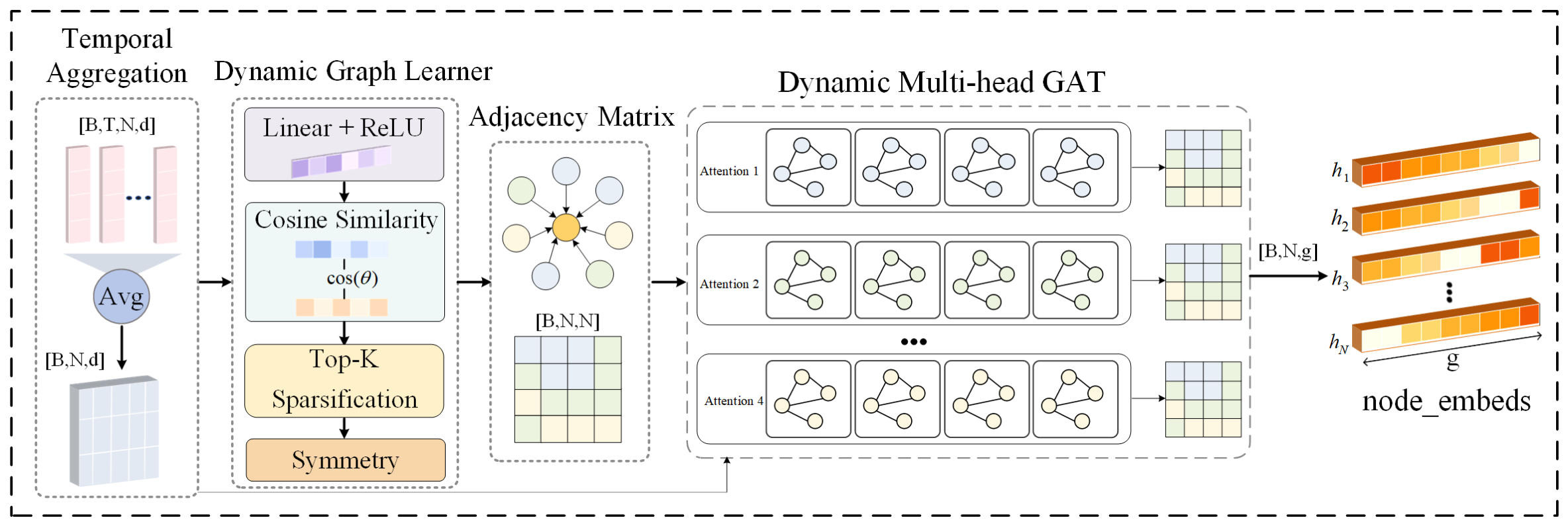
Inter-variable interactions in multivariate time series evolve dynamically with system states, exhibiting non-stationary and time-varying dependency characteristics. Traditional graph neural networks relying on static adjacency matrices struggle to adapt to such evolving patterns, while manually defined graph structures often depend heavily on domain priors and lack scalability. To address this challenge, the proposed methodology consists of three key steps, as illustrated in Figure 3: (1) temporal aggregation is first applied to obtain stable node representations; (2) a dynamic adjacency matrix construction module is then employed to infer time-varying graph structures based on feature similarity; and (3) a prior-guided multi-head graph attention network performs spatial feature encoding by leveraging the learned topology as a structural prior. Through the synergy of these steps, the model effectively captures non-stationary spatio-temporal dependencies without introducing significant computational overhead.

Figure 3. Architecture of the dynamic graph feature learning module. Arrows indicate the flow of information, and different colors denote different functional modules.

3.4.1. Dynamic Adjacency Matrix Construction

To capture time-evolving association patterns among variables, a lightweight dynamic graph construction strategy is designed. Given the multi-scale fused features $F_{\mathrm{fused}}\in {ℝ}^{T\times N\times d}$, a dynamic adjacency matrix $A_d\in {ℝ}^{N\times N}$ is constructed as follows, where each element $a_{ij}$ is constrained within $\left[0,1\right]$, representing the normalized association strength between variables i and j at the current time step.

Stable and robust node representations are obtained via a temporal aggregation operation, implemented as mean pooling over the most recent $w$ time steps, to enhance temporal stability, i.e.,

$$H^{(0)}={\displaystyle \frac{1}{w}}{\displaystyle \sum _{\tau =t-w+1}^t{F}_{\tau }^{\mathrm{fused}}}\in {ℝ}^{N\times d}$$

(4)

Which smooths short-term fluctuations and emphasizes the current behavioral patterns.

Subsequently, the aggregated features are projected into a lower-dimensional latent space to suppress noise and reduce computational overhead, yielding

$$H^{(1)}=\mathrm{ReLU}(H^{(0)}{W}_p+b_p)\in {ℝ}^{N\times d_r}$$

(5)

where $W_p\in {ℝ}^{d\times d_r}$ is a learnable projection matrix and $d_r$ denotes the latent dimensionality. The resulting representations are further normalized via ${\mathcal{l}}_2$-normalization to ensure scale consistency.

Cosine similarity is employed to measure the structural dependencies between variables, formulated as

$$S_{ij}={\displaystyle \frac{{\left(H_i^{(1)}\right)}^{\top }{H}_j^{(1)}}{\Vert H_i^{(1)}\Vert \Vert H_j^{(1)}\Vert }}$$

(6)

To obtain a sparse and generalizable graph structure, Top-$k$ sparsification is applied to retain only the most relevant neighbors for each node, followed by a symmetrization operation to enforce the undirected property, i.e.,

$$A_d={\displaystyle \frac{\widehat{S}+{\widehat{S}}^{\top }}{2}}, \mathrm{where} \widehat{S}=\mathrm{Top}-\mathrm{k}(S)$$

(7)

3.4.2. Dynamic Graph Attention Network

Guided by the dynamic adjacency matrix $A_d$, a Dynamic Graph Attention Network is employed to further model the spatial dependencies among variables. Unlike conventional Transformer-based attention, which relies solely on content features, the proposed method incorporates the dynamic graph as an explicit structural prior into the attention computation, thereby enhancing the model’s sensitivity to underlying physical dependency patterns.

For an arbitrary node pair $\left(i,j\right)$, the raw attention energy is computed based on concatenated linear projections, i.e.,

$$e_{ij}=\mathrm{LeakyReLU}\left(a^{\top }\cdot \left[W_q{h}_i\oplus W_k{h}_j\right]\right)$$

(8)

where $h_i$ and $h_j$ denote the feature representations of nodes i and j, respectively, $W_q$ and $W_k$ are learnable projection matrices, and $\oplus$ denotes the concatenation operation.

To effectively fuse data-driven attention with the structural prior, a learnable gating coefficient $\alpha \in \left[0,1\right]$, obtained via a Sigmoid mapping, is introduced to balance their contributions. Meanwhile, the dynamic adjacency value $A_d(i,j)$ is amplified to strengthen its guiding role. The refined attention score is defined as

$${\widehat{e}}_{ij}=\alpha \cdot e_{ij}+(1-\alpha )\cdot (\zeta \cdot A_d(i,j)), \zeta =\mathrm{Softplus}({\zeta }_{\mathrm{raw}}), {\zeta }_{\mathrm{raw}}\in ℝ$$

(9)

where $\zeta$ is a learnable scaling factor for the adjacency strength, constrained to be positive via the Softplus activation.

Softmax normalization is applied only to edges satisfying $A_d[i,j]>0.1$, filtering weak connections and suppressing noise propagation. The normalized attention weights are computed as

$$a_{ij}={\displaystyle \frac{\exp ({\widehat{e}}_{ij})}{{\displaystyle \sum _{k:A_d(i,k)>0.1}\exp }({\widehat{e}}_{ik})}}$$

(10)

The node representations are updated via attention-based aggregation over the selected neighbors, yielding

$${h^{\prime }}_i={\displaystyle \sum _{j:A_d(i,j)>0.1}{a}_{ij}}\cdot W_v{h}_j$$

(11)

Through this process, the local structural dependencies among variables are preserved, while enabling the model to learn more discriminative representations from global spatiotemporal interactions.

3.4.3. Prior-Guided Multi-Head Graph Attention Aggregation

To enhance the representational capacity of node features, a multi-head attention mechanism is adopted, where four parallel attention heads capture inter-node dependencies from diverse perspectives. Each head independently computes attention scores, and the resulting representations are concatenated along the feature dimension, followed by an output aggregation layer to produce unified node embeddings.

Notably, the learned attention scores are fused with the dynamic adjacency matrix as a structural prior, enabling a principled integration of data-driven and prior knowledge. A learnable weighting coefficient $\alpha \in \left[0,1\right]$, obtained via a Sigmoid mapping, is introduced to adaptively balance their contributions, i.e.,

$$e_{ij}^{fused}=\alpha \cdot e_{ij}^{learned}+(1-\alpha )\cdot e_{ij}^{prior}$$

(12)

where $e_{ij}^{prior}$ is derived from the adjacency matrix generated by the lightweight graph learner.

Through this prior-guided aggregation mechanism, the model preserves stable structural priors while maintaining the flexibility to adapt to data-driven patterns. The final node embeddings $H_{\mathrm{spatial}}\in {ℝ}^{N\times d}$ are then used as inputs to the subsequent graph-guided feature modulation module.

3.5. Spatio-Temporal-Frequency Collaborative Modeling

In the preceding modules, multi-scale frequency information is first extracted via DWT and further incorporated into dynamic graph learning, resulting in spatial representations enriched with frequency-aware priors. Meanwhile, temporal dependencies are modeled by the Transformer. To enable unified modeling across temporal, spatial, and frequency domains, this section further injects the frequency-enhanced dynamic graph as a modulation signal into the temporal modeling process.

A straightforward approach is to concatenate node embeddings with the original temporal features followed by a linear projection. However, this strategy suffers from two limitations: it leads to feature dimensionality expansion, and the graph information is merely treated as an additional channel, preventing the model from adaptively controlling the strength and direction of the structural prior. To address these issues, inspired by the Feature-wise Linear Modulation (FiLM) mechanism and the gating strategy in SE-Net, a graph-guided residual modulation scheme is proposed, which performs a feature-wise affine transformation to enable adaptive integration of structural priors into temporal representations.

Given the input $x\in {ℝ}^{T\times N\times d_{\mathrm{model}}}$ and the graph embeddings $H_{\mathrm{spatial}}\in {ℝ}^{N\times d_{\mathrm{spatial}}}$, the graph embeddings are first broadcast along the temporal dimension to align with the input sequence length. A gating network is then employed to predict modulation parameters, i.e.,

$$[\gamma ,\beta ]=\mathrm{MLP}\left(\mathrm{Broadcast}\left(H_{\mathrm{spatial}},T\right)\right)$$

(13)

where $\gamma =\sigma ({\mathrm{MLP}}_{\mathrm{scale}}(\cdot ))\in {ℝ}^{T\times N\times d_{\mathrm{model}}}$ serves as the scaling factor constrained by a Sigmoid activation, and $\beta ={\mathrm{MLP}}_{\mathrm{shift}}(\cdot )\in {ℝ}^{T\times N\times d_{\mathrm{model}}}$ denotes the unconstrained shifting term.

The modulation is implemented via a residual scaling–shifting transformation, yielding

$$X_{\mathrm{modulated}}=X_{\mathrm{raw}}\odot (1+\gamma )+\beta$$

(14)

where the scaling term is bounded within $\left(0,1\right)$ and the shifting term remains unconstrained. This formulation preserves the original features through a residual structure while enabling adaptive modulation. When the structural prior is uninformative, the learned scaling factor tends to suppress its influence, and the transformation degenerates to an identity mapping.

Finally, the modulated features are projected to the target dimension and normalized as

$$X_{\mathrm{final}}=\mathrm{LayerNorm}\left(W_{\mathrm{proj}}\cdot X_{\mathrm{modulated}}+b_{\mathrm{proj}}\right)$$

(15)

where $W_{\mathrm{proj}}\in {ℝ}^{d_{\mathrm{spatial}}\times d_{\mathrm{model}}}$. The resulting representations are then fed into the anomaly detection backbone to perform temporal dependency reconstruction and anomaly scoring.

From a modeling perspective, the proposed modulation mechanism enables the effective injection of spatial structural information into temporal representations and establishes a collaborative interaction among frequency features, spatial dependencies, and temporal modeling. Specifically, multi-scale frequency features enhance the stability and discriminative capability of graph structure learning, the dynamic graph captures time-varying inter-variable dependencies, and the modulation mechanism feeds the learned structural information back into the temporal representation space, thereby forming a closed-loop spatio-temporal-frequency collaborative modeling framework.

The key advantages of this design are as follows: graph embeddings are utilized as control signals rather than additional feature channels, introducing no extra dimensional overhead; the residual structure preserves the integrity of the original temporal information; moreover, the modulation is functionally equivalent to applying a graph-conditioned affine transformation to each variable’s representation space, enabling the dynamic graph structure to adaptively scale and shift temporal features and thus achieving deep injection of structural priors before feeding into the anomaly detection backbone.

3.6. Anomaly Detection via Association Discrepancy and Reconstruction Error

After graph-guided feature modulation, the refined representations $X_{\mathrm{final}}\in {ℝ}^{T\times N\times d_{\mathrm{model}}}$ are fed into an anomaly detection backbone following the Anomaly Transformer paradigm. In addition to association discrepancy, reconstruction error is incorporated as a complementary signal to enhance anomaly detection robustness.

Specifically, two types of temporal associations are constructed, including data-driven series attention and structure-aware prior attention. The series attention captures temporal dependencies via Query–Key projections under a causal constraint, i.e.,

$$Q=X_{\mathrm{final}}{W}_q,K=X_{\mathrm{final}}{W}_k$$

(16)

$$S^{\mathrm{attn}}=\mathrm{Softmaxrow}\left({\displaystyle \frac{Q{K}^{\top }}{\sqrt{d_k}}}\right)\circ M_{\mathrm{mask}}$$

(17)

In parallel, a Gaussian kernel is adopted to construct the prior attention $P^{\mathrm{attn}}$, whose scale parameter is dynamically predicted from the input features, enabling adaptive control of the attention decay. The discrepancy between series attention and prior attention is quantified using bidirectional Kullback–Leibler divergence:

$${\mathcal{L}}_{\mathrm{assoc}}=D_{\mathrm{KL}}\left(S^{\mathrm{attn}}\Vert P^{\mathrm{attn}}\right)+D_{\mathrm{KL}}\left(P^{\mathrm{attn}}\Vert S^{\mathrm{attn}}\right)$$

(18)

A reconstruction objective is introduced to model value-level consistency between the input and reconstructed sequences:

$$\widehat{X}=X_{\mathrm{final}}{W}_o, {\mathcal{L}}_{\mathrm{recon}}=\Vert X_{\mathrm{final}}-\widehat{X}{\Vert }_2^2$$

(19)

The model is trained via an alternating optimization strategy, which encourages the series attention to align with the prior while allowing the prior to adapt to data-driven patterns, thereby improving stability.

During inference, reconstruction errors and association discrepancies are normalized using global min–max normalization:

$${\tilde{r}}_t={\displaystyle \frac{r_t-r_{\min }}{r_{\max }-r_{\min }+ϵ}}, {\tilde{a}}_t={\displaystyle \frac{a_t-a_{\min }}{a_{\max }-a_{\min }+ϵ}}$$

(20)

The final anomaly score is computed by combining the two signals:

$${\mathrm{Score}}_t={\tilde{r}}_t\cdot (1+(1-{\tilde{a}}_t))$$

(21)

A quantile-based threshold is estimated from the training set:

$$\delta =\mathrm{Quantile}(\{{\mathrm{Score}}^{\mathrm{train}}\},1-q)$$

(22)

The prediction is given by ${\widehat{y}}_t=\mathbb{I}\left({\mathrm{Score}}_t>\delta \right)$, followed by a simple post-processing step to reduce isolated false positives.

4. Experiments and Results

4.1. Datasets

Experiments are conducted on five representative public multivariate time series datasets, including SWaT [36], WADI [37], SMAP [38], MSL [38], and SMD [10]. These datasets cover a variety of typical application scenarios, including industrial control systems (SWaT and WADI), spacecraft telemetry (SMAP and MSL), and server monitoring (SMD). They exhibit significant differences in scale, variable dimensionality, and anomaly distribution, enabling a comprehensive evaluation of model performance under diverse and complex conditions. Table 2 summarizes the detailed statistics of these datasets, including the numbers of training and testing samples, feature dimensionality, and anomaly ratios.

Table 2. Dataset information.

Dataset	Train	Test	Dimensions	Anomalies (%)
SWaT	39,600	449,919	51	11.98
WADI	627,657	172,803	127	5.99
SMAP	135,183	427,617	25	13.13
SMD	708,405	708,402	38	4.16
MSL	58,317	73,729	55	10.72

SWaT (Secure Water Treatment) is a large-scale industrial dataset collected from a water treatment testbed, containing 51 sensor and actuator signals over 11 days of continuous operation. The dataset includes various attack scenarios such as sensor manipulation and physical tampering.

WADI extends SWaT to a more complex water distribution system with 127 monitored variables. It features lower anomaly frequency and longer anomaly duration, posing additional challenges for detection sensitivity.

SMAP and MSL are spacecraft telemetry datasets from NASA missions, containing 25 and 55 channels, respectively. Anomalies are labeled based on Incident Surprise Anomaly reports, reflecting failure patterns under extreme environments.

SMD consists of five weeks of server monitoring data, including 38 system metrics such as CPU, memory, and network usage, representing real-world distributed system behavior.

4.2. Experimental Setup

All datasets are normalized using Z-score normalization and segmented into sliding windows of length 100. Precision (P), Recall (R), and F1-score (F1) are adopted as evaluation metrics, and the Area Under the ROC Curve (AUC) is additionally used to evaluate detection performance from a threshold-independent perspective:

$$P={\displaystyle \frac{\mathrm{TP}}{\mathrm{TP}+\mathrm{FP}}}$$

(23)

$$R={\displaystyle \frac{\mathrm{TP}}{\mathrm{TP}+\mathrm{TN}}}$$

(24)

$$F_1={\displaystyle \frac{2\times P\times R}{P+R}}$$

(25)

where TP, TN, FP, and FN denote true positives, true negatives, false positives, and false negatives, respectively. The ROC curve plots the true positive rate (TPR) against the false positive rate (FPR) under varying decision thresholds, and the corresponding AUC value reflects the overall discriminative capability of the model.

To evaluate detection performance on continuous anomaly segments, the Point Adjustment strategy is adopted. Under this protocol, an anomalous segment is considered correctly detected if at least one point within the segment is identified as anomalous.

The proposed model is implemented in Python 3.9 and PyTorch 2.4 with CUDA 11.2. All experiments were conducted on a workstation equipped with an NVIDIA GeForce RTX 3090 GPU, an Intel Xeon CPU, and 128 GB RAM. The Adam optimizer is used for parameter optimization, and early stopping is applied during training. For all benchmark datasets, ground-truth anomaly labels provided by the original dataset publishers are used solely for evaluation and are not involved in model training, following the standard unsupervised anomaly detection setting. The number of training epochs is set to no more than 20, depending on the convergence behavior of each dataset. The Transformer encoder is configured with a model dimension $d_{model}$ of 128, 8 attention heads, and 3 layers, while the feed-forward network dimension $d_{ff}$ is set to 512. For dynamic graph learning, Top-k sparsification is adopted with k = 10. The multi-scale feature extraction module is based on the DWT, using the db4 wavelet with a decomposition level of 3.

4.3. Baseline

To comprehensively evaluate the effectiveness of the proposed framework, we compare it with 11 representative methods covering major research paradigms, including sequence reconstruction, probabilistic modeling, adversarial learning, attention mechanisms, and graph-based approaches. Classical methods such as LSTM and LSTM-VAE [39], along with seminal models including OmniAnomaly and DAGMM [40], are adopted to assess the capability of modeling stochastic dependencies and distributional characteristics. In addition, attention-based and adversarial methods such as BeatGAN [41], TranAD, and DTAAD [42] are included, with particular emphasis on Anomaly Transformer due to its association discrepancy mechanism, which is most closely related to our approach. To further evaluate the modeling of inter-variable dependencies, graph-based methods such as MST-GAT [43] and LGAT [44] are incorporated. Moreover, TimesNet, representing state-of-the-art temporal modeling, is used as a strong reference baseline. These methods collectively ensure a comprehensive and rigorous evaluation across methodological diversity and application scenarios.

4.4. Comparison Results

The proposed method achieves consistently strong performance across five public multivariate time series anomaly detection datasets, as shown in Table 3. It outperforms existing methods with improvements ranging from 1.5% to 26.8% across different datasets. In particular, it achieves state-of-the-art F1 scores of 96.50% on SWaT, 96.49% on WADI, and 96.69% on SMAP, demonstrating strong generalization capability under diverse data characteristics.

Table 3. Performance comparison of WGF with baseline methods on multiple benchmark datasets. P, R, and F1 are reported. The best results are highlighted in bold, while the second-best results are underlined.

Method	SWaT			WADI			SMAP			MSL			SMD
	P	R	F1	P	R	F1	P	R	F1	P	R	F1	P	R	F1
LSTM	86.15	83.27	84.69	86.50	83.00	84.71	89.41	78.13	83.39	82.45	78.95	80.41	78.55	85.28	81.78
OmniAnomaly	31.58	65.41	42.63	97.82	69.57	81.31	81.30	94.19	84.34	78.48	99.24	87.65	75.81	72.61	75.44
LSTM-VAE	86.00	92.50	88.20	72.35	81.20	75.86	92.20	67.75	78.10	70.59	92.31	80.03	85.92	78.21	81.88
DAGMM	89.92	57.84	70.40	81.39	60.09	69.04	58.45	90.98	71.05	49.11	55.62	52.16	67.30	49.98	57.15
BeatGan	64.01	87.46	73.92	68.50	85.25	75.90	92.38	55.85	69.61	85.94	79.49	82.34	72.95	84.29	78.10
TranAD	97.31	68.99	81.06	40.24	83.45	54.12	80.43	99.99	89.15	72.94	32.05	43.13	68.42	79.96	73.27
DTAAD	96.97	69.57	84.62	90.17	39.10	69.50	80.43	98.91	89.45	87.67	89.99	88.32	80.25	99.98	89.63
A.T.	84.55	96.73	90.07	48.44	78.82	62.33	92.13	99.40	95.58	83.90	86.45	85.06	85.03	82.96	83.64
MST-GAT	98.73	72.41	83.55	98.24	43.51	60.31	91.26	89.83	90.04	85.06	89.20	87.68	89.51	46.49	68.74
LGAT	93.28	99.92	96.43	94.13	97.06	95.47	94.60	92.04	93.38	85.08	90.13	87.26	88.27	85.91	87.08
TimesNet	89.49	94.07	91.20	57.24	54.01	56.82	81.22	99.99	89.63	79.89	96.82	84.95	83.22	87.63	84.16
WGF	93.24	99.05	96.50	93.26	99.97	96.49	92.08	99.36	96.69	89.83	86.93	88.35	79.31	91.37	84.92

A closer analysis reveals that existing methods often exhibit dataset-dependent limitations. For instance, LGAT performs well on strongly coupled datasets such as SWaT and WADI but degrades on weakly correlated datasets, indicating limited generalization when spatial dependencies are weak. Similarly, DTAAD achieves strong results on MSL and SMD but shows noticeable degradation on the high-dimensional WADI dataset, suggesting challenges in modeling complex feature interactions. Anomaly Transformer also exhibits performance degradation on WADI, indicating sensitivity to non-stationary noise.

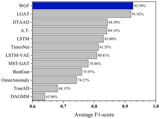
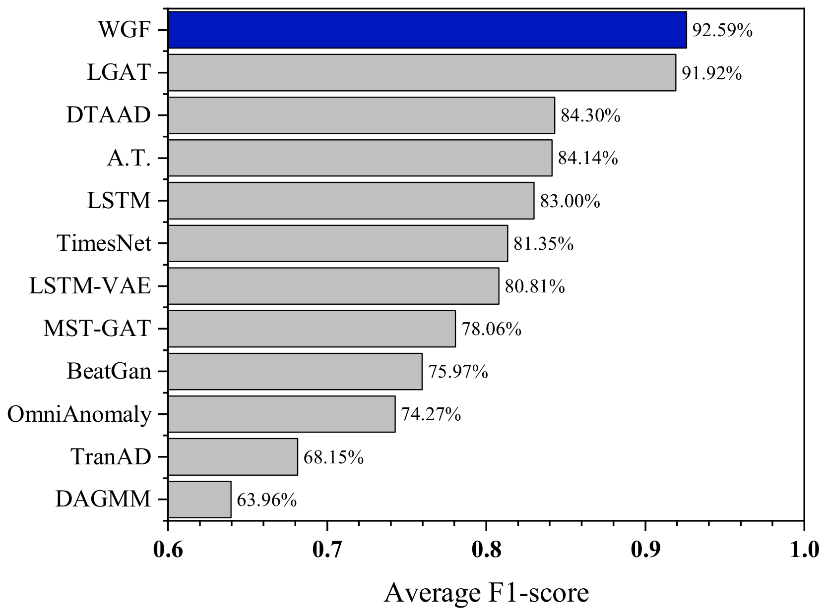
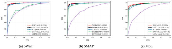
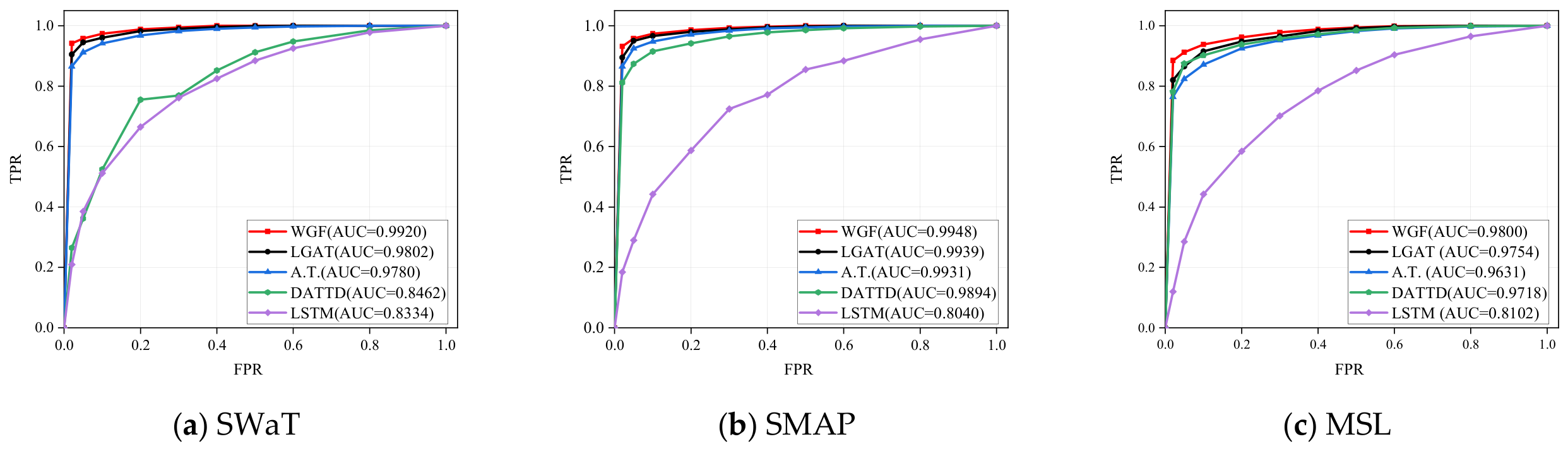
To provide an overall comparison, Figure 4 shows the average F1-score of all methods across the five datasets. The proposed method achieves the highest average F1-score, indicating more consistent performance across different scenarios compared with baseline methods. To further evaluate the detection performance from a threshold-independent perspective, Figure 5 presents the ROC curves of different models on three representative datasets.

Figure 4. Average F1-score comparison of all methods across five benchmark datasets. Blue indicates WGF; grey indicates other methods.

Figure 5. ROC curves of different models on three benchmark datasets: (a) SWaT, (b) SMAP, and (c) MSL.

It can be observed that the proposed method consistently achieves higher AUC values, indicating superior capability in distinguishing anomalies from normal patterns. These results also demonstrate that the proposed method maintains stable performance across all datasets, with F1 consistently ranging from 84.92% to 96.69%, without significant fluctuations. The consistent superiority of WGF over existing methods can be attributed to its ability to jointly model evolving spatial dependencies and multi-scale temporal patterns. Unlike graph-based baselines such as LGAT and MST-GAT, which rely on static or predefined topologies, WGF employs a dynamic sparse graph learner to capture time-varying inter-variable relationships. This capability is particularly beneficial in industrial systems where operating conditions change over time, causing sensor correlations to evolve. By adaptively updating the graph structure, WGF can better characterize dependency variations and maintain sensitivity to structural anomalies.

Another important factor is the incorporation of Discrete Wavelet Transform (DWT), which explicitly decomposes input signals into multiple frequency components before temporal modeling. Compared with methods that directly process raw time series, this design separates long-term trends from short-term fluctuations and reduces interference among mixed-frequency patterns. Consequently, the temporal encoder can focus on more informative representations, contributing to the performance gains observed across multiple datasets.

The performance advantage is further strengthened by the dual-criterion detection strategy. While conventional reconstruction-based methods primarily rely on numerical residuals, WGF jointly evaluates reconstruction error and association discrepancy. This enables the model to capture not only value-level abnormalities but also changes in dependency structures that may occur without prominent numerical deviations. The combination of multi-scale decomposition, dynamic graph learning, and structural-aware anomaly detection provides a more comprehensive characterization of anomalous behaviors, resulting in a better balance between precision and recall across different industrial scenarios.

Although the proposed method shows slightly lower performance than DTAAD on datasets with strong quasi-periodicity and weak coupling (e.g., MSL and SMD), this trade-off suggests that the model is more tailored to capturing non-stationary dynamics and complex spatio-temporal dependencies. This property may explain its strong performance on challenging datasets such as WADI, which involve high dimensionality and complex topology. Overall, the results suggest that the proposed framework achieves a good balance between robustness and adaptability across diverse scenarios.

4.5. Ablation Study

To comprehensively evaluate the contribution of each core component, ablation experiments are conducted on three representative datasets, namely SWaT, SMAP, and MSL, as summarized in Table 4. These datasets are selected due to their distinct characteristics in terms of coupling strength and temporal patterns: SWaT represents a strongly coupled industrial control system, SMAP contains pronounced non-stationary and impulsive anomalies, while MSL corresponds to relatively stable and weakly coupled spacecraft telemetry data. This combination enables a comprehensive evaluation of the proposed modules from both structural dependency and temporal complexity perspectives. Specifically, three variants are considered: (1) w/o DWT, where the DWT module is replaced with standard convolution; (2) w/o Dynamic Graph: replacing the dynamic graph learning module with a static adjacency matrix to evaluate the effectiveness of time-varying dependency modeling; and (3) w/o AT, where the Anomaly Transformer is replaced with a standard Transformer encoder, removing the association discrepancy mechanism while retaining basic temporal modeling ability, to evaluate its contribution in conjunction with the preceding modules.

Table 4. Ablation study results of WGF in terms of Precision (P), Recall (R), and F1-score (F1).

Method	SWaT			SMAP			MSL
	P(%)	R(%)	F1	P(%)	R(%)	F1	P(%)	R(%)	F1
w/o DWT	90.83	95.01	93.14	80.16	66.23	73.27	89.61	85.42	87.47
w/o Dynamic Graph	89.16	93.13	90.19	90.19	55.89	69.02	89.74	86.83	88.31
w/o AT	87.65	96.80	93.94	76.77	86.57	81.38	88.47	86.06	87.26
WGF	93.24	99.05	96.50	92.08	99.36	96.69	89.83	86.93	88.35

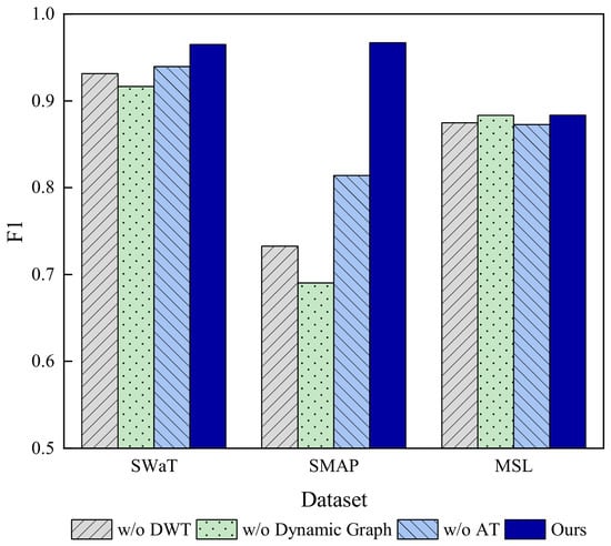
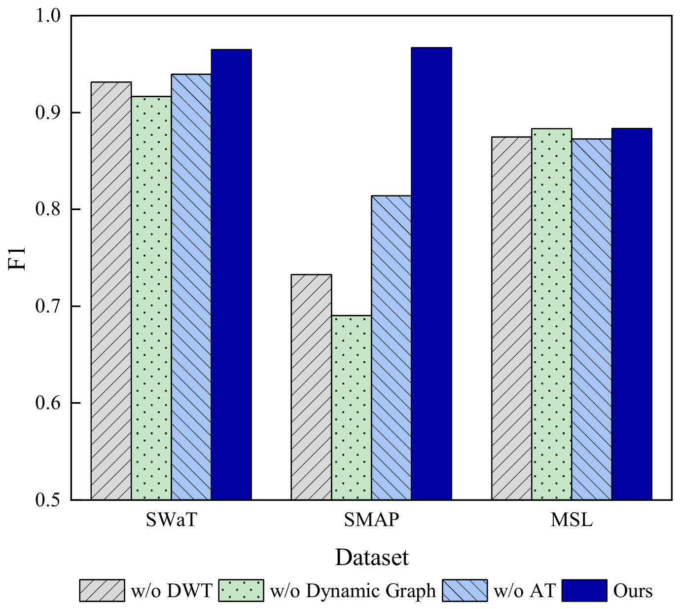
To provide a more intuitive comparison of the contribution of each component, the corresponding F1-score results are further visualized in Figure 6. As illustrated in the figure, the complete WGF model consistently achieves the highest performance across all datasets, while the removal of any individual component leads to varying degrees of performance degradation. This visual comparison further highlights the effectiveness of each module and their complementary roles within the proposed framework.

Figure 6. F1 scores of the ablation study on the SWaT, SMAP, and MSL datasets.

As shown in Table 4 and Figure 6, removing any component consistently degrades performance, confirming the effectiveness and complementarity of the proposed modules. Notably, the degree of performance degradation varies across datasets. On the SWaT dataset, removing either the DWT or dynamic graph module leads to a substantial drop in F1, whereas on the MSL dataset, the performance decline is relatively limited and remains close to that of the full model. This discrepancy can be explained by the intrinsic characteristics of the datasets. SWaT represents a strongly coupled industrial system with complex and time-varying inter-variable dependencies, making it highly reliant on both multi-scale frequency modeling and dynamic graph learning. In contrast, MSL exhibits weaker inter-variable correlations and a more stable structure, where the contribution of dynamic dependency modeling is less pronounced. Furthermore, the DWT module enhances the detection of non-stationary anomalies by disentangling frequency components, while the Anomaly Transformer provides essential global temporal modeling through the association discrepancy mechanism.

These observations validate the design rationale of the proposed framework from a collaborative modeling perspective. Specifically, multi-scale time–frequency modeling improves the discriminability of complex anomaly patterns, dynamic graph learning captures time-varying inter-variable dependencies, and the graph-guided feature modulation mechanism injects structural information into temporal representations. The synergy among these components enables effective interaction across frequency, spatial, and temporal domains, which is the key factor underlying the model’s robust and stable performance across diverse datasets.

4.6. Parameter Sensitivity Analysis

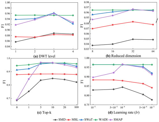
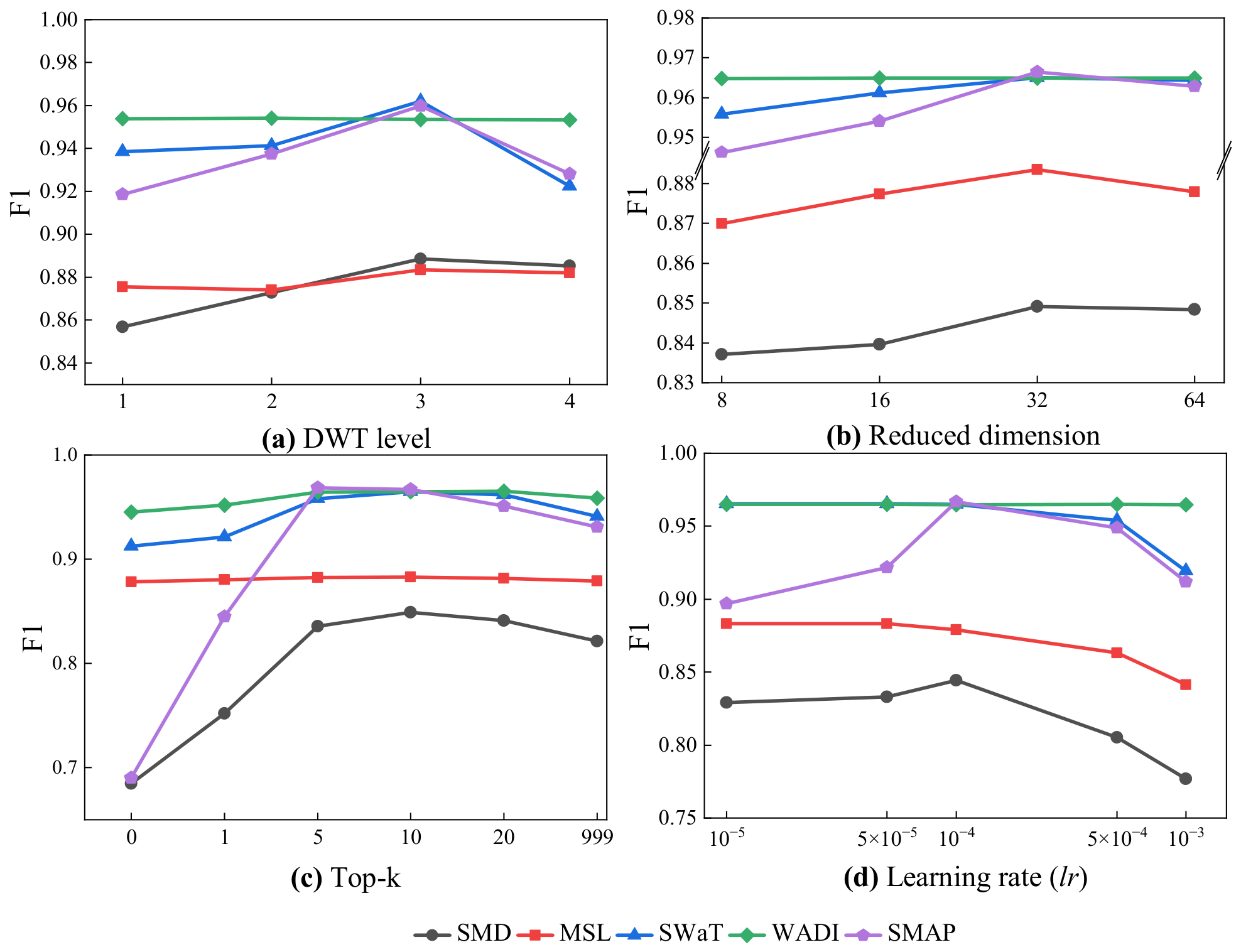
To systematically evaluate the impact of key hyperparameters on anomaly detection performance, sensitivity analyses are conducted on four representative datasets with respect to the DWT decomposition level, reduced dimension in the graph learner, Top-k sparsification, and learning rate. These parameters are closely aligned with the core components of the proposed framework: the DWT level controls the granularity of time–frequency decomposition, the reduced dimension governs the capacity of dynamic graph representation, the Top-k parameter regulates the sparsity of spatial dependencies, and the learning rate affects the convergence and stability of the optimization process. Therefore, this analysis provides a comprehensive understanding of model robustness from the perspectives of feature extraction, structural learning, and optimization. The results are illustrated in Figure 7.

Figure 7. Sensitivity analysis of key hyperparameters on five benchmark datasets. (a) Effect of DWT decomposition levels. (b) Effect of reduced dimension size. (c) Effect of Top-k sparsification. (d) Effect of learning rate.

Regarding the DWT decomposition level, as shown in Figure 7a, the F1 score first increases and then decreases as the decomposition depth grows. Increasing the level from 1 to 3 improves performance by approximately 3–8% on SWaT and SMD, with a more pronounced gain observed on SMAP. This suggests that multi-scale decomposition may help capture non-stationary patterns. However, further increasing the level leads to performance degradation, especially on MSL, indicating that excessive decomposition introduces noise. Overall, these results show that DWT primarily enhances discriminative features by separating frequency components rather than merely denoising.

For graph-related parameters, including reduced dimensionality and Top-k sparsification, consistent trends are observed. As shown in Figure 7b, increasing the reduced dimensionality from 8 to 32 leads to performance improvements of approximately 2–6%, while larger dimensions result in marginal gains or slight degradation, reflecting a trade-off between representation capacity and generalization. Similarly, Figure 7c shows that performance peaks around k = 10, with improvements of 4–10%, and declines as k increases due to the inclusion of weak or noisy connections. These results suggest that effective graph learning requires both compact representations and appropriate sparsity to capture essential inter-variable dependencies.

Regarding the learning rate, Figure 7d shows that optimal performance is achieved around 1 × 10⁻⁴. Smaller learning rates lead to slow convergence and lower performance, while increasing the rate improves F1 scores by approximately 5–12%. However, excessively large learning rates result in unstable training and noticeable degradation. This is likely because large parameter updates disrupt the coordination between dynamic graph learning and temporal modeling. Based on these observations, an initial learning rate of 1 × 10⁻⁴ with a cosine annealing schedule is adopted to balance convergence speed and stability.

It is worth noting that the performance curves remain relatively flat around the optimal hyperparameter settings. This stability suggests that WGF is robust to minor parameter perturbations (e.g., within a ±10% range), which is a desirable property for practical deployment in complex industrial environments.

5. Discussion and Conclusions

5.1. Effectiveness Analysis

5.1.1. Necessity of Multi-Scale Time–Frequency Decomposition

Ablation results (Table 4) show that removing the DWT-based module leads to a notable drop in F1, particularly on datasets with pronounced non-stationary patterns, indicating the importance of multi-scale decomposition. Industrial sensor data typically consist of mixed frequency components, including low-frequency trends, periodic patterns, and high-frequency disturbances. Without explicit frequency separation, high-frequency noise can interfere with similarity computation and consequently degrade dependency modeling.

By decomposing signals into multiple frequency bands, DWT enables the model to capture both smooth variations and localized fluctuations. A moderate decomposition level generally provides a balance between representation capacity and statistical stability. This design improves the robustness of normal pattern modeling while enhancing sensitivity to anomalous fluctuations.

5.1.2. Effectiveness of Dynamic Graph Structure Learning

The dynamic graph learning mechanism improves performance by enabling time-varying modeling of inter-variable dependencies. Instead of relying on a fixed topology, the model constructs adjacency relationships adaptively for each time window, allowing it to better reflect evolving system states.

The effectiveness of this design is further influenced by the Top-k sparsification strategy. As observed in the parameter analysis, overly dense connections tend to introduce redundant or noisy edges, while overly sparse graphs may lose essential relational information. Selecting an appropriate sparsity level allows the model to focus on the most relevant variable interactions, improving the quality of feature aggregation and overall stability of dependency modeling.

5.1.3. Effectiveness of Graph-Guided Fusion Mechanism

Compared with direct feature concatenation, the proposed graph-guided fusion mechanism provides a more structured way to incorporate relational information. The residual modulation scheme (Equation (14)) injects graph embeddings into temporal representations as adaptive control signals, allowing the model to regulate the influence of structural information.

The behavior of this mechanism depends on the quality of the learned graph representations. When graph embeddings are weakly correlated with the current sample, the modulation tends to approximate an identity mapping, thereby limiting the impact of unreliable structural cues. In contrast, informative graph embeddings are amplified through the modulation process. This adaptive behavior improves both robustness and representational flexibility.

5.1.4. Effectiveness of the Spatio–Temporal–Frequency Collaborative Framework

The proposed framework integrates multi-scale feature extraction, dynamic graph learning, and graph-guided fusion into a unified spatio–temporal–frequency modeling paradigm. Each component contributes complementary information: multi-scale features enhance temporal representations, dynamic graphs capture time-varying dependencies, and the fusion mechanism injects structural information into temporal modeling.

In addition, the dual-criterion detection strategy, which combines association discrepancy and reconstruction error, enables the model to capture both structural deviations and numerical anomalies. This collaborative design improves robustness and generalization across diverse scenarios. These advantages are reflected in the consistent performance observed in Table 3 and the robustness illustrated in Figure 4.

5.2. Limitations and Applicability Analysis

Despite achieving strong performance across multiple industrial scenarios, the proposed method still exhibits certain limitations. The computational complexity is primarily dominated by the attention-based dynamic graph aggregation process, which scales quadratically with the number of variables. Although cosine similarity computation in dynamic graph learning is relatively efficient, the overall cost is still governed by graph attention operations, leading to significant computational and memory overhead in large-scale industrial systems with high-dimensional sensor inputs. While reducing the projection dimension can partially alleviate this issue, more efficient sparse or approximate graph learning strategies remain essential for scalable deployment.

The current framework relies on fixed-length sliding windows for temporal modeling. While this design is effective for capturing local temporal dependencies and abrupt anomalies, it is less capable of modeling long-term evolutionary patterns such as gradual equipment degradation or system drift, where long-range temporal dependencies are not fully captured.

From the perspective of applicability, the proposed method performs particularly well in industrial systems with strong physical coupling, such as SWaT and WADI, where variables exhibit stable and interpretable dependencies. In such scenarios, dynamic graph learning effectively captures evolving relational structures under varying operating conditions, leading to clear advantages over purely temporal modeling approaches. For weakly coupled datasets such as MSL and SMAP, the model can still discover latent variable relationships in a data-driven manner; however, the benefits of explicit graph modeling become less pronounced. When inter-variable dependencies are extremely weak or nearly independent, the advantage of graph-based modeling further diminishes, and alternative modeling paradigms may be more appropriate.

5.3. Conclusions and Future Work

This study presents WaveGraphFormer (WGF), a unified framework designed to address the limitations of static spatial modeling and single-scale temporal representations in multivariate time-series anomaly detection. By integrating Discrete Wavelet Transform (DWT) for multi-scale frequency decomposition, a Top-k sparse dynamic graph learner for evolving inter-variable dependencies, and a graph-guided fusion mechanism for joint spatio-temporal representation, WGF achieves a comprehensive characterization of complex industrial data. Furthermore, the adoption of a dual-criterion detection strategy enhances the model’s robustness by accounting for both numerical and structural deviations.

Experimental results on five public benchmark datasets (SWaT, WADI, SMD, MSL, and SMAP) demonstrate that WGF consistently outperforms state-of-the-art baselines. These findings underscore the effectiveness of the proposed spatio-temporal-frequency collaborative framework in capturing anomalies in highly coupled and non-stationary industrial systems.

Future work will focus on improving the computational efficiency of the dynamic graph attention mechanism to support larger-scale deployments. We also plan to investigate more sophisticated temporal architectures to capture long-term system degradation patterns. Developing adaptive graph learning mechanisms capable of automatically adjusting graph structures under different operating conditions is another important direction. Incorporating causal dependency modeling into dynamic graph construction may help distinguish structural anomalies from transient fluctuations and improve the interpretability of anomaly detection results.

References

- Liu, W.; Yan, L.; Ma, N.; Wang, G.; Ma, X.; Liu, P.; Tang, R. Unsupervised Deep Anomaly Detection for Industrial Multivariate Time Series Data. Appl. Sci. 2024, 14, 774. [Google Scholar] [CrossRef] [Scilit]
- Chen, K.; Feng, M.; Wirjanto, T.S. Multivariate Time Series Anomaly Detection via Dynamic Graph Forecasting. arXiv 2023, arXiv:2302.02051. [Google Scholar]
- Correia, L.; Goos, J.-C.; Klein, P.; Bäck, T.; Kononova, A.V. Online model-based anomaly detection in multivariate time series: Taxonomy, survey, research challenges and future directions. Eng. Appl. Artif. Intell. 2024, 138, 109323. [Google Scholar] [CrossRef] [Scilit]
- Breunig, M.M.; Kriegel, H.-P.; Ng, R.T.; Sander, J. LOF: Identifying density-based local outliers. SIGMOD Rec. 2000, 29, 93–104. [Google Scholar] [CrossRef] [Scilit]
- Schölkopf, B.; Platt, J.C.; Shawe-Taylor, J.; Smola, A.J.; Williamson, R.C. Estimating the Support of a High-Dimensional Distribution. Neural Comput. 2001, 13, 1443–1471. [Google Scholar] [CrossRef] [Scilit] [PubMed]
- Chandola, V.; Banerjee, A.; Kumar, V. Anomaly Detection: A Survey. ACM Comput. Surv. 2009, 41, 15. [Google Scholar] [CrossRef] [Scilit]
- Kant, N.; Mahajan, M. Time-Series Outlier Detection Using Enhanced K-Means in Combination with PSO Algorithm. In Engineering Vibration, Communication and Information Processing; Springer Nature: Singapore, 2019; pp. 363–373. [Google Scholar]
- Xu, D.; Wang, Y.; Meng, Y.; Zhang, Z. An improved data anomaly detection method based on isolation forest. In Proceedings of the 2017 10th International Symposium on Computational Intelligence and Design, ISCID, Hangzhou, China, 9–10 December 2017; IEEE: Piscataway, NJ, USA, 2017; Volume 2, pp. 287–291. [Google Scholar] [CrossRef] [Scilit]
- Goldstein, M.; Dengel, A. Histogram-based outlier score (hbos): A fast unsupervised anomaly detection algorithm. In Proceedings of the KI-2012: Poster and Demo Track, Berlin, Germany, 17–21 September 2012; pp. 59–63. [Google Scholar]
- Su, Y.; Zhao, Y.; Niu, C.; Liu, R.; Sun, W.; Pei, D. Robust Anomaly Detection for Multivariate Time Series through Stochastic Recurrent Neural Network. In Proceedings of the 25th ACM SIGKDD International Conference on Knowledge Discovery & Data Mining; ACM: New York, NY, USA, 2019; pp. 2828–2837. [Google Scholar]
- Du, M.; Li, F.; Zheng, G.; Srikumar, V. DeepLog: Anomaly Detection and Diagnosis from System Logs through Deep Learning. In Proceedings of the 2017 ACM SIGSAC Conference on Computer and Communications Security (CCS ’17), Dallas, TX, USA, 30 October–3 November 2017; ACM: New York, NY, USA, 2017; pp. 1285–1298. [Google Scholar] [CrossRef] [Scilit]
- Rezende, D.J.; Mohamed, S.; Wierstra, D. Stochastic Backpropagation and Approximate Inference in Deep Generative Models. In Proceedings of the 31st International Conference on Machine Learning (ICML), Beijing, China, 21–26 June 2014; PMLR: New York, NY, USA, 2014; pp. 1278–1286. [Google Scholar]
- Goodfellow, I.J.; Pouget-Abadie, J.; Mirza, M.; Xu, B.; Warde-Farley, D.; Ozair, S.; Courville, A.; Bengio, Y. Generative Adversarial Nets. In Advances in Neural Information Processing Systems 27 (NIPS 2014); Curran Associates, Inc.: Red Hook, NY, USA, 2014; pp. 2672–2680. [Google Scholar]
- Chen, X.; Kingma, D.P.; Salimans, T.; Duan, Y.; Dhariwal, P.; Schulman, J.; Sutskever, I.; Abbeel, P. Variational Lossy Autoencoder. arXiv 2017, arXiv:1611.02731. [Google Scholar]
- Deng, A.; Hooi, B. Graph Neural Network-Based Anomaly Detection in Multivariate Time Series. Proc. AAAI Conf. Artif. Intell. 2021, 35, 4027–4035. [Google Scholar] [CrossRef] [Scilit]
- Wu, Z.; Pan, S.; Chen, F.; Long, G.; Zhang, C.; Yu, P.S. A Comprehensive Survey on Graph Neural Networks. IEEE Trans. Neural Netw. Learn. Syst. 2021, 33, 4–25. [Google Scholar] [CrossRef] [Scilit] [PubMed]
- Rumelhart, D.E.; Hinton, G.E.; Williams, R.J. Learning representations by back-propagating errors. Nature 1986, 323, 533–536. [Google Scholar] [CrossRef] [Scilit]
- Hochreiter, S.; Schmidhuber, J. Long short-term memory. Neural Comput. 1997, 9, 1735–1780. [Google Scholar] [CrossRef] [Scilit] [PubMed]
- Cho, K.; Van Merriënboer, B.; Gülçehre, Ç.; Bahdanau, D.; Bougares, F.; Schwenk, H.; Bengio, Y. Learning phrase representations using RNN encoder–decoder for statistical machine translation. In Proceedings of the 2014 Conference on Empirical Methods in Natural Language Processing (EMNLP), Doha, Qatar, 25–29 October 2014; Association for Computational Linguistics: Stroudsburg, PA, USA, 2014; pp. 1724–1734. [Google Scholar]
- Xu, J.; Wu, H.; Wang, J.; Long, M. Anomaly transformer: Time series anomaly detection with association discrepancy. In Proceedings of the International Conference on Learning Representations (ICLR), Online, 25–29 April 2022. [Google Scholar] [CrossRef] [Scilit]
- Liu, J.; Xie, G.; Wang, J.; Li, S.; Wang, C.; Zheng, F.; Jin, Y. Deep industrial image anomaly detection: A survey. Mach. Intell. Res. 2024, 21, 104–135. [Google Scholar] [CrossRef] [Scilit]
- Jia, N.; Cheng, Y.; Liu, Y.; Tian, Y. Intelligent Fault Diagnosis of Rotating Machines Based on Wavelet Time-Frequency Diagram and Optimized Stacked Denoising Auto-Encoder. IEEE Sens. J. 2022, 22, 17139–17150. [Google Scholar] [CrossRef] [Scilit]
- Zheng, Y.; Wang, H.; Wei, Z.; Liu, J.; Wang, S. Instant graph neural networks for dynamic graphs. In Proceedings of the 28th ACM SIGKDD Conference on Knowledge Discovery and Data Mining; ACM: New York, NY, USA, 2022; pp. 2605–2615. [Google Scholar]
- Vaswani, A.; Shazeer, N.; Parmar, N.; Uszkoreit, J.; Jones, L.; Gomez, A.N.; Kaiser, L.; Polosukhin, I. Attention Is All You Need. In Advances in Neural Information Processing Systems 30 (NIPS 2017); Curran Associates, Inc.: Red Hook, NY, USA, 2017; pp. 5998–6008. [Google Scholar]
- Tuli, S.; Casale, G.; Jennings, N.R. TranAD: Deep Transformer Networks for Anomaly Detection in Multivariate Time Series Data. Proc. VLDB Endow. 2022, 15, 1201–1214. [Google Scholar] [CrossRef] [Scilit]
- Yang, C.; Wang, T.; Yan, X. DDMT: Denoising diffusion mask transformer models for multivariate time series anomaly detection. arXiv 2023, arXiv:2310.08800. [Google Scholar]
- Zhao, H.; Wang, Y.; Duan, J.; Huang, C.; Cao, D.; Tong, Y.; Xu, B.; Bai, J.; Tong, J.; Zhang, Q. Multivariate time-series anomaly detection via graph attention network. In Proceedings of the 2020 IEEE International Conference on Data Mining (ICDM), Sorrento, Italy, 17–20 November 2020; IEEE: Piscataway, NJ, USA, 2020; pp. 841–850. [Google Scholar]
- He, Q.; Wang, G.; Lu, S.; Chen, L. Multivariate time-series anomaly detection via temporal convolutional and graph attention networks. J. Intell. Fuzzy Syst. 2023, 44, 5375–5388. [Google Scholar] [CrossRef] [Scilit]
- Gao, R.; Wang, J.; Yu, Y.; Wu, J.; Zhang, L. Enhanced graph diffusion learning with dynamic transformer for anomaly detection in multivariate time series. Neurocomputing 2025, 619, 129168. [Google Scholar] [CrossRef] [Scilit]
- Zhao, M.; Peng, H.; Li, L.; Ren, Y. Graph attention network and informer for multivariate time series anomaly detection. Sensors 2024, 24, 1522. [Google Scholar] [CrossRef] [Scilit] [PubMed]
- Li, Z.; Zhang, H.; Zheng, W. STformer: Spatio-Temporal Transformer for Multivariate Time Series Anomaly Detection. In Artificial Neural Networks and Machine Learning—ICANN 2024; Lecture Notes in Computer Science; Springer: Cham, Switzerland, 2024; pp. 297–311. [Google Scholar] [CrossRef] [Scilit]
- Liu, J.; Li, Q.; An, S.; Ezard, B.; Li, L. EdgeConvFormer: Dynamic graph CNN and transformer based anomaly detection in multivariate time series. arXiv 2023, arXiv:2312.01729. [Google Scholar]
- Chen, Y.; Liu, S.; Yang, J.; Jing, H.; Zhao, W.; Yang, G. A Joint Time-Frequency Domain Transformer for Multivariate Time Series Forecasting. Neural Netw. 2024, 176, 106334. [Google Scholar] [CrossRef] [Scilit] [PubMed]
- Wu, H.; Hu, T.; Liu, Y.; Zhou, H.; Wang, J.; Long, M. TimesNet: Temporal 2D-Variation Modeling for General Time Series Analysis. In Proceedings of the 11th International Conference on Learning Representations (ICLR), Kigali, Rwanda, 1–5 May 2023. [Google Scholar] [CrossRef] [Scilit]
- Yang, L.; Hong, S. Unsupervised time-series representation learning with iterative bilinear temporal-spectral fusion. In Proceedings of the 39th International Conference on Machine Learning, Baltimore, MD, USA, 17–23 July 2022; PMLR: New York, NY, USA, 2022; pp. 25038–25054. [Google Scholar]
- Mathur, A.P.; Tippenhauer, N.O. SWaT: A water treatment testbed for research and training on ICS security. In Proceedings of the 2016 International Workshop on Cyber-Physical Systems for Smart Water Networks (CySWater), Singapore, 11 April 2016; pp. 31–36. [Google Scholar] [CrossRef] [Scilit]
- Ahmed, C.M.; Palleti, V.R.; Mathur, A.P. WADI: A Water Distribution Testbed for Research in the Design of Secure Cyber Physical Systems. In Proceedings of the 3rd International Workshop on Cyber-Physical Systems for Smart Water Networks (CySWATER’17), Pittsburgh, PA, USA, 21 April 2017; pp. 25–28. [Google Scholar] [CrossRef] [Scilit]
- Hundman, K.; Constantinou, V.; Laporte, C.; Colwell, I.; Soderstrom, T. Detecting spacecraft anomalies using LSTMs and nonparametric dynamic thresholding. In Proceedings of the 24th ACM SIGKDD International Conference on Knowledge Discovery & Data Mining (KDD’18), London, UK, 19–23 August 2018; pp. 387–395. [Google Scholar] [CrossRef] [Scilit]
- Lin, S.; Clark, R.; Birke, R.; Schönborn, S.; Trigoni, N.; Roberts, S. Anomaly Detection for Time Series Using VAE-LSTM Hybrid Model. In Proceedings of the IEEE International Conference on Acoustics, Speech and Signal Processing (ICASSP), Barcelona, Spain, 4–8 May 2020; pp. 4322–4326. [Google Scholar] [CrossRef] [Scilit]
- Zong, B.; Song, Q.; Min, M.R.; Cheng, W.; Lumezanu, C.; Cho, D.; Chen, H. Deep autoencoding Gaussian mixture model for unsupervised anomaly detection. In Proceedings of the International Conference on Learning Representations (ICLR), Vancouver, BC, Canada, 30 April–3 May 2018. [Google Scholar]
- Zhou, B.; Liu, S.; Hooi, B.; Cheng, X.; Ye, J. BeatGAN: Anomalous rhythm detection using adversarially generated time series. In Proceedings of the 28th International Joint Conference on Artificial Intelligence (IJCAI-19), Macao, China, 10–16 August 2019; pp. 4433–4439. [Google Scholar] [CrossRef] [Scilit] [PubMed]
- Yu, L.R.; Lu, Q.H.; Xue, Y. DTAAD: Dual TCN-attention networks for anomaly detection in multivariate time series data. Knowl.-Based Syst. 2024, 295, 111849. [Google Scholar] [CrossRef] [Scilit]
- Ding, C.; Sun, S.; Zhao, J. MST-GAT: A multimodal spatial–temporal graph attention network for time series anomaly detection. Inf. Fusion 2023, 89, 527–536. [Google Scholar] [CrossRef] [Scilit]
- Wen, M.; Chen, Z.; Xiong, Y.; Zhang, Y. LGAT: A novel model for multivariate time series anomaly detection with improved anomaly transformer and learning graph structures. Neurocomputing 2025, 617, 129024. [Google Scholar] [CrossRef] [Scilit]
Disclaimer/Publisher’s Note: The statements, opinions and data contained in all publications are solely those of the individual author(s) and contributor(s) and not of MDPI and/or the editor(s). MDPI and/or the editor(s) disclaim responsibility for any injury to people or property resulting from any ideas, methods, instructions or products referred to in the content. |
© 2026 by the authors. Licensee MDPI, Basel, Switzerland. This article is an open access article distributed under the terms and conditions of the Creative Commons Attribution (CC BY) license.