


Abstract
Quantitative evaluation of public transit networks (PTNs) with complex-network models informs route optimization and operational adjustments. Prior studies emphasize large cities and pay limited attention to small-sized urban systems. This study examines the bus network of Cangzhou City, Hebei Province, China, to broaden the empirical scope and characterize PTNs in smaller cities. The dataset for this study comprises route and stop records, passenger boarding logs, and bus GPS traces. We develop a general workflow for bus data cleaning and completion. To characterize the dynamic bus network and compare it with the static network, we construct a static network and Directed Weighted Dynamic Network I (DWDN I) using the L-space method, and we construct Directed Weighted Dynamic Network II (DWDN II) using the P-space method. We calculated network metrics including degree, weighted degree, clustering coefficient, path length, network diameter, network efficiency, and small-world coefficient. The principal results show that: (1) at the macroscopic level, the dynamic PTN tracks passenger demand, as the average degree, weighted average degree, and clustering coefficient fluctuate in concert with passenger flows; (2) key stations concentrate in the urban core, and stations with high weighted degree display pronounced spatial autocorrelation; (3) the exponential form of the weighted-degree distribution indicates that the examined bus network is not scale-free, while the dynamic network’s small-world coefficient exceeds that of the static network across time periods, reflecting stronger small-world characteristics. This study integrates network and spatial attributes of the PTN to offer an exploratory case for investigating public transit networks in third-tier cities. The findings can inform comparable studies and offer practical guidance for bus operators.
1. Introduction
Public transit, owing to its high capacity and low cost, is central to reducing urban congestion and environmental pollution [1]. In densely populated developing countries such as China, prioritizing public transportation development yields particular benefits. Research on public transit systems clarifies operational mechanisms, informs design and optimization, and ultimately improves operational efficiency [2].
Complex network theory provides a powerful framework for characterizing the topology of urban transportation networks [3]. In China, researchers have widely applied this framework to study public transit systems in first- and second-tier cities. Using core topological metrics—degree distribution, path length, and centrality—studies reveal the fundamental structural properties of urban bus networks. These metrics also enable identification of key nodes and assessment of network robustness. When combined with population distribution and POI data, the approach supports evaluations of the spatial equity of bus service [4]. Together, these findings offer theoretical guidance for optimizing bus routes and operational scheduling.
Research on PTNs in third-tier cities has received insufficient attention from the academic community. Influenced by population distribution, land use, and city size, these networks display structural features that differ from those of large cities, such as an absence of pronounced hub nodes. At the same time, residents’ travel patterns in third-tier cities are relatively limited, and buses play a more critical role in serving low-income groups and the elderly and in maintaining social equity. Existing studies have shown that developing public transit in small cities can yield higher returns on benefits [5]. Thus, studying bus networks in third-tier cities carries important theoretical and practical significance.
With advances in the informatization of public-transport infrastructure, access to multi-source big data—bus GPS trajectories, passenger boarding records, and spatial data on routes and stops—has steadily improved [6,7]. These data enable analysis of the bus network’s dynamic characteristics. Examining the spatiotemporal evolution of the PTNs using multi-source big data provides a reliable empirical basis and decision support for optimizing network layout and developing evidence-based bus operation plans.
Cangzhou is a representative third-tier Chinese city with a strategic location inside the Beijing–Tianjin–Hebei urban agglomeration. Driven by the coordinated development policy for that region, Cangzhou has undergone marked urban growth and structural transformation in recent years. In 2023, the Transport Services Department of the Ministry of Transport selected Cangzhou for a demonstration project to build a national public-transport metropolis during the 14th Five-Year Plan. Examining Cangzhou’s public-transport network therefore provides practical technical guidance for its metropolitan public-transport development and yields a representative case for studying public-transport systems in third-tier cities, thereby broadening the scope of urban public-transport network research.
Overall, research on PTNs in China and elsewhere has concentrated on large and medium-sized cities, leaving PTNs in smaller cities underexamined. Moreover, most models are static and seldom incorporate the spatiotemporal dynamics of passenger flows or the operational characteristics of buses, and also lack sufficient consideration of the spatial attributes of PTNs [8]. Studies also typically model a single PTN, which yields an incomplete representation of the system.
To address these gaps, this study analyzes the PTN of Cangzhou, a third-tier city in Hebei Province, China. We classify bus operations into peak, off-peak, and trough periods based on passenger boarding data. We then construct a static bus network and DWDN I using the L-space method and build DWDN II using the P-space method. For both dynamic networks, the bus network is split into two directional components according to dir values (0 or 1). In DWDN I, stops serve as nodes, and edge weights equal the hourly volume of passing vehicles; in DWDN II, stops serve as nodes, and edge weights equal the average bus travel time per hour. From DWDN I, we compute degree, weighted degree, and clustering coefficient, and we visualize their temporal and spatial distributions. We assess scale-free behavior by fitting the cumulative weighted-degree distribution. From DWDN II, we compute path length, network diameter, network efficiency, and three centrality indicators. Using these measures together with the clustering coefficient, we quantitatively calculate small-world network indicators.
The paper is organized as follows. Section 2 reviews international research on static and dynamic bus networks. Section 3 details methods for acquiring and processing PTN data, passenger boarding records, and bus GPS traces. Section 4 presents the three network models developed in this study and their associated indicators. Section 5 assesses the characteristics of the PTNs in Cangzhou City. Section 6 discusses the research findings. Finally, Section 7 summarizes the contributions and outlines directions for future work.
2. Related Work
Since Watts and Strogatz introduced small-world networks in 1998, complex network theory has drawn cross-disciplinary attention and has become a widely used modeling paradigm in transit studies [9]. Contemporary approaches employ three principal topological representations: L-space, P-space, and R-space [10,11]. In the L-space model, stops serve as nodes, and edges connect adjacent stops along the same route, producing a network that mirrors the physical PTN and thus is frequently used in empirical work [12]. The P-space model also treats stops as nodes, but it links any two stations that share a route regardless of adjacency, which makes P-space better suited for analyzing transfer behavior [4]. The R-space model represents bus lines as nodes and creates edges between lines when they share stations, so it is chiefly used to study bus transfers while obscuring details about individual transfer stations [10].
PTNs can be categorized into static and dynamic models according to whether temporal and spatial dynamic variables are incorporated into the modeling process. This paper reviews the research progress of static and dynamic PTN models and summarizes the deficiencies of existing research.
2.1. Static PTNs
Early studies in China primarily constructed static, city-level network models. Using the P-space method, Xu et al. [13] analyzed PTNs in 330 Chinese cities and found that the degree distribution generally followed an exponential form and that the networks exhibited small-world properties. Tang et al. [14] and Di et al. [15] applied the L-space method to bus systems in Changsha and Chengdu, respectively, and reported that both cities’ PTNs exhibited small-world and scale-free characteristics. In a later study, Cao et al. [16] constructed a directed L-space network for Changsha and found that the bus network displayed scale-free rather than small-world characteristics, a result that may reflect the strengthening of network hubs in Changsha. Zhang et al. [17] and Pu et al. [18] built a bus-network model for Lanzhou and a comprehensive public-transport network model combining rail transit and conventional buses, respectively, and reported that both static networks showed scale-free characteristics. Kong et al. [19] constructed a bus-transfer network using the P-space method and found that Beijing’s PTN displays small-world but not scale-free properties. Hu et al. [20] developed static directed L-space and P-space models for Harbin’s public-transport network, calculated node-degree and path-length metrics, and introduced a detour coefficient to quantify detour behavior. Jia et al. [21] proposed a PTN model for Xi’an and formulated a network-optimization problem, offering a solution based on betweenness centrality. Wang et al. [8] introduced a geospatial network-analysis approach that couples spatial and network analyses; using subdistrict and hexagonal grid units, they built two bus-network models for Hangzhou that exhibit both small-world and scale-free characteristics. Háznagy A et al. [22] constructed both weighted networks, using peak average passenger loads as edge weights, and unweighted networks for five medium-sized Hungarian cities. They reported that all five transportation networks exhibited small-world properties, that the unweighted networks’ degree distributions decayed exponentially, and that the weighted networks followed power-law distributions. In contrast, studies in China found that weighted and unweighted networks generally shared the same distributional characteristics. Robin et al. [23] applied the L-space method to analyze the UK’s bus, rail, and coach networks at the national scale and found that PTN node-degree distributions followed a power-law decay, indicating a scale-free structure. Bona et al. [24] introduced a Reduced Model to mitigate the analytical impact of the many nodes with degree 1 or 2 and applied it to four large PTNs. Their results showed that preserving the network skeleton emphasized a hub-centered hierarchical organization and the small-world relationships among hubs. Tran et al. [25] reported that the bus network in Hanoi displayed scale-free characteristics. Hong et al. [26] examined individual bus and subway networks and their integrated form in the Seoul Metropolitan Area, finding that none of the three networks exhibited small-world properties and that only the bus network was scale-free. Shanmukhappa et al. [27] compared the bus networks of Hong Kong, London, and Bangalore; they observed that Hong Kong’s bus network did not follow a power-law distribution under the conventional node representation but did so under a super-node representation, whereas the networks in London and Bangalore followed Poisson distributions. Abdelaty et al. [28] quantified topological indicators for 40 Canadian bus networks and found that these networks did not conform to small-world, random, or scale-free models. Horváth et al. [29] investigated the relationship between the coefficient of determination for the power-law fit of degree distributions in four European bus networks and their travel share rates, and they reported a strong positive correlation.
2.2. Dynamic PTNs
Advances in bus-system informatization have made bus operation and passenger boarding data accessible, enabling analysis of PTN spatiotemporal dynamics. Zhang et al. applied the L-space method to construct dynamic PTNs for Qingdao, using average running time as edge weight and boarding volume as node weight [30,31]. They found only minor differences between peak and off-peak operations and observed that node strength follows a Shift Power Law, a result that departs from earlier studies. Li et al. also used the L-space method to build static and dynamic PTN models for Ningbo, assigning the number of vehicles between stops as edge weight [32]. Their comparison showed distinct cumulative degree distributions, with the peak-hour dynamic network more closely resembling the static network. Zhao et al. examined the PTN within Beijing’s Sixth Ring Road by rasterizing the area, treating rasters as nodes, and using passenger flow as edge weight to form an adjacency matrix [33]. They reported that Beijing’s network does not exhibit a scale-free topology but conforms to a small-world model, consistent with Kong et al.’s findings on the static network [19].
Li et al. [34] reconstructed the Beijing bus network from 2006 to 2024 and quantitatively analyzed temporal changes in betweenness centrality across urban space. Perez et al. [35] examined the impact of a weekend free-ride policy on passenger flows, employed the B-space method to build a weighted bipartite graph linking bus routes and administrative regions, and used centrality measures to track network dynamics before and after policy implementation. Li et al. [36] identified limitations of static networks for capturing station time variability and introduced a dynamic station–line centrality metric to detect key nodes in bus–metro systems. Yang et al. [37] developed the Cross-network Distance Matrices approach to compute shortest paths in dynamic transportation networks and validated it on the Beijing bus system. Li et al. [38] built a multilayer model incorporating four travel modes—subway, bus, taxi, and shared bicycles—and used degree correlation to assess interregional passenger-flow relationships and intermodal coordination.
In summary, existing studies of PTNs concentrate mainly on static representations and exhibit two methodological shortcomings. First, tests for power-law behavior in degree or weighted-degree distributions typically rely on the appearance of an approximate straight line in log–log plots. However, Clauset et al. [39] demonstrate that such a visual pattern is necessary but not sufficient to establish a power law. Second, characterizations of small-world structure often rest on the coexistence of a relatively large clustering coefficient and a relatively small average path length, yet they lack quantitative measures of small-worldness [40]. Finally, as autonomous vehicles become more prevalent, studies of dynamic bus networks should incorporate their effects on passenger flow [41].
3. Data Acquisition and Processing
The data utilized in this study comprises both static data and dynamic data:
- (1)
- Static Data: This category includes names, directions and spatial information of bus routes and stops.
- (2)
- Dynamic Data: This category encompasses passenger boarding data (including card IDs, route names, timestamps, etc.) and bus GPS data (including vehicle IDs, route names, operational directions, spatial information, etc.).
3.1. Acquisition of Static Data
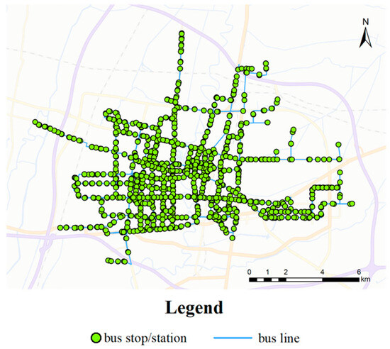
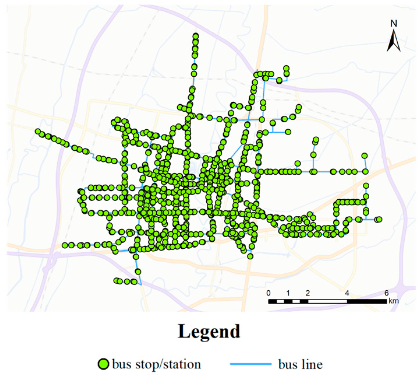
Cangzhou City, a third-tier city in Hebei Province, benefits from its strategic location within the developing Beijing–Tianjin–Hebei urban agglomeration. This study examines the PTN within Cangzhou City’s urban area. The line and stop data were obtained from the Python (version 3.11.7) package “Transbigdata” [42]. Accordingly, we retained bus lines and stops located in the city’s main urban area and selected urban–rural lines and stops, as shown in Figure 1. This segment of urban–rural lines provides services to pivotal towns in the peri-urban zone, which constitute core areas for prospective urban expansion. The dataset comprises 46 bus lines serving 573 unique stops. Forty-four lines form 22 bidirectional pairs, while Line 11 and Line 11B operate as loop services with nearly identical routings but different origin–destination nodes and are therefore treated separately. All geometries use WGS 1984 geographic coordinates and are projected to WGS 1984 Web Mercator (auxiliary sphere).
Figure 1.
Bus lines and stops within the study area.
Table 1 shows an example of bus line data obtained using “Transbigdata”. “Line” indicates the route number, “Dir” denotes the travel direction, and “Geometry” contains the line’s projected coordinate information.
Table 1.
Example of basic information of bus lines.
Table 2 illustrates an example of the stop data. In this table, “Stop_S” indicates the sequence of stops along the line’s direction, “Stop” refers to the stop’s name, and “Geometry” includes the stop’s projected coordinate information.
Table 2.
Example of basic information of bus stops.
3.2. Acquisition of Dynamic Data
The dataset was provided by Cangzhou Public Transport Group Co., Ltd., Cangzhou, Hebei, China. Passenger boarding records that allow macroscopic identification of peak, off-peak, and trough periods in bus operations. Bus GPS traces are included to determine vehicle arrival and departure events. The data are dated 12 April 2023, a Wednesday. Figure A1 shows the bus GPS data volume for each weekday of that week. The variance of daily volumes is 39,264.41, and the mean is 2,686,875. The Wednesday value is closest to the mean. No major festivals or adverse weather occurred that day, so it provides a representative snapshot of typical passenger travel and bus operations.
Table 3 shows an example of the passenger boarding data; “CardID” denotes individual passengers and “Time” records their boarding times.
Table 3.
Examples of passenger boarding data.
Table 4 provides an example of bus GPS data. In this table, “BusID” identifies different buses, “Speed” indicates the bus’s speed at a specific point, and “Geometry” denotes the vehicle’s projected coordinate position.
Table 4.
Examples of bus GPS data.
3.3. Data Processing
Data processing in this study was implemented using Python programming within Visual Studio Code (version 1.92.2) and ArcGIS software (version 10.2).
3.3.1. Processing of Line and Stop Data
The line and stop data obtained via the “Transbigdata” package were updated and differ from the April 2023 dataset. Consequently, some line and stop entries were corrected using bus GPS traces to align the lines with actual vehicle trajectories. The revised results are shown in Figure 1.
3.3.2. Processing of Passenger Boarding Data
This study uses only the passenger boarding records for the selected lines. These records were aggregated on an hourly basis to assess variations in bus passenger trips over the course of the day.
3.3.3. Bus Operation Data Processing
Data cleaning. Bus arrival and departure data at stops were derived through a multi-step processing workflow.
Step 1: A 100 m buffer was created around each stop, and bus GPS records on the same line and direction were intersected with this buffer to extract vehicle traces within 100 m of each stop. As shown in Figure A2, the 100 m buffer captures buses accelerating to the maximum speed (40 km/h) or decelerating at origin, terminal, and intermediate stations.
Step 2: Bus GPS data were screened by speed. According to Figure A3, when the speed threshold was 15 km/h, the distance between the buses and the station was smallest at vehicle entry and exit, and the distance standard deviation was also relatively low. The proportion of extracted entry and exit data was closest to 1. Therefore, at the starting and terminal stations, the speed threshold was set to 15 km/h. In Figure A4, “Mean Distance” denotes the average distance of extracted buses at entry and exit of intermediate stops under the given speed thresholds, and “Data Size” denotes the amount of entry and exit information. The Mean Distance changes markedly between the 12 km/h and 15 km/h thresholds, reflecting the effect of bus movement. Meanwhile, at the 15 km/h threshold, a relatively large amount of data were obtained, about 82% of the amount at 25 km/h. In conclusion, the speed threshold for intermediate stations was likewise set to 15 km/h.
Step 3: The initial data point at the origin station was retained to mark the vehicle’s departure time. For intermediate stops, both the first and last data points were kept to represent arrival and departure times, respectively. At the terminal station, the first data point was retained to indicate the vehicle’s arrival time.
Step 4: Each vehicle’s entry and exit times were aligned in the same row, grouping records by operational trip.
Following these procedures, we conducted a preliminary cleaning of the bus arrival/departure event logs, producing 94,210 GPS trajectory records. As shown in Table 5, Ta denotes the vehicle’s arrival time, Td denotes the departure time, and Trips indicates the number of operational trips.
Table 5.
Examples of cleaned bus GPS data.
Data repairing. Vehicle GPS signal errors and operator actions, such as failing to activate or prematurely deactivating the GPS device, can produce missing GPS records at certain stops or generate data that does not satisfy the predefined cleaning criteria. For example, if the driver does not switch on the GPS device at the origin stop, the GPS record for that stop may be absent for a given trip. Building on the methodological framework of Wang et al. [43], this study proposes a data-completion algorithm with the following processing steps:
Step 1: Compare the output from the previous stage with the stop/station list for the corresponding line directions to detect any missing stop/station information.
Step 2: For trips with missing data, first identify the stops or stations that lack information. Then determine whether the arrival and departure records for those stops are present in the previous or next trip of the same vehicle. If both adjacent trips contain the required records, compute the time difference between the arrival at the target stop and the departure from the upstream stop for each trip. Use the mean of these two time differences to estimate the missing arrival time. Apply the same procedure to estimate the departure time. If only one adjacent trip—either the previous or the next—contains the required data, use that single observation directly without averaging. If neither adjacent trip contains the stop information, proceed to Step 3.
Step 3: Search for arrival and departure information for the stop in other trips that occurred within the same hour. If such records exist, apply the calculation described above to estimate the missing times. If no records are found within the hour, assume the vehicle did not stop at that stop, and take no further action.
Step 4: Aggregate the complemented results on an hourly basis to support construction of the dynamic network.
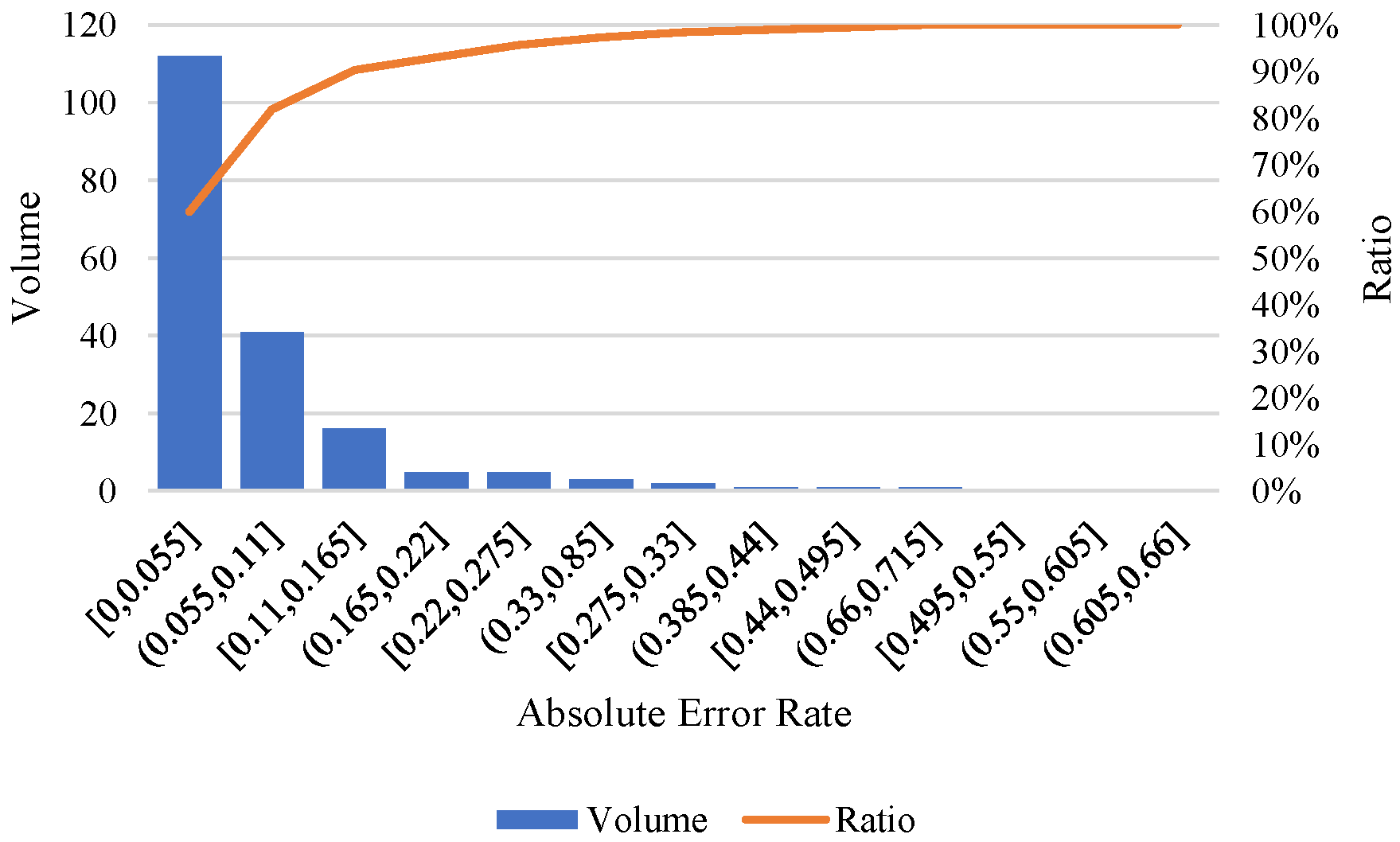
Using this complementation algorithm, we added 4347 new data entries. To illustrate the accuracy of the supplemented data, we examine the important Route 307. Figure A5 shows the distribution of absolute error rates in interstation running times between the complemented dataset and the original Route 307 data. Eighty percent of the values have errors below 10%.
Construction of adjacent-stop connections. Using the provided data, we derived the adjacency relationships between stops. Table 6 presents an example of these results. Here, “Stop_u” denotes the upstream stop in the direction of travel, and “Stop_d” denotes the downstream stop. “Time_interval” specifies the travel time between adjacent stops in seconds, and “Hour” indicates the hour when the data were collected.
Table 6.
Examples of connection relationships between adjacent stops.
4. Methods
In a static network, a bus route between two stops denotes a connection. In real operations, however, the number of vehicles running between adjacent stops fluctuates dynamically over time. Consequently, dynamic PTNs differ from static ones. For comparative analysis, this study used Gephi (version 0.10.1) to construct both static and dynamic networks and to compute their respective network indicators.
4.1. Static PTN
The L-space method builds a static, weighted bus network in which stops are nodes and edges join consecutive stops along the same route. Key aspects are that: (1) stop names are made unique by removing duplicates; (2) edge weights equal the actual line distances; and (3) the network is directed. Table 7 shows the associations between adjacent stops, with “Distance” reporting the line distance between them in meters.
Table 7.
The association relationship between adjacent stops in the static bus network.
4.2. DWDN I
To evaluate the evolving properties of nodes in the dynamic network, we construct DWDN I using the L-space method. Edge weight is defined as the hourly number of buses passing between adjacent stops [31]. The edge-weight calculation is as follows:
where wij(t) represents the weight of edge eij at the t-th hour, Lij denotes the set of all bus lines that pass eij, and indicates the number of vehicles on line l traveling from stop i to stop j.
4.3. DWDN II
When calculating path length and network diameter, using the number of vehicles between stops as the edge weight is of limited practical value and does not capture vehicle operating characteristics. Peak-hour congestion, for example, can cause buses to cluster on certain road segments, so a high vehicle count does not imply an efficient PTN. To address this, the present study builds DWDN II using the P-space method to define interstation connections in the public transport network. To enable assessment of operational efficiency, the average running time is employed as the edge weight. The edge-weight calculation method is as follows:
where denotes the average travel time from stop i to stop j during the t-th hour, serving as the edge weight in DWDN II, Tt,k(i, j) represents the actual travel time (in seconds) for the k-th vehicle traveling between stops i and j within the t-th hour, and Nt(i, j) indicates the number of vehicles traveling from station i to station j during the same hour.
In constructing the two aforementioned dynamic networks, lines and stations were categorized into directions 0 and 1 to facilitate a comparison of the directional differences within the dynamic networks.
4.4. Indicators Used
4.4.1. Degree
The degree of a node, defined as the number of its neighbors, is a common metric for node importance. In a static network, a node’s degree is constant. In a dynamic network, however, the number of vehicles traveling between adjacent nodes and the travel times between stops change over time, which alters the network’s connections and thus the node degrees.
4.4.2. Weighted Degree
The weighted degree applies to weighted networks. In this study, we compute the weighted degree only for DWDN I; it equals the number of vehicles passing between a node and its neighbors within one hour.
The weighted-degree distribution P(k) is the fraction of nodes in DWDN I with weighted degree k, formally expressed as
where N(k) denotes the count of nodes with a weighted degree of k within the network, while N signifies the total number of nodes present in the network.
An indicator for identifying a scale-free network is that its cumulative weighted-degree distribution adheres to a power-law distribution.
4.4.3. Clustering Coefficient
The clustering coefficient is defined as the ratio of the actual number of edges connecting a node’s neighboring nodes to the maximum possible number of such edges, as shown in Equation (4).
where ki represents the degree of node i, and xi denotes the number of actual edges connecting the neighboring nodes of node i.
The clustering coefficient measures the closeness of nodes. Specifically, a larger clustering coefficient indicates a higher degree of closeness between a node and its neighboring nodes.
The overall clustering coefficient C of the network is calculated as the mean of the clustering coefficients for all nodes within the network. C can be defined as
4.4.4. Average Path Length
The shortest path between nodes i and j is defined as the minimum number of nodes (path length) along the connecting route. The average path length is the mean of these shortest-path lengths over all node pairs in the network.
4.4.5. Network Diameter
The network diameter is defined as the longest of the shortest-path lengths between any pair of nodes within the network.
4.4.6. Small-World Coefficient
Calculating the small-world coefficient yields stronger quantitative evidence for the PTN’s small-world characteristics. We adopt coefficient ω [44] as the numerical indicator of small-world topology, defined by the following formula:
where Lrand represents the average path length of the corresponding random network, and Clatt represents the clustering coefficient of the corresponding lattice network.
4.4.7. Network Efficiency
Network efficiency is the average of the reciprocals of the shortest paths between all pairs of nodes in the network. Therefore, this indicator is selected to calculate the transportation efficiency of the P-space network.
4.4.8. Centrality Indicators
In the bus network, centrality indices are often used to measure the importance of stations [8,26,34]. The centrality indices considered in this paper include three types: betweenness centrality (BC), closeness centrality (CC), and eigenvector centrality (EC). Among them, BC is used to measure the number of shortest paths passing through the corresponding bus station. CC is measured by the reciprocal of the average shortest path from the corresponding station to other stations. The larger its value is, the higher the importance of the corresponding node is. EC emphasizes the influence of the number and importance of neighbor nodes on the importance of the corresponding node. Since both BC and CC are affected by the shortest path, the edge weight used in the network model during calculation is the average running time between stations. Correspondingly, since EC is affected by the node degree, the edge weight used during calculation is the number of passing buses between stops.
5. Results
5.1. Division of Bus Operation Stages
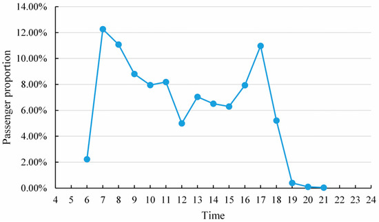
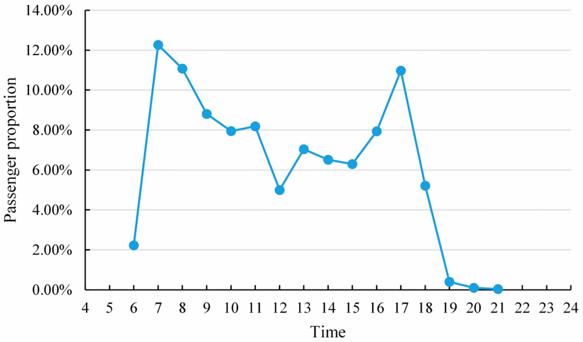
By aggregating passenger boardings hourly, we examined diurnal variation in bus trips. Figure 2 shows each period’s share of the total daily boardings. The data indicate a morning peak between 7:00 and 8:00, an evening peak at 17:00, off-peak intervals from 9:00 to 10:00 and from 14:00 to 15:00, and a midday trough at 12:00.
Figure 2.
Time-varying characteristics of boarding passengers.
5.2. Results of Static-Network Indicators
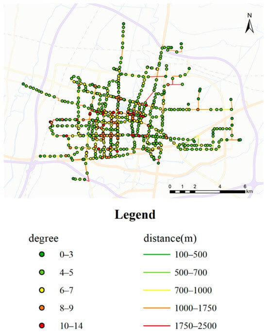
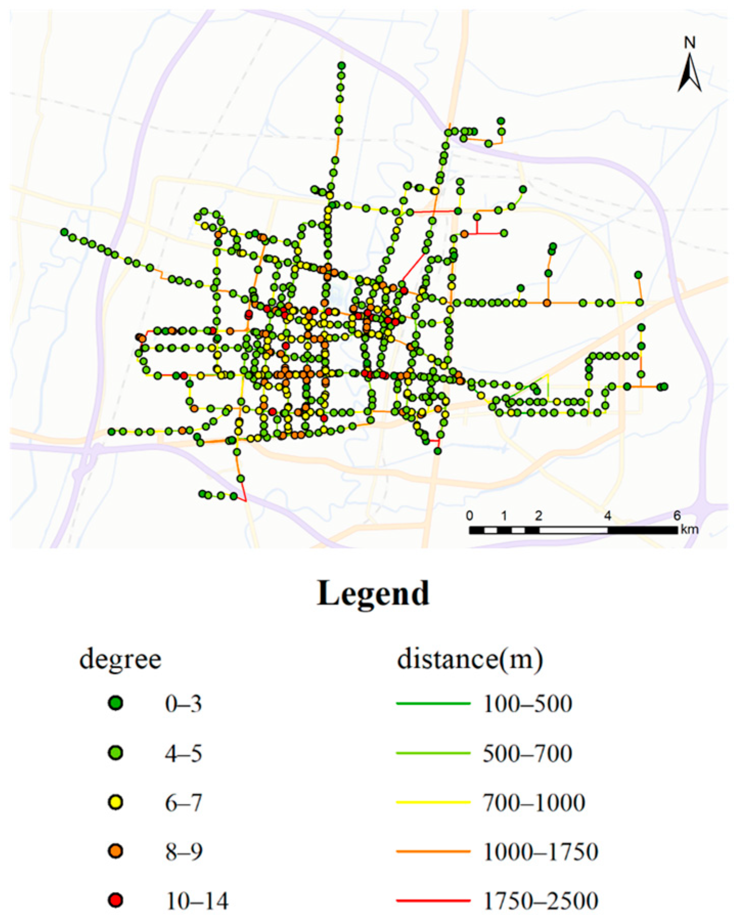
Figure 3 displays the spatial distribution of static-network node weighted degrees and line weights. Stations with high weighted degrees concentrate in the urban core, where they align primarily along three east–west roads, one north–south road, and within a mixed-use area. From north to south, the east–west roads are Xinhua Road, Jiefang Road, and Huanghe Road; the north–south road is Fuyang Avenue; and the mixed-use area is the “Cangzhou People’s Hospital—Jianxin Commercial Pedestrian Street” complex. Line segments with large stop spacing are mainly located at the city edge.
Figure 3.
Visualization results of the static PTN.
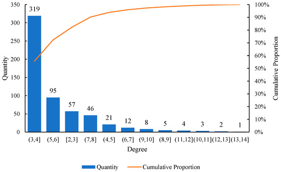
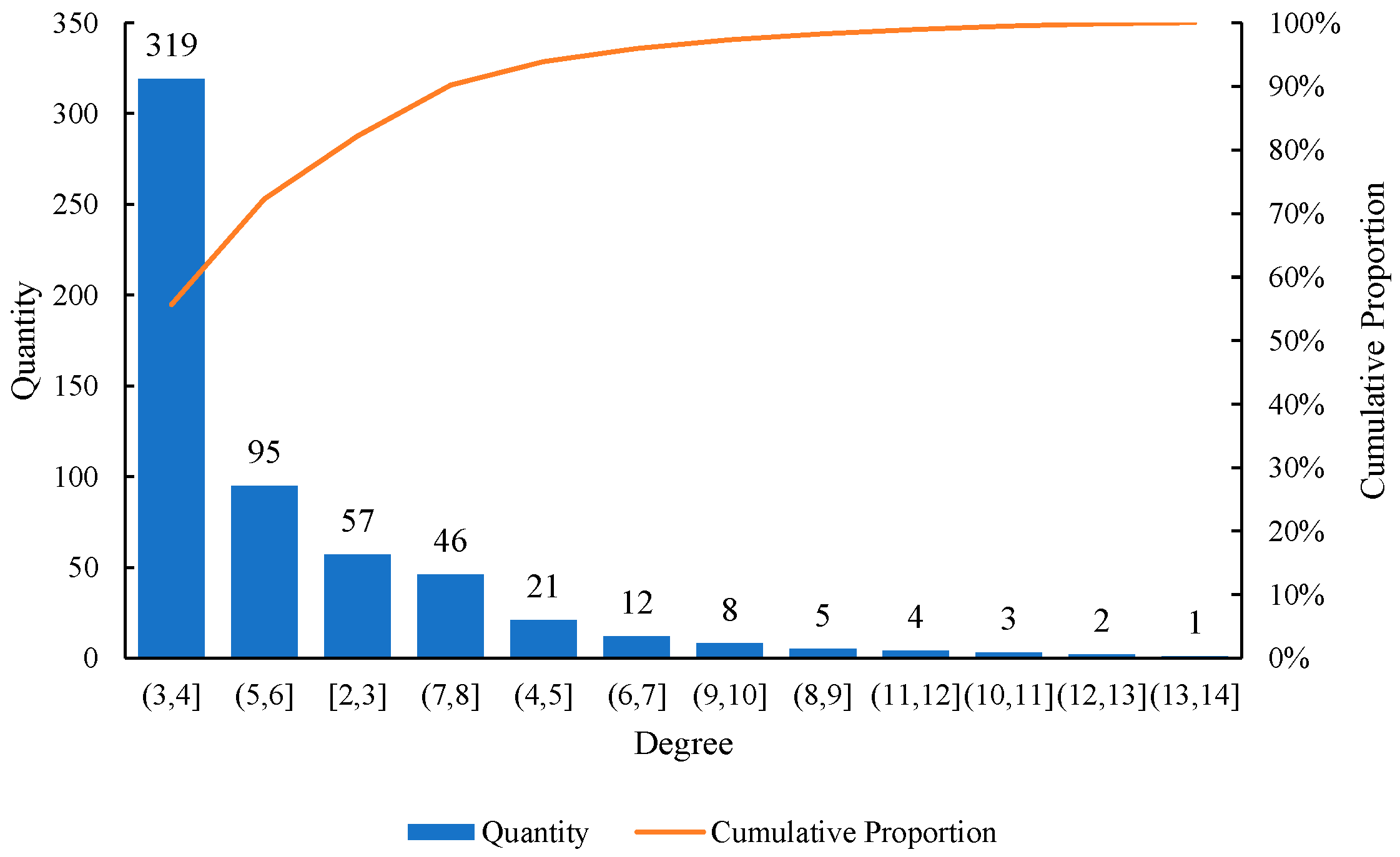
Figure 4 shows the degree distribution of the static network. Stops with degrees of 4 and 6 are the most common, accounting for more than half of all stops. The network’s average degree is 2.419, indicating that each stop typically connects to 2 or 3 neighboring stops. The average weighted degree is 1450.05, which corresponds to an average distance of about 1450 m between adjacent stops. The network diameter is 62, so the longest shortest path can include up to 62 stops. The average path length is 17.318, meaning that, on average, 17 stops are reachable along the shortest paths. The average clustering coefficient is 0.085.
Figure 4.
Degree distribution of the static network.
5.3. Results of DWDN I
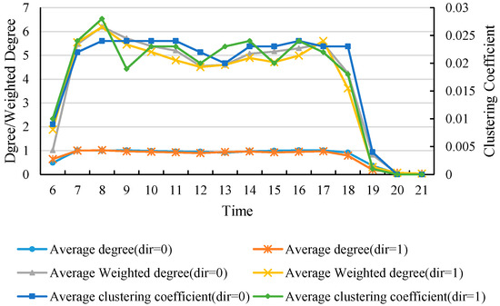
For DWDN I, we computed three network metrics: degree, weighted degree, and clustering coefficient. Figure 5 shows the temporal variations in the network’s average degree, average weighted degree, and average clustering coefficient. All three metrics closely track passenger boarding volume and display an “M”-shaped pattern. Table A1, Table A2 and Table A3 report the comparative analysis of clustering coefficients between the static network and DWDN I. The results indicate significant differences in clustering between the two network types, whereas temporal variations in clustering within the dynamic network are not significant.
Figure 5.
Temporal variations in three indicators of DWDN I.
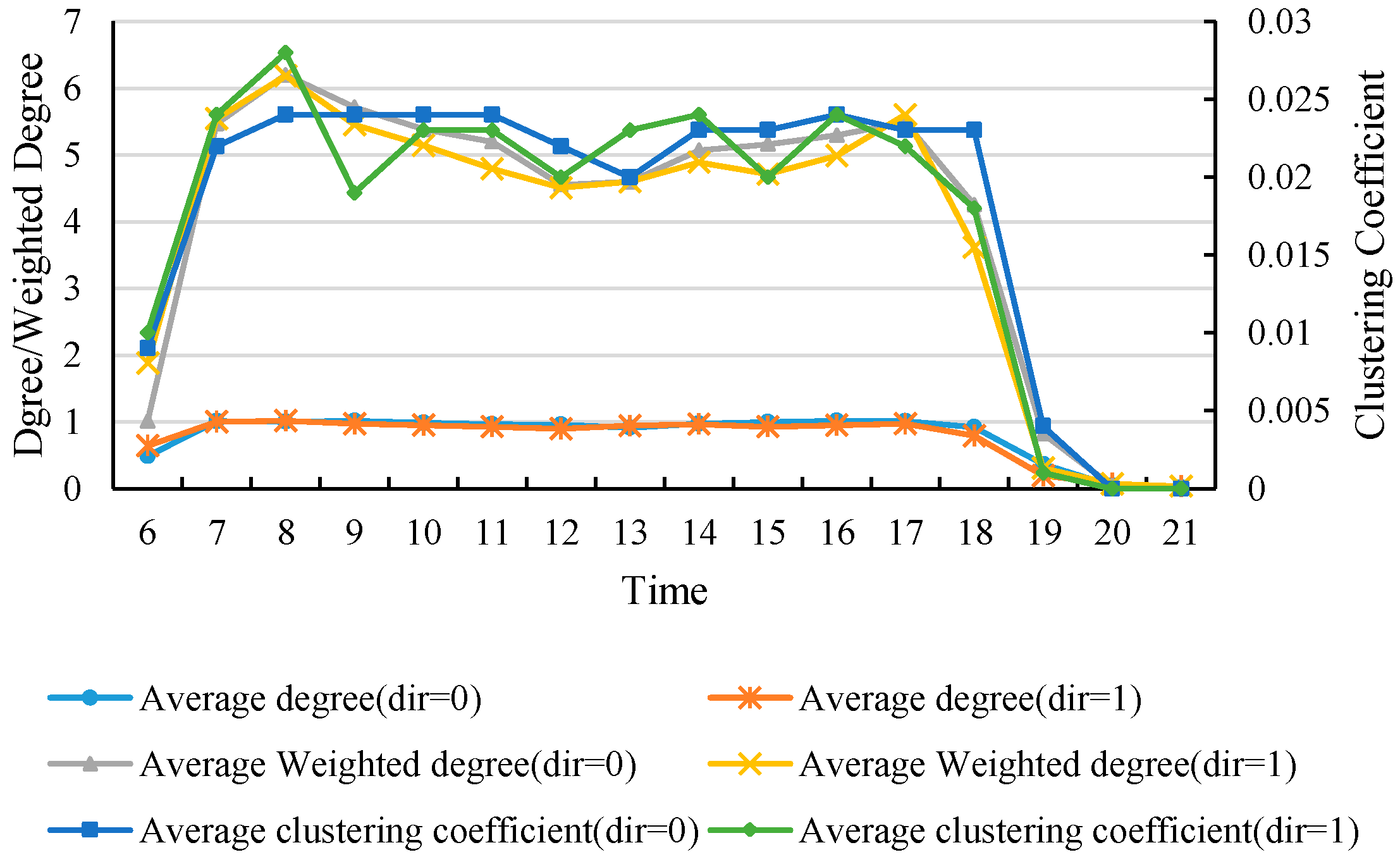
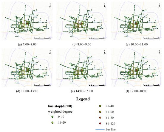
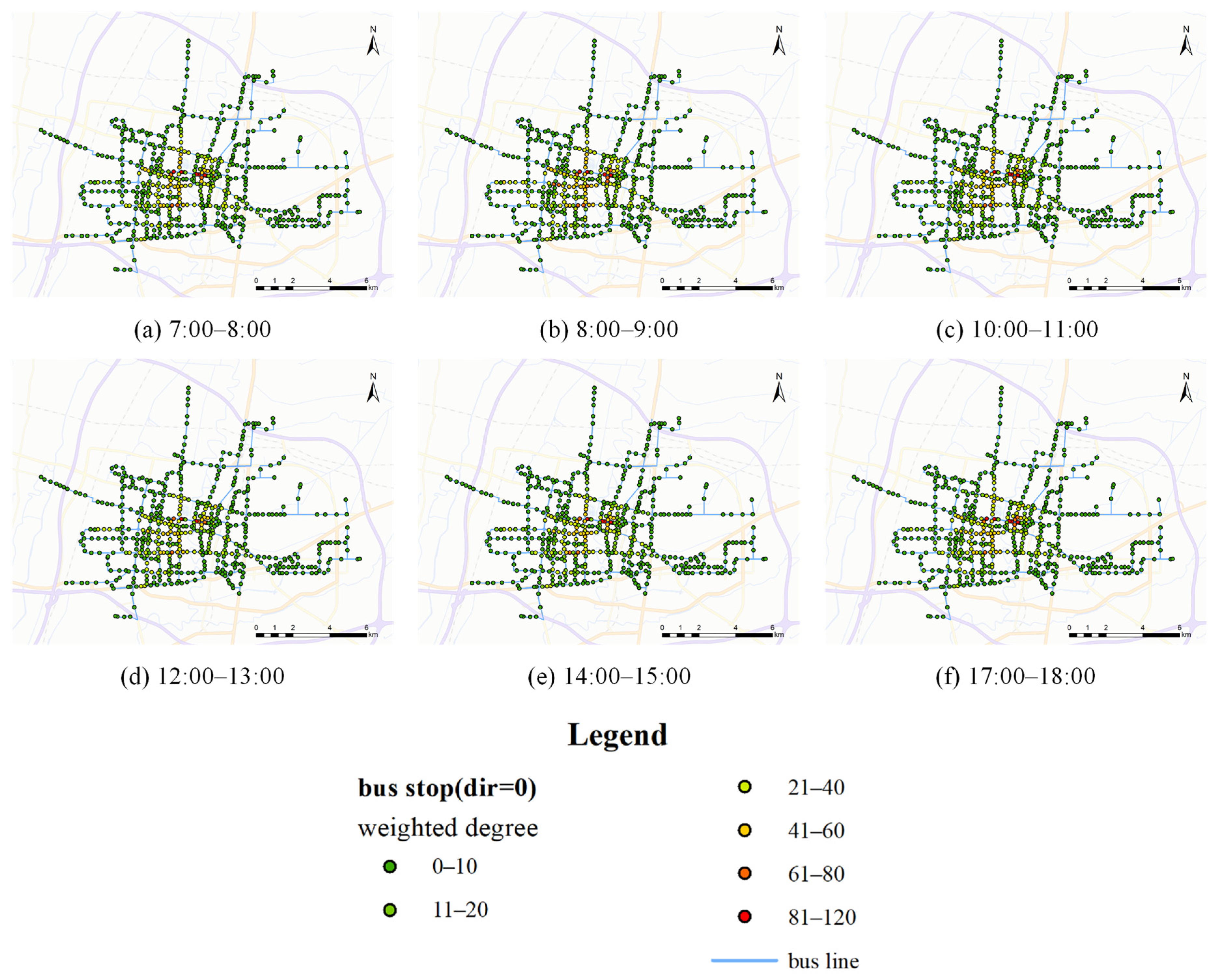
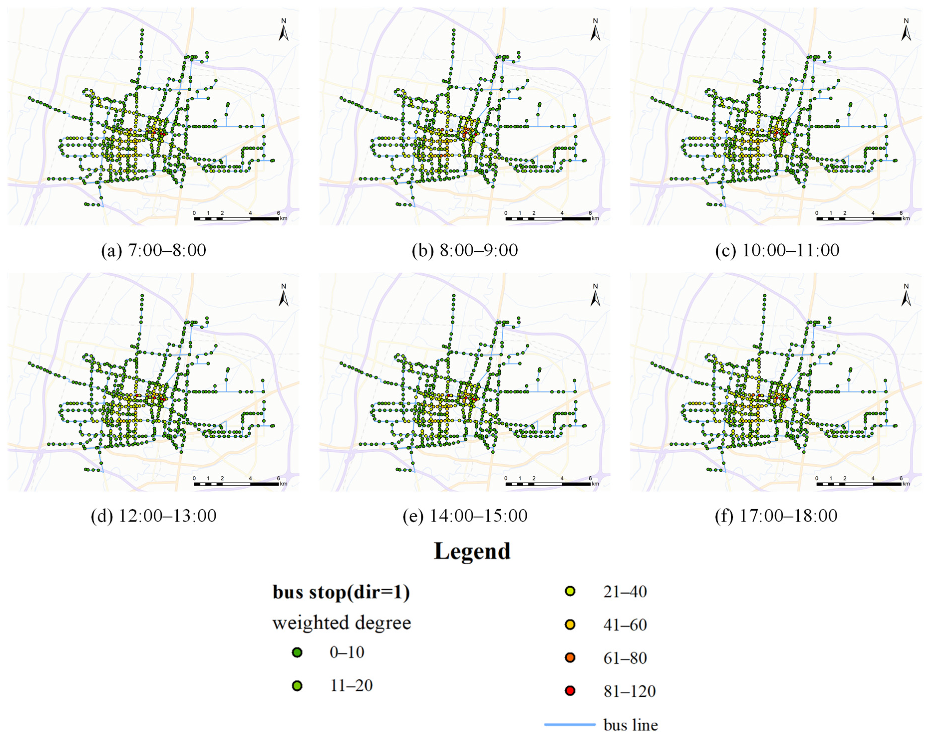
To examine the spatiotemporal distribution of weighted degrees, we used ArcGIS to map the weighted degrees of bus stops in directions 0 and 1 for six time windows: 7:00–8:00, 8:00–9:00, 10:00–11:00, 12:00–13:00, 14:00–15:00, and 17:00–18:00, as shown in Figure 6 and Figure 7. The results reveal several notable patterns. First, as in the static network, stations with high weighted degrees in DWDN I remain concentrated along three roads and within one mixed-use area. Second, the spatial distribution of weighted degrees differs between directions 0 and 1. For example, stops on Yongji Road in direction 0 exhibit relatively higher weighted degrees during most time windows. In addition, stops with dir = 0 and dir = 1 near the Cangzhou West Station office complex show elevated weighted degrees during 8:00–9:00 and 17:00–18:00, respectively. These two periods correspond to the primary commuting hours.
Figure 6.
Spatial distribution of weighted degrees in different time periods (dir = 0).
Figure 7.
Spatial distribution of weighted degrees in different time periods (dir = 1).
We used global Moran’s I to assess spatial autocorrelation of the weighted degrees in both directions. Results are presented in Table 8 and Table 9. For the network with dir = 0, Moran’s I ranges from 0.52 to 0.64 across time periods, values that are positive and substantially above the expected index E (I). The Z-values exceed 1.96 in every period and p < 0.01, indicating extremely significant positive spatial autocorrelation of bus weighted degrees in the dir = 0 direction and clear spatial clustering. Moran’s I peaks at 0.639 and 0.628 during 10:00–11:00 and 12:00–13:00, respectively, indicating the strongest clustering then. For the network with dir = 1, Moran’s I ranges from 0.386 to 0.608 and is also mostly positive. In the 7:00–8:00 period, Z = 1.904 and p = 0.057, which approaches the conventional significance threshold; in the remaining periods, Z > 1.96 and p < 0.05, indicating significant or highly significant positive spatial autocorrelation. Overall, the dir = 1 direction also shows clear spatial clustering, although its intensity and statistical significance are slightly lower than those for dir = 0.
Table 8.
Results of weighted-degree spatial autocorrelation analysis (dir = 0).
Table 9.
Results of weighted-degree spatial autocorrelation analysis (dir =1).
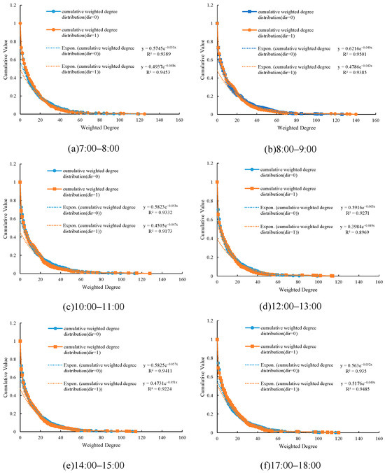
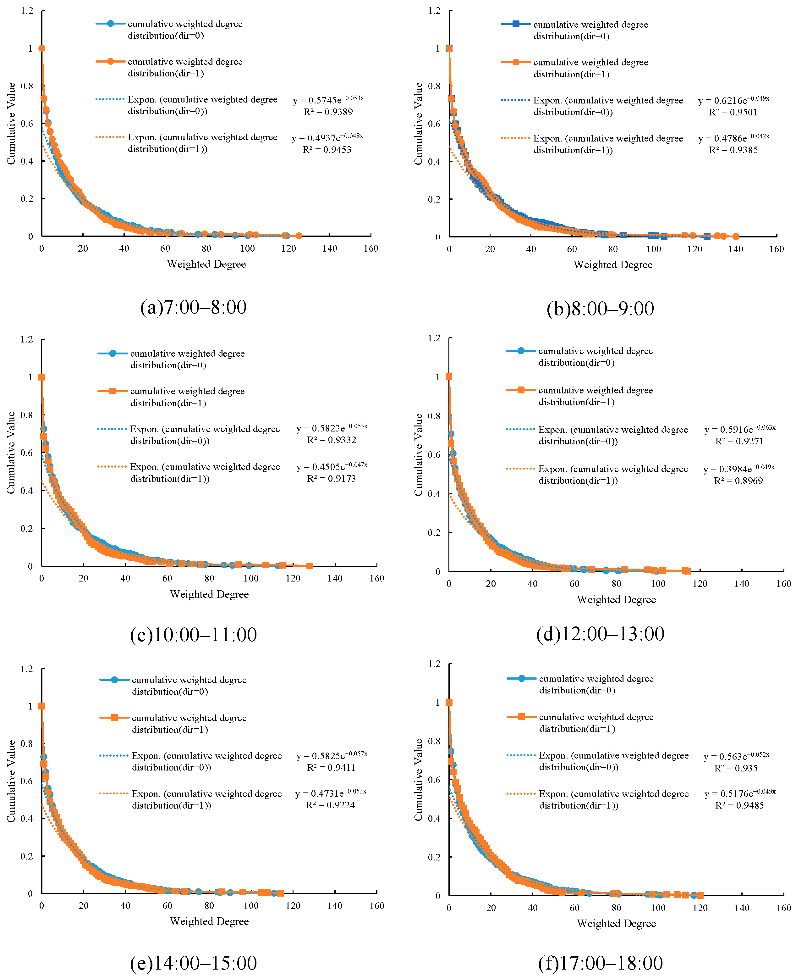
Figure 8 shows the cumulative weighted-degree distributions for the six specified time periods, with exponential fits producing R2 values greater than or close to 0.9 in all cases. The results indicate that DWDN I does not exhibit a scale-free topology.
Figure 8.
Cumulative weighted-degree distribution in each time period.
5.3.1. Results of DWDN II
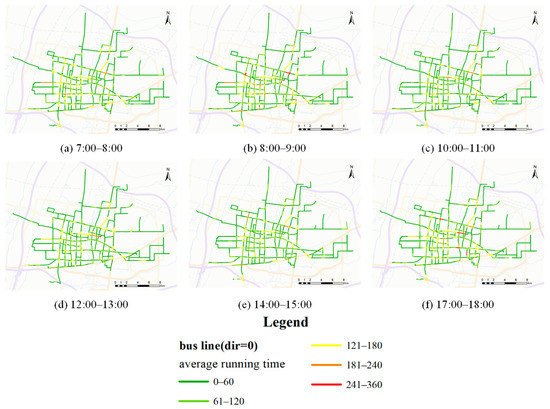
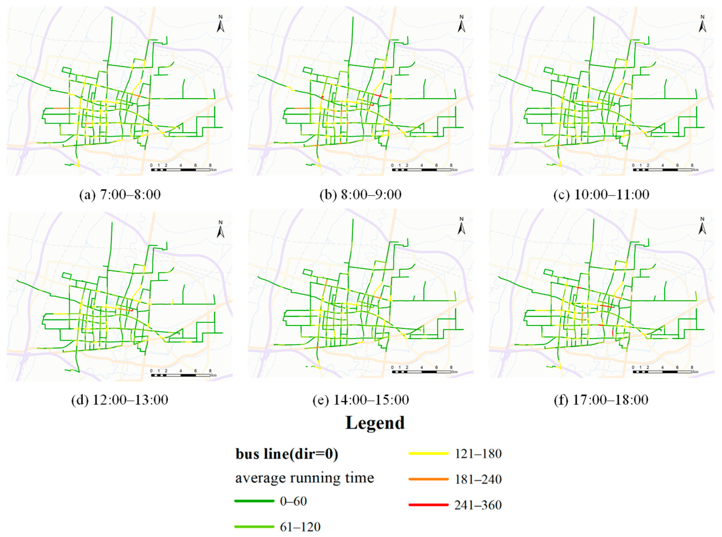
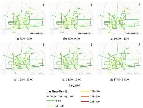
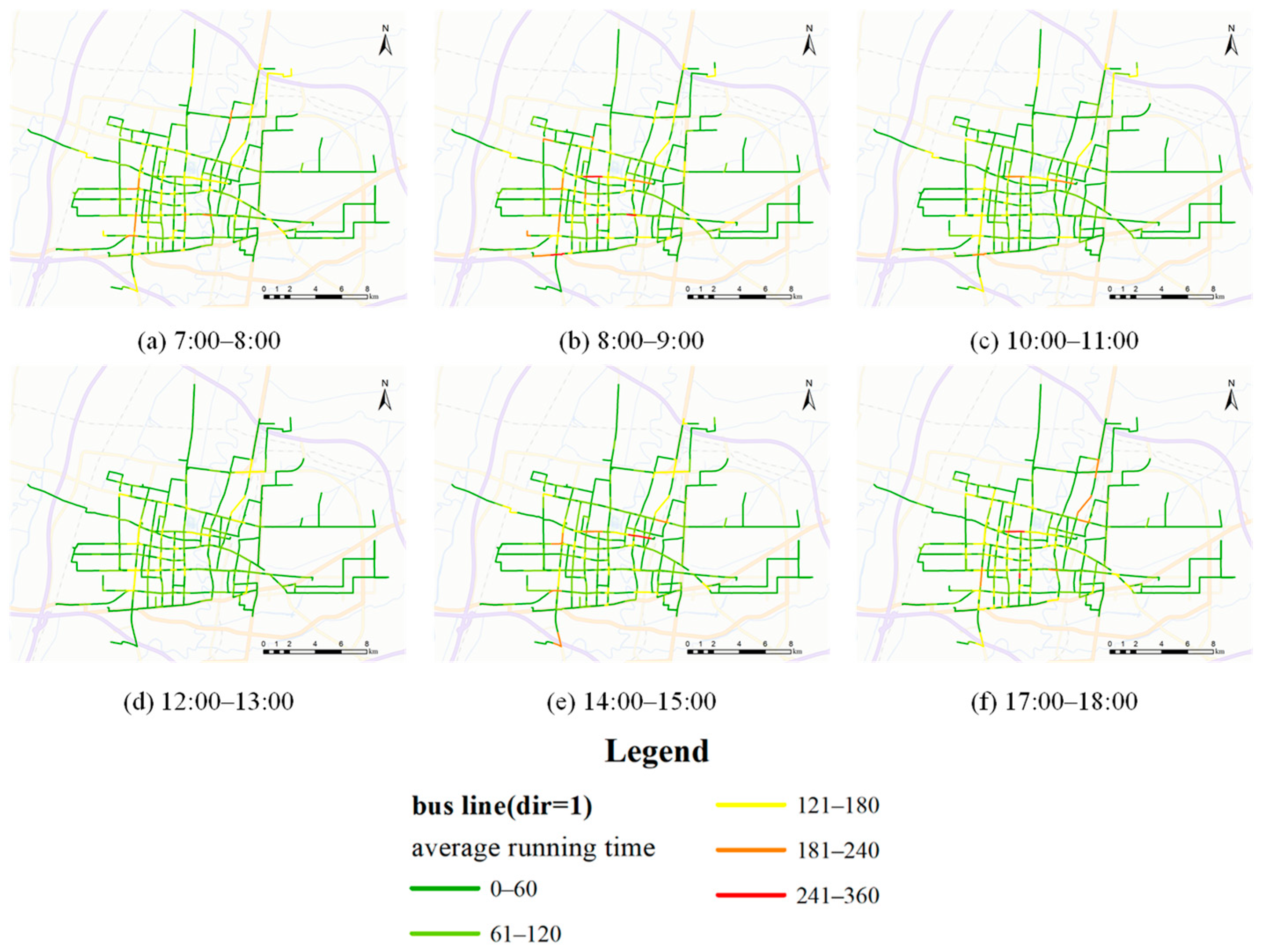
Figure 9 and Figure 10 show ArcGIS visualizations of average bus running times (seconds) between adjacent stops for each time period. The maps indicate consistently longer inter-stop travel times across all periods in three zones: the west side of the Yongji Road–Qiantong Avenue intersection (where Yongji Road passes over the railway), Xinhua Road (from Huabei Commercial Building to Cangzhou Railway Station), and the area around the Neurology Branch of Cangzhou Central Hospital.
Figure 9.
Spatial distribution of average travel time between adjacent stops (dir = 0).
Figure 10.
Spatial distribution of average travel time between adjacent stops (dir = 1).
Furthermore, a global spatial autocorrelation analysis was conducted on the average running time, and the results are shown in Table 10 and Table 11. In sharp contrast to the significant agglomeration characteristics of the weighted degree, the average running time between stations does not exhibit obvious and stable spatial agglomeration characteristics and shows significant differences in different directions.
Table 10.
Results of average running time spatial autocorrelation analysis (dir = 0).
Table 11.
Results of average running time spatial autocorrelation analysis (dir = 1).
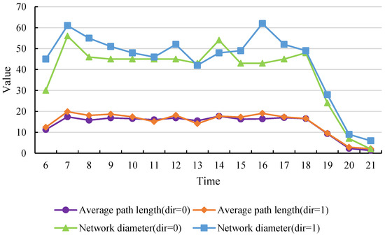
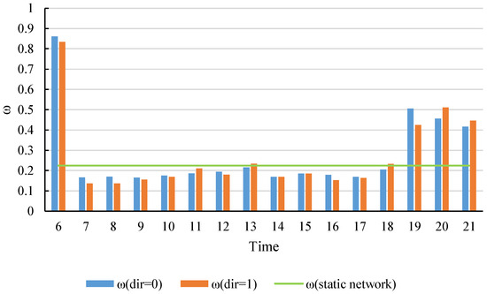
Figure 11 shows temporal changes in average path length and network diameter for both directions. The average path lengths in the two directions follow similar trends, whereas the network diameters display clearly different patterns.
Figure 11.
Temporal characteristics of average path length and network diameter.
5.3.2. Small-World Characteristics
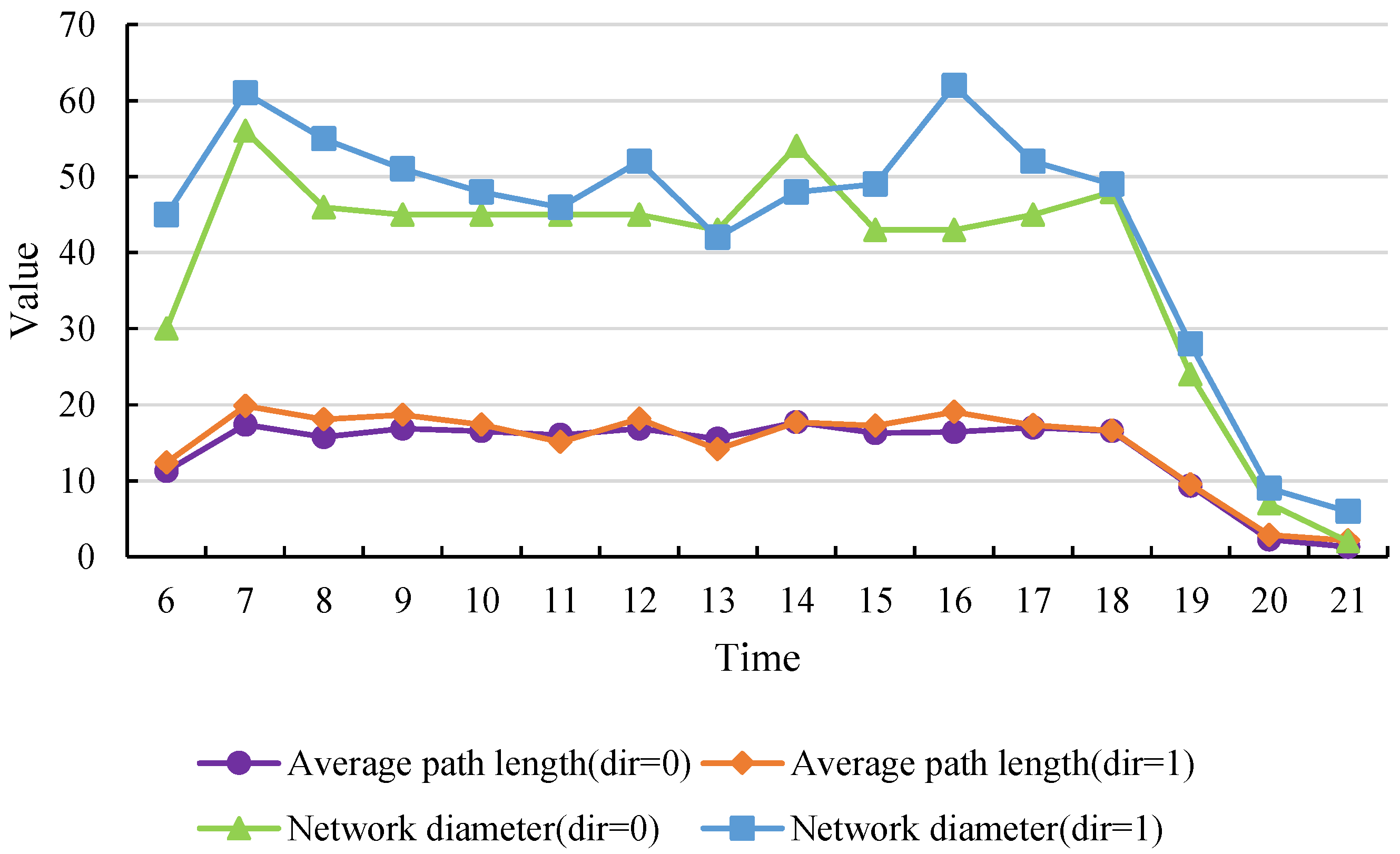
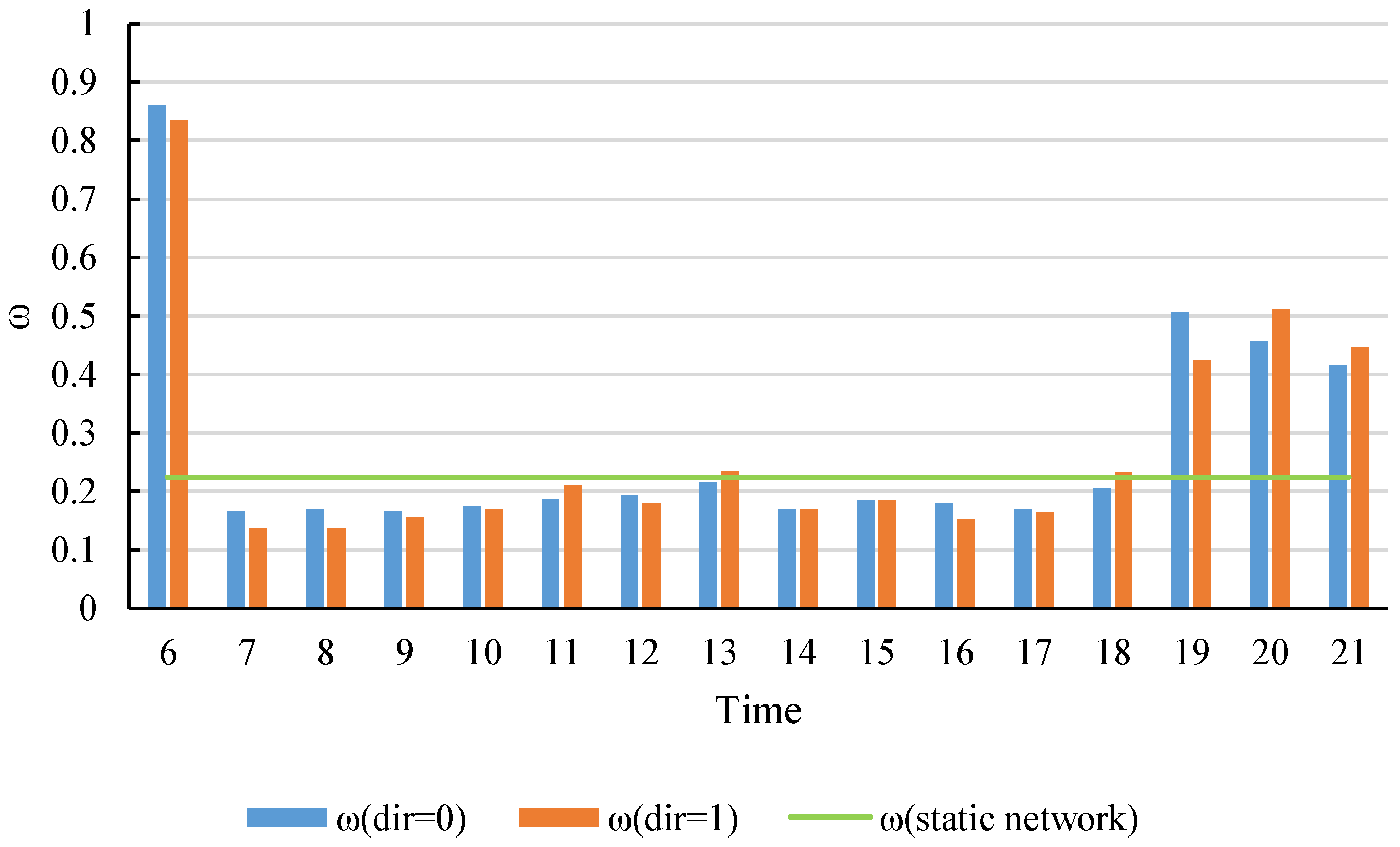
Figure 12 compares the small-world coefficients of the dynamic and static networks. Over the full-day operation period, the dynamic network’s small-world coefficient ω follows an inverted “M” pattern. From 7:00 a.m. to 5:00 p.m., ω first rises and then falls, peaking at 13:00. For most of the daytime, the dynamic network’s ω is lower than that of the static network, indicating that the dynamic network exhibits stronger small-world characteristics.
Figure 12.
Small-world network coefficient ω contrast.
5.3.3. Time-Varying Network Efficiency Characteristics
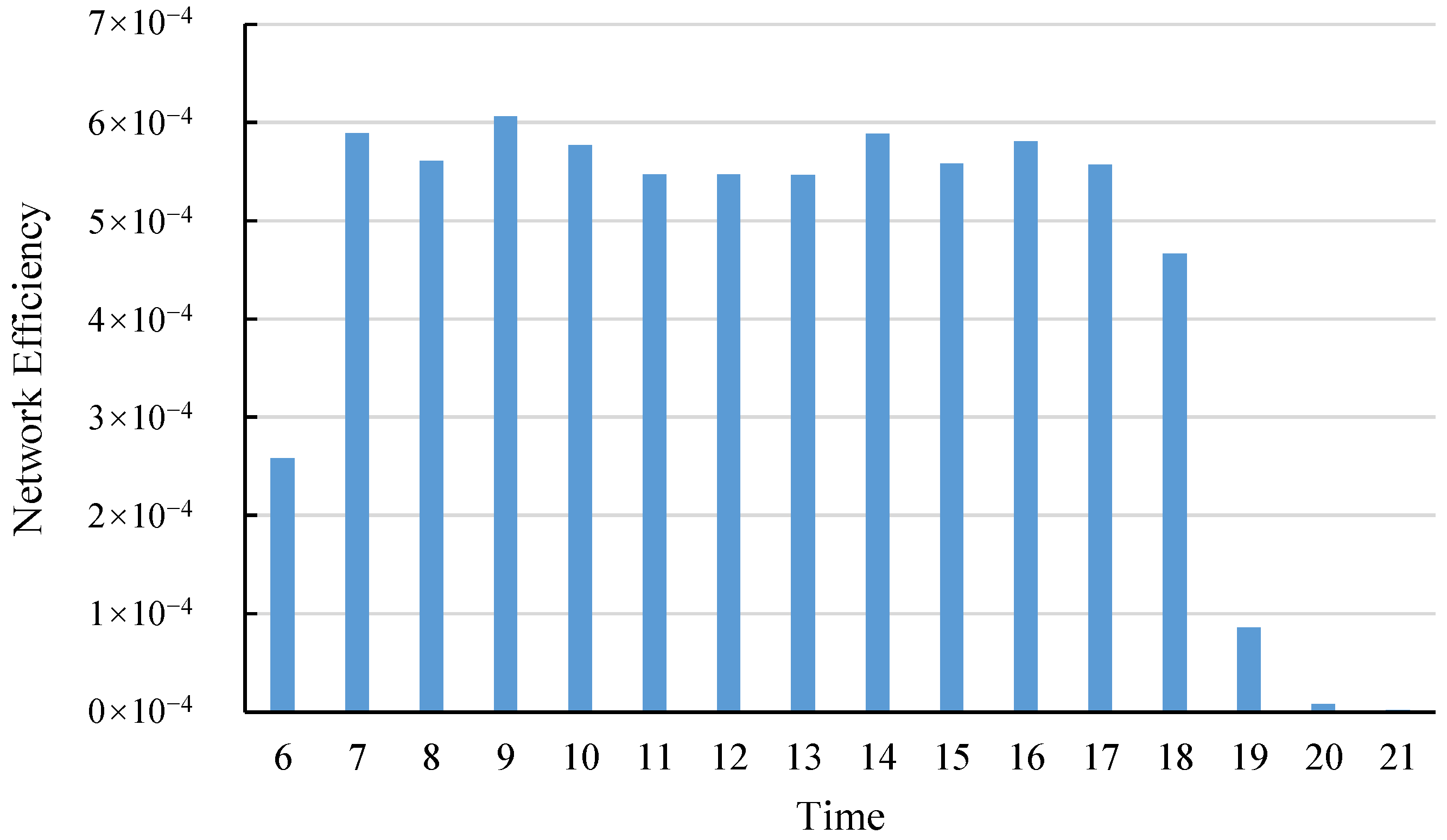
In this study we calculated the bus network’s efficiency for 16 time periods from 6:00 to 21:00 on an hourly basis. The results are shown in Figure 13. Over the course of a day, the network efficiency follows an approximately M-shaped pattern. The midday decline in network efficiency, however, is less pronounced than the corresponding decrease in passenger flow, and the metric remains relatively stable at a high level. Overall, the temporal variation in network efficiency aligns with the operational schedule of buses in Cangzhou. Some lines begin service around 6:30, and most lines cease operation after 18:00. Using the network efficiency at 16:00 as an example, the average running time between stations is 35 min. Thus, for most of the day a passenger can expect to reach another station in the network in about 30 min on average. This value satisfies the requirement in the standard [45] that the maximum bus travel time 7.0 for cities with a population of 500,000–1,000,000 be 40 min.
Figure 13.
Network efficiency during different time periods.
5.3.4. Spatiotemporal Distribution of Key Stops
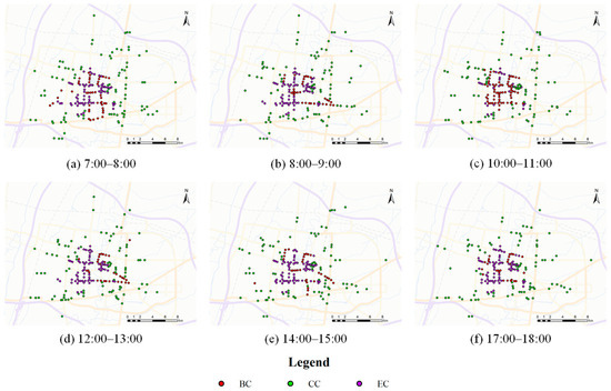
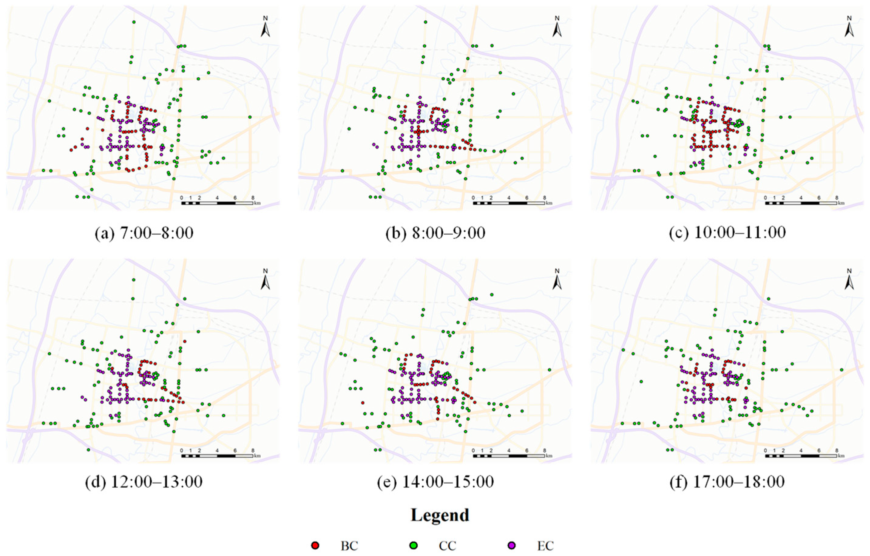
The three centrality measures were computed using Gephi software. Figure 14 displays the top 50 bus stops for each measure: BC, CC, and EC. The spatial distribution of these stops remains largely stable across time periods. Stops with high BC and EC values cluster near the city center, while stops with high CC values are dispersed toward the urban periphery.
Figure 14.
Spatial distributions of the top 50 bus stops ranked by three centrality indicators.
6. Discussion
This study examines the public transit network (PTN) of Cangzhou City, a third-tier city in Hebei Province, China, to offer an exploratory case for small-city transit research. Using passenger boarding data, we identified peak, normal, and off-peak bus operation periods. After cleaning and completing bus GPS records, we built the static PTN and DWDN I with the L-space method and DWDN II with the P-space method. We then used Gephi to compute key metrics, including degree, weighted degree, clustering coefficient, average path length, network diameter, and centrality indicators. Comparison of the spatiotemporal distributions of these metrics produced the following findings:
6.1. Public Transit Supply
The daily pattern of boarding passengers on Cangzhou buses typically follows an “M” shape. The morning peak occurs from 7:00 to 9:00, and the evening peak from 17:00 to 18:00. This pattern reflects the fact that many office workers in Cangzhou begin work at 8:00 or 8:30 and end their workday around 17:30 in the spring. There is no midday peak in bus travel, indicating that commuters generally do not return home at noon.
The degree, weighted degree, and clustering coefficient for DWDN I, together with the average path length, network diameter, and network efficiency for DWDN II, all follow an M-shaped temporal pattern, whereas the small-world coefficient ω follows an inverted M-shaped pattern. These patterns consistently reflect dynamic adjustments in daytime bus supply in Cangzhou City in response to passenger flow. Specifically, during peak hours an increased vehicle supply strengthens connectivity among stops, raises node degrees and network efficiency, and accentuates the network’s small-world characteristics. Conversely, during off-peak hours a reduced vehicle supply lowers node degrees and network efficiency and weakens or eliminates the network’s small-world properties.
From a spatial standpoint, stops with high weighted degrees concentrate in zones of intense passenger activity. These include the Neurology Branch of Cangzhou Central Hospital on Xinhua Road, the “Huabei–Tongtian” commercial and administrative cluster on Jiefang Road, the Cangzhou Integrated Traditional Chinese and Western Medicine Hospital area on Huanghe Road, the Cangzhou Cultural and Art Center and Yuegangcheng Commercial Area on Fuyang Avenue, and the comprehensive area of “Cangzhou People’s Hospital—Jianxin Commercial Pedestrian Street”. This indicates that more buses are provided in areas with high intensity of bus passenger flow generation and attraction.
The findings indicate a strong spatiotemporal alignment between bus-route design and bus scheduling in Cangzhou City, which improves the utilization of bus resources.
6.2. Network Characteristics
In this study, betweenness centrality (BC) and eigenvector centrality (EC) measure the performance of stops in terms of shortest paths and bus flow respectively. The central urban area is the core functional area of the bus network. The top 50 stations ranked by both indicators are stably concentrated in the area near the city center, which confirms the crucial role of central area stops in the bus network. Among them, the distribution of stops with high BC values indicates that central area stops are the core nodes of shortest paths and undertake important transfer functions. The distribution of stops with high EC values shows that central area stations form strong connections relying on a larger bus flow. On the other hand, however, the exponential distribution of the weighted degree indicates that the dynamic bus network does not possess the attributes of a scale-free network—that is, the hub role of stations with high weighted degrees in the network is not obvious. Nevertheless, this also enables the PTN to exhibit stronger robustness under the influence of bad weather, road construction, and traffic accidents.
The observed clustering of stations with high CC values around the urban core contrasts with prior studies [6,8]. CC quantifies a node’s accessibility to all other nodes, so high-CC stops are typically expected in central areas. Our analysis indicates that these particular stops have relatively few network connections, primarily serve local neighborhoods, and operate under conditions with limited traffic congestion, which yields relatively high travel speeds.
6.3. Cross-City Comparison
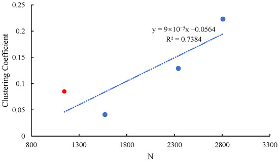
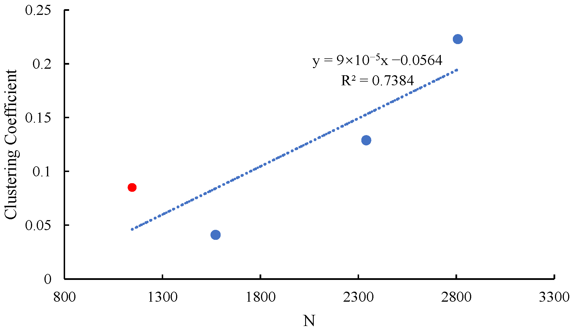
Different methods for constructing urban bus-network models have hindered direct comparison of network parameters across studies. The clustering coefficient, a commonly used metric in PTN analysis, was examined here using published results for Changsha [14], Xi’an [21], and Ningbo [32] as benchmarks. Figure 15 shows a clear positive linear relationship between the clustering coefficient and the number of bus stops N across the four cities. The Cangzhou data point (red) lies above the fitted line, indicating that Cangzhou’s clustering coefficient exceeds the value predicted for networks with the same number of stops. This suggests that, despite its smaller size, Cangzhou’s network maintains relatively dense local connections rather than exhibiting a proportional decrease in local clustering with scale.
Figure 15.
Relationship between the clustering coefficient and the number of bus stops.
6.4. Problems in Bus Operation
Analysis of the spatial distributions of weighted degree and of average running time between stations shows that stations with high weighted degrees and segments with long average running times are spatially coupled. This pattern indicates that traffic design and the built environment affect bus operational efficiency. Bus operators can improve the traffic efficiency of important stations by implementing stricter bus lane strategies, optimizing road cross-section design, and implementing bus priority signal control measures.
7. Conclusions
Research on urban PTNs in China has focused primarily on first-tier cities, such as Beijing, Shanghai, and Shenzhen, and on selected second-tier cities, including Changsha, Ningbo, and Harbin. In contrast, PTNs in third-tier cities have received far less attention. Prior work has emphasized complex-network attributes of bus systems while paying insufficient attention to the spatial patterns of corresponding indicators. Public transport in third-tier cities is important for serving low-income groups and the elderly, reducing emissions, and maintaining social equity. This study examines the PTN of Cangzhou, a third-tier city, to provide an exploratory case for research on bus networks in smaller urban centers. We constructed a static network using the L-space method and DWDN I, and built DWDN II using the P-space method. To characterize directional dynamic PTNs (dir = 0 and 1), we analyzed network measures including degree, weighted degree, clustering coefficient, average path length, and network diameter. The study yields several conclusions.
- (1)
- Temporal and spatial alignment between bus supply and demand: At the macro level, the analysis shows that Cangzhou’s bus routes and vehicle schedules generally match passenger needs. Temporally, the time series of average degree, weighted average degree, average clustering coefficient, network diameter, average path length, and network efficiency of the dynamic PTN follow the “M”-shaped pattern of passenger card swipes for boarding, indicating that bus resources are adjusted dynamically in response to fluctuating travel demand. Spatially, stops with high weighted average degrees cluster around hospitals, commercial areas, and administrative offices, which function as the primary traffic generators and attractors.
- (2)
- Spatial distribution of key stations: Points with high weighted degree, CC, and EC values are concentrated in the urban core. Spatial autocorrelation analysis shows that weighted degree exhibits significant spatial clustering. CC is commonly used to identify key stations, while EC serves as a complementary indicator of station importance. This clustering suggests that bus operators should prioritize the reliable operation of these stations and their corresponding lines, because they are critical to the robustness of the bus network.
- (3)
- Scale-free and small-world network characteristics of the PTN: The cumulative weighted-degree distributions across all time periods and directions follow an exponential form, indicating that the network is not scale-free and that stops with high weighted degrees do not serve as hubs. The computed small-world coefficient ω indicates that, relative to the static bus network, the dynamic network displays stronger small-world properties during most time periods.
The findings of this study provide a foundation for further research on small-scale urban PTNs. Future work should examine spatial variation patterns of passengers to assess the spatiotemporal coupling between the bus passenger travel network and the bus operation network. Such analysis will advance efforts to optimize network design and improve operation scheduling.
Author Contributions
Conceptualization, L.Z.; methodology, L.Z. and Y.C.; software, L.Z.; validation, L.Z. and Y.C.; formal analysis, L.Z. and Y.C.; investigation, L.Z.; resources, L.Z.; data curation, L.Z.; writing—original draft preparation, L.Z. and Y.C.; writing—review and editing, Y.C. and D.R.; visualization, L.Z.; supervision, D.R. and Q.L.; project administration, Q.L.; funding acquisition, L.Z. All authors have read and agreed to the published version of the manuscript.
Funding
This research was funded by the Science Research Project of Hebei Education Department, grant number QN2023109, and the Fundamental Research Funds for the Hebei University of Water Resources and Electric Engineering, grant number SYKY2306.
Data Availability Statement
The data presented in this study are available on request from the corresponding author due to privacy.
Acknowledgments
We thank Cangzhou Public Transport Group Co., Ltd., for providing the passenger boarding and bus GPS datasets. We are especially grateful to Yang Sun for her practical operational insights on data processing.
Conflicts of Interest
The authors declare no conflicts of interest.
Appendix A
The content of this appendix section provides an explanation of the rationality of the data processing process and results.
Figure A1.
Distribution of the amount of bus GPS data on each day within the same week.
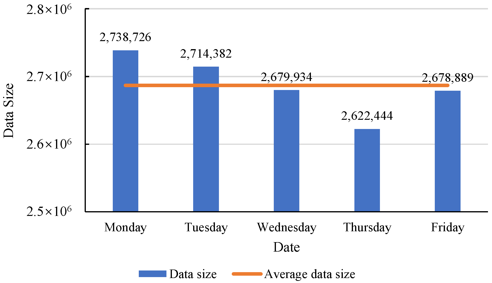
Figure A2.
Cumulative probability of bus speeds within the 100 m buffer zone of the stops.
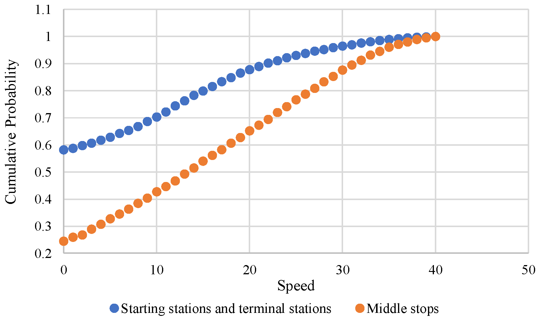
Figure A3.
Sensitivity analysis of speed thresholds at the origin and destination stations.
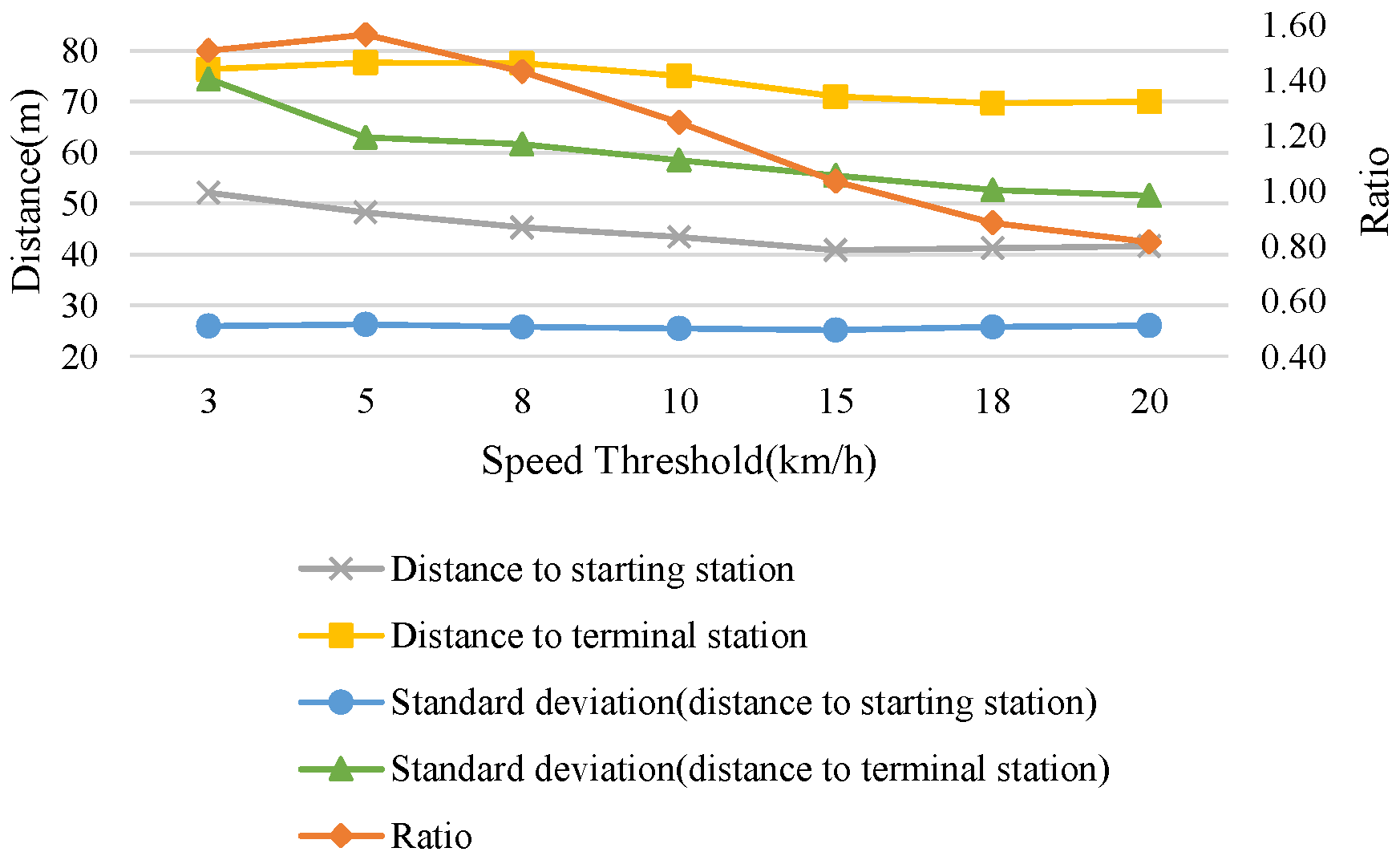
Figure A4.
Sensitivity analysis of the speed threshold at intermediate stops.
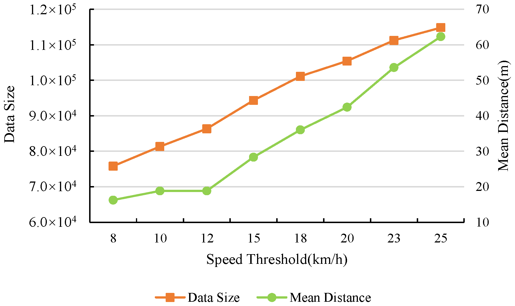
Figure A5.
Error analysis of the completed GPS data of Bus Route 307.
Appendix B
The content of this appendix section presents the ANOVA test results of the clustering coefficients for the static network and DWDN I.
Table A1.
Test of homogeneity of variances.
Table A2.
Robust test for equality of means.
Table A3.
Post hoc tests (partial results).
References
- Gao, B.; Liu, J. Optimizing urban bus network based on spatial matching patterns for sustainable transportation: A case study in Harbin, China. PLoS ONE 2024, 19, e0312803. [Google Scholar] [CrossRef] [Scilit]
- Chen, G.; Wen, G.; Yu, W. A survey of studies on urban public transportation networks based on complex network. J. Nanjing Univ. Inf. Sci. Technol. 2018, 10, 401–408. [Google Scholar] [CrossRef]
- Kozhabek, A.; Chai, W. A multi-scale network-based topological analysis of urban road networks in highly populated cities. Environ. Plan. B-Urban Anal. 2025, 52, 1949–1973. [Google Scholar] [CrossRef] [Scilit]
- Hao, X.; Hu, X.; Zhang, K.; Chen, Q. Assess spatial equity considering the similarity between GIS-based supply and demand maps: A new framework with case study in Beijing. ISPRS Int. J. Geo-Inf. 2025, 14, 157. [Google Scholar] [CrossRef] [Scilit]
- Liu, M.; Zhang, C.; Huang, W.; Wang, M.; Xiao, G. A dynamic network data envelopment analysis cross-efficiency evaluation on the benefits of bus transit services in 33 Chinese cities. Transp. Lett. 2023, 16, 392–404. [Google Scholar] [CrossRef] [Scilit]
- Zhang, H.; Liu, Y.; Shi, B.; Jia, J.; Wang, W.; Zhao, X. Analysis of spatial-temporal characteristics of operations in public transport networks based on multisource data. J. Adv. Transp. 2021, 2021, 6937228. [Google Scholar] [CrossRef] [Scilit]
- Li, H.; Chen, C.; Yuan, Y.; Xia, X.; Huang, Q.; Ye, L.; Huang, Z. Equity analysis of bus network balance from the perspective of spatial morphology and service capability. Sci. Rep. 2025, 15, 2339. [Google Scholar] [CrossRef] [Scilit] [PubMed]
- Wang, Y.; Deng, Y.; Ren, F.; Zhu, R.; Wang, P.; Du, T.; Du, Q. Analysing the spatial configuration of urban bus networks based on the geospatial network analysis method. Cities 2020, 96, 102406. [Google Scholar] [CrossRef] [Scilit]
- Yang, Q.; Zhang, Y.; Zhou, Y. A Review of Complex Network Theory and its application in the resilience of public transportation systems. China J. Highw. Transp. 2022, 35, 215–229. [Google Scholar] [CrossRef]
- Zhen, Y.; Hu, J.; Yang, M.; Zang, R. A review of resilience assessment and recovery strategies for urban multimodal public transportation networks. Urban Transp. China 2025, 23, 25–39. [Google Scholar]
- Feng, J.; Xu, Q.; Li, X.; Yang, Y. Complex network study on urban rail transit systems. J. Transp. Syst. Eng. Inf. Technol. 2017, 17, 242–247. [Google Scholar] [CrossRef]
- Yang, S.; Cao, S.; Yang, C.; Wang, J.; Ye, Y. Review of the application of complex network theory in the field of integrated passenger transport modeling and network evaluation. Sci. Technol. Eng. 2024, 24, 11964–11978. [Google Scholar] [CrossRef]
- Xu, Q.; Zu, Z.; Xu, Z.; Zhang, W.; Zheng, T. Space p-based empirical research on public transport complex networks in 330 cities of China. J. Transp. Syst. Eng. Inf. Technol. 2013, 13, 193–198. [Google Scholar] [CrossRef] [Scilit]
- Tang, Q.; Feng, H.; Li, W. Topology of Changsha public traffic network based on complex network theory. J. Transp. Inf. Saf. 2013, 31, 49–52. [Google Scholar] [CrossRef]
- Di, Z.; Shuai, B.; Zhong, Y. Research on topological properties of public transport network in Chengdu based on complex network. J. Xihua Univ. (Nat. Sci.) 2015, 34, 12–16+22. [Google Scholar] [CrossRef]
- Cao, N.; Cao, H. Exploring the robustness of urban bus network: A case from Southern China. Chin. J. Phys. 2020, 65, 389–397. [Google Scholar] [CrossRef] [Scilit]
- Zhang, D. Analysis of urban public transit network based on complex network. J. Lanzhou Jiaotong Univ. 2014, 33, 120–123+130. [Google Scholar] [CrossRef]
- Pu, H.; Li, Y.; Ma, C. Topology analysis of Lanzhou public transport network based on double-layer complex network theory. Phys. A Stat. Mech. Appl. 2022, 592, 126694. [Google Scholar] [CrossRef] [Scilit]
- Kong, F.; Zhou, F.; Li, X. Characteristic analysis of urban public transport networks based on space-p complex network model. Comp. Sci. 2018, 45, 125–130. [Google Scholar]
- Hu, B.; Pei, Y.; He, N. Modeling and characteristics analysis of bus transport complex network of Harbin. J. Wuhan Univ. Technol. 2017, 39, 20–25. [Google Scholar]
- Jia, G.; Ma, R.; Hu, Z. Urban transit network properties evaluation and optimization based on complex network theory. Sustainability 2019, 11, 2007. [Google Scholar] [CrossRef] [Scilit]
- Háznagy, A.; Fi, I.; London, A.; Németh, T. Complex network analysis of public transportation networks: A comprehensive study. In Proceedings of the 2015 International Conference on Models and Technologies for Intelligent Transportation Systems (MT-ITS), Budapest, Hungary, 3–5 June 2015. [Google Scholar] [CrossRef] [Scilit]
- Regt, R.; Ferber, C.; Holovatch, Y.; Lebovka, M. Public transportation in Great Britain viewed as a complex network. Transp. A Transp. Sci. 2019, 15, 722–748. [Google Scholar] [CrossRef] [Scilit]
- Bona, A.; Rosa, M.; Fonseca, K.; Lüders, R. A reduced model for complex network analysis of public transportation systems. Phys. A Stat. Mech. Appl. 2021, 567, 125715. [Google Scholar] [CrossRef] [Scilit]
- Tran, V.; Cheong, S.; Bui, N. Complex network analysis of the robustness of the Hanoi, Vietnam bus network. J. Syst. Sci. Complex. 2019, 13, 1251–1263. [Google Scholar] [CrossRef] [Scilit]
- Hong, J.; Tamakloe, R.; Lee, S.; Park, D. Exploring the topological characteristics of complex public transportation networks: Focus on variations in both single and integrated systems in the Seoul Metropolitan Area. Sustainability 2019, 11, 5404. [Google Scholar] [CrossRef] [Scilit]
- Shanmukhappa, T.; Ho, W.; Tse, C. Spatial analysis of bus transport networks using network theory. Phys. A Stat. Mech. Appl. 2018, 502, 295–314. [Google Scholar] [CrossRef] [Scilit]
- Abdelaty, H.; Mohamed, M.; Ezzeldin, M.; Wael, E. Quantifying and classifying the robustness of bus transit networks. Transpmetrica A-Transp. Sci. 2020, 16, 1176–1216. [Google Scholar] [CrossRef] [Scilit]
- Horváth, B. Do more people use public transport that is more understandable? In Proceedings of the 4th Cognitive Mobility Conference, Cham, Switzerland, 2–3 October 2025. [Google Scholar] [CrossRef] [Scilit]
- Zhang, X.; Chen, G.; Han, Y.; Gao, M. Modeling and analysis of bus weighted complex network in Qingdao city based on dynamic travel time. Multimed. Tools Appl. 2016, 75, 17553–17572. [Google Scholar] [CrossRef] [Scilit]
- Zhang, X.; Ren, Y.; Huang, B.; Han, Y. Analysis of time-varying characteristics of bus weighted complex network in Qingdao based on boarding passenger volume. Phys. A Stat. Mech. Appl. 2018, 506, 376–394. [Google Scholar] [CrossRef] [Scilit]
- Li, J.; Bai, H.; Wang, S. Analysis method of urban buses dynamic distribution based on complex network. J. Hefei Univ. Technol. (Nat. Sci.) 2022, 45, 1225–1231. [Google Scholar]
- Zhao, S.; Yang, X.; Dai, T. Within-day variation of the complexity of bus passenger flow network based on smart card data. J. Geo-inf. Sci. 2020, 22, 1254–1267. [Google Scholar] [CrossRef]
- Li, X.; Wang, S.; Zhou, L.; Sun, Y.; Zheng, J.; Liu, C.; Zhou, J.; Su, C.; Xu, D. Geospatial analytics of urban bus network evolution based on multi-source spatiotemporal data fusion: A case study of Beijing, China. ISPRS Int. J. Geo-Inf. 2025, 14, 112. [Google Scholar] [CrossRef] [Scilit]
- Perez, Y.; Pereira, F. Effects of Sunday free fare policy in São Paulo bus transportation: A case study through complex network analysis. Case Stud. Transp. Policy 2025, 22, 101595. [Google Scholar] [CrossRef] [Scilit]
- Li, X.; Teng, M.; Jiang, S.; Han, Z.; Gao, C.; Nekorkin, V.; Radeva, P. A dynamic station-line centrality for identifying critical stations in bus-metro networks. Chaos Solitons Fractals 2025, 194, 116102. [Google Scholar] [CrossRef] [Scilit]
- Yang, J.; Chen, Z.; Criado, R.; Zhang, S. A mathematical framework for shortest path length computation in multi-layer networks with inter-edge weighting and dynamic inter-edge weighting: The case of the Beijing bus network, China. Chaos Solitons Fractals 2024, 182, 114825. [Google Scholar] [CrossRef] [Scilit]
- Li, Z.; Tang, J.; Feng, T.; Liu, B.; Cao, J.; Yu, T.; Ji, Y. Investigating urban mobility through multi-source public transportation data: A multiplex network perspective. Appl. Geogr. 2024, 169, 103337. [Google Scholar] [CrossRef] [Scilit]
- Clauset, A.; Shalizi, C.; Newman, M. Power-law distributions in empirical data. SIAM Rev. 2009, 51, 661–703. [Google Scholar] [CrossRef] [Scilit]
- Humphries, M.; Gurney, K. Network ‘Small-World-Ness’: A quantitative method for determining canonical network equivalence. PLoS ONE 2008, 3, e0002051. [Google Scholar] [CrossRef] [Scilit]
- Wiseman, Y. Autonomous vehicles will spur moving budget from railroads to roads. Int. J. Intell. Unmanned Syst. 2024, 12, 19–31. [Google Scholar] [CrossRef] [Scilit]
- Yu, Q.; Yuan, J. TransBigData: A python package for transportation spatio-temporal big data processing, analysis and visualization. J. Open Source Soft. 2022, 7, 4021. [Google Scholar] [CrossRef] [Scilit]
- Wang, C.; Cui, Z.; Du, Z. Repairing of missing bus arrival data based on DBSCAN algorithm and multi-source data. J. Comp. Appl. 2019, 39, 3184–3190. [Google Scholar]
- Telesford, Q.; Joyce, K.; Hayasaka, S.; Burdette, J.; Laurienti, P. The ubiquity of small-world networks. Brain Connect. 2011, 1, 367–375. [Google Scholar] [CrossRef] [Scilit]
- GB/T 51328-2018; Standard for Urban Comprehensive Transport System Planning. China Architecture & Building Press: Beijing, China, 2018.

Disclaimer/Publisher’s Note: The statements, opinions and data contained in all publications are solely those of the individual author(s) and contributor(s) and not of MDPI and/or the editor(s). MDPI and/or the editor(s) disclaim responsibility for any injury to people or property resulting from any ideas, methods, instructions or products referred to in the content. |
© 2026 by the authors. Licensee MDPI, Basel, Switzerland. This article is an open access article distributed under the terms and conditions of the Creative Commons Attribution (CC BY) license.