


Abstract
Networks of fixed, low-cost dose-rate sensors monitor radiological facilities, but the trustworthiness of their reports rests on heuristics: existing trust schemes score nodes by mutual voting or behavioral statistics, which fail against an adversary who falsifies data consistently with the physics the network can observe. This paper presents PRAHARI, a trust management framework in which an unmanned aerial system carrying a calibrated scintillator chain hovers at each node as a mobile metrological anchor. Trust evidence is a statistically principled compatibility test between two uncertainty-quantified measurements with an empirically verified false-alarm rate, feeding a multi-channel Beta reputation engine with wall-clock forgetting, endurance-constrained verification scheduling, and trust-gated dose mapping. Across 9640 paired Monte Carlo trials on a shielded-facility twin with randomized attack classes, PRAHARI is compared against three published network-internal trust methods, a physics-model residual detector, and an uncertainty-blind aerial band. Only aerial-reference evidence discriminates scaling and physics-consistent falsifiers (class AUC 0.80 and 0.75), while network-internal methods stay near chance (0.48 to 0.60), an advantage persisting across facility variants and up to half the adversary’s shielding knowledge, at a false-accusation rate one order of magnitude below every alternative of comparable ranking power. Sensitivity, ablation, reference-bias, and drift studies bound the claims.
1. Introduction
Nuclear processing facilities, storage sites, and radiological emergency zones increasingly rely on networks of fixed, low-cost dose-rate sensors for continuous area monitoring. These networks promise persistent situational awareness at a fraction of the cost of staffed surveys, and they feed decisions with direct safety consequences, among them worker access control, source accountability, and the declaration of high radiation areas. The value of every such decision rests on an assumption that is rarely examined, namely that the numbers arriving at the gateway describe the radiation field that actually exists.
That assumption fails in two distinct ways. Sensors fail as instruments when they drift out of calibration, freeze, fall silent, or grow noisy. Sensors also fail through compromise, when a node reports values chosen by an adversary. The literature on trust management in wireless sensor networks addresses both failure families with a common strategy in which nodes score one another through behavioral statistics, neighborhood voting, and reputation updates [1,2,3,4]. These mechanisms share a structural weakness. All of their evidence originates inside the network being evaluated. An adversary who understands the deployment can therefore fabricate reports that are internally consistent, properly distributed, and mutually corroborating, leaving the network without an independent standard that could expose the fabrication.
The weakness is not hypothetical in the radiological setting. The physical quantity being measured obeys known laws, and an attacker can exploit exactly that. A falsifier that models the source inventory with a simple inverse-square superposition produces reports with correct counting statistics and smooth spatial structure, passing every check the network can run on itself. What such an attacker cannot reproduce is the effect of facility shielding on the true field, because walls, vessels, and partitions imprint a structure that only an independent, calibrated measurement can reveal.
This observation motivates PRAHARI (Physics-grounded Reputation and Assurance via Hovering Aerial Reference for IoT; PRAHARI is Sanskrit for sentinel). The framework assigns the role of trust anchor to an unmanned aerial system (UAS) carrying a calibrated CLYC scintillator measurement chain built from first-principles detector physics with a documented uncertainty budget (Section 4.1). The UAS periodically hovers above each node and produces a traceable reference estimate of the ambient dose equivalent rate at the node position. Trust evidence is then a measurement comparison rather than a vote: a compatibility statistic normalizes the disagreement between the node report and the aerial reference by the combined uncertainty of both, yielding a test with an analytic false-alarm rate that we verify empirically before any detection experiment. Aerial radiological measurement itself is a mature capability [5,6,7,8]. To our knowledge, its use as the evidential basis of a sensor-network trust system is novel. The most closely related concept is the mobile calibration reference in cooperative sensing, exemplified by mobile reference stations used to recalibrate low-cost air-quality networks [9]; PRAHARI differs in that the reference does not correct the fleet but adjudicates it, the comparison is a formal compatibility test with a verified false-alarm rate rather than a regression adjustment, and the setting is adversarial, so the anchor must remain valid while a coherent fraction of the fleet is falsifying rather than merely drifting.
The contributions of this paper are as follows.
First, we present the PRAHARI architecture, which converts trust management from a network-internal voting exercise into a metrological verification task anchored by a mobile calibrated reference (Section 3 and Section 4).
Second, we derive an uncertainty-aware compatibility test as the core trust evidence, including a gradient-adaptive bound on the vertical extrapolation error of the aerial reference and interval logic for detector saturation at facility dose rates. We calibrate the test empirically on 2000 honest-node draws in a shielded-facility digital twin, where the empirical false-alarm rate of 0.0015 is statistically consistent with the analytic value of 0.0027, and the test statistic matches its nominal standard normal form (Section 6.1).
Third, we design a multi-channel Beta reputation engine with forgetting applied on the wall clock rather than per evidence arrival. A temporal analysis of the evidence rates shows that the memory horizon must exceed the verification revisit interval, a requirement that arrival-clock aging violates whenever high-rate weak channels coexist with rare strong ones, and we weight channels by their information content, with passes of checks that adversaries satisfy by design carrying near-zero weight (Section 4.4).
Fourth, we define an eight-class fault and attack taxonomy spanning hard instrument faults and metrological falsification, including a physics-consistent falsifier constructed in the stealthy false-data-injection tradition of the cyber-physical security literature [10,11]. We evaluate it in a tiered manner and characterize detection boundaries with a severity ablation, reporting where detection is analytically guaranteed, where it degrades gracefully, and where it is limited by physics or by operational rates (Section 6.3 and Section 6.4).
Fifth, we formulate verification-flight planning as an orienteering problem under sortie endurance and compare four schedulers, finding performance insensitive to routing policy in the mixed campaign but, against falsification classes, systematically worse under uncertainty-driven priority than under coverage-driven revisits, and we explain why (Section 6.6).
Sixth, we evaluate trust-gated fusion of the facility dose map and report that it yields no benefit at fifty-node density: map accuracy is limited by spatial sampling, and gating itself carries a small, resolvable accuracy penalty, while false accusation carries a map-level penalty that the calibrated test avoids (Section 6.5).
Seventh, we compare PRAHARI against three published network-internal trust methods and a physics-model residual detector under identical scenarios with paired statistics, and we quantify the contribution of each evidence channel, the sensitivity to every trust-engine parameter, the effect of the adversary’s shielding knowledge, and robustness across facility variants and reference-chain bias (Section 6.2, Section 6.3, Section 6.8, Section 6.9, Section 6.10 and Section 6.11).
Eighth, we document the complete simulation framework, an all-MATLAB R2026a (The MathWorks, Inc., Natick, MA, USA) implementation with per-trial manifests, seed-isolated random streams, and bit-identical reproducibility; every figure and statistic in this paper is traceable to an archived campaign artifact.
Throughout, we hold to a strict reporting standard. All results are simulation results on a digital twin and are stated as such. Baselines receive the same engine, the same evidence channels where applicable, and identical random scenarios. Findings that cut against the proposed method, including a small area under the curve (AUC) advantage of an aggressive baseline and a small map-accuracy penalty from trust gating, are reported rather than omitted.
2. Related Work
2.1. Trust Management in Wireless Sensor Networks
Reputation-based trust for sensor networks was established by Ganeriwal et al., whose framework maintains Beta distributions over node behavior and updates them with watchdog observations [2]. The Beta reputation model itself, including the aging of old evidence, originates with Josang and Ismail [3]. A large literature followed, surveyed recently for underwater networks in [4] and evaluated comparatively by Gangwani et al. [1], who benchmark three representative trust models against on-off and bad-mouthing attacks and document how sensitive their performance is to attack pattern. Common to these schemes is that trust evidence derives from the network itself, in the form of packet-forwarding behavior, report consistency among neighbors, and statistical regularity of reported values. Such evidence is effective against crude faults and selfish behavior, and our results confirm this, since a purely network-internal ensemble detects hard faults perfectly in our experiments. It is structurally blind, however, to an adversary who fabricates internally consistent data, a gap our physics-consistent falsifier makes concrete.
2.2. UAS in Sensor Networks and Radiological Monitoring
UAS have been integrated into sensor networks primarily as communication and logistics assets such as mobile sinks that collect data from energy-constrained nodes, relays that extend coverage, and mobile chargers [12,13]. In parallel, aerial radiological measurement has matured from manned survey aircraft to multirotor and fixed-wing UAS platforms carrying scintillator and semiconductor spectrometers, with deployments ranging from the Fukushima response [7] to facility and legacy-site surveys [5,6,8]. These two lines of work meet in PRAHARI in a role that neither has assigned to the UAS before. The aircraft is neither a data mule nor a mapper but a mobile calibration standard whose measurements adjudicate the honesty of the ground network. The measurement chain we carry, a CLYC scintillator with pulse-shape discrimination [14], is specified in Section 4.1 entirely from published detector physics and metrology standards [15,16,17].
2.3. Physics-Based Integrity Verification
In cyber-physical systems more broadly, the insight that falsified data must be checked against physical models has produced a substantial body of work, from false data injection analysis in power grids [10] to the survey of physics-based attack detection by Giraldo et al. [11]. Most of this work checks reported data against a model of the process. PRAHARI differs in checking reported data against an independent measurement of the process, with both sides carrying explicit uncertainty budgets in the sense of the Guide to the Expression of Uncertainty in Measurement (GUM) [15]. The distinction matters against our strongest adversary, whose reports satisfy plausible process models by construction and are exposed only where the true field, shaped by shielding the attacker cannot see, departs from any smooth model. Our own prior work applied deep sequence models to detect anomalous drone trajectories near protected facilities [18]; the present paper addresses a complementary integrity problem in the same setting, using the aerial platform to protect the ground network.
3. System and Threat Model
3.1. Facilities, Nodes, and Gateway
We consider a shielded processing facility instrumented with N fixed dose-rate nodes at working height, reporting over a low-power wide-area uplink to a gateway that maintains trust state and a fused facility dose map. The ground truth environment in all experiments is a digital twin of a canyon-style processing facility (see Figure 1), comprising a 27 by 17 by 8.5-m hall with twelve processing cells, interior partitions, four point sources and a uniform contamination level in each cell (Table A8), in which the point-source field is computed by ray tracing with Beer-Lambert attenuation, a linear buildup factor B = 1 + 0.12 μx (the thin-shield simplification of the Taylor form), finite-height walls, steel process vessels, single-scatter ceiling skyshine, and floor albedo. The resulting field spans roughly 0.003 to 14 mSv/h at node height (up to 318 mSv/h in the volume immediately around the sources), converted from exposure-rate units with the coefficients of ICRU Report 47 and ICRP Publication 74 [16].
Figure 1.
Plan view of the facility digital twin at node mounting height, showing the true H*(10) dose-rate field on a log scale with the eleven concrete wall segments, the four point sources, the fifty node positions of campaign seed 1, and the gateway overlaid. The 30 cm partitions imprint the order-of-magnitude dose discontinuities that the wall-blind T8 falsifier cannot reproduce.
Each node is a GM-class area monitor with a dose-rate sensitivity of 2000 counts per second per mSv/h, a 100 microsecond non-paralyzable dead time [17], and a background of 0.5 counts per second, parameterized after a commercial energy-compensated tube [19]. Every node carries a deployment-fixed unit-to-unit calibration bias drawn from a zero-mean normal distribution, truncated at 2.5 standard deviations, whose standard deviation is the 15 percent Type B response allowance of its instrument class [20]; simulating this bias is essential, because it is precisely the physical quantity the systematic term of the uncertainty budget accounts for. Nodes report every 300 s after a 60 s counting dwell. The uplink follows a log-distance path-loss model with lognormal shadowing using in-building obstructed parameters [21] and a link budget after a commercial LoRa-class transceiver [22]. Node energy accounting covers sensing, transmission, and sleep, with network lifetime tracked by the first-node-death convention [23].
3.2. Aerial Reference
A multirotor UAS carries a calibrated CLYC measurement chain: a one-inch Cs2LiYCl6:Ce scintillator [14] with 4 microsecond dead time and 5 counts per second intrinsic background, whose dose-rate sensitivity we derive at run time from the crystal geometry, the total intrinsic efficiency at 662 keV, and the ICRP-74 fluence-to-dose coefficient [16], rather than assuming it. The calibration-side systematic budget combines mass attenuation, geometry, dead time, and conversion-coefficient components in quadrature following the GUM [15]. The platform flies four sorties per day with 15 min of usable endurance each, transits at 3 m/s, and dwells 30 s at each of two vertical standoffs above a visited node.
3.3. Adversary and Fault Model
The threat scenario assumes that a fraction of nodes is compromised or faulty for the full mission. We define eight classes in two tiers. Tier 1 comprises hard instrument faults: T2 freezes the entire report packet; T3 falls silent, either permanently or with a configurable duty; T4 produces overdispersed counts through a mean-preserving negative binomial process. Tier 2 comprises metrological falsification, in which the node fabricates internally consistent packets whose counts, dose, and stated uncertainty all derive from a falsified rate passed through the same counting model an honest node uses: T1 applies a slow multiplicative calibration drift on top of the unit’s deployment bias; T5 shifts the reported dose by a constant offset; T6 scales it; T7 lies intermittently, applying the T5 payload on a random fraction of epochs. T8, the strongest adversary, reports from a wall-blind physical model of the facility, an inverse-square superposition over the true source inventory plus background. T8 nodes share this model, so colluding falsifiers are mutually coherent in space, their counts are properly Poisson, and their reports respect source proximity structure. The threat model grants the T8 adversary the source inventory but not the shielding geometry, which is realistic for an insider with process knowledge and is exactly the asymmetry an independent calibrated measurement can exploit. Partial shielding knowledge, obtained, for example, from facility drawings or inferred by correlating fixed-node reports over time, would interpolate the adversary between the wall-blind model studied here and an oracle falsifier. The headline detection power should therefore be read as the result against a fully wall-blind adversary, and Section 6.10 sweeps that knowledge from wall-blind to oracle, showing that the advantage of the reference persists up to about half knowledge and is lost near three quarters. Ground-truth labels exist only for scoring; no runtime component reads them except an oracle baseline that defines the achievable headroom.
4. PRAHARI Framework
4.1. Measurement Chain
Figure 2 summarizes the architecture developed in this section. Both detector classes share one forward and inverse measurement chain, differing only in calibration constants. Forward, the true ambient dose rate at the detector position maps to a true count rate through the sensitivity and any gain factor, the non-paralyzable dead time compresses it to an observed rate [17], and counts over the dwell are drawn from an exact Poisson process, using the Knuth method at low rates and the transformed-rejection method of Hormann at high rates [24], so that the dispersion properties on which downstream tests rely are exact rather than approximate. Inverse, the instrument recovers the true rate through the dead-time inversion with a guard near the 1/tau asymptote, subtracts background, and converts to dose rate; statistical uncertainty propagates through the inversion by first-order sensitivity, and the systematic allowance is applied on the recovery side, both per the GUM [15]. When the dead-time inversion reaches its guard, the measurement is flagged over-range and its value becomes a certified lower bound at the largest recoverable dose, about 45 mSv/h for the GM node and 15 mSv/h for the CLYC. This is genuine physics of high-sensitivity counters at facility dose rates and shapes both the compatibility test and the fusion below.
Figure 2.
PRAHARI system architecture. Fixed GM dose-rate nodes report over a low-power uplink while a UAS carrying a calibrated CLYC measurement chain hovers at two standoffs above scheduled nodes and extrapolates a traceable reference to the node position. The uncertainty-normalized compatibility test converts each verification into calibrated trust evidence, which joins three network-internal channels in a Beta trust engine with wall-clock forgetting; trust gates the fused facility dose map, and trust state drives the next verification schedule. Blue markers denote honest nodes and the red marker a compromised node; dashed blue arrows show report uplinks and verification sorties.
4.2. Aerial Reference at a Node
The UAS cannot occupy a node’s mounting point, so it measures at two vertical standoffs s1 = 1 m and s2 = 2 m above the node and extrapolates log-linearly to the node height using only its own two measurements. The Type A uncertainty of the extrapolated value follows from the two measurement uncertainties through the extrapolation weights. The model error of the log-linear step is bounded adaptively: for the worst local geometry, a dominant point source directly below the node at depth d, the exact extrapolation error divided by the observed difference between the two standoff readings is at most 0.9 for all d of at least one meter, so we set the model term to a small floor plus 0.9 times the observed log difference. The bound derives from geometry, tightens automatically where the field is flat, and is honest where gradients are steep; its adequacy is exactly what the calibration experiment of Section 6.1 verifies. The CLYC calibration systematic is common to both standoff measurements and is carried once. If either standoff measurement is over-range, the reference degrades to a certified lower bound.
4.3. The Compatibility Test
Trust evidence at a verification is the normalized disagreement between the node report and the aerial reference, computed in log-dose space because the field spans decades and both uncertainty budgets are closer to relative than absolute. Statistic E divides the difference of log doses by the combined uncertainty, which sums in quadrature the node’s statistical and systematic terms and the reference’s extrapolation and systematic terms. Under the null hypothesis of an honest node with correct budgets, E follows a standard normal distribution to first order, so a threshold of k standard deviations carries the analytic false-alarm rate 2(1 − Φ(k)); we use k = 3, for 0.0027. When one side is over-range, the test degrades to one-sided interval logic. A saturated node is compatible if the reference confirms at least its measurement ceiling; a finite node against a saturated reference is compatible only if it claims at least the reference’s certified bound; two saturated instruments are mutually consistent. This prevents false accusations of honest instruments at hot cells while still catching suppression attacks that report low where the reference pegs high. Verification power is reduced in over-range regions; a scope limit we state rather than hide.
4.4. Trust Engine
Per-node trust is a Beta posterior over honest reporting, updated by four evidence channels. The first is the compatibility outcome of each aerial verification. The second is a spatial channel comparing each report against a trust-weighted prediction from neighbors within 8 m. The third is a node-local dispersion self-test applying an exact chi-square statistic to the sub-window counts of each report, together with a cross-epoch repetition check. The fourth is an availability channel that records expected-but-missing reports. Forgetting toward the prior follows the aging concept of [3] but is applied once per report epoch on the wall clock, with a two-day memory constant. The distinction is not cosmetic: per-arrival aging couples the memory horizon to the evidence arrival rate. With roughly three internal arrivals per epoch, it gave the trust state a half-life near one hour, structurally erasing aerial evidence that arrives about once per 1.25 days per node. The design requirement is that the memory horizon exceed the verification revisit interval, and the two-day constant satisfies it with margin while still bounding how much an intermittent liar can bank.
Channel weights follow information content. A compatibility failure is a calibrated event with a 0.27 percent false-alarm rate and carries weight 5. A pass certifies only local, momentary consistency and carries weight 1: an intermittent liar passes on its honest epochs, and the wall-blind falsifier passes wherever its model happens to be right. A dispersion or repetition alarm at 0.001 level carries weight 2. Passes of the self and availability checks carry near-zero weight 0.01, because every falsification class passes them by design, which makes their pass log-likelihood ratio essentially zero: presence and internal consistency must not accumulate honesty credit. The spatial channel, an uncalibrated heuristic, carries symmetric soft weight 0.05; Section 6.8 shows that this weight sits at the edge of a cliff, and that lowering it improves the detection of coherent falsifiers. A node whose trust mean falls below 0.30 is flagged. All weights were fixed at design time on a synthetic development world, a 30 by 20 by 8 m analytic layout with three randomized point sources and a single idealized 30 cm concrete partition. That world is reserved for unit tests and end-to-end checks and is never used for reported results. Weights were assigned analytically from the calibrated evidential value of each channel outcome rather than by empirical search, with failure and alarm weights scaled to their analytic false-alarm rates and pass weights held at the near-zero log-likelihood ratios argued above. They were exercised end-to-end against representative fault and falsification classes on that world, and no weight was revisited after any facility-twin result was observed. Every baseline that uses a channel uses it with identical weights.
4.5. Verification Scheduling
Each sortie selects and orders nodes to verify under the endurance budget, with travel at transit speed and a fixed per-visit cost of two dwells plus approach overhead. We cast this as an orienteering problem [25]: each node carries a priority equal to its Beta variance times a staleness factor times a criticality factor derived from the current fused dose estimate at the node, never from ground truth. We implement four policies with identical budgets: random insertion, round robin, greedy insertion by priority per marginal time, and simulated annealing [26] over insert, remove, and swap moves starting from the greedy route. Section 6.6 reports that, against falsification classes, the variance-driven priority underperforms systematic coverage, and explains why.
4.6. Trust-Gated Fusion
The gateway maintains a facility dose map by inverse-distance weighting of the latest reports in log space on a 2 m grid, with each report weighted by a soft trust gate, its inverse relative variance, and inverse distance. The combiner is deliberately standard, since the object of study is what trust weighting contributes, not the mapper. Over-range reports enter as censored observations at their certified bound, which is the conservative behavior a protection map should have and is what keeps regions hotter than the instruments’ range correctly classified above action levels. Map quality is scored against the true field slice on covered cells by log-domain RMSE and by detection of high radiation areas at the regulatory action level of 1 mSv/h defined in 10 CFR 20.1003 [27].
5. Experimental Design
All experiments run on the facility twin with N = 50 nodes, three simulated days, four sorties per day, and, unless stated otherwise, fifty independent seeds per configuration. A digital twin is used by necessity rather than convenience: evaluating trust management requires ground-truth knowledge of the radiation field and of which nodes are falsifying, and no such dataset exists publicly for an instrumented nuclear facility, since layouts, shielding geometry, and source inventories are security-sensitive, while open environmental radiation streams contain neither attacks nor ground truth. The twin is therefore constructed entirely from published physics and metrology, with every constant carrying a citation, and Section 6.1 verifies empirically that the simulated measurement chain reproduces the analytic behavior its uncertainty budget predicts. The compromised count is round(fraction × N), half away from zero: 3, 5, 10, and 15 of fifty nodes, so the nominal fraction 0.05 is an effective 0.06 and the others are exact. Compromised nodes are drawn uniformly at random from fifty, and each compromised node draws its fault or attack class uniformly at random from the eight classes of Section 3, both on the per-trial world-and-attack stream. The class composition is therefore statistically identical at every compromise fraction and identical across trust modes for a given seed. Table 1 reports the realized composition. The submitted version of this study assigned classes cyclically in draw order, which made composition depend on the fraction: at 0.05 only T1 to T3 were present, at 0.10 only T1 to T5, and T8 had exactly one node per trial at 0.20 and 0.30. All results reported here are from the corrected campaign. Random streams follow a strict discipline: callers seed, library code never seeds, and each trial derives isolated streams for the world and attack draw versus runtime stochastics, so that all trust modes face identical scenarios under common random numbers. Same-seed re-execution reproduces every trial bit for bit, a property we exercised across three full campaign repetitions, and extending the seed list appends trials without perturbing existing ones.
Table 1.
Realized attack-class composition of the trust campaign (PRAHARI mode; identical for every mode at the same seed): mean number of nodes of each class per trial, and in parentheses the number of the fifty trials in which the class is present. Row totals are 3, 5, 10, and 15 nodes; the nominal fraction 0.05 is an effective 0.06 (three of fifty nodes).
We compare eight modes under identical scenarios. PRAHARI uses all channels. A naive variant replaces the compatibility test with an uncertainty-blind fixed band that accepts a node if its report lies within 20 percent of the reference value, representing what a heuristic scheme without metrology can do with the same aircraft; Section 6.8 sweeps the band from 10 to 40 percent. A voting mode uses all network-internal channels with PRAHARI weights but no aerial evidence, so the difference between PRAHARI and voting isolates exactly the reference channel. Three further network-internal baselines are adaptations of published methods to the dose-report setting, fed the same evidence events as voting. The first, btres, follows the Beta-based Trust and Reputation Evaluation System [28], one of the three frameworks benchmarked in [1]: a Beta posterior over honest behavior updated from binary observations (report delivered, neighbor agreement within two sigma, self-test not alarmed) with symmetric unit pseudo-counts, aging applied at every evidence arrival with factor 0.98, and a punishment weight that grows with consecutive misbehavior, capped at three. The second, ltmbe, follows the Lightweight Trust Management scheme based on Bayesian and Entropy [29], also benchmarked in [1]: the same direct Beta trust, plus a recommendation trust from neighbors weighted by the recommenders’ own trust, fused with the weight one minus the normalized binary entropy of the direct trust mean so that confident direct evidence dominates and uncertain direct evidence defers to recommendations. The third, cusum, is the physics-model integrity check of the residual-based family surveyed in [11]: a one-sided cumulative sum [30] on the standardized residual between each report and a smooth leave-one-out inverse-distance model of its neighbors, with slack 1.0 and decision threshold 8, mapped to a trust score so that the threshold coincides with the flag level. Neither the packet-forwarding watchdog of the original Beta-reputation schemes nor multi-hop routing exists in this single-hop network, and we state that these are style adaptations rather than verbatim reimplementation; their update rules are given in Appendix A. A no-trust mode leaves the engine inert. An oracle mode reads ground-truth labels and bounds achievable performance. Metrics cover node-level detection (AUC by the rank statistic of [31], flagged fraction, false-accusation rate, flag precision, and time to detection), map quality (log RMSE and high-radiation-area F1), network lifetime, and UAS effort. Because all modes face identical scenarios under common random numbers, per-seed observations are paired. Statistical analysis therefore uses a Friedman omnibus [32] over modes with seeds as blocks, per metric and compromise fraction, followed by Wilcoxon signed-rank tests [33] of PRAHARI against each baseline on the per-seed differences, Bonferroni-corrected over the seven key pairs, with the paired effect size dz (mean difference over its standard deviation), a bootstrap 95 percent percentile interval of the mean paired difference from 2000 resamples, and, for continuity with the unpaired protocol of the submitted version, Cohen’s d and Cliff’s delta [34]. Compromise fractions span from 0 to 0.30; the zero-compromise condition supplies the clean-network false-accusation exposures and is omitted from AUC figures because AUC is undefined without positive instances. Figures plot means with standard-deviation bars over seeds, except that rate-valued figures use bootstrap 95 percent percentile intervals of the mean, which respect the unit-interval bounds of a rate; the running text reports medians of the same per-seed distributions, which is why the two can differ slightly at this sample size. The archived count decomposes as 2000 trust trials (eight trust modes, five compromise fractions, fifty seeds), 200 scheduler trials (four schedulers, fifty seeds) plus 200 on falsification classes only, 1200 severity trials (six classes, four levels, fifty seeds), 3100 trust-parameter and spatial-weight sensitivity trials, 600 evidence-channel ablation trials, 500 adversary-knowledge trials, 700 reference-bias trials, 600 drift-remedy trials, and 540 facility-variation trials (nine variants, three modes, twenty seeds), giving the 9640 archived Monte Carlo trials cited throughout. The complete implementation, per-trial artifacts, run manifests, and analysis scripts are retained as archived study records and are available as described in the Data Availability Statement.
6. Results
6.1. Calibration of the Compatibility Test
Before any detection experiment, we verify that the compatibility statistic behaves as its uncertainty budget predicts. Over 2000 honest-node draws at random facility positions, each with an independently drawn unit calibration bias, E is empirically distributed with mean 0.023 and standard deviation 0.902 against the nominal standard normal, and the empirical false-alarm rate at k = 3 is 0.0015 with a 95 percent confidence interval [0.0000, 0.0032], statistically consistent with the analytic 0.0027 and slightly conservative, as expected from the truncated bias draw. Single-flight detection power at the same operating point is 0.969 against T6, 0.817 against T8, and 0.319 against T5, the last correctly reflecting that a fixed offset of 0.5 mSv/h is proportionally invisible at high dose rates and conspicuous near background. Table 2 summarizes.
Table 2.
Compatibility test calibration on the facility twin (2000 independent honest node-verification draws, k = 3).
6.2. Node Integrity Across Compromise Fractions
Figure 3 shows detection AUC versus compromise fraction. PRAHARI separates decisively from the no-trust floor at every fraction, with median AUC 0.855 at a compromise fraction of 0.05, 0.860 and 0.811 at the intermediate fractions, and 0.836 at 0.30, against 0.500 for no trust; the signed-rank test saturates at its fifty-seed floor (corrected p = 5.3 × 10⁻⁹) with paired dz between 2.2 and 4.7 and Cliff’s delta between 0.96 and 1.00. PRAHARI tracks the oracle bound of 1.000 within 0.17 to 0.20 mean AUC (0.14 to 0.19 on medians). Against network-internal voting the advantage is present at every fraction and grows with compromise: median 0.855 versus 0.826 at 0.05 (corrected p = 0.0015), 0.860 versus 0.798 at 0.10 (p = 2.7 × 10⁻⁵), 0.811 versus 0.769 at 0.20 (p = 6.7 × 10⁻⁷, dz = 1.06), and 0.836 versus 0.773 at 0.30 (p = 2.1 × 10⁻⁸, dz = 1.16). The three published network-internal baselines fall between voting and PRAHARI: btres 0.823, 0.816, 0.769, 0.779; ltmbe 0.837, 0.813, 0.782, 0.792; cusum 0.830, 0.792, 0.757, 0.750 (medians), with PRAHARI significantly better than each at 0.20 and 0.30 (corrected p between 0.04 and 2 × 10⁻⁸) and better than cusum at every fraction. Against the uncertainty-blind band, PRAHARI is statistically indistinguishable at every fraction (medians 0.894, 0.836, 0.814, 0.826 for the band; corrected p = 1 throughout, dz between −0.13 and −0.30): the two tests have the same ranking power, and the difference between them lies entirely on the false-accusation axis.
Figure 3.
Node detection AUC versus compromised fraction for all eight modes (mean and standard deviation over fifty seeds). PRAHARI separates from the no-trust floor at every fraction, tracks the oracle bound, exceeds every network-internal method, and is statistically indistinguishable from the uncertainty-blind band.
The decisive separation appears on the false-accusation axis (Figure 4) and its operator-facing summary, flag precision (Figure 5). The PRAHARI median false-accusation rate is zero at every fraction; across all 2500 honest-node exposures in clean networks over fifty seeds, four honest nodes were ever flagged, 0.16 percent, consistent with the calibrated alpha compounded over the mission. Every alternative pays more. The uncertainty-blind band maintains a standing false-accusation rate of 2.8 percent of the healthy fleet with zero attackers present, because a fixed agreement band cannot accommodate the legitimate unit-to-unit calibration spread that the GUM budget absorbs by construction; ltmbe accuses 2.0 percent and voting 1.5 percent, because neighbor disagreement at shielding discontinuities is treated as evidence of dishonesty; and cusum accuses 33 percent, because a smooth field model is simply wrong for honest nodes on the far side of a partition, which is the physics argument of this paper in a single number. Only btres matches PRAHARI’s clean-network rate, and it does so because its symmetric unit pseudo-counts never accumulate enough distrust to cross the flag threshold, which is also why it cannot see T6 or T8 (Section 6.3). The differences are significant at every fraction: paired signed-rank corrected p against the blind band is 4.2 × 10⁻⁷, 3.6 × 10⁻⁵, 4.1 × 10⁻⁴ and 3.4 × 10⁻³ at fractions 0.05 to 0.30, against voting 2.2 × 10⁻³ to 2.7 × 10⁻², against ltmbe 3.8 × 10⁻⁵ to 6.8 × 10⁻³, and against cusum below 10−8 throughout. Precision follows: at a fraction of 0.05 the PRAHARI median is 1.000 against 0.500 for the blind band (paired p = 6.7 × 10⁻⁶, dz = 1.62), 0.333 for ltmbe and 0.154 for cusum; at 0.10, 1.000 against 0.750 (p = 1.1 × 10⁻⁴); at 0.20 and 0.30 the medians converge to 1.000 but the mean paired advantage over the blind band remains 0.10 and 0.04 (p = 9.0 × 10⁻⁴ and 3.4 × 10⁻³).
Figure 4.
False-accusation rate versus compromised fraction, including the zero-compromise clean network, for all eight modes. The physics-model residual detector (cusum) accuses 15 to 33 percent of healthy instruments; the uncertainty-blind band and the Beta-reputation baselines accuse 1 to 3 percent; the PRAHARI median is zero everywhere. Points are seed means with standard-deviation bars.
Figure 5.
Flag precision, true positives over all flags, for the six modes that raise flags. PRAHARI holds from 0.97 to 1.00 at all fractions; the uncertainty-blind band ranges from 0.45 to 0.96, ltmbe from 0.32 to 0.86, and cusum from 0.10 to 0.66. Every false flag dispatches maintenance to a certified instrument.
We state the resulting trade plainly, and we correct a claim in the submitted version. The blind band’s ranking power is not lower than the calibrated test’s; the two are statistically indistinguishable, and the band’s raw AUC is marginally higher at every fraction because it accepts more honest-node accusations. Sweeping its tolerance from 10 to 40 percent (Section 6.8) raises its AUC from 0.784 to 0.825 while its clean-network false-accusation rate falls from 4.8 to 1.2 percent; no tolerance in the tested range of 0.10 to 0.40 reaches the 0.16 percent of the calibrated test, so no matched false-alarm operating point was identified within that range. We do not claim that none exists: the false-accusation rate of the band is still falling at 0.40, and a wider band may reach it. We therefore withdraw the statement that the calibrated test dominates at matched cost. What the uncertainty budget buys is precision, not ranking: an order of magnitude fewer wrongful flags at the same ranking power, and, as Section 6.5 shows, a map-level benefit that follows directly from not gating honest instruments out of the fused map. In a licensed facility, where every flag dispatches maintenance to a certified instrument and a system that cries wolf in a clean network is switched off before an attack arrives, that is the binding constraint.
6.3. Per-Class Detection: A Tiered Taxonomy
We present per-class results in two tiers because they answer two different questions. For the hard faults of Tier 1, detection is perfect, with AUC 1.000 and zero variance at a compromise fraction of 0.20, and perfection here is the analytically expected outcome rather than an empirical surprise. Permanent dropout is deterministically visible to the availability channel under a link budget with roughly 30 dB of margin at maximum range. A frozen data path repeats a bit-identical sub-count vector whose probability under honest Poisson counting is on the order of 10−13 per epoch, so the repetition check fires with certainty by the second report. Fivefold overdispersion violates the exact chi-square dispersion statistic at every epoch. These classes are included for taxonomy completeness and because deployed systems must handle them; their detection requires only standard telemetry hygiene, every evaluated scheme detects them equally, and they are not the contribution.
Tier 2 is where the aerial reference earns its numbers, and Table 3, whose PRAHARI row is plotted in Figure 6, now tests the central claim directly. T6 and T8 are the two classes that satisfy every network-internal check by construction: a scaled report is still Poisson, still repeats nothing, still arrives on time, and a coherent group of falsifiers agrees with itself. On these two classes every network-internal method sits at or near chance, voting at 0.585 and 0.585, btres at 0.499 and 0.477, ltmbe at 0.546 and 0.513, cusum at 0.577 and 0.597, while PRAHARI reaches 0.804 and 0.754 (paired corrected p between 5 × 10⁻⁷ and 3 × 10⁻³ against each). At a fraction of 0.30, the ordering is unchanged: T6 0.846 and T8 0.738 against 0.51 to 0.63 for the four network-internal methods. The blind band, which also carries the aerial reference, is close on T8 (0.722, not significant) and behind on T6 (0.767, p = 2 × 10⁻⁴). The table is equally direct about where PRAHARI is not the best method. On the intermittent liar T7, btres and ltmbe reach 0.78 and 0.81 against PRAHARI’s 0.58 (p < 4 × 10⁻³), and on the offset falsifier T5 they reach 0.89 and 0.90 against 0.82 (p < 2 × 10⁻³): their punishment for consecutive misbehavior accumulates the neighbor disagreements that PRAHARI’s soft spatial evidence averages away. On T1, the blind band is marginally better (0.558 against 0.474, p = 4.5 × 10⁻³), a consequence of its wider acceptance of drifting honest units, and every method is near chance for the reason Section 6.4 quantifies. The contribution of the aerial reference is therefore specific: aerial-reference evidence, whether scored by the calibrated test or by the blind band, is the only source that discriminates falsification that leaves no network-internal footprint, and a punishment term of the kind the Beta-reputation baselines use is an obvious addition for the classes that do leave one. Median time to detection of flagged nodes is 0.2 h, so hard faults are isolated within the first report epochs, at a UAS cost of 2.98 flight hours per three-day mission.
Table 3.
Per-class detection AUC (class versus honest) for every trust mode at a compromise fraction of 0.20, mean and standard deviation over the seeds in which the class is present (n in the last row). Paired signed-rank p-values are PRAHARI against the named baseline, Bonferroni-corrected over five baselines; bold marks p < 0.05 in PRAHARI’s favor, italic marks p < 0.05 against PRAHARI.
Figure 6.
Per-class detection AUC, class versus honest, for PRAHARI at a compromise fraction of 0.20 (Table 3 gives all modes).
6.4. Detection Boundaries: Severity Ablation
Reporting a single operating point per class invites the question every reviewer should ask: where does detection break? We answer with a severity ablation, one class active per trial with five compromised nodes among 45 honest, each class swept across four levels from subtle to severe, with fifty seeds per cell, 1200 trials in total, with the headline parameterizations marked in Figure 7 and the values listed in Table 4; each cell reports the mean AUC with a bootstrap 95 percent confidence interval over seeds. Nothing in the headline campaign was altered; this experiment adds the boundary characterization.
Figure 7.
Detection boundaries: PRAHARI detection AUC versus attack severity, one panel per class, with the headline operating point starred and the chance line dotted (mean and standard deviation over fifty seeds; Table 4 gives bootstrap 95 percent confidence intervals). T2 is absent by design, as explained in the text: replaying the last honest value has no severity axis in a static field.
Table 4.
Detection AUC versus attack severity (mean over fifty seeds with bootstrap 95 percent confidence interval in brackets; headline level starred). Each class lists the swept parameter values in its first row and the resulting AUC in its second (* Headline level).
The falsification classes show the expected monotone boundaries, now with intervals narrow enough to place them. T6 is statistically invisible at scales of 0.9 and 0.7, where a 10 to 30 percent suppression sits inside the combined honest budget and AUC at chance is the correct metrological verdict, and detectable from a scale of 0.5 (0.676 [0.636, 0.717]) to 0.3 (0.749 [0.717, 0.782]). T5 rises with payload from 0.614 to 0.831, its residual spread reflecting dose dependence. T7 climbs with lying duty from 0.514 at 5 percent to 0.709 at 50 percent: an attacker can trade impact for stealth, and the wall-clock memory bounds how much lying fits undetected inside one window. T3 exhibits a sharp availability knee: 5 percent packet loss is near-indistinguishable from residual shadowing loss, 20 percent loss is almost fully separable with flags on 52 percent of faulty nodes, and half loss upward is deterministic.
Two boundaries require explicit comment. T4 remains at 1.000 across the sweep: the exact dispersion test applied at every one of 864 report epochs accumulates power far beyond its single-window sensitivity. T1 is the mirror image, at chance for every drift rate up to 10 percent per day and only 0.567 [0.530, 0.603] at 25 percent per day. The reason is a rate mismatch rather than a test failure: a drifting node becomes incompatible only after its accumulated gain exits the response allowance, near day 2.2 at the highest rate, leaving at most a fraction of the mission’s sparse per-node visits, about 0.8 per day, to observe the violation. Section 6.11 tests the two operational remedies. T2 is deliberately absent from the sweep: the subtle variant, replaying the last honest value re-sampled through the counting model, is epistemically harmless in a static field because the replayed value remains correct, and it becomes a T5-class discrepancy only when the field changes. False accusations across the 1200 severity trials remained at the calibrated alpha.
6.5. Map-Level Fusion: No Benefit at Fifty-Node Density
The trust-gated facility map (Figure 8) shows no map-level benefit from calibrated trust relative to no gating, and a map-level penalty from false accusations. For high-radiation-area F1 at the action level [27], PRAHARI is statistically indistinguishable from the unweighted and oracle-gated maps at every fraction (corrected p between 0.37 and 1), while it exceeds the blind band by 0.08 to 0.09 (p between 1 × 10⁻⁵ and 7 × 10⁻⁵), voting by 0.02 to 0.04 (p between 3 × 10⁻³ and 0.17), and cusum by 0.05 to 0.11 (p below 3 × 10⁻³). For grid-average log RMSE, trust gating carries a small but resolvable penalty: the PRAHARI median exceeds the unweighted map by 0.03 to 0.05 log10 units at every fraction (p below 4 × 10⁻⁷), and the oracle map moves in the same direction, so the penalty is a property of gating itself rather than of trust estimation error. Two structural facts explain this outcome. First, absolute map accuracy is limited by interpolation: with fifty nodes sampling a facility whose 30 cm partitions create order-of-magnitude dose discontinuities, the log RMSE floor near 0.65 is set by spatial sampling rather than sensor integrity, and the oracle-gated and unweighted maps are statistically identical in clean networks, proving the limit is geometric. Second, trust gating trades local coverage for integrity: excluding a distrusted node removes its sometimes partially informative local sample. The F1 ordering follows from the second fact. Every false accusation gates an honest instrument out of the map, so the methods with the highest clean-network false-accusation rates produce the worst high-radiation-area maps, and the calibrated test’s precision is what keeps PRAHARI at the unweighted level. The facility-variation study of Section 6.10 finds no density at which gating turns into a net map benefit between 25 and 100 nodes. We conclude that the payoff of calibrated trust is node-level, and that its map-level role is to avoid the damage that heuristic gating does.
Figure 8.
High-radiation-area detection F1 at the 1 mSv/h action level of 10 CFR 20.1003, versus compromised fraction, for the trust-weighted (PRAHARI), voting-weighted, unweighted and oracle-trust maps (mean and standard deviation over fifty seeds). PRAHARI is statistically indistinguishable from the unweighted and oracle-trust maps at every fraction; at fifty-node density the metric is limited by spatial sampling.
6.6. Scheduler Comparison
Across fifty seeds at a compromise fraction of 0.20 (Figure 9), mean detection AUC is 0.810 for random routing, 0.813 for round robin, 0.803 for greedy insertion, and 0.807 for simulated annealing: in the mixed campaign, verification value is insensitive to routing policy, with all four schedulers within 0.01 AUC and an identical median time to detection of 0.2 h, dominated by the fault classes the epoch channels catch regardless of routing. This null result hides a negative one. Restricting the compromised population to the falsification classes T5, T6, and T8, the only classes for which the aerial visit matters, and repeating the study with 200 trials, round robin reaches 0.834 and random routing 0.812, while greedy insertion and simulated annealing fall to 0.772 and 0.766; greedy is below round robin on 44 of 50 paired seeds (mean difference −0.062) and its median time to detection doubles from 6.1 to 12.1 h. The mechanism is the same one that defeats the network-internal channels. The priority of Section 4.5 is the Beta variance of the node, and a coherent falsifier keeps passing every epoch check, so its trust posterior sharpens around a high mean, its variance shrinks, and the uncertainty-driven scheduler stops visiting exactly the nodes that only the aerial reference can catch. Systematic coverage has no such blind spot. We therefore withdraw the preference for priority-driven scheduling expressed in the submitted version, recommend round-robin coverage as the default policy, and identify a falsification-aware priority, weighing by time since the last aerial verification rather than by trust variance, as the obvious next step. The finding also cleanly separates PRAHARI’s scheduling problem, coverage over known sites for verification value, from informative path planning over unknown fields.
Figure 9.
Scheduler study at a compromise fraction of 0.20 across random, round-robin, greedy, and simulated-annealing routing: (a) detection AUC, mean, and standard deviation over fifty seeds; (b) median time to detection.
6.7. Computational Cost
The trust path is closed-form arithmetic, and its measured costs (Table 5) confirm that it is structurally edge-feasible. On workstation-class MATLAB R2026a with one thousand repetitions per operation, measurement inversion takes 30.6 microseconds, the compatibility test 5.6, the Beta update 1.9, and the exact dispersion self-test 5.7, so the complete cost of processing one node report is about 44 microseconds when the dead-time inversion is counted at the gateway, or about 13 microseconds gateway-side when the node performs its own inversion, as it does in the architecture of Section 4, and one aerial verification adds about 8 microseconds. Network-level components scale mildly: from 50 to 200 nodes, spatial evidence grows from 0.7 to 2.3 milliseconds, and fusion stays near one millisecond per invocation, while greedy scheduling grows from 9.7 to 39.7 milliseconds, negligible against its four-per-day invocation rate. We state the scope plainly: these are workstation measurements characterizing algorithmic cost, not embedded-hardware results. The magnitudes indicate that a microcontroller-class gateway is plausible, and hardware-in-the-loop characterization is deferred to future work.
Table 5.
Trust-path compute cost (workstation MATLAB, 1000 repetitions).
6.8. Sensitivity of the Trust Engine
Every trust-engine parameter of Section 4.4 was swept one at a time around the headline configuration, at compromise fractions 0.20 (detection) and 0 (clean-network false accusation), with fifty seeds per level, 3100 trials in total (Figure 10, Table 6). Detection AUC is flat to within 0.01 across the compatibility threshold k (2 to 4), the memory constant (0.5 to 7 days), and the self-test alarm weight (1 to 4). The flag threshold is the only parameter that moves false accusations: 0.20 and 0.30 give 0.0 and 0.2 percent, 0.40 gives 5.8 percent, and 0.50 gives 12.6 percent, with no change in AUC, so the headline value sits at the top of the safe range. Raising the compatibility-failure weight from 5 to 10 lifts AUC from 0.803 to 0.818 and T8 from 0.75 to 0.80 at no false-accusation cost, which we note as headroom rather than adopt. The blind band’s tolerance (Figure 10f) trades the two axes as Section 6.2 describes. The spatial weight is the exception to flatness, and it is monotone in the wrong direction from the headline value. Lowering it from 0.05 to 0.01 raises overall AUC from 0.803 to 0.832, T6 from 0.80 to 0.94, and T8 from 0.75 to 0.92 with zero clean-network false accusations; raising it to 0.10 or 0.20 lowers AUC to 0.789 and 0.775 and raises clean-network false accusations to 7.7 and 12.7 percent. Section 6.9 explains why.
Figure 10.
One-at-a-time sensitivity of detection AUC at a compromise fraction of 0.20 (navy, left axis) and clean-network false accusation (red, right axis) to (a) the compatibility threshold, (b) the flag threshold, (c) the memory constant, (d) the compatibility-failure weight, (e) the self-test alarm weight, and (f) the blind band’s tolerance. Bars are standard deviations over fifty seeds.
Table 6.
Trust-engine sensitivity at a compromise fraction of 0.20 (AUC, mean over fifty seeds) and 0 (clean-network false accusation, FA); headline level starred (* Headline level).
6.9. Contribution of Each Evidence Channel
A leave-one-channel-out ablation at a compromise fraction of 0.20, with fifty seeds per variant (Figure 11, Table 7), attributes each class to the channel that detects it. The self-test carries T2 and T4; without it, their AUC falls from 1.000 to 0.46 and 0.57. The availability channel carries T3 and the clean-network precision: without it, T3 falls to 0.90 and clean-network false accusation rises from 0.2 to 6.2 percent, because the trust engine no longer distinguishes a silent node from an absent report. The aerial channel carries T6 and T8: alone, it reaches 0.98 and 0.95 on those two classes while missing T2 and T4 entirely. The spatial channel, in this facility, carries nothing that the other channels do not, and it costs detection of the coherent falsifiers: removing it raises T6 from 0.80 to 0.98 and T8 from 0.75 to 0.87. This is the thesis of the paper restated as a design consequence. A group of falsifiers that share a field model agree with one another, so neighbor consistency is evidence in their favor, and the spatial channel restores their trust between aerial visits at the same rate that the compatibility test erodes it. The weight sweep of Section 6.8 confirms the effect is monotone. We retain the submitted configuration for the headline campaign and report the ablation as a design finding: where coherent falsification is the threat of concern, the spatial weight should be set at or near zero, and neighbor consistency should be used for coverage of hard faults only.
Figure 11.
Per-class detection AUC at a compromise fraction of 0.20 for the six channel sets of Table 7.
Table 7.
Evidence-channel ablation at a compromise fraction of 0.20 (mean over fifty seeds); clean-network false accusation (FA) at a fraction of 0.
6.10. Adversary Knowledge, Facility Variation and the Reference Chain
Three studies test the limits of the physical reference. The first varies what the T8 adversary knows. Its reported rate is exp((1 − kappa) ln D_blind + kappa ln D_true), so that kappa = 0 is the wall-blind falsifier of Section 3 and kappa = 1 is an oracle who reproduces the shielded field exactly; intermediate values model an insider with partial drawings or with shielding inferred from historical fixed-node data. With five T8 nodes among 45 honest and fifty seeds per level (Figure 12), PRAHARI’s T8 AUC falls from 0.833 at kappa = 0 through 0.732, 0.635, and 0.571 to 0.492 at kappa = 1, while voting falls from 0.733 through 0.615, 0.510, and 0.455 to 0.497. The reference holds roughly 0.10 AUC over the network-internal floor up to half knowledge and loses discrimination near three quarters; an insider holding most of the shielding model defeats it, which is the bound on the claim. Voting is not at chance at kappa = 0 because five falsifiers among 45 honest nodes still disagree with honest neighbours at the edge of their cluster; the network-internal floor is near, not at, chance in the headline mix.
Figure 12.
T8 detection AUC versus the adversary’s shielding knowledge kappa, five falsifiers among 45 honest nodes, fifty seeds per level, for PRAHARI and network-internal voting; the dotted line is chance.
The second study varies the facility (Figure 13, Table 8): partition thickness 15, 30 and 60 cm, source intensity scaled by 0.25, 4, and 10, all four sources relocated to random cells per seed, and node density 25, 50, and 100, each with PRAHARI, the blind band and voting at a compromise fraction of 0.20 and twenty seeds; the arena is modified inside the world builder and the same ray tracer of Section 3.1 is re-run, with no change to the physics code. PRAHARI’s AUC stays between 0.78 and 0.83 and its false-accusation rate at or below 0.4 percent in every variant, and its T8 advantage over voting persists in all nine (from 0.78 to 0.91 against 0.70 to 0.78), except that both drop at the two highest intensities (0.66 and 0.67 against 0.60 and 0.53) because more of the facility is over-range for both instruments, the limitation stated in Section 4.3, now quantified. The sparse network is the best case for the reference (T8 0.91 at 25 nodes, because each node receives more sorties), and 100 nodes matches the headline. No density between 25 and 100 turns trust gating into a net map benefit.
Figure 13.
Facility variation at a compromise fraction of 0.20: (a) detection AUC and (b) false-accusation rate for PRAHARI, the blind band, and voting across the nine variants of Table 8.
Table 8.
Facility variation at a compromise fraction of 0.20, twenty seeds: PRAHARI detection AUC, false accusation (FA) at the same fraction, and T8 AUC for PRAHARI and voting. T8 columns average the seeds in which T8 is present (10 of 20; 12 at 25 nodes, 19 at 100 nodes).
The third study answers the single-point-of-failure question directly. An undeclared relative gain error of the CLYC chain, unknown to the UAS and therefore absent from its budget, was swept from −20 to +20 percent with fifty seeds per level (Figure 14). Detection AUC at a fraction of 0.20 changes by at most 0.005, and clean-network false accusation from 0.16 to 0.36 percent at the extremes: the compatibility gate is three sigma of a combined budget that already carries the node’s 15 percent allowance, so a bias within a factor of three of the declared reference systematic is absorbed. A reference that is wrong by more than that is a stronger adversary than any in the taxonomy, and its detection is the subject of Section 7.
Figure 14.
Effect of an undeclared reference-chain gain error on detection AUC at a compromise fraction of 0.20 (navy, left axis) and clean-network false accusation (red, right axis), fifty seeds per level.
6.11. Drift Remedies
Section 6.4 attributed near-chance drift detection to the ratio of drift crossing time to verification revisit interval. We tested the two operational remedies on T1-only trials, five drifting nodes among 45 honest, at drift rates of 5, 10, and 25 percent per day with fifty seeds per cell (Figure 15, Table 9): a drift-aware verification priority that multiplies the scheduler priority of Section 4.5 by one plus twice the magnitude of an exponential moving average of the node’s spatial residual, using network data only, and a 7-day horizon in place of 3 days. The scheduling remedy gives no gain at any rate. The longer horizon does: at 25 percent per day, AUC rises from 0.567 to 0.709, and at 10 percent per day from 0.493 to 0.571. Drift is a slow signal that needs elapsed time under repeated aerial verification, not smarter routing; the memory constant and the mission horizon are the operational levers, and a fixed monitor that drifts within its response allowance for two days is, by the standard that defines the allowance, still in tolerance.
Figure 15.
T1 detection AUC versus drift rate for the four combinations of scheduler and horizon in Table 9.
Table 9.
T1 detection AUC (mean over fifty seeds) versus drift rate for the headline scheduler and horizon, the drift-aware scheduler, and the 7-day horizon.
7. Discussion and Limitations
The central empirical lesson of this study is that the value of metrology in trust management shows up on the false-accusation axis, not on the detection axis. An uncertainty-blind band matches the calibrated test on ranking power, and three published network-internal trust methods come within 0.03 to 0.05 AUC of it in the mixed campaign, but every one of them does so by spending wrongful flags on healthy instruments carrying legitimate calibration spread or sitting at shielding discontinuities, and they do so in networks with no attackers at all. A system that issues false alarms in a clean network will be ignored in a compromised one, and, as Section 6.5 shows, it will also degrade the facility map it is supposed to protect. The GUM budget is what lets the test distinguish a unit that is different from a unit that is lying, and the empirical calibration of Section 6.1 is what makes that claim checkable rather than rhetorical. Where the aerial reference is irreplaceable rather than merely cleaner is narrower than the submitted version implied: it is the two falsification classes that leave no network-internal footprint, and, on those two, aerial-reference evidence is the only source of meaningful discrimination: the blind band, which carries the same reference, is also well above chance (0.77 and 0.72), while every network-internal method stays near chance (from 0.48 to 0.60).
The second lesson concerns evidence dynamics. Mixed-rate evidence channels are a trap for reputation systems, because aging applied per evidence arrival couples the memory horizon to the arrival rate, and high-rate weak channels then erase rare strong ones. We encountered this failure in our own first full campaign, where the aerial channel contributed almost nothing to accumulated trust despite near-perfect single-flight power, and the repair, forgetting on the wall clock with a memory horizon exceeding the revisit interval, follows from the rates alone. We suspect the same failure mode is latent in other multi-channel trust systems.
The third lesson is that a trust framework can work against itself. Two of PRAHARI’s own components are tuned for the hard-fault regime and misfire against coherent falsifiers: the neighbor-consistency channel credits a colluding group for agreeing with itself, and the variance-driven verification scheduler stops visiting nodes whose trust posterior has quietly sharpened around a high mean because they never fail a check they were built to pass. Both effects were invisible in the submitted campaign, in which T8 entered only at the higher compromise fractions and with one node per trial, and both are quantified here because the reviewers asked for an ablation and a re-run. The corrective settings, a spatial weight at or near zero and systematic coverage in place of priority scheduling, are identified but not adopted in the headline results, which retain the submitted configuration so that every number in the paper comes from one consistent campaign. On classes that do leave a network-internal footprint, the intermittent liar and the offset falsifier, the consecutive-misbehavior penalty of the Beta-reputation baselines outperforms PRAHARI, and it is an obvious addition.
This study has clear limits. All results are simulation results on one facility twin and its variants, and although the measurement physics follows a validated chain and every constant carries a citation, real deployments will add effects we do not model. Temperature and humidity response of the GM tube and RF interference on the uplink fall within the IEC 60846-1 Type B allowance, and the shadowing model is already carried, but they are not simulated as time-varying processes; honest counts in the simulator are Poisson by construction, so the self-test’s honest behavior is a simulator property until it is validated against a bench source. The comms and energy layers use datasheet-class parameters and are reported as illustrative cost models. The reference chain is the single trusted component. Section 6.10 shows the framework absorbs an undeclared gain error within a factor of three of its declared systematic; beyond that, a biased reference produces correlated compatibility failures across honest nodes rather than isolated ones, a signature the gateway can watch for, and pre-flight check-source verification together with the two-standoff self-consistency of Section 4.2 are the operational guards. A reference that is compromised, faulty or jammed rather than biased is a stronger adversary than any in the taxonomy and is out of scope. The adversary-knowledge sweep bounds the T8 claim: an insider holding three quarters of the shielding model defeats the reference. The kappa = 0 adversary is also blind to more than the walls: its model omits the in-cell contamination and scatter terms and applies a 4 pi point-kernel normalization to the source strengths of Table A8, so at node height it under-reports the true field at most positions, and the kappa sweep interpolates over all of these differences jointly rather than over shielding alone. The GM and CLYC saturation limits reduce verification power in over-range regions, confirmed by the high-intensity facility variants, and a high-range reference channel is a natural hardware extension. Drift detection is limited by elapsed time under verification, not by the test or the scheduler. The map-level finding is specific to the studied densities and attack parameterizations. Hardware-in-the-loop characterization of the trust path on a gateway-class embedded platform, and bench validation of the self-test against a real source, could not be completed within this study and are the immediate next steps; the protocol is a flight computer of the class used on the modeled platform executing the archived trial artifacts as a replay stream. Finally, the compromise model assigns node states for the full mission; adaptive adversaries that respond to verification schedules are an important open problem, and the scheduler result of Section 6.6 shows what such an adversary would exploit.
8. Conclusions
This paper asked what changes when the trust anchor of a sensor network is a calibrated instrument rather than the network’s opinion of itself. The answer, quantified across 9640 archived Monte Carlo trials on a shielded-facility twin against three published network-internal trust methods, a physics-model residual detector, and an uncertainty-blind aerial band, is narrower and firmer than the question. Detection of hard faults is unchanged, because telemetry hygiene already handles them and every scheme handles them equally. Detection of scaling and physics-consistent falsification becomes possible at all, because only an independent measurement can contradict an adversary who respects every internal check; on those two classes aerial-reference evidence, under either the calibrated test or the blind band, is the only source of meaningful discrimination, while network-internal methods remain near chance, and the advantage holds across facility variants and up to half the adversary’s shielding knowledge. Ranking power on the remaining classes is comparable to the best alternatives and lower than the Beta-reputation baselines on intermittent and offset falsification. What is consequential for operations is that false accusation becomes a controlled quantity with a stated and empirically verified rate, an order of magnitude below every alternative of comparable ranking power, and that this precision is what protects the facility map from the damage heuristic gating does to it. This study also shows that a trust framework’s own neighbor-consistency channel and uncertainty-driven scheduling work against the detection of coherent falsifiers and identifies the corrective settings. PRAHARI demonstrates that an aerial radiological platform, an asset many facilities are already acquiring for survey work, can serve double duty as the metrological root of trust for the ground network it flies over, and it states where that root of trust ends. Every number in this paper is traceable to an archived campaign artifact under a bit-identical reproduction discipline, and Appendix A and Appendix B give the governing equations, the parameter tables, and the facility geometry needed to re-implement it, while bit-identical reproduction relies on the archived code.
Author Contributions
Conceptualization, H.H.B.S.; methodology, H.H.B.S.; software, H.H.B.S.; validation, H.H.B.S. and J.L.S.; formal analysis, H.H.B.S.; investigation, H.H.B.S.; resources, L.L. and H.U.; data curation, H.H.B.S.; writing, original draft preparation, H.H.B.S.; writing, review and editing, J.L.S., L.L., A.P.-P. and H.U.; visualization, H.H.B.S.; supervision, L.L., A.P.-P. and H.U.; project administration, L.L. and H.U. All authors have read and agreed to the published version of the manuscript.
Funding
This research received no external funding.
Data Availability Statement
The simulation framework, the per-trial artifacts and run manifests of all 9640 archived trials, and the analysis scripts that produce every figure, table and statistic in this article are available from the corresponding author upon reasonable request; the codebase is under active development for follow-on studies and is therefore not publicly archived at this time. Appendix A gives the governing equations of every operation in the trust path and of the three baselines, and Appendix B the complete parameter table with the source of each value, and Table A8 the facility geometry, source inventory, and node-placement rule, which together are intended to support an independent re-implementation; bit-identical reproduction of the archived trials requires the archived code. No external datasets were used: ground-truth-labeled attack data for instrumented nuclear facilities is not publicly available for security reasons, and the digital twin derives entirely from the published physical constants and standards cited in the text.
Acknowledgments
The authors acknowledge the publicly available technical documentation and facility monitoring practices of organizations including the U.S. Department of Energy, the U.S. Nuclear Regulatory Commission, and the International Atomic Energy Agency, which informed the scenario design and regulatory thresholds used in this study. These organizations were not involved in, and do not necessarily endorse, this work.
Conflicts of Interest
The authors declare no conflicts of interest.
Abbreviations
The following abbreviations are used in this manuscript:
| PRAHARI | Physics-grounded Reputation and Assurance via Hovering Aerial Reference for IoT |
| UAS | Unmanned aerial system |
| WSN | Wireless sensor network |
| IoT | Internet of Things |
| GM | Geiger-Muller |
| CLYC | Cs2LiYCl6:Ce (cesium lithium yttrium chloride) scintillator |
| GUM | Guide to the Expression of Uncertainty in Measurement |
| AUC | Area under the receiver operating characteristic curve |
| RMSE | Root-mean-square error |
| CI | Confidence interval |
| TP, FP | True positives, false positives |
| ICRP | International Commission on Radiological Protection |
| IEC | International Electrotechnical Commission |
| NRC | U.S. Nuclear Regulatory Commission |
| CFR | Code of Federal Regulations |
| BTRES | Beta-based Trust and Reputation Evaluation System |
| LTMBE | Lightweight Trust Management based on Bayesian and Entropy |
| CUSUM | Cumulative Sum |
| IDW | Inverse Distance Weighting |
Appendix A. Governing Equations
Appendix A.1. Measurement Chain (Both Detectors)
Forward: the true dose rate D at the detector maps to the true count rate r = gSD + b, with sensitivity S, gain factor g (unity for an honest instrument), and background b; the non-paralyzable dead time τ compresses it to the observed rate ; counts over the dwell T are drawn from Poisson(mT).
r = gSD + b
C∼Poisson(mT)
Inverse: the instrument recovers with , guarded at ; ; the statistical uncertainty propagates as by first-order sensitivity through the inversion; the total uncertainty combines the systematic allowance in quadrature, , with usys,rel = 0.15 for the node and the GUM budget of Appendix A.2 for the reference. When the guard is reached, the measurement is flagged over-range, and becomes the certified lower bound Dmax.
Appendix A.2. Aerial Reference at a Node (Section 4.2)
From the two standoff measurements (D1, u1) at s1 = 1 m and (D2, u2) at s2 = 2 m above the node, the log-linear extrapolation to the node height uses weights and : ln Dr = w1 ln D1 + w2 ln D2. The Type A term propagates through the weights, ; the model-error term is bounded adaptively, umodel = ufloor + 0.9 |ln D1 − ln D2| with ufloor = 0.02; the reference log uncertainty is . The calibration systematic ur,sys,rel is common to both standoffs and carried once; it combines in quadrature the relative components mass attenuation 0.02, crystal thickness 0.01, crystal diameter 0.01, dead time 0.05, and the ICRP-74 conversion coefficient 0.02, giving 0.059. If either standoff is over-range, the reference degrades to a certified lower bound Dlb.
ln Dr = 2 ln D1 − ln D2
umodel = 0.02 + 0.9|ln D1 − ln D2|
Appendix A.3. Compatibility Test (Section 4.3)
With the node’s log-space uncertainty and the reference’s , the combined uncertainty is and the statistic is , with two-sided p = 2(1 − Φ(|E|)). The node is compatible if |E| ≤ k, k = 3, for an analytic false-alarm rate of 2(1 − Φ(3)) = 0.0027. The uncertainty-blind band declares compatibility if |Dn − Dr| ≤ tol Dr, tol = 0.20. Over-range logic: both over-range, compatible; node over-range against finite reference, compatible if ln Dr ≥ ln Dmax − k ur,log′; finite node against over-range reference, compatible if ln Dn ≥ ln Dlb − k un,log.
compatible ⟺ |E| ≤ k
Appendix A.4. Beta Trust with Wall-Clock Forgetting (Section 4.4)
Each node carries (αi, βi), prior (1, 1), trust mean . Once per report epoch of length Δt = 300 s, both parameters decay toward the prior with λ = exp(−Δt/τmem), τmem = 2 days: αi ← λ(αi − 1) + 1, βi ← λ(βi − 1) + 1. Every evidence event with score s ∈ [0, 1] and weight w updates αi ← αi + ws, βi ← βi + w(1 − s). Channel outcomes and weights: compatibility pass s = 1, w = 1; compatibility fail s = 0, w = 5; self-test pass s = 1, w = 0.01; self-test alarm (dispersion p < 0.001 or bit-identical repetition) s = 0, w = 2; report delivered s = 1, w = 0.01; expected report missing s = 0, w = 0.5; spatial with zi from Appendix A.5. A node is flagged when Ti < 0.30.
αi ← λ(αi − 1) + 1
αi ← αi + ws
βi ← βi + w(1 − s)
Appendix A.5. Spatial Evidence (Section 4.4)
For node i with neighbors j within 8 m (at least two), weights wj proportional to normalized to sum to one, the prediction is , with propagated statistical uncertainty and a data-driven field-variability term . The standardized residual is , and the evidence score is .
Appendix A.6. Dispersion Self-Test (Section 4.4)
For the n = 20 sub-window counts c1 … cn of one report with mean , the exact dispersion statistic is , chi-square with n − 1 degrees of freedom under Poisson counting; the two-sided p-value is p = 2 min(F(X2), 1 − F(X2)) and the alarm fires at p < 10−3. The repetition check fires when the sub-count vector is bit-identical to the previous epoch’s.
Appendix A.7. Verification Scheduling Priority (Section 4.5)
prioi = Var(Ti) (1 + ni) (0.1 + κi), with , ni the number of sorties since node i was last verified, and κi the fused dose estimate at node i normalized by the fleet maximum, never ground truth. The orienteering objective maximizes collected priority under the sortie budget of 900 s with transit at 3 m/s and a per-visit cost of two 30 s dwells plus 20 s overhead. The drift-aware variant of Section 6.11 multiplies prioi by (1 + 2 |zEMAi|), zEMAi the exponential moving average of zi with gain 0.02 per epoch, reset at each verification.
Appendix A.8. Trust-Gated Fusion (Section 4.6)
On a 2 m grid at node height, each cell estimate is over reports within 10 m, with , soft gate . Over-range reports enter at their certified bound with u = 0.15 Dmax. Map RMSE is computed in log10 on covered cells; high-radiation-area F1 at 1 mSv/h.
Appendix A.9. Baselines (Section 5)
Voting: Appendix A.4 with the compatibility channel removed.
btres [28]: binary observations per epoch o∈ {delivered, self-test not alarmed, |zi| ≤ 2}; before each observation (αi, βi) ← 0.98 (αi, βi); success αi ← αi + 1 and the consecutive-failure counter ci ← 0; failure βi ← βi + min(3, 1 + 0.5 ci) and ci ← ci + 1. Flag at Ti < 0.30.
βi ← βi + min(3, 1 + 0.5 ci)
ltmbe [29]: direct trust from the same observations with per-arrival aging 0.98 and unit pseudo-counts; recommendation trust over neighbors within 8 m with , zij the pairwise standardized log-dose disagreement using the same uncertainty terms as Appendix A.5; fusion with Hi the binary entropy of in bits. Flag at Ti < 0.30.
H(p) = −p log2 p − (1 − p) log2(1 − p)
cusum [30]: with zi from Appendix A.5 computed under uniform (untrusted) neighbor weights, Si ← max(0, Si + |zi| − 1); a missing report or a self-test alarm adds 1 to Si; the alarm threshold is h = 8; the equivalent trust mean is with , so that Si = h coincides with the flag level.
Si ← max(0, Si + |zi| − k)
Appendix A.10. Adversary Knowledge (Section 6.10)
The T8 report rate at position p is ln Datt(p) = (1 − κ) ln Dblind(p) + κ ln Dtrue(p), where Dblind is the inverse-square sum over the known source inventory with attacker background 10−3 mSv/h, no shielding, no in-cell contamination term, and no scatter terms, evaluated as the background plus the sum over sources of Is/(4 pi max(rs2, 0.25 m2)) with Is the Table A8 strength in dose units, and Dtrue is the shielded field. κ = 0 is the submitted adversary; κ = 1 is an oracle.
ln Datt = (1 − κ) ln Dblind + κ ln Dtrue
Appendix A.11. Statistics (Section 5)
For each metric and fraction, with M the seeds-by-modes matrix, the Friedman statistic [32] over modes with seeds as blocks; for PRAHARI against baseline b, the Wilcoxon signed-rank test [33] on ds = Ms,PRAHARI − Ms,b over seeds, p Bonferroni-multiplied by the number of comparisons; ; the bootstrap interval is the 2.5 and 97.5 percentiles of the mean of 2000 resamples of d; Cohen’s d and Cliff’s δ as in the submitted version.
Appendix B. Simulation and Trust-Engine Parameters
Every value is the archived campaign value. The Source column gives the citation, the manuscript section, or ASSUMED where the value is a design choice.
Table A1.
Facility and world.
Table A2.
Detectors.
Table A3.
Communication and energy.
Table A4.
UAS platform and scheduling.
Table A5.
Trust engine and baselines.
Table A6.
Attack classes (headline parameterization).
Table A7.
Campaigns (all with common random numbers per seed).
Table A8.
Facility geometry, sources and placement.
References
- Gangwani, P.; Perez-Pons, A.; Upadhyay, H. Evaluating Trust Management Frameworks for Wireless Sensor Networks. Sensors 2024, 24, 2852. [Google Scholar] [CrossRef] [Scilit] [PubMed]
- Ganeriwal, S.; Balzano, L.K.; Srivastava, M.B. Reputation-Based Framework for High Integrity Sensor Networks. ACM Trans. Sens. Netw. 2008, 4, 15. [Google Scholar] [CrossRef] [Scilit]
- Josang, A.; Ismail, R. The Beta Reputation System. In Proceedings of the 15th Bled Electronic Commerce Conference, Bled, Slovenia, 17–19 June 2002. [Google Scholar]
- Zhu, R.; Boukerche, A.; Long, L.; Yang, Q. Design Guidelines on Trust Management for Underwater Wireless Sensor Networks. IEEE Commun. Surv. Tutor. 2024, 26, 2547–2576. [Google Scholar] [CrossRef] [Scilit]
- Ardiny, H.; Beigzadeh, A.; Mahani, H. Applications of Unmanned Aerial Vehicles in Radiological Monitoring: A Review. Nucl. Eng. Des. 2024, 422, 113110. [Google Scholar] [CrossRef] [Scilit]
- Connor, D.; Martin, P.G.; Scott, T.B. Airborne Radiation Mapping: Overview and Application of Current and Future Aerial Systems. Int. J. Remote Sens. 2016, 37, 5953–5987. [Google Scholar] [CrossRef] [Scilit]
- Sanada, Y.; Torii, T. Aerial Radiation Monitoring around the Fukushima Dai-Ichi Nuclear Power Plant Using an Unmanned Helicopter. J. Environ. Radioact. 2015, 139, 294–299. [Google Scholar] [CrossRef] [Scilit] [PubMed]
- Woodbridge, E.; Connor, D.T.; Verbelen, Y.; Hine, D.; Richardson, T.; Scott, T.B. Airborne Gamma-Ray Mapping Using Fixed-Wing Vertical Take-off and Landing (VTOL) Uncrewed Aerial Vehicles. Front. Robot. AI 2023, 10, 1137763. [Google Scholar] [CrossRef] [Scilit] [PubMed]
- Cui, H.; Zhang, L.; Li, W.; Yuan, Z.; Wu, M.; Wang, C.; Ma, J.; Li, Y. A New Calibration System for Low-Cost Sensor Network in Air Pollution Monitoring. Atmos. Pollut. Res. 2021, 12, 101049. [Google Scholar] [CrossRef] [Scilit]
- Liu, Y.; Ning, P.; Reiter, M.K. False Data Injection Attacks against State Estimation in Electric Power Grids. ACM Trans. Inf. Syst. Secur. 2011, 14, 13. [Google Scholar] [CrossRef] [Scilit]
- Giraldo, J.; Urbina, D.; Cardenas, A.; Valente, J.; Faisal, M.; Ruths, J.; Tippenhauer, N.O.; Sandberg, H.; Candell, R. A Survey of Physics-Based Attack Detection in Cyber-Physical Systems. ACM Comput. Surv. 2019, 51, 76. [Google Scholar] [CrossRef] [Scilit] [PubMed]
- Nguyen, M.T.; Nguyen, C.V.; Do, H.T.; Hua, H.T.; Tran, T.A.; Nguyen, A.D.; Ala, G.; Viola, F. UAV-Assisted Data Collection in Wireless Sensor Networks: A Comprehensive Survey. Electronics 2021, 10, 2603. [Google Scholar] [CrossRef] [Scilit]
- Soltani, K.; Coro, F.; Das, S.K. Optimizing UAV-Assisted Data Collection in IoT Sensor Networks Using Dual Cluster Head Strategy. In Proceedings of the 2024 IEEE 21st International Conference on Mobile Ad-Hoc and Smart Systems (MASS), Seoul, Republic of Korea, 23–25 September 2024; IEEE: Piscataway, NJ, USA, 2024; pp. 279–287. [Google Scholar]
- Glodo, J.; Hawrami, R.; Van Loef, E.; Shirwadkar, U.; Shah, K.S. Pulse Shape Discrimination With Selected Elpasolite Crystals. IEEE Trans. Nucl. Sci. 2012, 59, 2328–2333. [Google Scholar] [CrossRef] [Scilit]
- Joint Committee for Guides in Metrology. Evaluation of Measurement Data: Guide to the Expression of Uncertainty in Measurement (GUM); JCGM 100:2008; Bureau International des Poids et Mesures (BIPM): Sèvres, France, 2008. [Google Scholar]
- International Commission on Radiological Protection. Conversion Coefficients for Use in Radiological Protection Against External Radiation; ICRP: Ottawa, ON, USA, 1996; p. 205. [Google Scholar]
- Knoll, G.F. Radiation Detection and Measurement, 4th ed.; John Wiley & Sons: Hoboken, NJ, USA, 2010; ISBN 978-0-470-13148-0. [Google Scholar]
- Saripalli, H.H.B.; Saripalli, J.L.; Lagos, L.; Upadhyay, H. LSTM-VAE for Temporal Anomaly Detection in Drone Trajectory Analysis: A Comparative Study for Critical Infrastructure Protection. Future Internet 2026, 18, 301. [Google Scholar] [CrossRef] [Scilit]
- LND, Inc. LND 712 End Window Alpha-Beta-Gamma Detector; Datasheet. Available online: https://devices.wolfram.com/devices/lnd-712-end-window-alpha-beta-gamma-detector.html (accessed on 28 September 2026).
- IEC 60846-1; Radiation Protection Instrumentation—Ambient and/or Directional Dose Equivalent (Rate) Meters and/or Monitors for Beta, X and Gamma Radiation—Part 1: Portable Workplace and Environmental Meters and Monitors. International Electrotechnical Commission: Geneva, Switzerland, 2009.
- Rappaport, T.S. Wireless Communications: Principles and Practice, 2nd ed.; Prentice Hall: Upper Saddle River, NJ, USA, 2002; ISBN 978-0-13-042232-3. [Google Scholar]
- Semtech Corporation. SX1276/77/78/79 Datasheet: 137 MHz to 1020 MHz Low Power Long Range Transceiver; Datasheet, Rev. 7; Semtech Corporation: Camarillo, CA, USA, 2020. [Google Scholar]
- Heinzelman, W.R.; Chandrakasan, A.; Balakrishnan, H. Energy-Efficient Communication Protocol for Wireless Microsensor Networks. In Proceedings of the 33rd Annual Hawaii International Conference on System Sciences; Maui, HI, USA, 4–7 January 2000, IEEE: Piscataway, NJ, USA, 2000; Volume 1, p. 10. [Google Scholar]
- Hörmann, W. The Transformed Rejection Method for Generating Poisson Random Variables. Insur. Math. Econ. 1993, 12, 39–45. [Google Scholar] [CrossRef] [Scilit]
- Vansteenwegen, P.; Souffriau, W.; Oudheusden, D.V. The Orienteering Problem: A Survey. Eur. J. Oper. Res. 2011, 209, 1–10. [Google Scholar] [CrossRef] [Scilit]
- Kirkpatrick, S.; Gelatt, C.D.; Vecchi, M.P. Optimization by Simulated Annealing. Science 1983, 220, 671–680. [Google Scholar] [CrossRef] [Scilit] [PubMed]
- U.S. Nuclear Regulatory Commission. Standards for Protection Against Radiation; NRC: Rockville, MD, USA, 2023. [Google Scholar]
- Fang, W.; Zhang, C.; Shi, Z.; Zhao, Q.; Shan, L. BTRES: Beta-Based Trust and Reputation Evaluation System for Wireless Sensor Networks. J. Netw. Comput. Appl. 2016, 59, 88–94. [Google Scholar] [CrossRef] [Scilit]
- Che, S.; Feng, R.; Liang, X.; Wang, X. A Lightweight Trust Management Based on Bayesian and Entropy for Wireless Sensor Networks. Secur. Commun. Netw. 2015, 8, 168–175. [Google Scholar] [CrossRef] [Scilit]
- Page, E.S. Continuous Inspection Schemes. Biometrika 1954, 41, 100–115. [Google Scholar] [CrossRef] [Scilit]
- Hanley, J.A.; McNeil, B.J. The Meaning and Use of the Area under a Receiver Operating Characteristic (ROC) Curve. Radiology 1982, 143, 29–36. [Google Scholar] [CrossRef] [Scilit] [PubMed]
- Friedman, M. The Use of Ranks to Avoid the Assumption of Normality Implicit in the Analysis of Variance. J. Am. Stat. Assoc. 1937, 32, 675–701. [Google Scholar] [CrossRef]
- Wilcoxon, F. Individual Comparisons by Ranking Methods. Biom. Bull. 1945, 1, 80. [Google Scholar] [CrossRef] [Scilit]
- Cliff, N. Dominance Statistics: Ordinal Analyses to Answer Ordinal Questions. Psychol. Bull. 1993, 114, 494–509. [Google Scholar] [CrossRef]
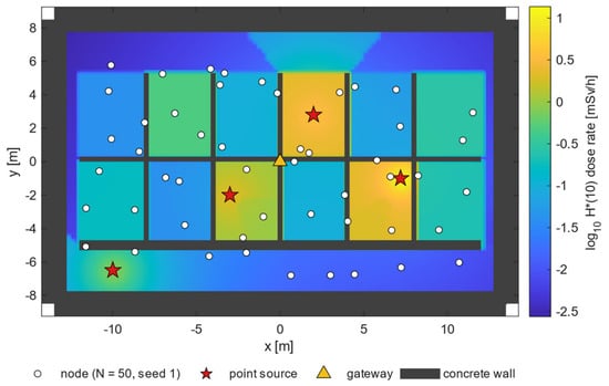
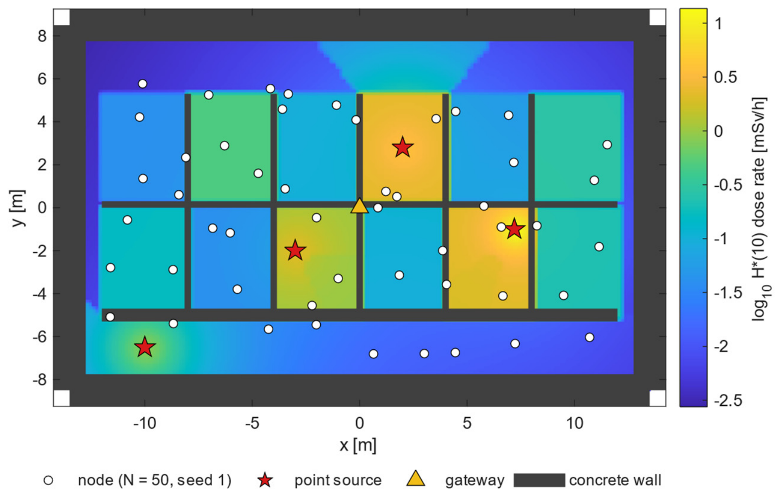
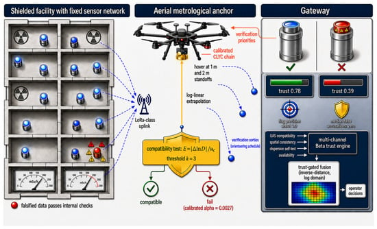
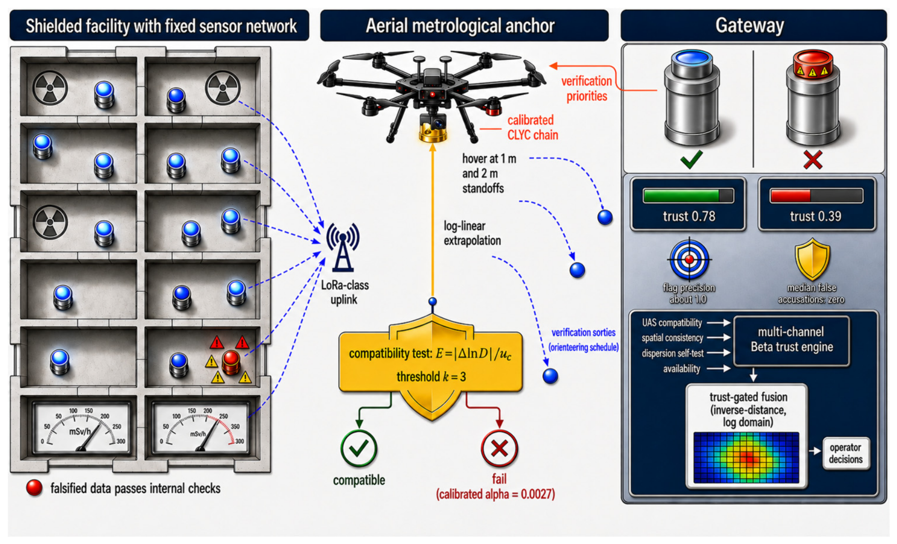
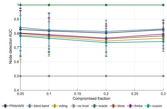
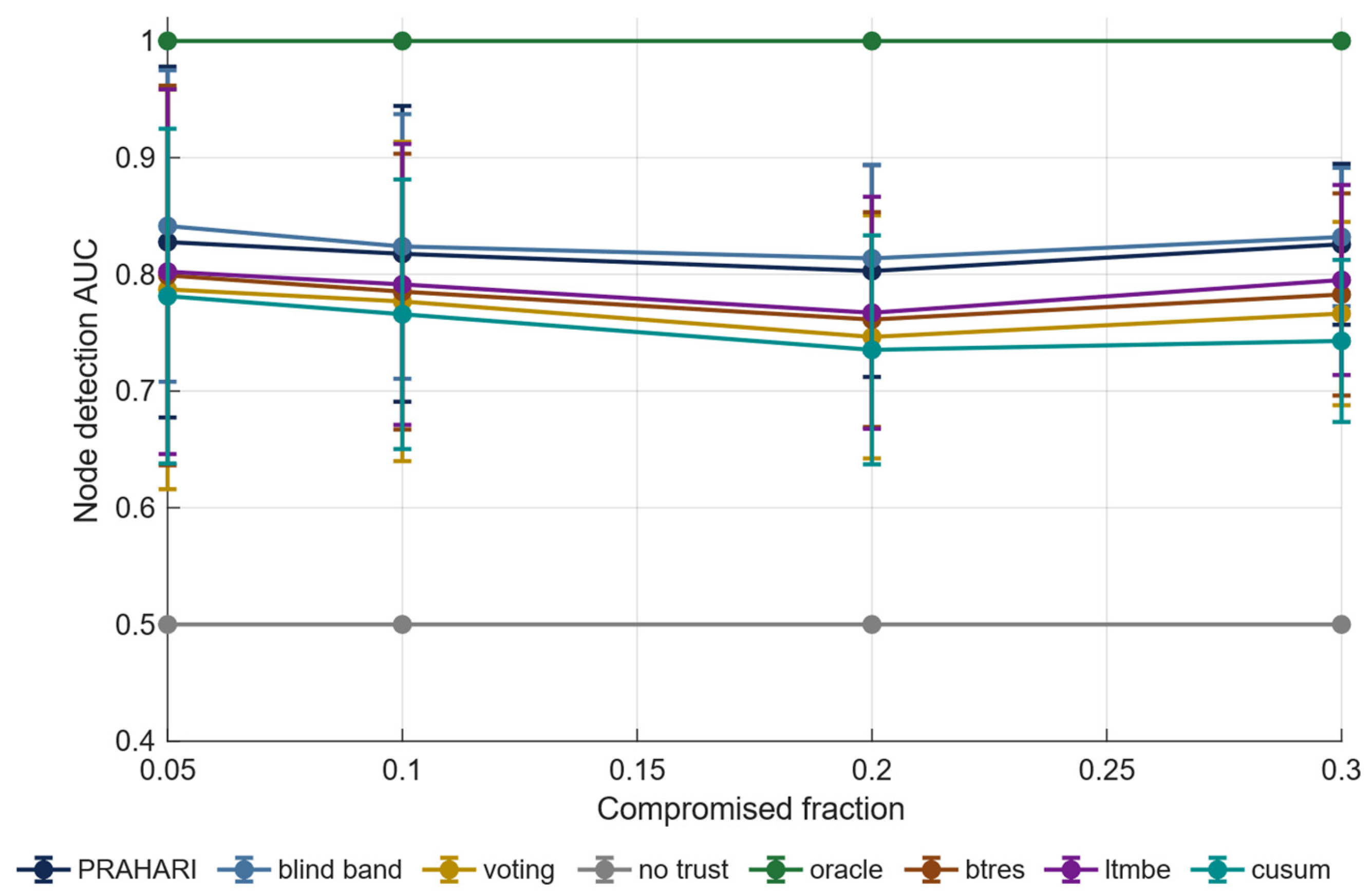
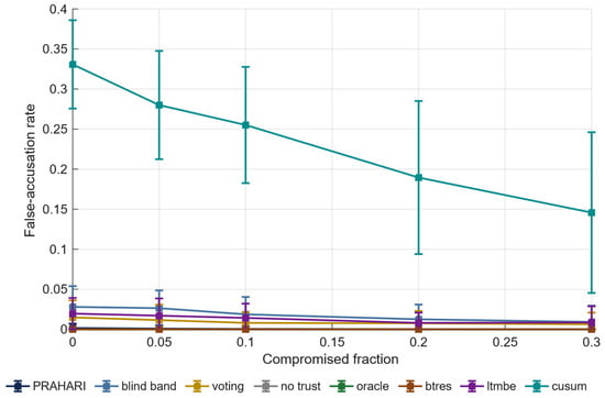
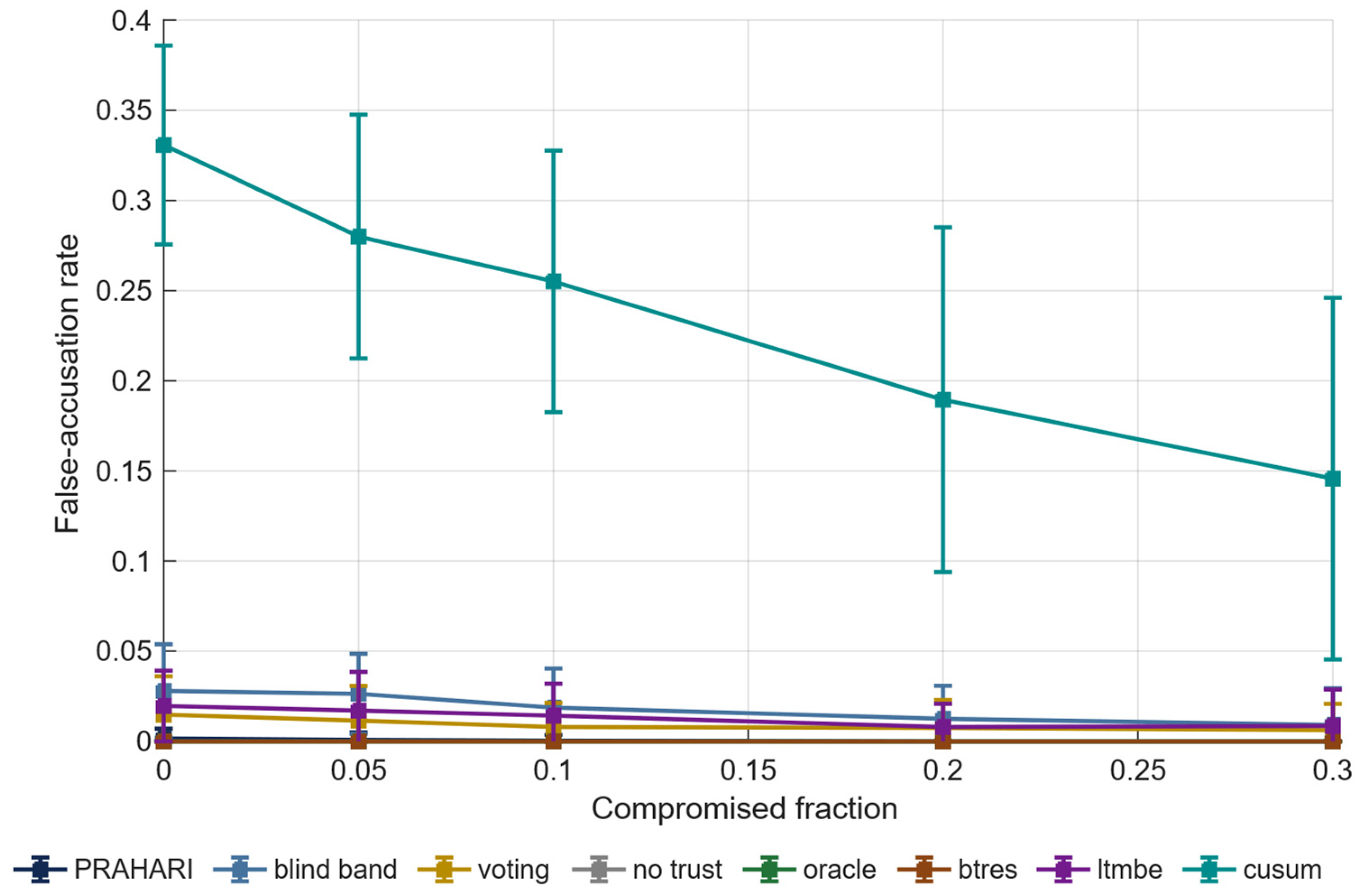
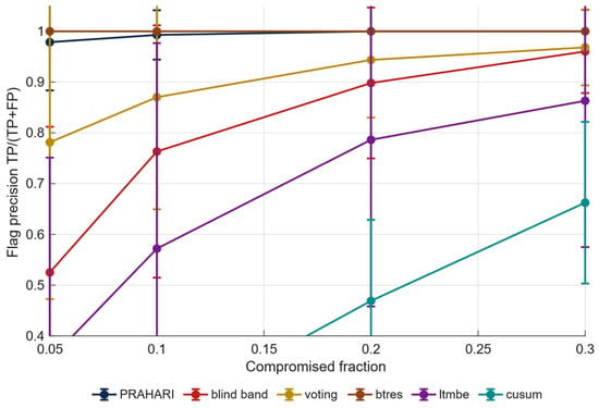
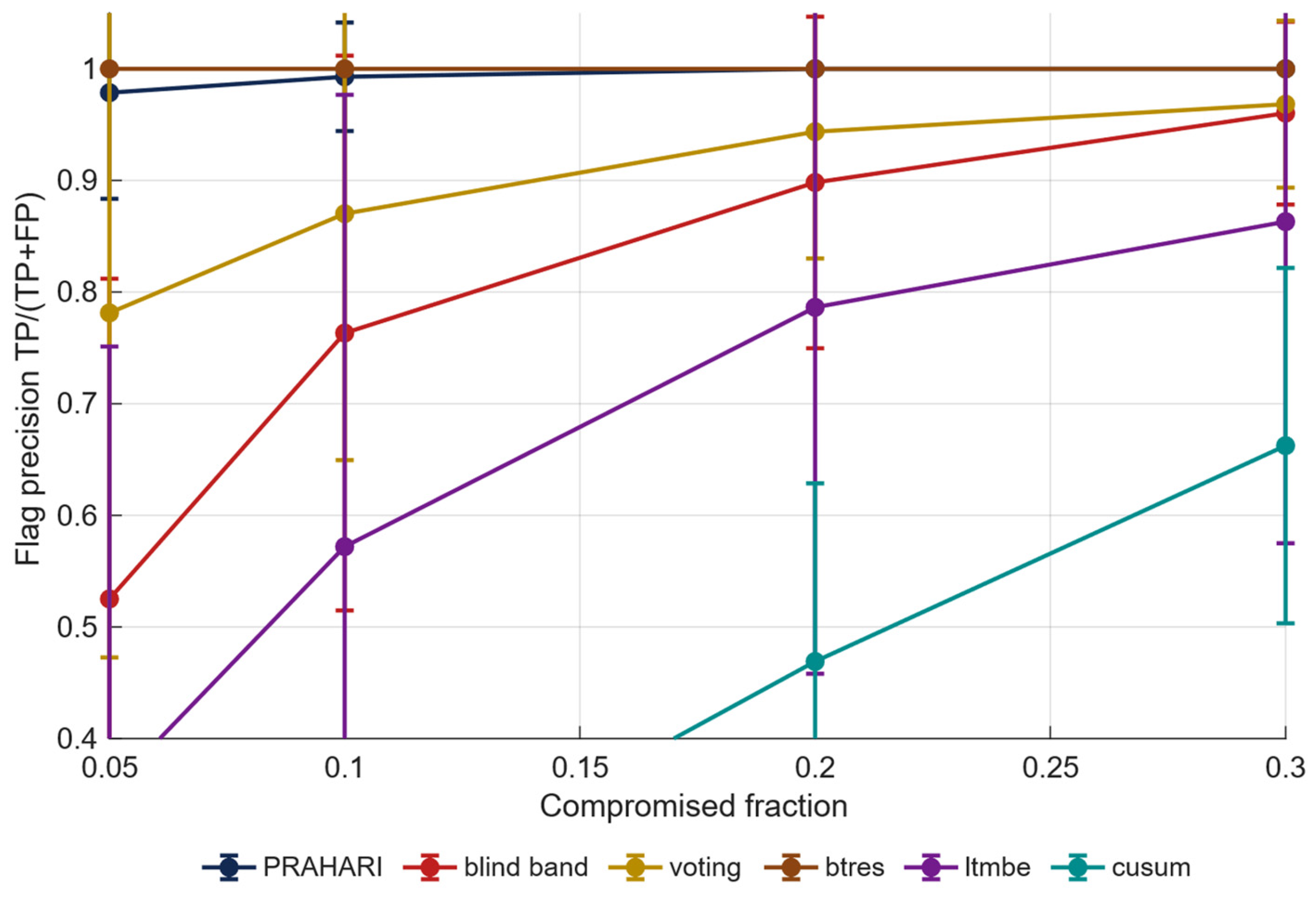
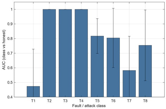
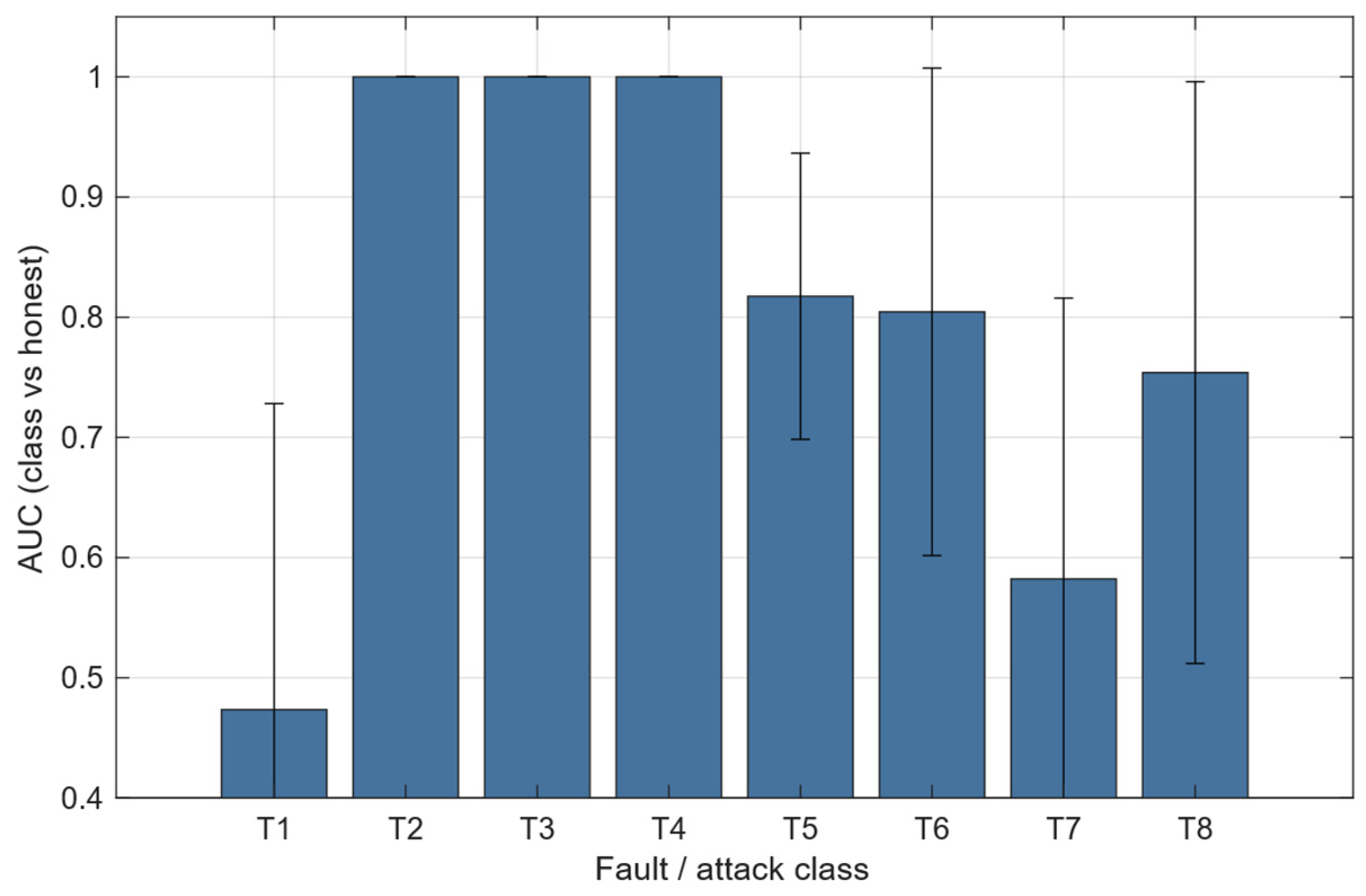
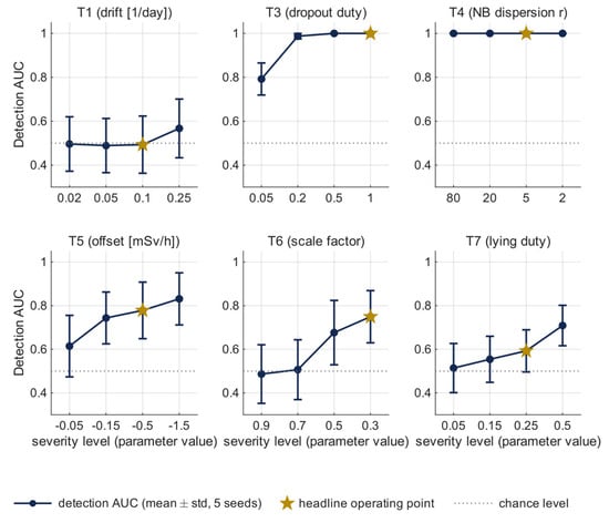
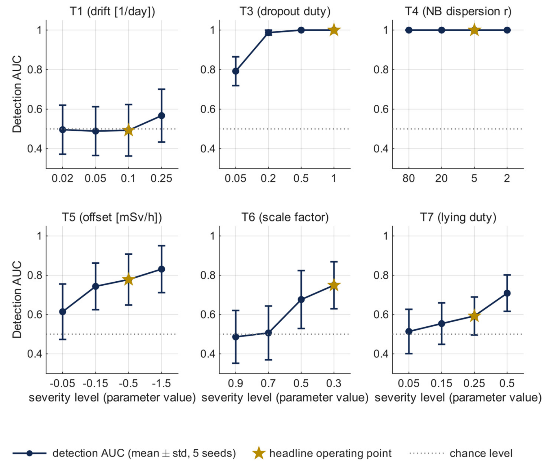
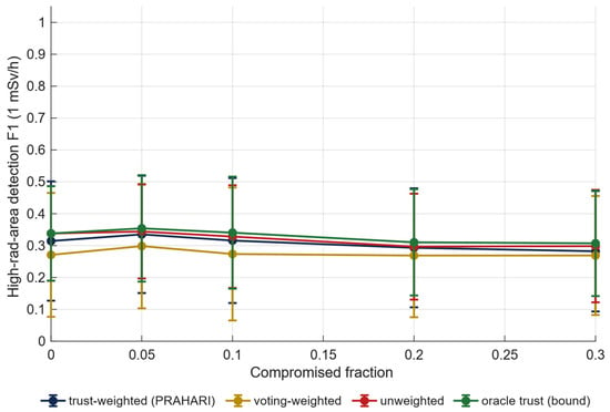
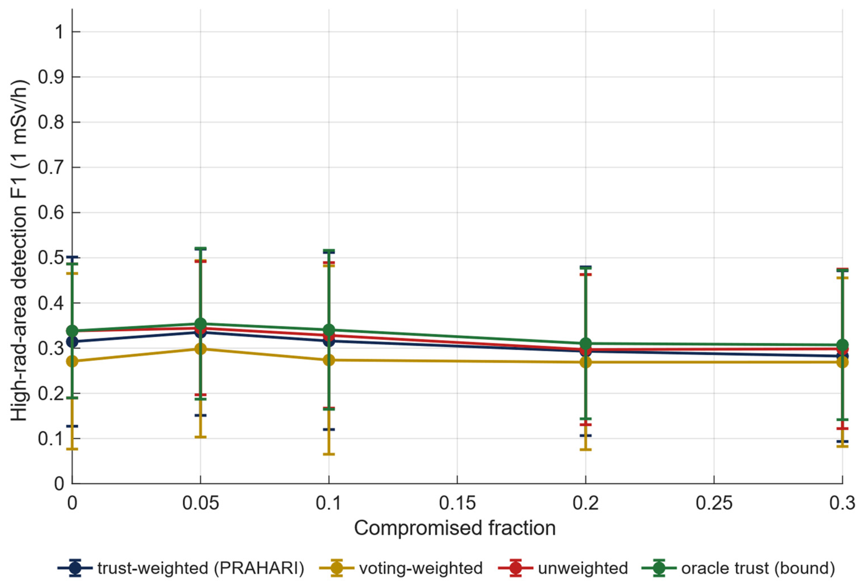
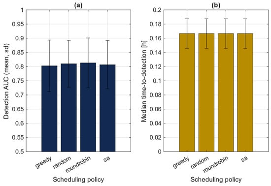
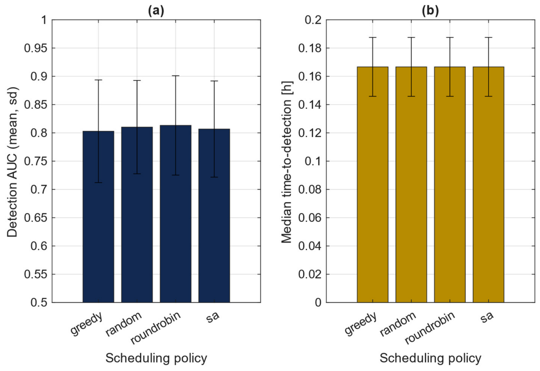
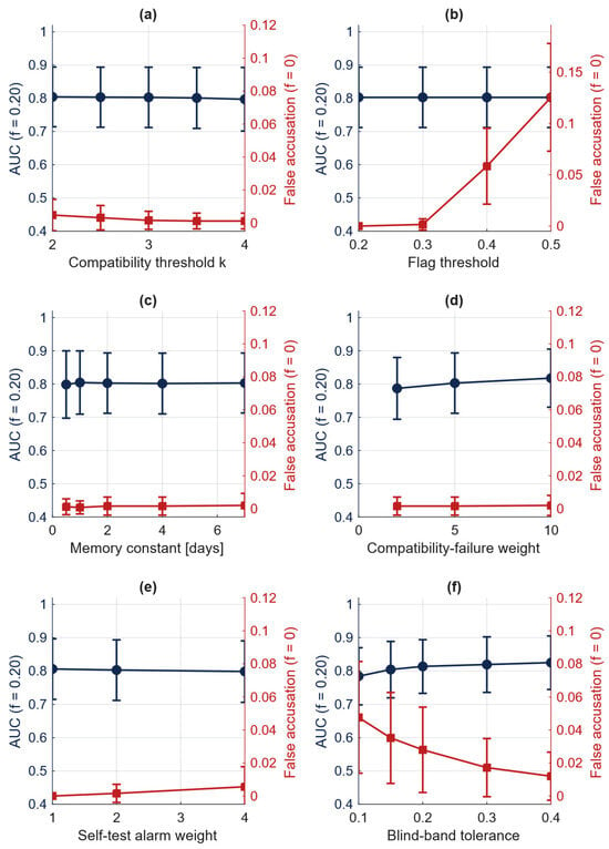
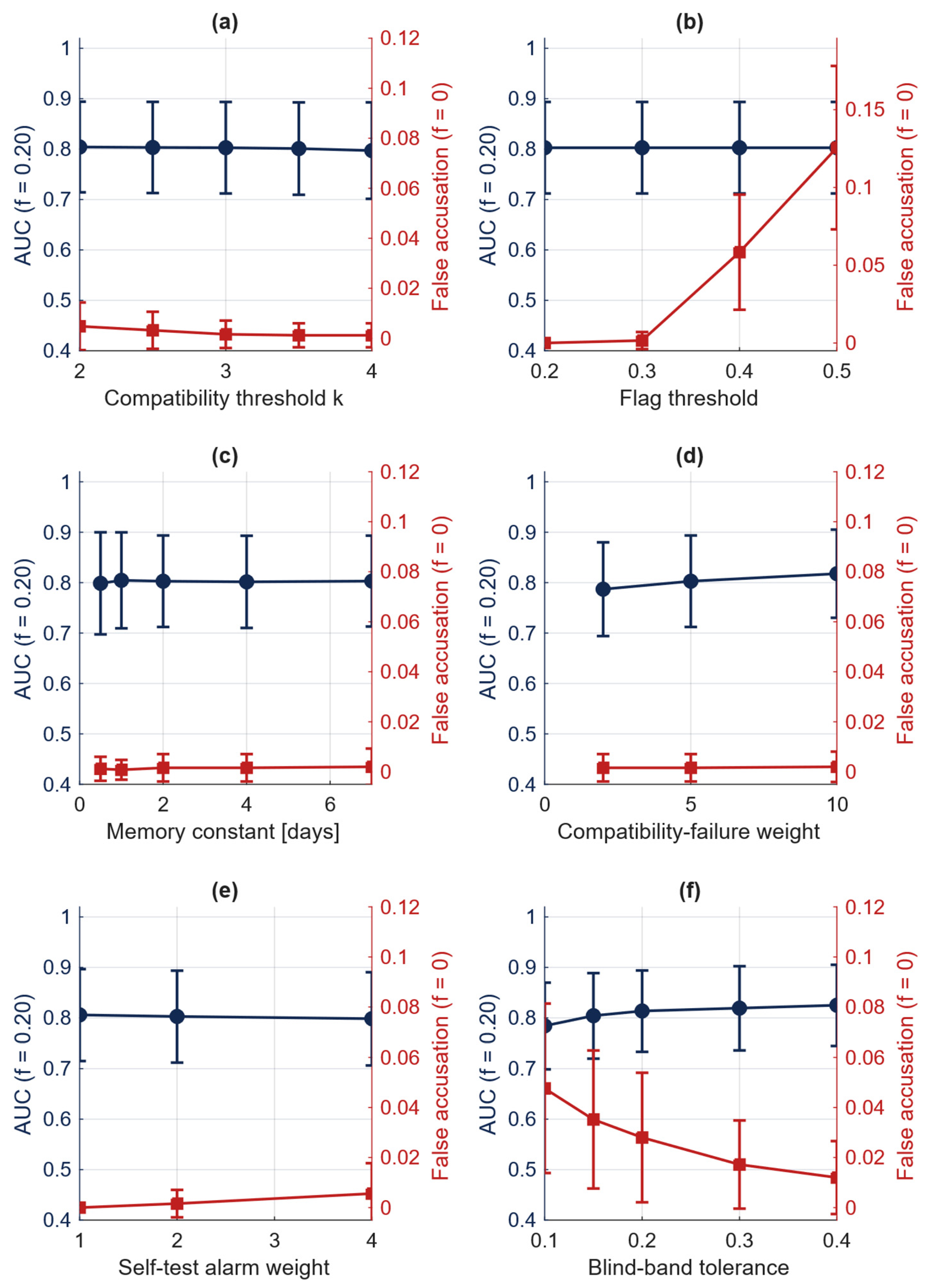
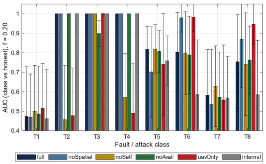
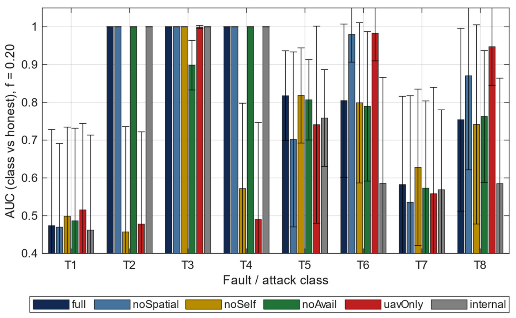
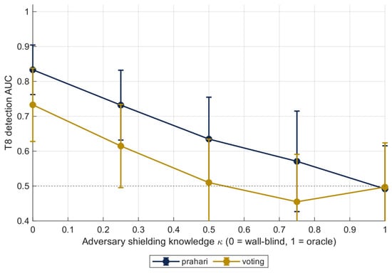
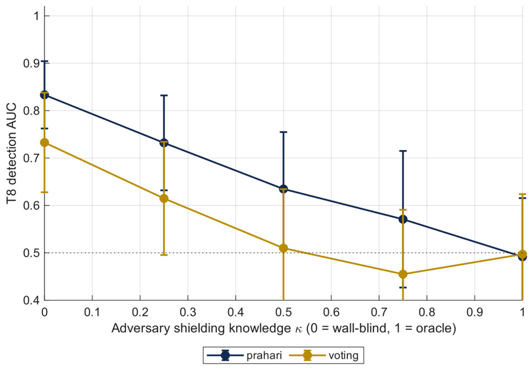
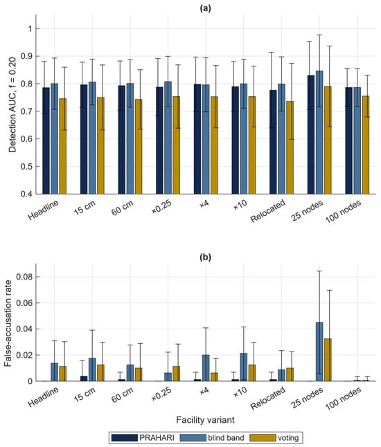
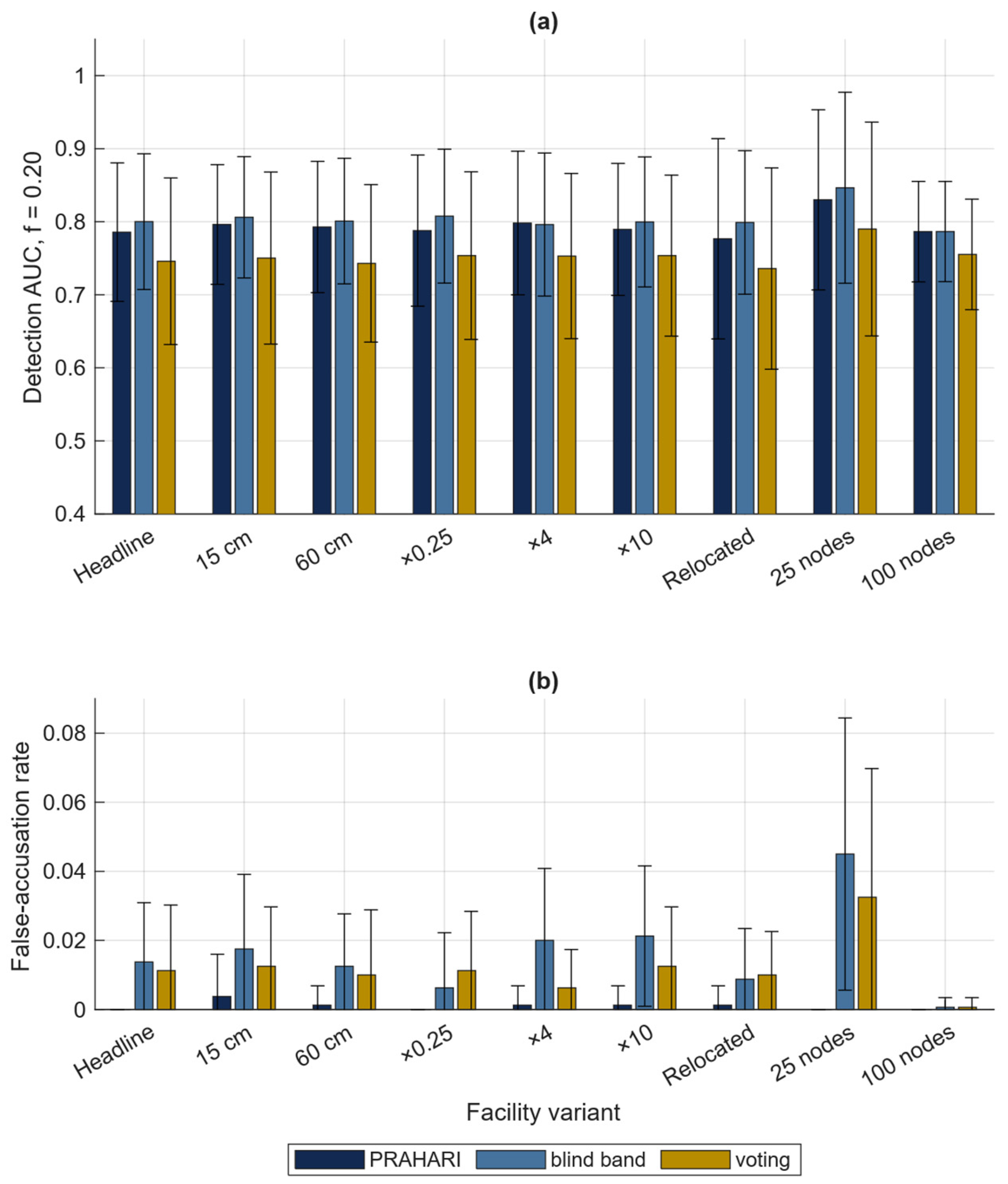
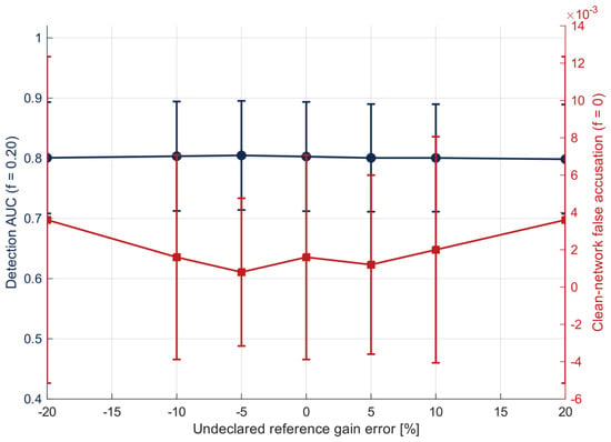
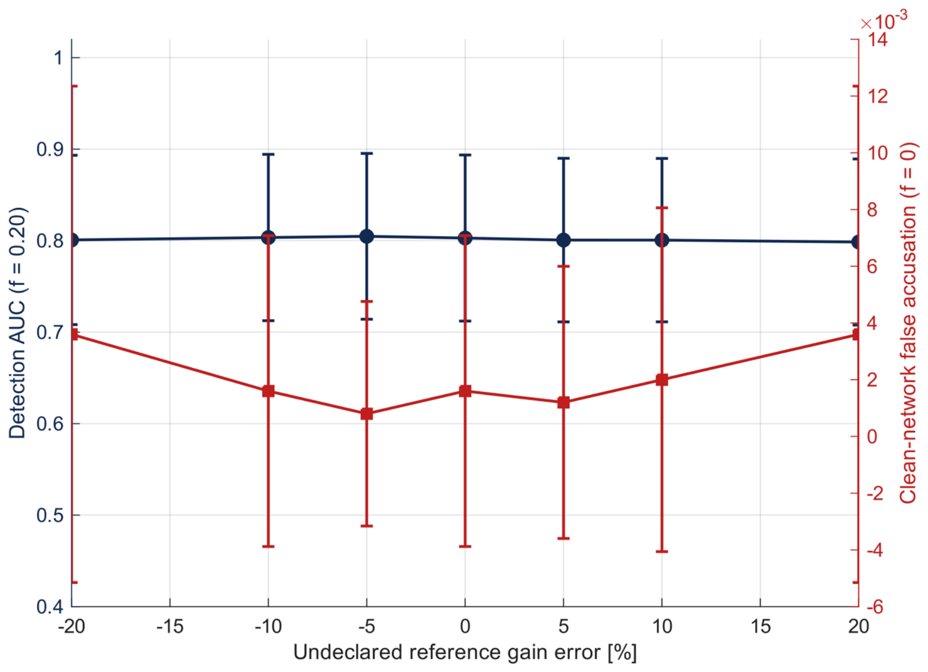
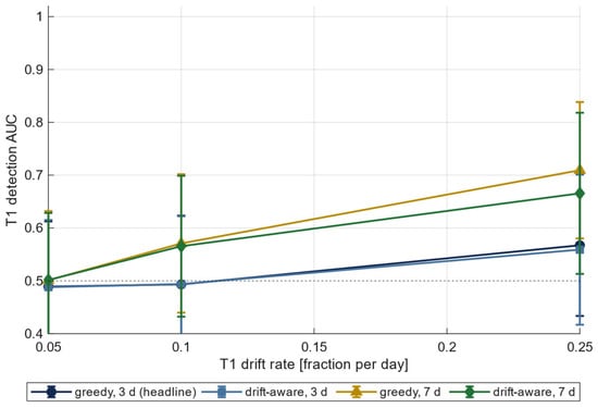
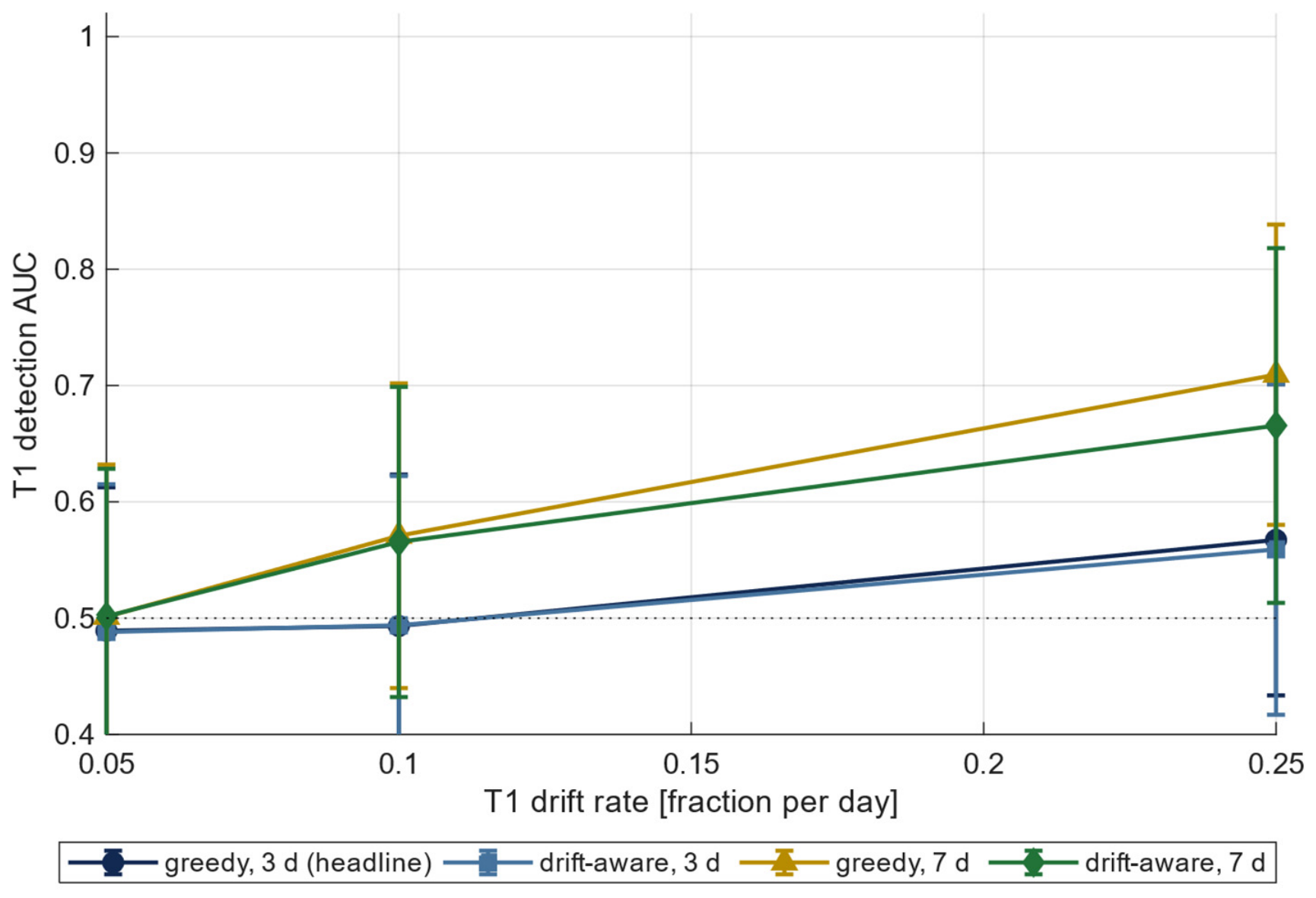

Disclaimer/Publisher’s Note: The statements, opinions and data contained in all publications are solely those of the individual author(s) and contributor(s) and not of MDPI and/or the editor(s). MDPI and/or the editor(s) disclaim responsibility for any injury to people or property resulting from any ideas, methods, instructions or products referred to in the content. |
© 2026 by the authors. Licensee MDPI, Basel, Switzerland. This article is an open access article distributed under the terms and conditions of the Creative Commons Attribution (CC BY) license.