


Abstract
Mechanized timber harvesting on steep slopes causes soil disturbance; however, comprehensive post-harvest assessment remains challenging because terrain complexity and safety constraints render traditional field-based methods labor-intensive, spatially limited, and difficult to implement systematically. In this study, we developed and evaluated a convolutional neural network-based semantic segmentation model for detecting soil disturbances using high-resolution unmanned aerial vehicle (UAV) imagery in a steep-slope harvested area (2.50 ha, mean slope of 53.4%) in Republic of Korea. A U-Net semantic segmentation model was trained on manually annotated orthomosaic tiles incorporating RGB and digital elevation model (DEM) inputs. Ensemble predictions at an optimized threshold of 0.65 achieved Intersection over Union (IoU) of 0.55 and F1-score of 0.71. Although moderate, these values reflect the inherently challenging conditions of steep-slope forest terrain compared to similar studies conducted under gentler terrain. DEM-derived depth estimation enabled severity classification of the detected disturbances, with light disturbances predominating. Field validation using 38 pinboard measurements demonstrated reliable spatial detection (ρ = 0.567, RMSE = 6.45 cm). This approach provides an effective alternative to traditional monitoring practices in mountainous forests, where systematic trail planning is impractical, and may support evidence-based assessment of harvesting impacts for sustainable forest management.
1. Introduction
The global forest industry has undergone a profound transformation in timber harvesting practices over the past several decades, with mechanized operations increasingly replacing traditional manual methods. The widespread use of forestry machinery reflects converging pressures: the need for greater operational efficiency, improved worker safety, and responses to workforce aging and recruitment difficulties [1,2].
Although mechanized harvesting has become indispensable in modern forest management, its environmental footprint on forest soils has emerged as a considerable concern. From a soil mechanical perspective, the risk of soil disturbance can be better understood by comparing machine-induced stresses with the load-bearing capacity of the soil. The load-bearing capacity of loamy forest soils is typically reported to range from approximately 80–120 kPa under optimal moisture conditions, decreasing to 30–60 kPa under wetter conditions [3]. Ground pressure exerted by forestry machinery typically ranges from approximately 30 to 75 kPa, while stresses transmitted into the soil can exceed 200 kPa and reach up to 400–500 kPa depending on machine type and operating conditions [4,5,6]. Repeated traffic by such equipment, including harvesters, forwarders, and skidders, inevitably causes soil compaction and rutting [7,8]. The effects of these physical disturbances extend far beyond visible surface deformation. Soil compaction typically increases the bulk density and reduces the total porosity in trafficked areas [9], fundamentally altering the physical architecture of the soil. These changes restrict root penetration and growth [10], impair water infiltration and drainage patterns [11], and reduce soil aeration [12], and persist for decades in the absence of active restoration [13,14]. Additional effects include modified microbial communities [15], altered nutrient cycling processes [16], and increased emissions of greenhouse gases, such as nitrous oxide and methane from anaerobic microsites [17,18]. Accurate post-harvest monitoring of soil disturbance is therefore essential for both operational forestry and broader ecosystem functions, including carbon sequestration, hydrological regulation, and forest regeneration, within the context of sustainable forest management.
The awareness of these environmental consequences has led to the development and improvement of various soil protection strategies. Seasonal restrictions represent a commonly used approach, whereby operations are planned to prevent soil disturbance during periods of saturation and increased vulnerability to compaction, typically during spring thaw or prolonged wet weather [19]. The application of harvesting residues in designated machine operating trails effectively distributes loads and maintains soil structure [20]. The systematic planning approach is potentially the most influential method, in which harvesting operations follow predetermined trail networks designed to confine soil disturbances to specific machine trails [21].
However, the applicability of conventional soil protection strategies to steep-slope forestry operations is limited by terrain-related constraints [22]. Seasonal restrictions depend on predictable weather windows and accessible monitoring, both of which are difficult to enforce on steep and remote sites. Residue application requires sufficient slash material distributed along designated trails [23], yet on steep terrain, the unpredictable nature of machine routes makes systematic residue placement impractical. Trail planning assumes that operators can adhere to predefined routes. In mountainous environments, however, machine stability and operator safety take precedence, requiring flexible positioning and route adjustments in response to local terrain conditions. Consequently, maintaining strictly predefined trail networks can be challenging, and soil disturbances may not always be confined to designated corridors. Under these conditions, post-harvest assessment may represent a practical complement to preventive measures.
Soil disturbance severity has traditionally been evaluated using a range of field-based techniques such as penetration resistance measurements, laboratory analyses of soil physical and chemical properties, and morphological profiling with tools such as pinboards, chains, and rulers [24,25,26]. Although these approaches provide comprehensive and site-specific information, their application is time-consuming and typically confined to discrete sampling locations. To address these limitations, remote sensing approaches, particularly photogrammetric reconstruction and mobile laser scanning-derived three-dimensional surface models, are increasingly used to quantify soil surface deformation across broader spatial extents with improved consistency and repeatability [27,28].
Unmanned aerial vehicle (UAV) technology has become increasingly valuable for forest monitoring, offering spatial coverage and resolution that complement ground-based methods. Whereas field-based surveys are typically limited to discrete sampling points and require considerable time to cover harvested areas of several hectares [29], modern commercial UAVs equipped with high-resolution RGB cameras can capture imagery at ground sampling distances of 1–3 cm across several hectares within 1–2 h of flight time [30]. The integration of structure-from-motion (SfM) photogrammetric processing has further improved the utility of UAV platforms, facilitating the generation of digital elevation models (DEMs) and orthomosaics with vertical and horizontal accuracies typically within 2–5 cm [31]. Beyond UAV-based photogrammetry, LiDAR-based approaches offer higher geometric accuracy for soil disturbance quantification; however, their operational costs and equipment requirements limit widespread adoption in routine post-harvest monitoring [32].
The analytical potential of high-resolution UAV imagery has been increased by concurrent advances in image analysis methods, particularly in the application of deep learning algorithms. Traditional photogrammetric methods and shallow learning classifiers, such as random forests and support vector machines, have been widely applied to forest disturbance mapping. However, their performance often depends on manually engineered features and may be limited in capturing complex spatial patterns in heterogeneous environments [33,34]. Convolutional neural networks (CNNs) are highly effective in extracting complex spatial patterns from remote sensing data, consistently outperforming traditional pixel- or object-based classification approaches [33]. Among deep learning architectures, semantic segmentation models, such as U-Net, SegNet, and DeepLab, have been extensively applied in forestry applications, demonstrating strong pixel-level classification performance [35,36]. These properties are especially relevant for mapping machine-induced rutting and surface deformation, which exhibit irregular geometries and context-dependent visual variability that make data-driven segmentation approaches particularly advantageous [37].
Despite the growing availability of high-resolution UAV imagery and advances in deep learning, automated mapping and severity classification of machinery-induced disturbances in steep-slope harvesting environments remains an unresolved challenge. Existing methods have not been widely explored under the complex terrain conditions characteristic of mountainous forestry operations, where the reliable identification and classification of harvesting-induced disturbances remains particularly challenging. The present study addresses this gap through three methodological contributions: the application of CNN-based semantic segmentation for automated disturbance mapping in extremely steep terrain (mean slope 53.4%); the integration of DEM-derived depth estimation for quantitative severity classification; and the validation of the approach against field-based pinboard measurements under operational harvesting conditions.
This study aimed to: (1) develop a CNN-based semantic segmentation model for identifying and mapping soil disturbances caused by forestry machinery in steep-slope harvesting areas using high-resolution UAV RGB imagery; (2) evaluate the model performance through comparison with independent field-based reference measurements; and (3) quantify the spatial extent and distribution characteristics of identified soil disturbances within the study site. We hypothesized that integrating UAV-derived high-resolution imagery with CNN-based semantic segmentation can provide accurate and scalable detection of soil disturbance in steep-slope harvesting environments, where terrain complexity renders traditional monitoring methods impractical. Specifically, we expect that (1) the U-Net model will achieve practically meaningful segmentation performance for detecting machinery-induced soil disturbances from RGB imagery; and (2) DEM-based depth estimation will enable ecologically relevant severity classification of detected disturbances, supporting evidence-based assessment of harvesting impacts on forest soils.
2. Materials and Methods
2.1. Study Area and Harvesting Operation
This study was conducted in a steep-slope harvested area within the experimental forest of Kangwon National University (37°50′18.6″ N, 127°50′0.38″ E, 615 m a.s.l.). The study site covered approximately 2.50 ha with a mean slope of 53.4%, representing a relatively steep terrain. The terrain exhibited considerable variability, with slopes ranging from 6.4% to 69.3%, reflecting heterogeneous topographic conditions that likely contributed to spatially variable soil disturbance patterns across the site.
According to the Köppen climate classification, the site had a humid continental climate with hot summers [38]. Over the past 30 years (1996–2025), the mean annual temperature was 11.19 °C, while the mean annual precipitation was approximately 1339.27 mm. The soil was classified as a Mui series according to the U.S. soil taxonomy, with a loam texture consisting of 52.4% sand, 12.5% clay, and 35.2% silt [39].
The harvested area comprised a deciduous broadleaf stand dominated by oak species with 1041 trees. The species composition was as follows: other broadleaf species accounted for 721 trees (69.3%), Larix kaempferi (Lamb.) Carrière comprised 193 trees (18.5%), Quercus mongolica Fisch. ex Ledeb. represented 66 trees (6.3%), Pinus koraiensis Siebold & Zucc. constituted 47 trees (4.5%), and Quercus variabilis Blume consisted of 14 trees (1.3%). The mean diameter at breast height (DBH) of the entire stand was 21.3 cm, with a mean individual tree volume of 0.45 m3. Pinus koraiensis was excluded from harvesting to prevent the spread of pine wilt disease.
The harvesting operations were completed on 9 June 2023. The felling and bucking operations were performed using a chainsaw (STIHL MS361; STIHL, Waiblingen, Germany), followed by extraction using an excavator (Hyundai HX 65 AMT; Hyundai, Seoul, Republic of Korea) equipped with a wood grapple. The excavator had an operating weight of 6.39 t (excluding wood grapple) and was equipped with a crawler wheel. Each wheel measured 1990 mm in length and 380 mm in width, resulting in a ground contact area of approximately 0.76 m2 per track.
Owing to the steep topographic conditions of the site, systematic preplanning of machine travel routes was not feasible. Consequently, the operator made real-time decisions based on machine stability and safety considerations and selected relatively accessible routes during operations. The excavator grasped felled logs with a wood grapple and threw them downslope toward the forest road located at the lower portion of the site.
The entire machine operation was recorded to enable post hoc analysis of machine traffic. However, due to limitations in visibility and recording conditions, it was not possible to identify all machine passes across the site. Despite these limitations, repeated use of certain routes was clearly observed, with up to five machine passes identified along the same track. This pattern likely reflects the operator’s preference for relatively stable and accessible paths to ensure safe machine operation under steep terrain conditions.
2.2. UAV Data Acquisition and Processing
To capture the spatial distribution of soil disturbance across the study site, aerial photography was conducted on 18 June 2023, using a UAV (Matrice 300, DJI Enterprise, Shenzhen, China) equipped with a 20-megapixel RGB camera (Zenmuse H20T, DJI Enterprise). The UAV flew at an altitude of approximately 70 m above ground level with a mean flight speed of 3 m/s. Both forward and side overlaps were set to 90% to ensure adequate image coverage. The designed flight path covered a total length of approximately 2255 m over a mapping area of approximately 3 ha (30,282 m2). A total of 297 aerial images were acquired in the autonomous flight mode.
The acquired aerial images were processed using Agisoft Metashape Professional software (version 1.5.1, Agisoft LLC, St. Petersburg, Russia). SfM photogrammetry was employed to perform image alignment and generate a 3D dense point cloud. Based on this process, an orthomosaic DEM with a spatial resolution of approximately 2.33 cm/pixel was generated. The generated orthophotos served as input data for the subsequent CNN-based disturbance mapping analysis.
2.3. Data Annotation and Preparation
The generated orthophotos were divided into non-overlapping tiles of 256 × 256 pixels for CNN model training, resulting in 1962 image tiles. Specifically, 832 tiles containing clearly visible soil surfaces were selected, excluding the forest interior areas covered by canopy. From this subset, 450 tiles were selected for manual pixel-wise annotations. Soil disturbance areas were defined as regions in which morphological changes to the ground surface were clearly identifiable through visual inspection, including crawler tracks (wheel ruts), soil displacement, and exposed mineral soil resulting from harvesting and extraction operations.
Tile generation and preliminary tile selection were conducted in QGIS (version 3.24.2, Open Source Geospatial Foundation, Beaverton, OR, USA). Manual pixel-wise annotation was then performed using a custom Python-based labeling interface built with OpenCV (version 4.13.0) and rasterio (version 1.4.4). The annotation workflow was designed to display the target tile together with adjacent DEM tiles to provide local topographic context during delineation. All annotations were performed by a single operator following consistent visual criteria, and the labeled masks were reviewed during the annotation process to minimize obvious labeling inconsistencies.
2.3.1. Annotation Procedure
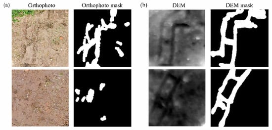
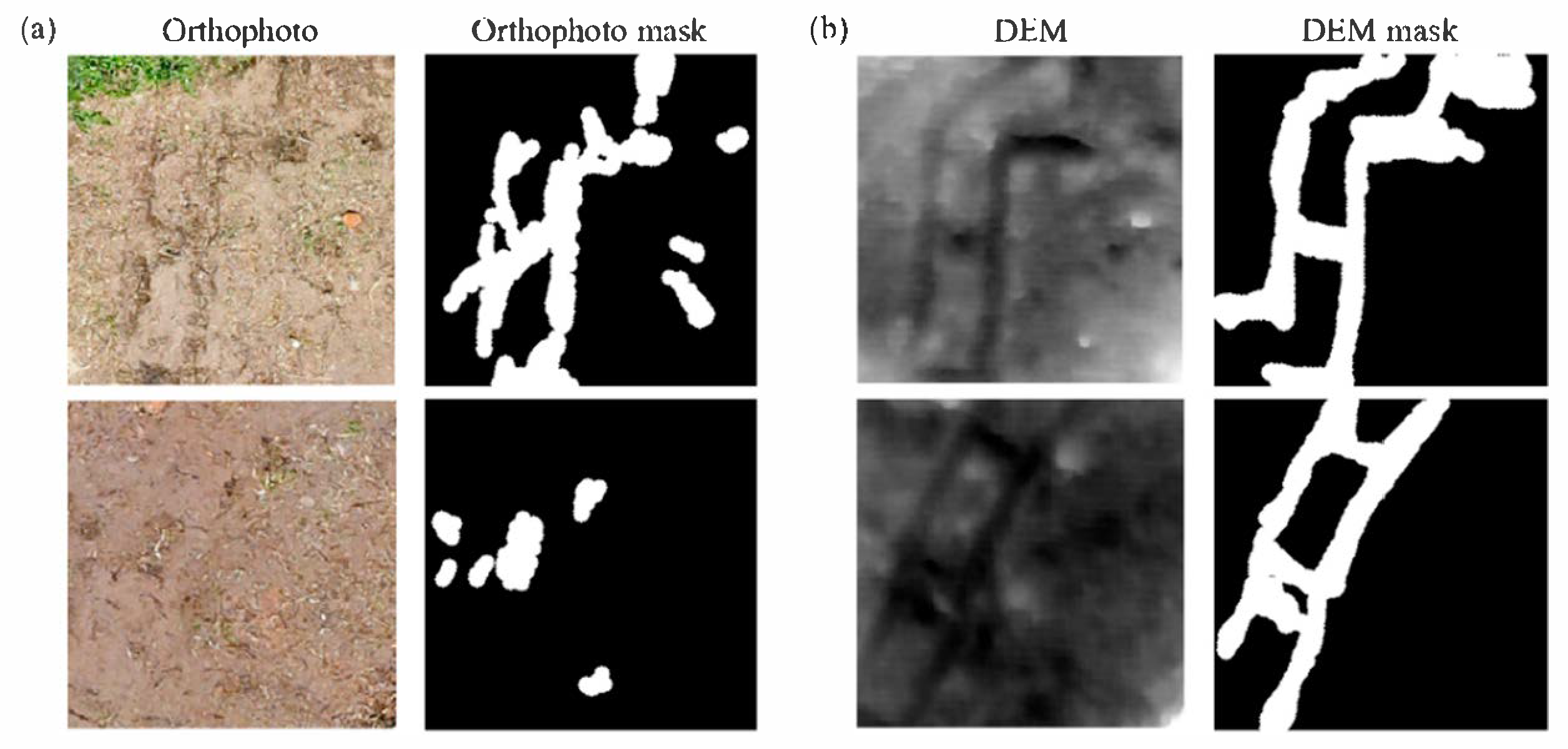
The annotation of the soil disturbance areas was primarily performed based on RGB orthomosaic imagery (Figure 1a), as widely adopted in UAV-based assessments of forest soil disturbance [37,40]. Regions exhibiting visually identifiable soil disturbance characteristics (color changes, surface texture alterations, and crawler tracks) in the RGB orthomosaic were manually delineated as disturbance areas.
Figure 1.
Examples of (a) orthophoto and (b) digital elevation model (DEM) inputs with corresponding soil disturbance masks.
The DEM served as auxiliary information during the annotation process (Figure 1b). Before annotation, the DEM was detrended by subtracting a least-squares fitted global plane, and the resulting residual surface was robustly normalized to a 0–1 range using the 1st and 99th percentiles. The normalized DEM was then resampled to match the RGB tile grid and used to assist in the delineation of disturbance boundaries in visually ambiguous areas. However, the primary identification of disturbance areas relied on RGB information, with DEM used only as supplementary evidence for boundary refinement and ambiguous cases.
2.3.2. Data Partitioning
To enable consistent performance comparisons across multiple training runs while reducing spatial autocorrelation between adjacent samples, the tiles were grouped into 2 × 2 tile-based spatial blocks based on their row and column indices. This block size was selected as a pragmatic balance between reducing spatial autocorrelation between adjacent samples and maintaining sufficient sample size for cross-validation, given the limited number of annotated tiles (n = 450). Blocks were randomly assigned, and 15% of the blocks (representing approximately 68 tiles; 15.1%) were reserved as a fixed test set. This test set remained completely separate during all training iterations and was used exclusively for final model evaluation.
The remaining 85% of the blocks (approximately 382 tiles, 84.9%) were further partitioned using five-fold cross-validation. In each fold, the training-validation blocks were divided into five subsets. One subset was the validation set for that fold, whereas the remaining four subsets formed the training set. This process was repeated five times, with each subset serving as a validation set exactly once. The final split for each fold was as follows: training, 314 tiles (69.8% of the total); validation, 68 tiles (15.1% of the total); and test, 68 tiles (15.1% of the total).
2.4. CNN-Based Soil Disturbance Detection
2.4.1. Model Architecture
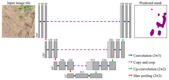
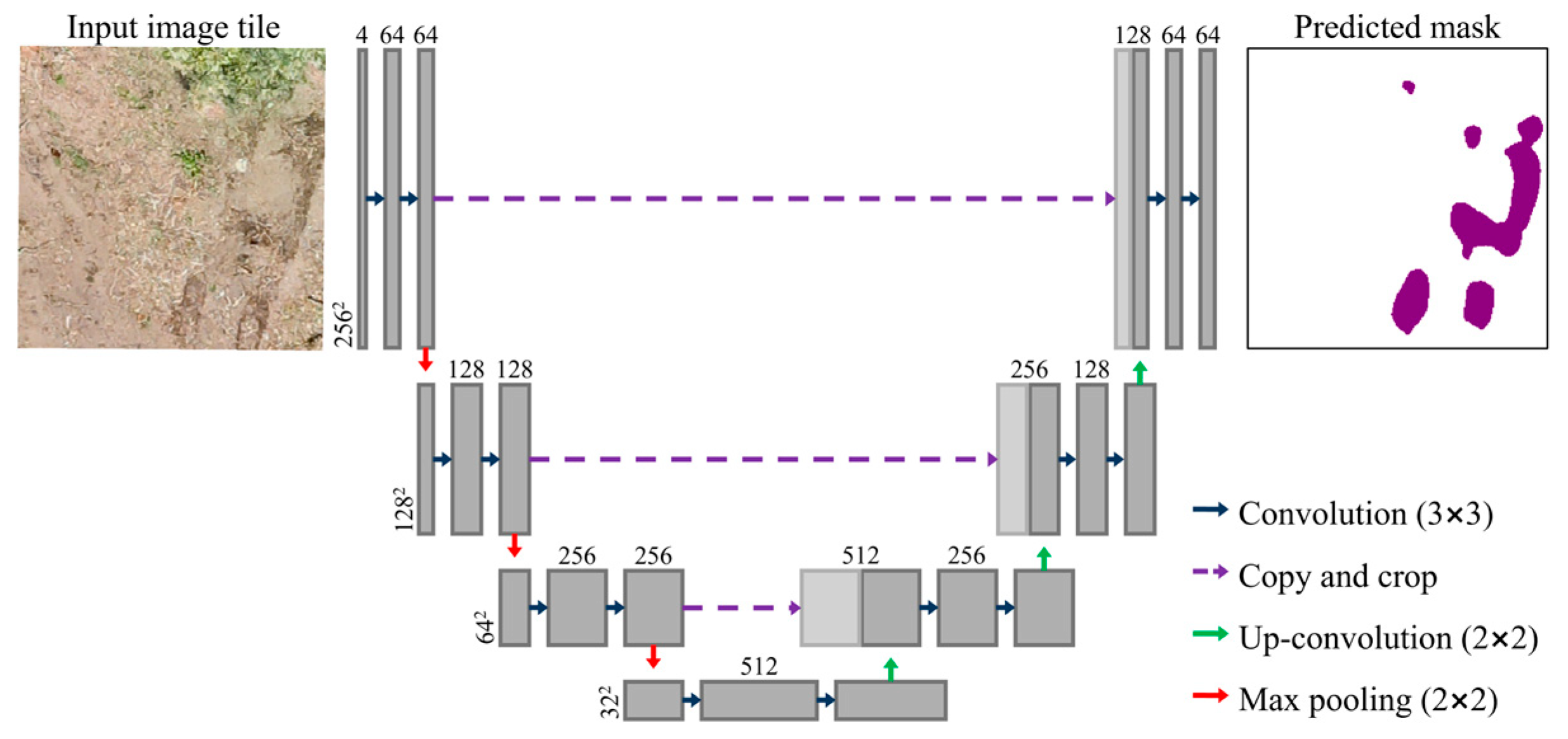
A U-Net CNN architecture [41] was employed for the pixel-wise detection of soil disturbance areas (Figure 2). U-Net was selected for its well-established performance in high-resolution remote sensing segmentation with limited training data, its encoder–decoder structure enabling precise boundary delineation via skip connections, and its computational efficiency. More complex architectures, such as Attention U-Net, U-Net++, and transformer-based models, impose substantially higher data and computational requirements, which may not be justified given the single-site dataset used in this study. U-Net is a fully convolutional network with an encoder–decoder structure, where the encoder progressively extracts hierarchical features from the input image, and the decoder reconstructs the pixel-wise classification at the original resolution. The model was designed to leverage the complementary information from both RGB and DEM data. The input consisted of 256 × 256 × 4 tiles comprising three RGB channels (red, green, and blue) and one normalized DEM channel.
Figure 2.
U-Net architecture used for soil disturbance semantic segmentation.
The U-Net architecture implemented in this study consisted of three downsampling stages in the encoder and three upsampling stages in the decoder. The three-stage configuration was selected to preserve fine-grained spatial details critical for detecting small and irregularly shaped soil disturbance patches. Each encoder stage comprised a DoubleConv block consisting of two sequential 3 × 3 convolution layers with batch normalization and ReLU activation, followed by 2 × 2 max pooling for spatial downsampling. Through successive pooling operations, the spatial resolution of the input was progressively reduced from 256 × 256 to 128 × 128, 64 × 64, and 32 × 32 pixels, and the number of feature channels increased accordingly. A base parameter of 64 was used, resulting in 64, 128, 256, and 512 feature channels at each encoder level.
The decoder followed a symmetrical design similar to the encoder, with each stage consisting of a 2 × 2 transpose convolution for upsampling, concatenation with the corresponding encoder feature maps through skip connections, and a DoubleConv block. Skip connections transferred high-resolution spatial information from the encoder to the decoder, enabling precise boundary delineation of disturbance areas. A 1 × 1 convolution was applied in the final output layer, followed by sigmoid activation, to generate a probability map (values between 0 and 1), indicating the likelihood of soil disturbance for each pixel.
All the network weights were initialized randomly without using pretrained weights. The model was implemented using PyTorch (version 2.5.1) and trained using an NVIDIA GeForce RTX 1660 GPU.
2.4.2. Training Procedure
The model training employed a combined loss function that incorporated Binary Cross-Entropy (BCE) loss and Dice loss to address the characteristics of the binary segmentation task. The BCE loss minimizes pixel-level classification errors, whereas the Dice loss maximizes the overlap between the predicted and ground-truth regions, thereby mitigating class imbalance issues. The two loss functions were weighted equally (0.5 each) to balance the pixel-wise accuracy and spatial continuity of soil disturbance areas.
To address the pixel-level class imbalance further, per-pixel weighting was applied within the loss functions, following the principle of weighting each pixel’s contribution to the loss function based on its annotation reliability [42]. Pixels in regions with high annotation confidence (RGB-identified disturbances) were assigned a full weight (w = 1.0), whereas pixels in regions with lower confidence (DEM-identified but RGB-ambiguous) received a reduced weight (w = 0.3). The specific weight value was determined empirically to balance the contribution of weak labels without suppressing their auxiliary information. This differential weighting strategy enabled the model to prioritize learning from high-confidence annotations, while incorporating auxiliary information from DEM-based weak labels.
The Adam optimizer was employed with an initial learning rate of 0.001. The batch size was set to eight based on GPU memory constraints. The maximum number of training epochs was set to 200.
To prevent overfitting, an early stopping mechanism was applied based on the validation of the intersection over union (IoU) metric. Training was terminated if validation IoU did not improve by at least 10−4 for 30 consecutive epochs. The best model for each fold was defined as the epoch that achieved the highest validation IoU, and its weights were saved for subsequent evaluations.
Owing to the relatively low proportion of tiles containing soil disturbance pixels, tile-level weighted random sampling was implemented during the training. Tiles containing one or more soil disturbance pixels were assigned a sampling weight of 8.0, whereas tiles without disturbance pixels were assigned a weight of 1.0, ensuring a higher sampling probability for disturbance-containing tiles in each epoch. This approach enabled the model to effectively learn sparse soil disturbance patterns without being overwhelmed by the majority class (undisturbed background).
To enhance the model generalization, simple data augmentation techniques were applied exclusively to the training data. The horizontal and vertical flips were randomly applied with a probability of 0.5 each. These geometric transformations were appropriate for this task because the soil disturbance patterns exhibited no inherent directional bias. No augmentation was applied to the validation or test data to ensure unbiased performance evaluation.
2.4.3. Threshold Selection and Performance Metrics
The trained model outputted a continuous probability map (0–1) for each pixel. For fold-wise evaluation, an optimal threshold was independently determined for each fold by maximizing the F1-score on the validation dataset. Thresholds ranging from 0.10 to 0.90 were evaluated at 0.05 intervals, providing sufficient resolution to identify the optimal operating point while maintaining computational efficiency [43].
The optimal validation threshold for each fold was subsequently applied to a fixed set of tests. Performance was evaluated using standard segmentation metrics derived from the confusion matrix [44].
where TP (True Positive) represents soil disturbance pixels correctly classified as disturbed, FP (False Positive) represents non-disturbed pixels incorrectly classified as disturbed, FN (False Negative) represents soil disturbance pixels incorrectly classified as non-disturbed, and TN (True Negative) represents non-disturbed pixels correctly classified as non-disturbed.
In addition to the fold-wise evaluation, ensemble prediction was performed by averaging the probability outputs of the five trained models. A threshold sensitivity analysis was conducted on the ensemble prediction to identify the optimal operating point and assess the stability across threshold values. The final disturbance area was calculated by multiplying the number of classified positive pixels by the pixel area.
2.5. DEM-Based Soil Rut Depth Estimation
Depth quantification was first applied to all the detected soil disturbance regions. For each detected rut pixel, a local analysis window of 1.0 m radius was applied to capture the adjacent ground surface and represent the local topographic characteristics. This window size was selected to exceed the crawler track width of the excavator (0.38 m), ensuring that the local neighborhood captures sufficient undisturbed ground surface for reference estimation.
A local plane removal technique was applied to eliminate the influence of steep terrain [45]. A planar equation was fitted to the DEM pixel coordinates (x, y) and elevation values (z) within the defined analysis window using the least squares method.
where a, b, and c are the slope and intercept parameters of the plane. The fitted plane was subtracted from the DEM across the entire analysis window to obtain the detrended elevation values.
To define the reference ground surface while accounting for the local variability, a moving-window approach was applied to the detrended DEM. For each pixel, the reference surface elevation was calculated as a percentile of the detrended elevation values within a predefined local neighborhood. A sensitivity analysis comparing the 50th, 75th, and 90th percentiles was conducted against field-measured pinboard depths to determine the optimal reference percentile. Among the three candidates, the 75th percentile yielded the highest correlation and lowest RMSE against field-measured depths (Table 1) and was therefore selected as the reference surface for all subsequent depth calculations.
Table 1.
Sensitivity analysis of reference percentile selection for digital elevation model (DEM)-based rut depth estimation (n = 38).
Following the reference surface-based approach commonly adopted in field measurements of soil surface deformation [24], the relative depth (D) of each rut pixel was calculated as follows:
where represents the locally estimated reference surface elevation and is the detrended elevation of the pixel. Negative values were attributed to baseline overestimation and were set to zero. Such values can arise when the spatial extent of soil disturbance exceeds the local reference window, causing the reference surface to be contaminated by depressed pixels and consequently underestimated. In such cases, depth estimation based on a local reference is no longer valid, and the resulting negative values do not represent actual surface conditions.
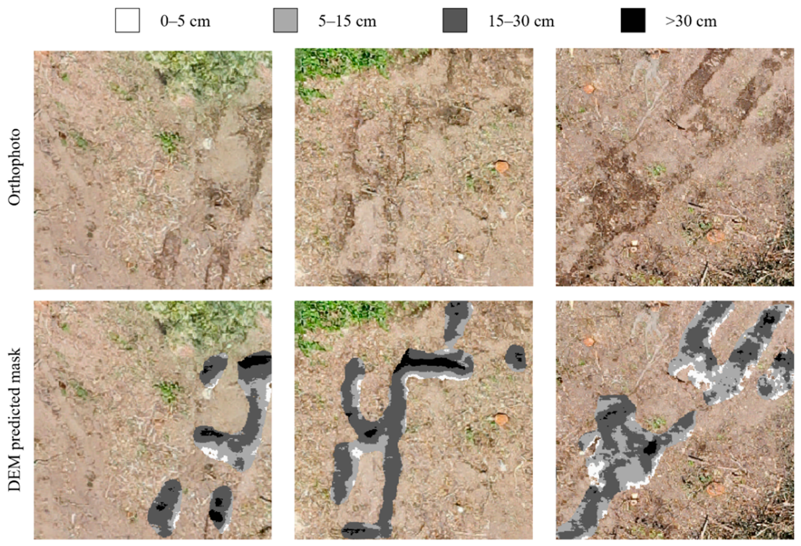
To enable a comparison with field-based visual assessments, the detected rut areas were further classified according to the disturbance severity scheme proposed by McMahon [46]. The McMahon classification system is a ground-based field survey method originally developed to assess soil disturbance severity in forest harvesting operations, in which disturbance types are assigned numerical codes based on observable surface conditions such as litter displacement, topsoil exposure, puddling, and rutting depth. This classification system has been applied in various forestry studies as a standardized framework for characterizing machine-induced soil disturbance [19,47,48]. Specifically, rut pixels with a calculated relative depth (D) exceeding 5 cm, corresponding to the threshold defined for rutting disturbances (code 9 and above) in the McMahon classification system, were retained for classification. These pixels were subsequently subdivided into three depth categories: shallow rutting (5–15 cm; code 9), moderate rutting (15–30 cm; code 10), and deep rutting (>30 cm; code 11). Pixels with D < 5 cm, identified as soil disturbances by the segmentation model, were excluded from the rutting-depth classification because they were below the minimum rutting threshold. The areal extent of each depth class was calculated by summing the corresponding pixel counts and multiplying them by the pixel area derived from the UAV-based DEM resolution.
2.6. Field Validation
The manual pinboard method was employed to measure the actual soil surface deformation caused by the machine traffic [24]. The pinboard was 80 cm in width and 30 cm in length, exceeding the width of typical forestry machine crawler tracks. The board was equipped with a leveling device to ensure horizontal alignment during the measurements. Grid lines at 1 cm intervals were marked on the board surface, and 70 steel pins (diameter: 1 mm) were installed at a spacing of 1 cm. The pins were freely movable, allowing their tips to make direct contact with the soil surface, and the upper ends were marked with colored tape to facilitate visual reading.
Pinboard measurements were conducted from 18 June 2023 to 20 June 2023, concurrent with UAV data acquisition. Measurement locations (n = 38) were selected to represent accessible areas with visible disturbances, while maintaining spatial distribution across the study site.
The vertical displacement profile of the soil surface was recorded at each location. Based on the measured profile, the maximum rut depth was identified as the deepest vertical depression relative to the surrounding undisturbed surface. Profile photographs were captured using a 1 cm reference scale for documentation.
To evaluate the accuracy of DEM-based depth estimation, a circular buffer with a radius of 0.30 m was generated around each pinboard measurement location. This buffer size accounted for the crawler width (0.38 m) and GPS positioning uncertainty. Within each buffer, the maximum DEM-estimated depth was calculated and compared to the corresponding pinboard-measured maximum depth. In addition, a field location was considered successfully detected when at least one raster pixel with a DEM-derived depth ≥ 5 cm occurred within the buffer.
2.7. Statistical Analysis
Model performance metrics (IoU, F1-score, precision, recall, and accuracy) were calculated for each cross-validation fold and reported as mean ± standard deviation across five folds.
For field validation, Spearman’s rank correlation coefficient was used to assess the relationship between the DEM-estimated and pinboard-measured depths owing to potential nonlinear relationships. The RMSE was calculated to quantify the depth estimation accuracy. Statistical significance was evaluated at α = 0.05.
All analyses were performed using R software 4.3.1 and Python 3.9.13.
3. Results
3.1. CNN-Based Soil Disturbance Detection Performance
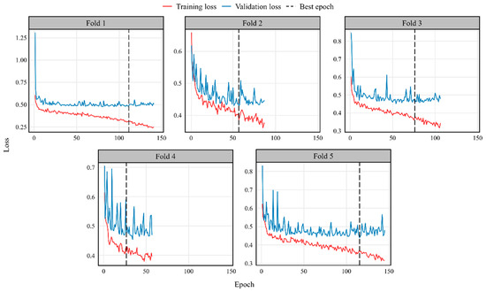
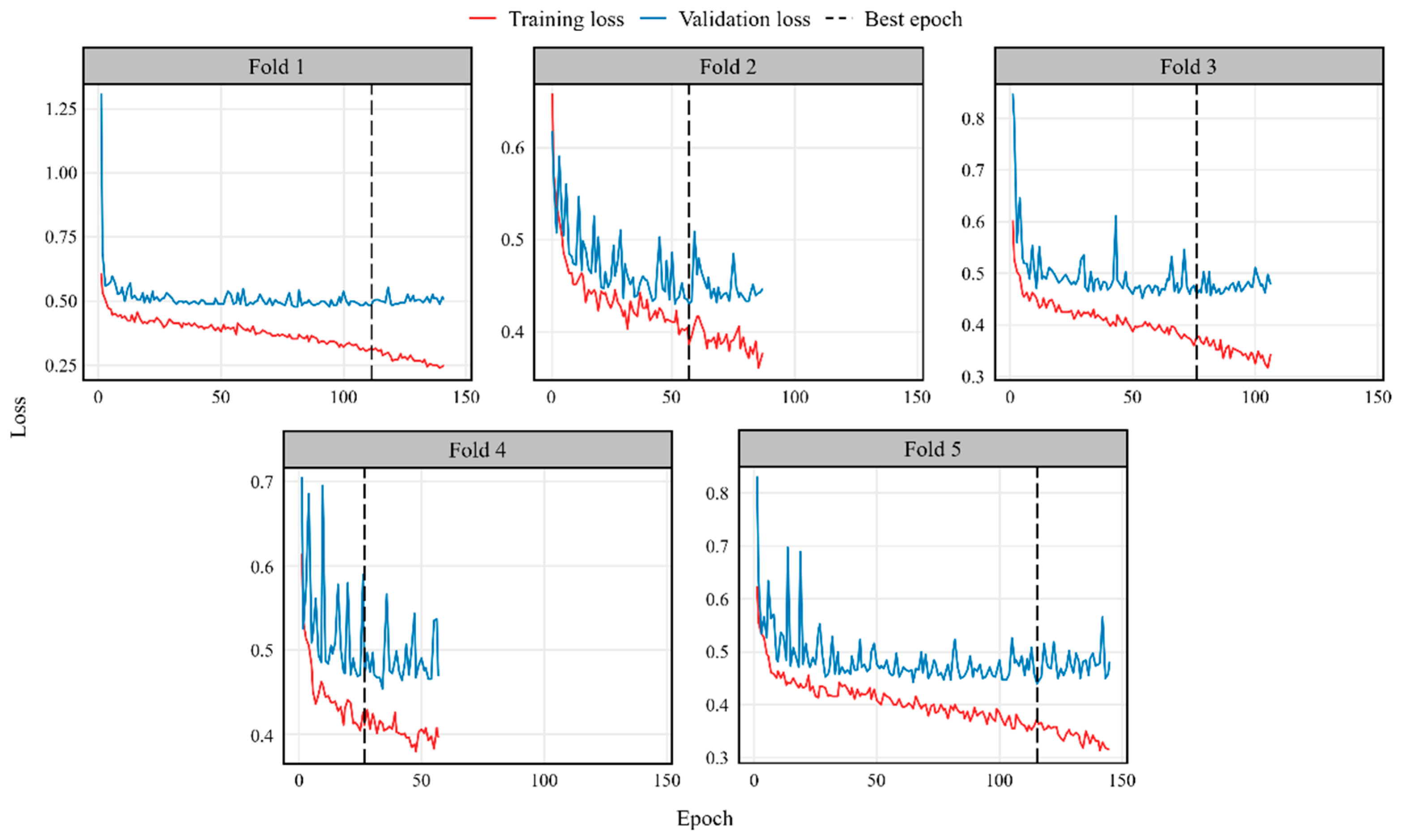
All five cross-validation folds converged with the best epochs at 111, 57, 76, 27, and 115 for folds 1–5 (Figure 3). The training and validation losses generally decreased across all folds, with the validation loss showing fold-dependent variability before stabilizing near convergence. The fold-dependent variability observed in the validation loss curves is likely related to differences in the spatial composition of each validation fold, as the proportion of disturbance pixels ranged from 4.67% to 8.72% across folds. Validation IoU at best epoch ranged from 0.3513 to 0.4720 (mean: 0.4194 ± 0.0527). The performance of the test set across the five folds is presented in Table 2. The mean IoU was 0.4138 ± 0.0133, and F1-score was 0.5853 ± 0.0133, with precision of 0.5451 ± 0.0273 and recall of 0.6334 ± 0.0180. Precision was consistently lower than recall across all folds, indicating a higher rate of false positive predictions relative to false negatives.
Figure 3.
Training and validation loss curves for five cross-validation folds. Red lines, training loss; Blue lines, validation loss; Dashed vertical lines, best epoch.
Table 2.
Five-fold cross-validation results of the U-Net model for soil disturbance segmentation.
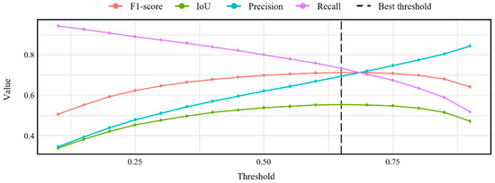
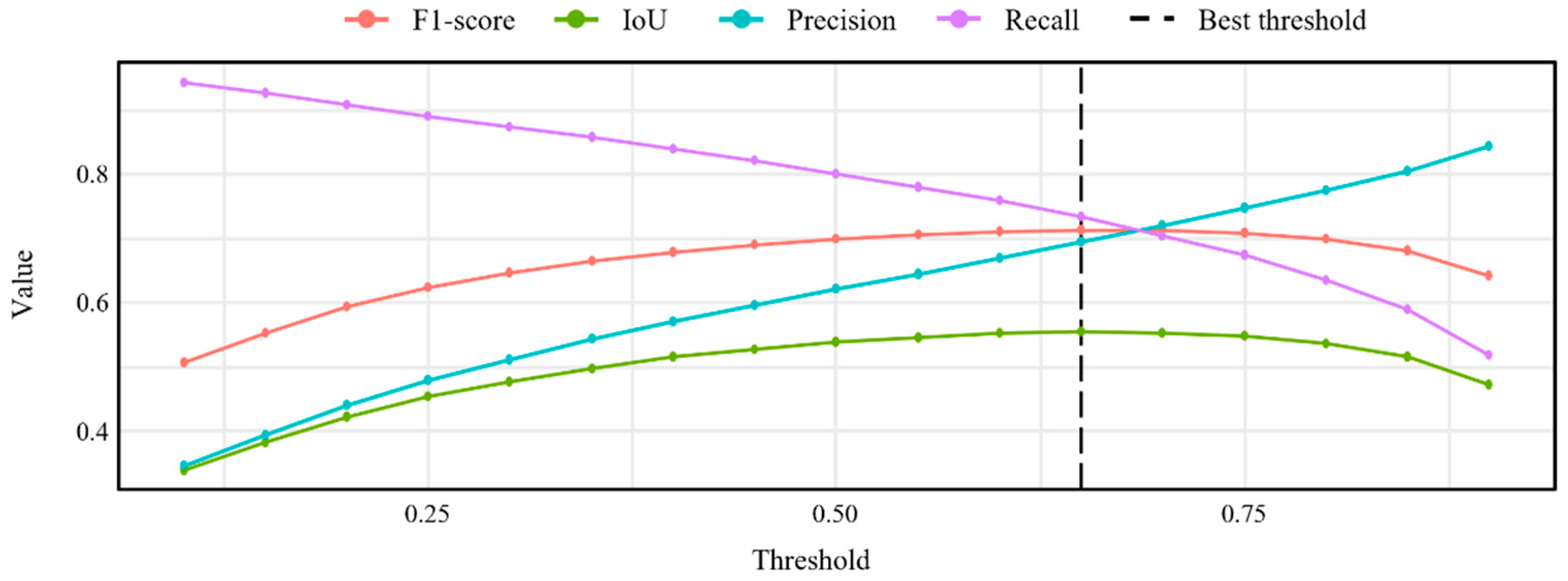
The ensemble threshold optimization identified 0.65 as the optimal threshold, which achieved an F1-score of 0.7130, IoU of 0.5540, precision of 0.6941, and recall of 0.7330 (Figure 4). Threshold sensitivity analysis across the range 0.10–0.90 showed a typical precision-recall trade-off, with precision increasing from 0.3449 to 0.8447 and recall decreasing from 0.9441 to 0.5175. The F1-score remained stable above 0.70 across thresholds ranging from 0.55 to 0.75.
Figure 4.
Variation in performance metrics across probability thresholds.
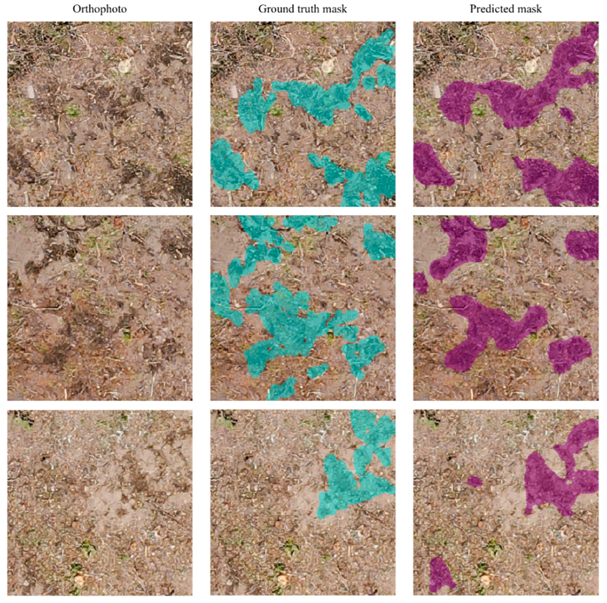
At a threshold of 0.65, the CNN detection identified 0.186 ha (7.44% of the site). Representative examples (Figure 5) showed strong spatial agreement between ground truth (cyan) and predictions (purple), with discrepancies mainly at patch edges where annotation boundaries were ambiguous.
Figure 5.
Visual comparison of orthophoto, ground truth mask, and predicted soil disturbance mask.
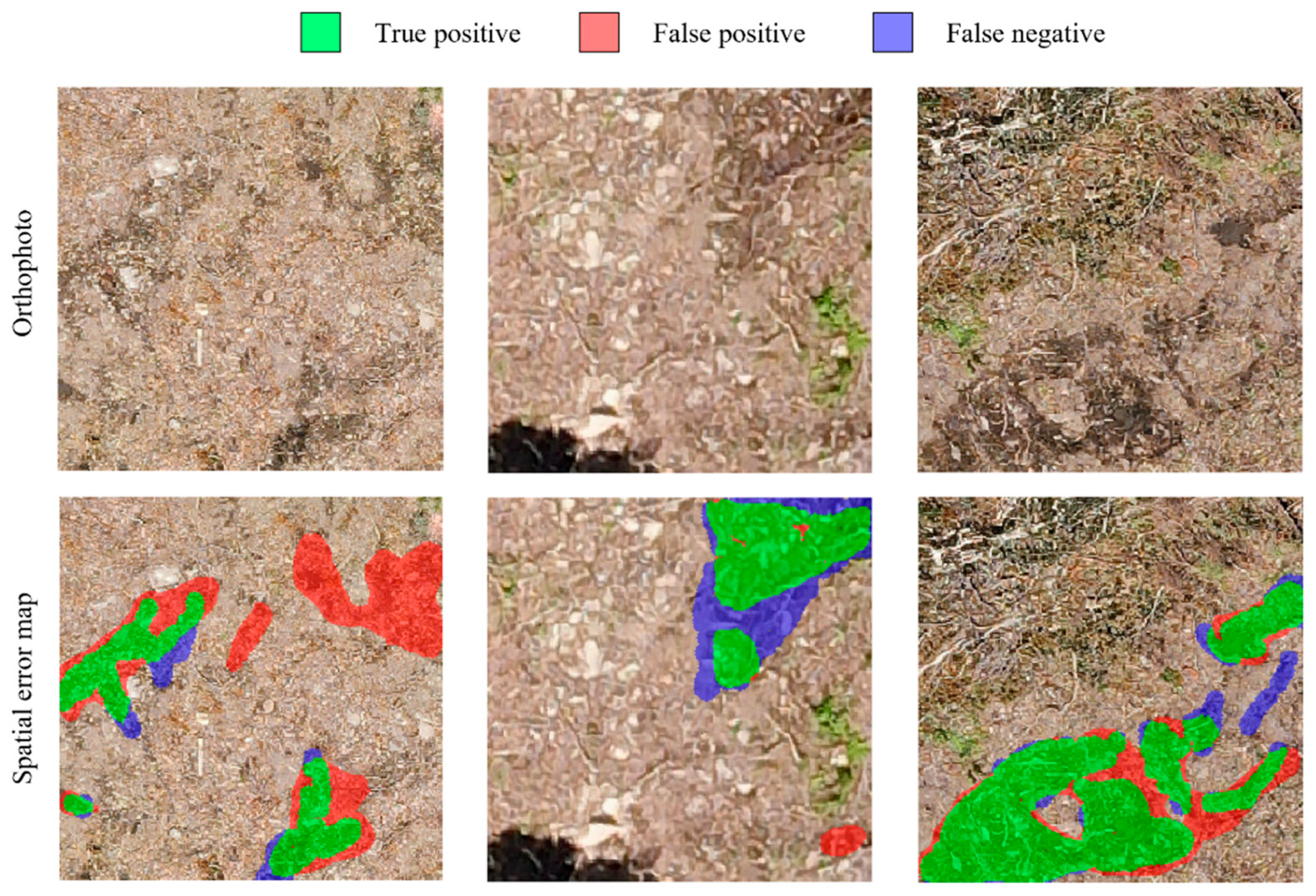
To further characterize the spatial distribution of prediction errors, spatial error maps were generated by classifying each pixel into TP (green), FP (red), and FN (blue) categories at the ensemble threshold of 0.65 (Figure 6). FP errors were predominantly observed in areas exhibiting spectral characteristics similar to disturbed surfaces. FN errors were concentrated primarily at the boundaries of disturbance patches (FN rate: 48.5%) compared to patch interiors (FN rate: 24.0%), where annotation boundaries were inherently ambiguous.
Figure 6.
Representative examples of spatial prediction errors overlaid on orthophotos.
3.2. DEM-Based Depth Estimation and Severity Classification
DEM-based depth estimation was successfully applied to 96.4% of the CNN-detected pixels (0.180 of 0.186 ha). Estimated depths ranged from 0 to 36.5 cm, with a mean depth of 15.3 ± 8.2 cm across all analyzed pixels. Based on the full depth distribution of all analyzed pixels, 12.7% were <5 cm, 53.0% were within 5–15 cm, 31.9% were within 15–30 cm, and 2.4% exceeded 30 cm (Table 3).
Table 3.
Area distribution of soil disturbance severity classes based on DEM-derived depth estimation.
The application of the 5 cm depth threshold excluded pixels representing shallow surface alterations, reducing the classified disturbance area by 15.6% from 0.180 to 0.157 ha. The excluded pixels (0.023 ha) represented detectable surface changes that were below the functional threshold for significant soil rutting.
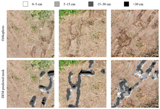
Among the retained disturbances (≥5 cm), severity was redistributed as follows: light disturbances (5–15 cm) comprised 0.095 ha (60.7% of the ≥5 cm area; 3.80% of the total site), moderate disturbances (15–30 cm) accounted for 0.057 ha (36.5%; 2.29% of site), and severe disturbances (>30 cm) represented 0.004 ha (2.8%; 0.17% of site; Table 3). Representative examples of the spatial distribution of severity classes across the study sites are shown in Figure 7.
Figure 7.
Examples of DEM-based soil disturbance severity classification overlaid on orthophotos.
3.3. Field Validation
The field-measured maximum rut depths ranged from 8.2 to 30.6 cm (mean: 19.8 ± 4.9 cm), with all measurement locations substantially exceeding the 5 cm threshold used to define significant soil disturbance, consistent with the visible rutting criteria applied during field site selection.
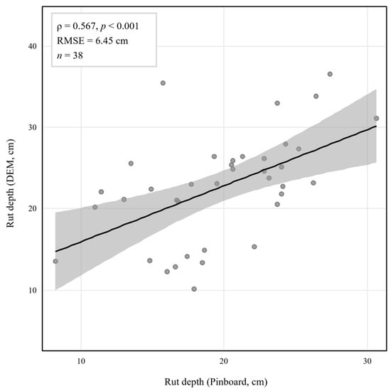
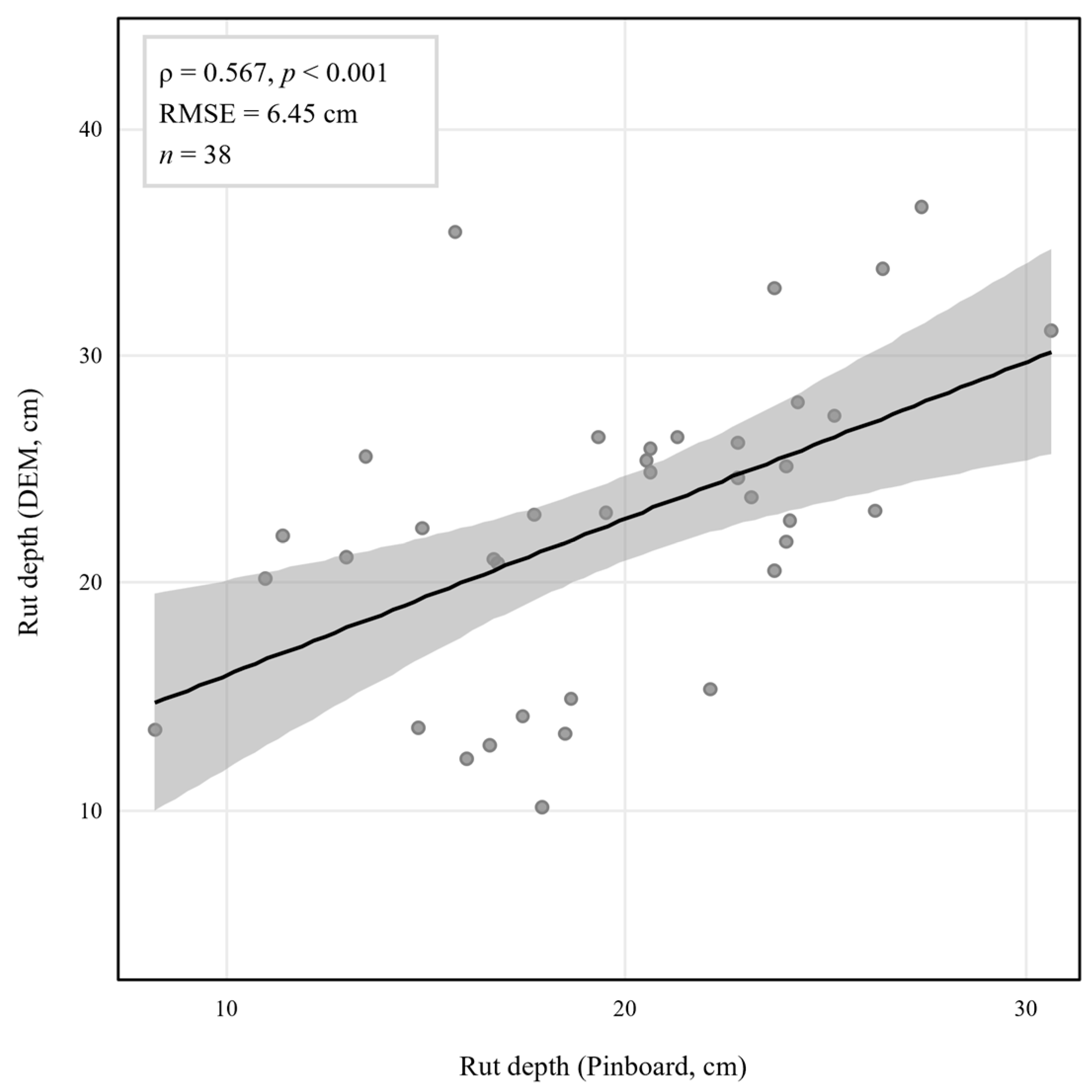
Quantitative comparison of rut depth magnitude showed a moderately positive correlation between field-measured maximum rut depth and DEM-derived maximum depth within the 0.30 m buffer (ρ = 0.567, p < 0.001; n = 38; Figure 8), with RMSE of 6.45 cm.
Figure 8.
Relationship between field-measured and DEM-derived rut depth.
4. Discussion
The U-Net model achieved a mean test IoU of 0.4138 and an F1-score of 0.5853 across five cross-validation folds. These values are comparatively lower than segmentation and detection performances reported in other forestry remote sensing applications, where F1-scores of 0.77–0.87 have been reported for tasks such as individual tree detection [35,49], logging trail segmentation [50], and forest disturbance mapping [51], with IoU reaching 0.867 for logging trail detection under controlled stand conditions [50]. The most directly comparable study, Bhatnagar et al. [37], reported a mean F1-score of 0.77 for wheel-rut mapping from drone imagery across 20 harvested sites under varying terrain conditions. While CNN-based approaches have been increasingly adopted for various forestry remote sensing tasks, their application to mapping harvesting-induced disturbances in steep-slope harvesting environments has not been widely explored, and the present study represents an early attempt to address this gap in steep-slope environments.
The comparatively lower performance observed in the present study is attributable to the substantially more challenging application context, as machine-induced soil disturbances in steep forest terrain are characterized by irregular morphology and transitional boundaries that are difficult to delineate consistently, even among human annotators [37,52], unlike the well-defined targets typical of agricultural [53] or urban [54] segmentation tasks. Spatial error analysis confirmed these patterns: FN errors were disproportionately concentrated at disturbance patch boundaries (FN rate: 48.5%) compared to patch interiors (FN rate: 24.0%), reflecting the inherent difficulty of delineating transitional boundary regions, while FP errors were predominantly observed in spectrally ambiguous areas arising from shadow effects caused by steep terrain and residual canopy cover. The incorporation of DEM-assisted weak labels during training may have further introduced uncertain boundary regions into the learning process.
The fold-dependent variability in validation loss is attributable to the inherent spatial clustering of soil disturbance, which resulted in uneven disturbance pixel distributions across folds despite block-based spatial partitioning. At the ensemble level, predictions at an optimized threshold of 0.65 achieved an F1-score of 0.7130 and IoU of 0.5540, with performance maintained within a moderate threshold range, suggesting some flexibility in threshold selection depending on management objectives.
However, two methodological choices warrant further discussion. The incremental contribution of the DEM relative to the RGB input has not been formally evaluated, and future ablation experiments are needed to quantify the added value of the topographic information. Regarding the differential weighting scheme, the absence of a formal sensitivity analysis means that the degree of uncertainty introduced by this parameter choice cannot be fully quantified. In this study, soil disturbances were identified through visually distinct surface signatures in RGB imagery, whereas DEM-based identification relied on microtopographic depression (Figure 1). Because these two modalities capture different aspects of disturbance expression, assigning higher weights to DEM-identified regions may introduce systematic bias in the predicted disturbance area, as modalities with varying predictive power and noise topology can produce imbalanced contributions during fusion [55]. This parameter uncertainty has implications for the reproducibility and transferability of the approach, and systematic sensitivity analysis is recommended as part of model calibration when adapting this framework to new contexts.
DEM-based depth estimation successfully quantified rut severity for 96.4% of detected pixels, with most disturbances classified as light (53.0% in the 5–15 cm range) or moderate (31.9% in the 15–30 cm range), consistent with the operational constraints of excavator-based harvesting on steep terrain [22,56]. Depth-based filtering reduced the mapped disturbance area from 0.186 to 0.157 ha (15.6%), excluding shallow surface alterations that may otherwise be misinterpreted as functionally significant soil degradation [57]. The detected disturbance proportions were within ranges reported for ground-based harvesting systems, though at the lower end [58,59], which is likely attributable to the steep slope restricting machine movement to selected travel corridors, the log-throwing extraction method reducing lateral soil disturbance, and the 5 cm threshold excluding shallow alterations counted in binary presence/absence assessments. Given the RMSE of 6.45 cm in DEM-derived depth estimates, some misclassification between adjacent severity classes cannot be excluded, particularly near the 5 cm and 15 cm class boundaries. However, as the majority of detected disturbances fell well within the light (53.0%) and moderate (31.9%) categories with depth ranges substantially exceeding the class boundaries, the overall severity distribution is unlikely to be fundamentally altered by this uncertainty, and the proportional patterns reported here are considered broadly representative of the disturbance conditions at the study site.
All 38 field-measured disturbance locations were identified within 0.30 m buffers, demonstrating reliable spatial detection. An RMSE of 6.45 cm and a moderate correlation (ρ = 0.567) between DEM estimates and pinboard measurements indicate that absolute depth prediction exhibits variability at individual points; however, it remains effective for characterizing relative severity. These results are broadly consistent with comparable UAV-based rut depth validation studies; Nevalainen et al. [60] reported a Pearson correlation of r = 0.67, while Büyüksakallı et al. [61] reported r = 0.850 under flat to gently sloping terrain, with the lower correlation in the present study likely reflecting the steeper terrain and single-epoch DEM approach. Contributing error sources include DEM resolution limitations, GPS positioning uncertainty, and operator-induced variability in pinboard measurements.
It should also be noted that independent DEM vertical accuracy validation against ground control points was not conducted. However, the pinboard-based comparison provides an indirect assessment of relative elevation accuracy within disturbance areas, which is most directly relevant to the severity classification objective. Furthermore, the field validation dataset of 38 measurements, while representative of accessible disturbance locations across the study site, represents a relatively small sample for robust statistical validation; the observed correlation and RMSE should therefore be interpreted with caution, and expanded field sampling using a stratified design is recommended in future studies. Finally, manual annotations represent post hoc interpretations of visible disturbance signatures rather than absolute ground truths [62], and the reported disturbance proportions should therefore be interpreted as empirically observed visible disturbance under operational conditions, rather than a deviation from a known true baseline.
The soil disturbances are likely to have implications beyond immediate physical impacts, as compaction and rutting in harvested areas have been associated with altered carbon dynamics, hydrological processes, and forest regeneration potential [63,64,65]. While these broader ecosystem effects were not directly assessed here, spatially explicit disturbance maps may provide a useful basis for future studies linking harvesting impacts to ecosystem-level outcomes relevant to sustainable forest management.
As this study was conducted at a single site, the model performance under different soil types, vegetation conditions, illumination conditions, equipment configurations, and terrain complexity conditions remains uncertain, and cross-site validation is essential for assessing the generalization capacity. Future research should focus on (1) multi-site validation to establish generalization capabilities and calibration requirements; (2) expanding field sampling using a stratified design that ensures adequate representation across all severity classes; (3) systematic comparisons of depth estimation methods, such as multitemporal DEM differencing and machine learning-based approaches; (4) ablation studies to quantify the contribution of DEM and RGB input channels; and (5) systematic comparison of alternative model architectures, including U-Net variants with pretrained encoders and other segmentation frameworks such as DeepLabv3+.
5. Conclusions
Our hypothesis that integrating UAV-derived high-resolution imagery with CNN-based semantic segmentation can provide accurate and scalable detection of soil disturbance and its severity in steep-slope harvesting environments was partially supported. While reliable spatial detection and meaningful severity classification were demonstrated, the limited segmentation performance and depth estimation error indicate that further refinement is needed before operational deployment.
DEM-derived depth estimation enabled severity classification, with light disturbances predominating and moderate to severe cases being progressively less frequent, reflecting the operational constraints of excavator-based harvesting on steep slopes. Field validation demonstrated the reliable spatial detection of disturbance locations, although absolute depth prediction exhibited the expected variability owing to microtopographic complexity. However, the generalizability of the proposed approach remains to be validated across diverse sites, soil types, and harvesting operation types.
In conclusion, CNN-based semantic segmentation applied to high-resolution UAV imagery shows potential as a viable approach for automated disturbance mapping in steep-slope forestry where traditional monitoring encounters fundamental constraints. This framework may support environmentally responsible forest management practices in mountainous regions by providing spatially comprehensive and objectively quantified assessment capabilities. With continued improvements in model generalizability and DEM accuracy, its integration into post-harvest assessment could support evidence-based decisions that balance environmental protection and sustainable timber production.
Author Contributions
Conceptualization, B.C. and I.K.; methodology, I.K.; software, I.K. and J.S.; validation, B.C., I.K. and J.S.; formal analysis, I.K. and J.S.; investigation, I.K. and J.S.; resources, B.C.; data curation, J.S.; writing—original draft preparation, J.S.; writing—review and editing, I.K. and B.C.; visualization, J.S.; supervision, B.C.; project administration, B.C.; funding acquisition, B.C. All authors have read and agreed to the published version of the manuscript.
Funding
This research was supported by the National Research Foundation of Korea (NRF) funded by the Korean government (No. NRF-2021R1A2C2008002).
Data Availability Statement
The data presented in this study are available on reasonable request from the corresponding author. Data related to the study have been presented within the article.
Conflicts of Interest
The authors declare that they have no competing financial interests related to personal relationships that could have influenced the work reported in this study.
References
- Axelsson, S.Å. The mechanization of logging operations in Sweden and its effect on occupational safety and health. J. For. Eng. 1998, 9, 25–31. [Google Scholar] [CrossRef] [Scilit]
- Yoshimura, T.; Suzuki, Y.; Sato, N. Assessing the productivity of forest harvesting systems using a combination of forestry machines in steep terrain. Forests 2023, 14, 1430. [Google Scholar] [CrossRef] [Scilit]
- Medvedev, V.V.; Cybulko, W.G. Soil criteria for assessing the maximum permissible ground pressure of agricultural vehicles on Chernozem soils. Soil Tillage Res. 1995, 36, 153–164. [Google Scholar] [CrossRef] [Scilit]
- Horn, R.; Vossbrink, J.; Becker, S. Modern forestry vehicles and their impacts on soil physical properties. Soil Tillage Res. 2004, 79, 207–219. [Google Scholar] [CrossRef] [Scilit]
- Labelle, E.R.; Jaeger, D. Soil compaction caused by cut-to-length forest operations and possible short-term natural rehabilitation of soil density. Soil Sci. Soc. Am. J. 2011, 75, 2314–2329. [Google Scholar] [CrossRef] [Scilit]
- Kormanek, M.; Dvořák, J. Ground pressure changes caused by MHT 8002HV crawler harvester chassis. Croat. J. For. Eng. 2021, 42, 201–211. [Google Scholar] [CrossRef] [Scilit]
- McNabb, D.H.; Startsev, A.D.; Nguyen, H. Soil wetness and traffic level effects on bulk density and air-filled porosity of compacted boreal forest soils. Soil Sci. Soc. Am. J. 2001, 65, 1238–1247. [Google Scholar] [CrossRef] [Scilit]
- Kremers, J.; Boosten, M. Soil Compaction and Deformation in Forest Exploitation. A Literature Review on Causes and Effects and Guidelines on Avoiding Compaction and Deformation; Stichting Probos: Wageningen, The Netherlands, 2018; Available online: https://www.probos.nl/images/pdf/rapporten/Rap2018_soil_compaction_and_deformation_in_forest_exploitation.pdf (accessed on 23 March 2026).
- Cambi, M.; Certini, G.; Neri, F.; Marchi, E. The impact of heavy traffic on forest soils: A review. For. Ecol. Manag. 2015, 338, 124–138. [Google Scholar] [CrossRef] [Scilit]
- Kozlowski, T.T. Soil compaction and growth of woody plants. Scand. J. For. Res. 1999, 14, 596–619. [Google Scholar] [CrossRef]
- Startsev, A.D.; McNabb, D.H. Effects of compaction on aeration and morphology of boreal forest soils in Alberta, Canada. Can. J. Soil Sci. 2009, 89, 45–56. [Google Scholar] [CrossRef] [Scilit]
- Watson, G.W.; Kelsey, P. The impact of soil compaction on soil aeration and fine root density of Quercus palustris. Urban For. Urban Green. 2006, 4, 69–74. [Google Scholar] [CrossRef] [Scilit]
- Froehlich, H.A.; Miles, D.W.R.; Robbins, R.W. Soil bulk density recovery on compacted skid trails in central Idaho. Soil Sci. Soc. Am. J. 1985, 49, 1015–1017. [Google Scholar] [CrossRef] [Scilit]
- Powers, R.F.; Scott, D.A.; Sanchez, F.G.; Voldseth, R.A.; Page-Dumroese, D.; Elioff, J.D.; Stone, D.M. The North American long-term soil productivity experiment: Findings from the first decade of research. For. Ecol. Manag. 2005, 220, 31–50. [Google Scholar] [CrossRef] [Scilit]
- Hartmann, M.; Howes, C.G.; VanInsberghe, D.; Yu, H.; Bachar, D.; Christen, R.; Nilsson, R.H.; Hallam, S.J.; Mohn, W.W. Significant and persistent impact of timber harvesting on soil microbial communities in northern coniferous forests. ISME J. 2012, 6, 2199–2218. [Google Scholar] [CrossRef] [Scilit] [PubMed]
- Lewandowski, T.E.; Forrester, J.A.; Mladenoff, D.J.; Marin-Spiotta, E.; D’Amato, A.W.; Palik, B.J.; Kolka, R.K. Long term effects of intensive biomass harvesting and compaction on the forest soil ecosystem. Soil Biol. Biochem. 2019, 137, 107572. [Google Scholar] [CrossRef] [Scilit]
- Ball, B.C.; Scott, A.; Parker, J.P. Field N2O, CO2 and CH4 fluxes in relation to tillage, compaction and soil quality in Scotland. Soil Tillage Res. 1999, 53, 29–39. [Google Scholar] [CrossRef] [Scilit]
- Smith, K.A.; Ball, T.; Conen, F.; Dobbie, K.E.; Massheder, J.; Rey, A. Exchange of greenhouse gases between soil and atmosphere: Interactions of soil physical factors and biological processes. Eur. J. Soil Sci. 2018, 69, 10–20. [Google Scholar] [CrossRef] [Scilit]
- Allman, M.; Jankovský, M.; Messingerová, V.; Allmanová, Z. Soil moisture content as a predictor of soil disturbance caused by wheeled forest harvesting machines on soils of the Western Carpathians. J. For. Res. 2017, 28, 283–289. [Google Scholar] [CrossRef] [Scilit]
- Wood, M.J.; Carling, P.A.; Moffat, A.J. Reduced ground disturbance during mechanized forest harvesting on sensitive forest soils in the UK. Forestry 2003, 76, 345–361. [Google Scholar] [CrossRef] [Scilit]
- Ampoorter, E.; Goris, R.; Cornelis, W.M.; Verheyen, K. Impact of mechanized logging on compaction status of sandy forest soils. For. Ecol. Manag. 2007, 241, 162–174. [Google Scholar] [CrossRef] [Scilit]
- Visser, R.; Stampfer, K. Expanding ground-based harvesting onto steep terrain: A review. Croat. J. For. Eng. 2015, 36, 321–331. [Google Scholar]
- Eliasson, L.; Wästerlund, I. Effects of slash reinforcement of strip roads on rutting and soil compaction on a moist fine-grained soil. For. Ecol. Manag. 2007, 252, 118–123. [Google Scholar] [CrossRef] [Scilit]
- Kuipers, H. A reliefmeter for soil cultivation studies. Neth. J. Agric. Sci. 1957, 5, 255–262. [Google Scholar] [CrossRef] [Scilit]
- Saleh, A. Soil roughness measurement: Chain method. J. Soil Water Conserv. 1993, 48, 527–529. [Google Scholar] [CrossRef] [Scilit]
- Jester, W.; Klik, A. Soil surface roughness measurement—Methods, applicability, and surface representation. CATENA 2005, 64, 174–192. [Google Scholar] [CrossRef] [Scilit]
- Giannetti, F.; Chirici, G.; Travaglini, D.; Bottalico, F.; Marchi, E.; Cambi, M. Assessment of soil disturbance caused by forest operations by means of portable laser scanner and soil physical parameters. Soil Sci. Soc. Am. J. 2017, 81, 1577–1585. [Google Scholar] [CrossRef] [Scilit]
- Talbot, B.; Rahlf, J.; Astrup, R. An operational UAV-based approach for stand-level assessment of soil disturbance after forest harvesting. Scand. J. For. Res. 2018, 33, 387–396. [Google Scholar] [CrossRef] [Scilit]
- Koren, M.; Slančík, M.; Suchomel, J.; Dubina, J. Use of terrestrial laser scanning to evaluate the spatial distribution of soil disturbance by skidding operations. iForest 2015, 8, 386. [Google Scholar] [CrossRef] [Scilit]
- Krause, S.; Sanders, T.G.; Mund, J.P.; Greve, K. UAV-based photogrammetric tree height measurement for intensive forest monitoring. Remote Sens. 2019, 11, 758. [Google Scholar] [CrossRef] [Scilit]
- Westoby, M.J.; Brasington, J.; Glasser, N.F.; Hambrey, M.J.; Reynolds, J.M. Structure-from-Motion photogrammetry: A low-cost, effective tool for geoscience applications. Geomorphology 2012, 179, 300–314. [Google Scholar] [CrossRef] [Scilit]
- Maltamo, M.; Næsset, E.; Vauhkonen, J. Forestry Applications of Airborne Laser Scanning: Concepts and Case Studies; Springer: Dordrecht, The Netherlands, 2014; Volume 27. [Google Scholar]
- Zhu, X.X.; Tuia, D.; Mou, L.; Xia, G.S.; Zhang, L.; Xu, F.; Fraundorfer, F. Deep learning in remote sensing: A comprehensive review and list of resources. IEEE Geosci. Remote Sens. Mag. 2017, 5, 8–36. [Google Scholar] [CrossRef] [Scilit]
- Belgiu, M.; Drăguţ, L. Random forest in remote sensing: A review of applications and future directions. ISPRS J. Photogramm. Remote Sens. 2016, 114, 24–31. [Google Scholar] [CrossRef] [Scilit]
- Weinstein, B.G.; Marconi, S.; Bohlman, S.; Zare, A.; White, E. Individual tree-crown detection in RGB imagery using semi-supervised deep learning neural networks. Remote Sens. 2019, 11, 1309. [Google Scholar] [CrossRef] [Scilit]
- Zheng, S.; Zou, X.; Gao, P.; Zhang, Q.; Hu, F.; Zhou, Y.; Wu, Z.; Wang, W.; Chen, S. A forest fire recognition method based on modified deep CNN model. Forests 2024, 15, 111. [Google Scholar] [CrossRef] [Scilit]
- Bhatnagar, S.; Puliti, S.; Talbot, B.; Heppelmann, J.B.; Breidenbach, J.; Astrup, R. Mapping wheel-ruts from timber harvesting operations using deep learning techniques in drone imagery. Forestry 2022, 95, 698–710. [Google Scholar] [CrossRef] [Scilit]
- Köppen, W. Das Geographische System der Klimate; Gebrüder Borntraeger: Berlin, Germany, 1936. [Google Scholar]
- Soil Survey Staff. Keys to Soil Taxonomy, 12th ed.; USDA-Natural Resources Conservation Service: Washington, DC, USA, 2014. [Google Scholar]
- Latterini, F.; Venanzi, R.; Tocci, D.; Moschetti, F.; Picchio, R. Comparing accuracy of three remote sensing methods to evaluate soil impact related to forest operations. Environ. Sci. Proc. 2020, 3, 59. [Google Scholar]
- Ronneberger, O.; Fischer, P.; Brox, T. U-Net: Convolutional networks for biomedical image segmentation. In Proceedings of the International Conference on Medical Image Computing and Computer-Assisted Intervention (MICCAI 2015), Munich, Germany, 5–9 October 2015; Springer: Cham, Switzerland, 2015; pp. 234–241. [Google Scholar]
- Bressan, P.O.; Junior, J.M.; Martins, J.A.C.; de Melo, M.J.; Gonçalves, D.N.; Freitas, D.M.; Ramos, A.P.M.; Furuya, M.T.G.; Osco, L.P.; de Andrade Silva, J.; et al. Semantic segmentation with labeling uncertainty and class imbalance applied to vegetation mapping. Int. J. Appl. Earth Obs. Geoinf. 2022, 108, 102690. [Google Scholar] [CrossRef] [Scilit]
- Kang, S.H.; Kim, K.; Shim, J.; Lee, Y. Feasibility of U-Net model for cerebral arteries segmentation with low-dose computed tomography angiographic images with pre-processing methods. Sci. Rep. 2025, 15, 13281. [Google Scholar] [CrossRef] [Scilit] [PubMed]
- Sokolova, M.; Lapalme, G. A systematic analysis of performance measures for classification tasks. Inf. Process. Manag. 2009, 45, 427–437. [Google Scholar] [CrossRef] [Scilit]
- Nurunnabi, A.; Belton, D.; West, G. Robust statistical approaches for local planar surface fitting in 3D laser scanning data. ISPRS J. Photogramm. Remote Sens. 2014, 96, 106–122. [Google Scholar] [CrossRef] [Scilit]
- McMahon, S. Accuracy of two ground survey methods for assessing site disturbance. J. For. Eng. 1995, 6, 27–33. [Google Scholar] [CrossRef] [Scilit]
- Naghdi, R.; Solgi, A.; Zenner, E.K. Soil disturbance caused by different skidding methods in mountainous forests of Northern Iran. Int. J. For. Eng. 2015, 26, 212–224. [Google Scholar] [CrossRef] [Scilit]
- Lee, E.; Eu, S.; Li, Q. Assessment of soil erosion potential from the disturbed surface of skid trails in small shovel harvesting system. Front. Environ. Sci. 2022, 10, 756848. [Google Scholar] [CrossRef] [Scilit]
- Mohan, M.; Silva, C.A.; Klauberg, C.; Jat, P.; Catts, G.; Cardil, A.; Hudak, A.T.; Dia, M. Individual tree detection from unmanned aerial vehicle (UAV) derived canopy height model in an open canopy mixed conifer forest. Forests 2017, 8, 340. [Google Scholar] [CrossRef] [Scilit]
- Abdi, O.; Uusitalo, J.; Kivinen, V.P. Logging trail segmentation via a novel U-net convolutional neural network and high-density laser scanning data. Remote Sens. 2022, 14, 349. [Google Scholar] [CrossRef] [Scilit]
- Kislov, D.E.; Korznikov, K.A.; Altman, J.; Vozmishcheva, A.S.; Krestov, P.V. Extending deep learning approaches for forest disturbance segmentation on very high-resolution satellite images. Remote Sens. Ecol. Conserv. 2021, 7, 355–368. [Google Scholar] [CrossRef] [Scilit]
- Martin, D.; Fowlkes, C.; Tal, D.; Malik, J. A database of human segmented natural images and its application to evaluating segmentation algorithms and measuring ecological statistics. In Proceedings of the Eighth IEEE International Conference on Computer Vision (ICCV 2001), Vancouver, BC, Canada, 7–14 July 2001; IEEE: Piscataway, NJ, USA, 2001; Volume 2, pp. 416–423. [Google Scholar]
- Kamilaris, A.; Prenafeta-Boldú, F.X. A review of the use of convolutional neural networks in agriculture. J. Agric. Sci. 2018, 156, 312–322. [Google Scholar] [CrossRef] [Scilit]
- Marmanis, D.; Wegner, J.D.; Galliani, S.; Schindler, K.; Datcu, M.; Stilla, U. Semantic segmentation of aerial images with an ensemble of CNNs. ISPRS Ann. Photogramm. Remote Sens. Spat. Inf. Sci. 2016, 3, 473–480. [Google Scholar]
- Baltrušaitis, T.; Ahuja, C.; Morency, L.-P. Multimodal Machine Learning: A Survey and Taxonomy. IEEE Trans. Pattern Anal. Mach. Intell. 2019, 41, 423–443. [Google Scholar] [CrossRef] [Scilit] [PubMed]
- Cavalli, R.; Amishev, D. Steep terrain forest operations—Challenges, technology development, current implementation, and future opportunities. Int. J. For. Eng. 2019, 30, 175–181. [Google Scholar] [CrossRef] [Scilit]
- Curran, M.P.; Miller, R.E.; Howes, S.W.; Maynard, D.G.; Terry, T.A.; Heninger, R.L.; Niemann, T.; Van Rees, K.; Powers, R.F.; Schoenholtz, S.H. Progress towards more uniform assessment and reporting of soil disturbance for operations, research, and sustainability protocols. For. Ecol. Manag. 2005, 220, 17–30. [Google Scholar] [CrossRef] [Scilit]
- Zenner, E.K.; Fauskee, J.T.; Berger, A.L.; Puettmann, K.J. Impacts of skidding traffic intensity on soil disturbance, soil recovery, and aspen regeneration in north central Minnesota. North. J. Appl. For. 2007, 24, 177–183. [Google Scholar] [CrossRef] [Scilit]
- Reeves, D.A.; Reeves, M.C.; Abbott, A.M.; Page-Dumroese, D.S.; Coleman, M.D. A detrimental soil disturbance prediction model for ground-based timber harvesting. Can. J. For. Res. 2012, 42, 821–830. [Google Scholar] [CrossRef] [Scilit]
- Nevalainen, P.; Salmivaara, A.; Ala-Ilomäki, J.; Launiainen, S.; Hiedanpää, J.; Finér, L.; Pahikkala, T.; Heikkonen, J. Estimating the rut depth by UAV photogrammetry. Remote Sens. 2017, 9, 1279. [Google Scholar] [CrossRef] [Scilit]
- Büyüksakallı, H.; Taş, İ.; Akay, A.E. Assessing rut depth formation in a skidding operation using UAV photogrammetry. Eur. J. For. Eng. 2025, 11, 184–191. [Google Scholar] [CrossRef] [Scilit]
- Foody, G.M. Status of land cover classification accuracy assessment. Remote Sens. Environ. 2002, 80, 185–201. [Google Scholar] [CrossRef] [Scilit]
- Nave, L.E.; Vance, E.D.; Swanston, C.W.; Curtis, P.S. Harvest impacts on soil carbon storage in temperate forests. For. Ecol. Manag. 2010, 259, 857–866. [Google Scholar] [CrossRef] [Scilit]
- Startsev, A.D.; McNabb, D.H. Effects of skidding on forest soil infiltration in west-central Alberta. Can. J. Soil Sci. 2000, 80, 617–624. [Google Scholar] [CrossRef] [Scilit]
- Picchio, R.; Mederski, P.S.; Tavankar, F. How and how much do harvesting activities affect forest soil, regeneration and stands? Curr. For. Rep. 2020, 6, 115–128. [Google Scholar] [CrossRef] [Scilit]

Disclaimer/Publisher’s Note: The statements, opinions and data contained in all publications are solely those of the individual author(s) and contributor(s) and not of MDPI and/or the editor(s). MDPI and/or the editor(s) disclaim responsibility for any injury to people or property resulting from any ideas, methods, instructions or products referred to in the content. |
© 2026 by the authors. Licensee MDPI, Basel, Switzerland. This article is an open access article distributed under the terms and conditions of the Creative Commons Attribution (CC BY) license.