


Abstract
Biodiversity responses to habitat transformation may differ among taxonomic groups and vary seasonally, yet these dimensions are rarely evaluated simultaneously. We assessed vegetation, butterfly, frog, and bird diversity across forest, farmland, and urban green space in Dongyang, Zhejiang, China, using repeated seasonal surveys. Habitat, season, and their interaction were evaluated using models accounting for repeated observations within sampling plots. Cross-taxon associations were quantified using habitat-specific Spearman rank correlations based on richness, Shannon diversity, Pielou’s evenness, Gini–Simpson diversity, and abundance, with Benjamini–Hochberg correction for multiple comparisons. Species richness showed pronounced taxon-specific habitat associations: vegetation richness was highest in forests, butterflies and frogs were relatively well represented in farmlands, and birds showed the highest richness in urban green spaces. Richness generally increased toward summer and declined toward winter, while significant habitat × season interactions indicated that habitat differences varied temporally. Cross-taxon associations also differed markedly among habitats, demonstrating strong context dependence in the covariation among taxonomic groups. These findings indicate that biodiversity responses along the forest–farmland–urban gradient cannot be adequately represented by a single habitat ranking or a single taxonomic group. Multi-taxon and multi-season assessments, together with habitat-specific analyses, are therefore essential for disentangling biodiversity patterns and cross-taxon associations and for informing landscape-scale conservation in human-dominated landscapes.
1. Introduction
Rapid urbanization and land-use transformation are major drivers of contemporary biodiversity change because they alter habitat structure, resource availability, microclimatic conditions, and landscape connectivity, thereby reshaping the distribution and composition of biological communities [1,2,3,4,5,6]. These effects are particularly pronounced in subtropical regions of eastern China, where forests, agricultural land, settlements, and urban green spaces form heterogeneous landscape mosaics and are exposed to contrasting levels of anthropogenic disturbance. Characterizing biodiversity patterns across such habitat gradients is therefore essential for understanding how different taxonomic groups respond to habitat heterogeneity and human disturbance and for identifying habitat-specific priorities for biodiversity conservation and landscape management. Previous studies have shown that habitat characteristics can strongly influence species richness and community composition, but responses may differ among taxonomic groups because of their contrasting resource requirements, mobility, and environmental sensitivity [7,8,9,10]. Moreover, biodiversity patterns of individual taxa may not fully capture changes in cross-taxon associations within increasingly human-dominated landscapes. A multi-taxon perspective is therefore needed to assess whether habitat conversion and increasing management intensity are accompanied by consistent changes in biodiversity patterns and statistical associations among trophic groups. Such information can provide a more integrated assessment of biodiversity responses to landscape transformation and support evidence-based strategies for habitat conservation, ecological restoration, and sustainable landscape planning.
Existing studies mostly target single ecosystems or individual taxa, confirming habitat type as the core driver of local species diversity [11,12]. Forests feature vertical stratification and resource heterogeneity to sustain the highest species richness and community complexity [13,14]. Monoculture cultivation causes biotic homogenization in productive farmlands, while field margins, ditches, and woodland patches can restore their conservation capacity [15,16]. Urban ecosystems present a typical biodiversity paradox: introduced species may maintain richness, yet native taxa decline, ecological cross-taxon associations simplify, and community stability drops [17,18]. Recent multi-taxa research proves single-group surveys fail to capture full biodiversity responses to human disturbance [19,20,21]. Multi-habitat mosaics deliver more balanced species interactions and stronger resistance to species loss; urbanization imposes divergent effects on insect taxa, and taxon-specific responses to anthropogenic pressure can only be detected via multi-organism monitoring [19,20,21]. However, current research lacks synchronous cross-taxon associations, biodiversity surveys, and cross-habitat correlation analysis within unified landscapes. Single-taxon evaluation cannot fully quantify habitat degradation impacts on ecological integrity [19,20]. Subtropical ecosystems exhibit distinct seasonal rhythms; phenology alters resource availability to reshape community composition, yet most studies focus on static diversity patterns and ignore within-year seasonal variation, hindering accurate identification of key drivers. Habitat-specialized taxa (plants, amphibians) are sensitive to environmental shifts, while generalist birds and butterflies show strong adaptability, leading to inconsistent cross-taxon responses to habitat gradients. In addition, cross-taxon associations and their habitat-dependent stability remain insufficiently empirically explored.
We selected vegetation, butterflies, frogs, and birds as indicator groups for three reasons: they cover producers, pollinator primary consumers, and vertebrate secondary consumers for cross-taxon association comparison [22]; they differ drastically in habitat requirements and environmental sensitivity; and standardized survey protocols guarantee cross-habitat and seasonal data comparability. Dongyang City in central Zhejiang’s hilly subtropical zone boasts abundant vegetation and acts as a provincial ecological barrier. Its rapid urbanization creates a mosaic landscape of forests, farmlands, and urban green spaces, forming continuous natural–artificial disturbance gradients ideal for biodiversity research. This study conducted four-season synchronous surveys of the four taxa across the three habitat types, with three research objectives: (1) quantifying cross-habitat diversity gradients of vegetation, butterflies, frogs, and birds; (2) characterizing within-year variation in biodiversity indices among the four sampling seasons and comparing these patterns across habitats and their consistency among habitats; and (3) identifying habitat-specific patterns of cross-taxon biodiversity covariation and evaluating their cross-taxon association structure and their variation across natural–artificial gradients.
Based on ecological cross-taxon association theory, three hypotheses were proposed: forest vegetation diversity peaks, while farmlands support richer butterflies due to open terrain and nectar resources; biodiversity indices will show habitat-dependent within-year variation among the four sampling seasons, with stronger seasonal contrasts expected in forests and farmlands than in intensively managed urban green spaces (climate-driven forests, crop-regulated farmlands, and stabilized urban green spaces); and cross-taxon biodiversity associations will be less numerous, and cross-taxon association connectivity will be lower in urban green spaces than in forests and farmlands along artificial gradients. This research investigates full-year seasonal multi-taxon biodiversity monitoring across three habitat types in eastern China’s peri-urban landscapes. Its innovations include simultaneous cross-taxon association sampling within identical landscapes, integrated analysis of biodiversity patterns and cross-taxon associations, and systematic seasonal comparison along complete natural–artificial gradients. It advances the understanding of biodiversity assembly rules under anthropogenic subtropical gradients and provides theoretical references for regional biodiversity conservation and ecosystem management by disclosing cross-taxon association responses and reconstruction under human disturbance.
2. Study Area and Methods
2.1. Overview of the Study Area and Habitat Classification
This study was conducted in Dongyang City (29°02′–29°36′ N, 120°05′–120°44′ E) in central Zhejiang Province, China, covering 1747 km2. The region has a subtropical monsoon climate with distinct seasons, a mean annual temperature of 17.5 °C, and an annual precipitation of approximately 1450 mm, 70% of which occurs from April to September. The terrain is predominantly hilly and mountainous, with a frost-free period of around 260 days. The regional zonal vegetation is mid-subtropical evergreen broad-leaved forest, though long-term human activities have largely replaced primary vegetation with secondary and planted forests.
Three habitat types representing a natural-to-anthropogenic disturbance gradient were classified based on the Corine Land Cover system and mainstream landscape ecological frameworks [7,10]. Forest habitats are low-disturbance broad-leaved and mixed forests with high vertical stratification and resource heterogeneity. Farmland habitats include paddy and dry croplands dominated by single rice cropping and rice–rapeseed/wheat rotation; seasonal flowering crops provide continuous nectar resources that sustain diverse butterfly communities despite monoculture cultivation [15]. Urban green spaces consist of parks, as well as roadside and residential green areas, dominated by artificially planted ornamental vegetation and lawns with simplified community structures and intensive human management. This gradient design enables systematic evaluation of biodiversity responses to increasing anthropogenic disturbance.
2.2. Sampling Plot Design
2.2.1. Plot Establishment and Sample Size Justification
Field sampling was conducted throughout 2024 using a stratified random sampling framework combined with representative habitat selection. Three habitat types were considered: forest, farmland, and urban green space. Twelve independent plots were established within each habitat type, resulting in 36 plots in total (Figure S1). Plots were selected to represent the dominant habitat conditions within the study landscape and were spatially separated to minimize overlap in sampling areas. The minimum distance between plots within the same habitat type was approximately 500 m, and plots from different habitat types were separated by at least 300 m where landscape configuration allowed. Each sampling unit covered approximately 400 m2. In forest and farmland habitats, standardized 20 × 20 m plots were established, with nested observations of shrub and herb layers. Because urban green spaces were often fragmented and irregularly shaped, equivalent-area sampling units were established following the local configuration of individual green spaces while maintaining comparable sampling area and sampling effort [8,11]. In fragmented urban green spaces where the minimum distance could not be strictly maintained, plots were established in independent green space units with no overlap in sampling transects and no shared boundaries. The target sample size of 12 plots per habitat was determined before field sampling based on commonly used biodiversity monitoring designs, expected medium habitat effects, logistical feasibility, and the need to retain sufficient independent spatial replicates. Because the present study included multiple response variables and non-parametric analyses, the power calculation was used as a planning reference rather than as a formal validation of all subsequent statistical tests. The plot, rather than individual observations or repeated surveys, was defined as the independent sampling unit throughout the analysis [17].
2.2.2. Standardized Multi-Taxa Surveys and Quality Control
All surveys followed internationally recognized classical protocols to ensure data standardization. Vegetation surveys were conducted seasonally four times per year, recording tree, shrub, and herb traits, with nomenclature standardized to Flora of China by two fixed professional botanists. In forest and farmland habitats, standardized 20 × 20 m plots were established with nested observations of shrub and herb layers. Because urban green spaces were often fragmented and irregularly shaped, equivalent-area sampling units of approximately 400 m2 were established following the local configuration of individual green spaces while maintaining comparable sampling area and sampling effort. Vegetation was recorded within the full 20 × 20 m plot without a buffer distance. Butterfly surveys adopted the Pollard walk method [23], using 1–2 km transects surveyed nine times annually under favorable weather conditions, with individuals recorded within an imaginary 5 m × 5 m × 5 m box in front of the observer and abundance standardized per 100 m of transect length. Frog surveys combined visual and acoustic detection [24], using 500–1000 m nocturnal transects surveyed eight times annually by fixed observer teams to accommodate limited amphibian mobility, with individuals recorded within approximately 10 m of the transect line. Bird surveys employed variable-distance transect methods [17], using 1–3 km transects suited to high avian mobility, with breeding birds surveyed twice per growing season and wintering waterbirds surveyed once in winter under unified distance bands (0–25 m, 25–50 m, 50–100 m, and >100 m) and by fixed experienced observers. Although the 36 sampling plots were not all adjacent to water bodies and water body sizes varied, plots were situated at a moderate distance from water bodies, making them suitable habitats for wintering waterbirds. The minimum distance between transects in different plots was at least 300 m. Taxon-specific transect lengths followed discipline-specific protocols based on species mobility and detectability, and unit-length standardization was applied to eliminate sampling effort bias. All observers received pre-season professional training and regular cross-calibration. Real-time weather parameters, including temperature, wind speed, and precipitation, were recorded during each survey. Surveys were conducted only under favorable weather conditions: butterflies were not surveyed during rain or strong wind, frogs were not surveyed during heavy rain, and birds were surveyed in the early morning under clear or lightly cloudy conditions. Because habitat structure can affect detectability, differences in detection probability among habitats cannot be fully excluded; this potential bias is acknowledged in the Discussion.
2.3. Biodiversity Assessment and Statistical Analysis
Species richness was used as the primary measure of taxonomic diversity, and Shannon diversity, Pielou’s evenness, Gini–Simpson diversity, and abundance were used as complementary community-level metrics. These metrics were calculated separately for vegetation, butterflies, frogs, and birds for each sampling plot and sampling season. To examine habitat-associated differences in species richness, we compared three habitat types: forest, farmland, and urban green space. Seasonal variation was evaluated across four sampling seasons (spring, summer, autumn, and winter). Because repeated observations were obtained from the same sampling plots across seasons, the statistical models accounted for the non-independence of observations within plots. Habitat, season, and their interaction were included as fixed effects, while plot identity was considered as a random effect. Model selection and response distributions were determined according to the characteristics of the response variables, and model diagnostics were performed to evaluate residual patterns and model assumptions. Estimated marginal means and 95% confidence intervals were used for post hoc comparisons among habitat–season combinations.
To assess cross-taxon covariation, we performed Spearman rank correlation analyses among the four taxonomic groups. Correlations were calculated separately for each habitat rather than pooling all plots across habitats, thereby reducing the possibility that correlations were driven primarily by differences in habitat composition. For each diversity metric, all six pairwise taxon combinations among vegetation, butterflies, frogs, and birds were evaluated within each habitat. Thus, the habitat-specific analysis comprised six taxon pairs for each of four diversity metrics. Spearman’s rank correlation coefficient (ρ) was used because it does not require normally distributed variables and is less sensitive to outliers and nonlinear monotonic relationships than Pearson’s correlation. The effective sample size for each habitat-specific correlation was determined by the number of complete observations available for the corresponding taxon pair. Correlations were not calculated when fewer than three complete observations were available or when either variable showed no variation. Because multiple pairwise correlations were tested within each habitat and diversity metric, p-values were adjusted using the Benjamini–Hochberg false discovery rate (FDR) procedure. Statistical significance was considered at an adjusted p-value (p_adj) < 0.05. Correlation coefficients and adjusted p-values were calculated from the same analytical dataset used to generate the correlation heatmaps and supplementary correlation tables, ensuring consistency between numerical results and graphical presentation.
All statistical analyses were conducted in R version 4.3.2 [25], using the lme4, glmmTMB, emmeans, DHARMa, vegan, ggplot2, sf, performance, and multcomp packages [26,27,28,29,30,31,32,33,34]. Species richness, Shannon diversity, Pielou’s evenness, and Gini–Simpson diversity were calculated using the vegan package. Generalized linear mixed models were fitted using the lme4 and glmmTMB packages. Estimated marginal means and 95% confidence intervals were obtained using the emmeans package. Spearman rank correlations were calculated using the cor.test function in base R and the Hmisc package. p-values were adjusted using the Benjamini–Hochberg procedure with the p.adjust function in base R. The results of correlation analyses were visualized using heatmaps generated with the ggplot2 and corrplot packages, with color intensity representing the magnitude and direction of Spearman’s ρ. The six possible pairwise associations among the four taxonomic groups were displayed separately for each habitat and diversity metric. Because the habitat-specific sample size was relatively small (n = 12 plots per habitat), correlation coefficients were interpreted primarily in terms of their direction and magnitude, while statistical significance was treated as supporting rather than definitive evidence of ecological association.
3. Results
3.1. Habitat-Associated Differences in Species Richness Across Taxa
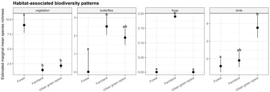
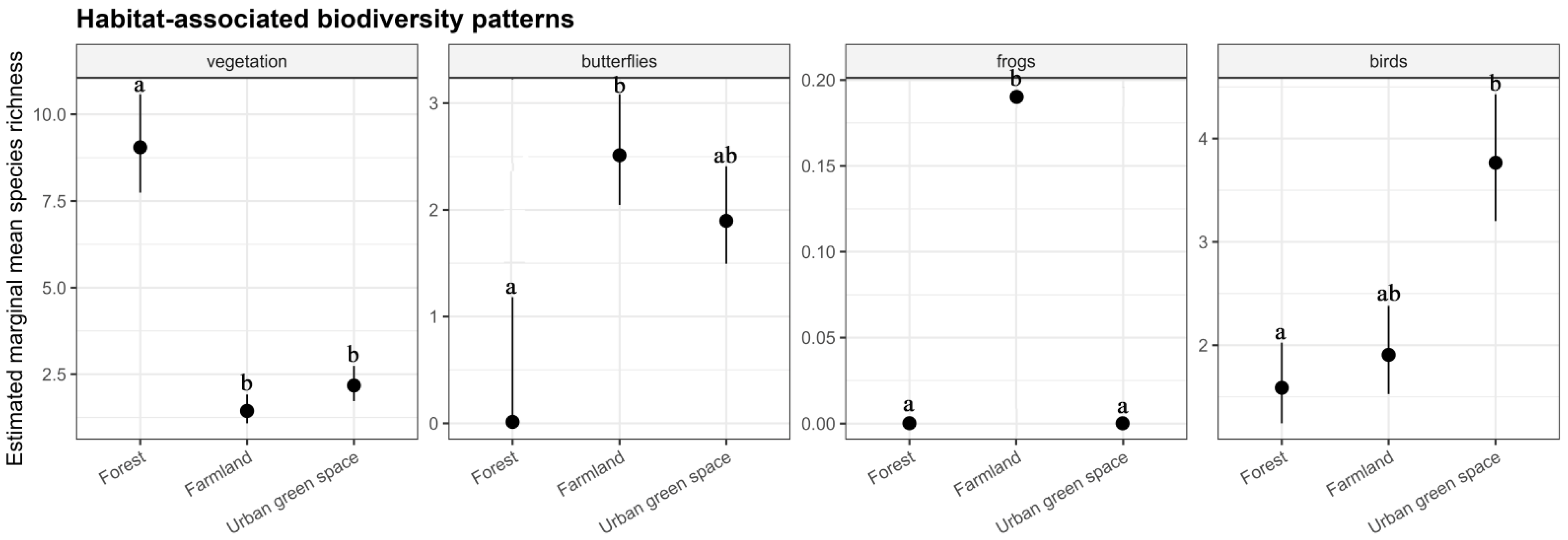
The habitat × season interaction was significant for the four taxonomic groups (or for the relevant response variables). Therefore, habitat effects are reported conditional on season. Figure 1 presents season-averaged marginal means for overview only; formal comparisons among habitats were performed within each season and are shown in Figure 2. The response patterns of different taxonomic groups to habitat type differed markedly, and no single habitat type maintained high species richness across all groups simultaneously. Vegetation showed a pattern closely aligned with natural habitats: species richness was highest in forest (~9.5), significantly higher than in farmland (~1.5) and urban green space (~2.5); the difference between farmland and urban green space was small. Butterflies displayed the opposite pattern: species richness in forest was close to zero, whereas richness in farmland (~2.5) and urban green space (~2.0) was markedly higher, with the two confidence intervals partially overlapping, indicating little difference between them. Frogs occurred almost exclusively in farmland (~0.19), with estimates close to zero in both forest and urban green space, indicating a strong dependence on farmland habitats. Birds exhibited the highest species richness in urban green space (~3.8), exceeding that in forest (~1.5) and farmland (~1.8); richness in forest and farmland was relatively similar, with overlapping confidence intervals (Figure 1).
Figure 1.
Estimated marginal mean species richness (with 95% confidence intervals) of four taxonomic groups (vegetation, butterflies, frogs, and birds) across three habitat types (forest, farmland, and urban green space). Note: Different lowercase letters above the points indicate statistically significant differences among habitat types within each taxonomic group based on estimated marginal means with Tukey adjustment (p < 0.05).
Figure 2.
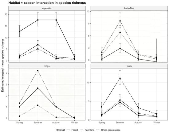
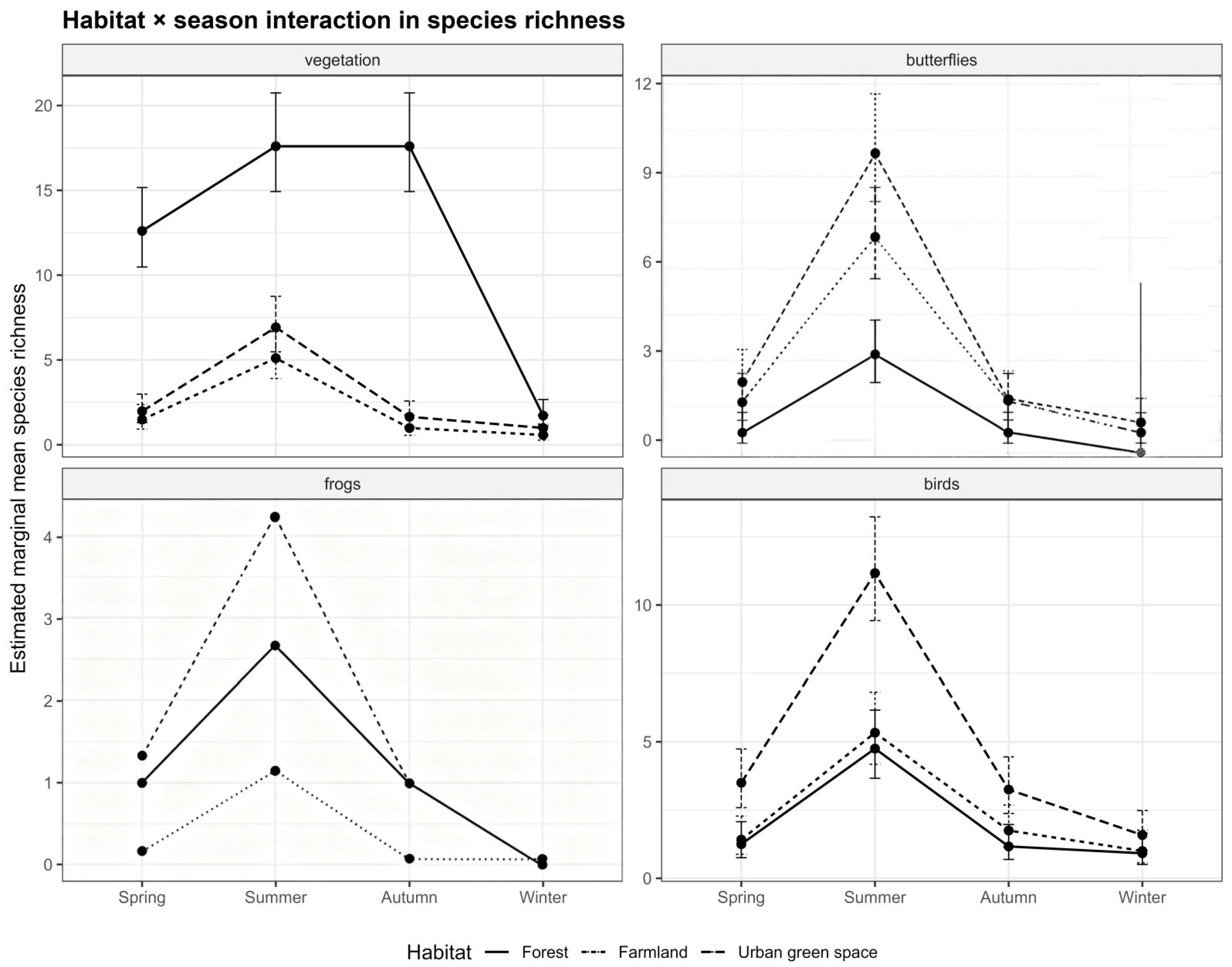
Estimated marginal mean species richness (with confidence intervals) of four taxonomic groups (vegetation, butterflies, frogs, and birds) across three habitat types (forest, farmland, and urban green space) and four seasons (spring, summer, autumn, and winter).
3.2. Within-Year Seasonal Variation and Habitat × Season Interactions
The effect of habitat on species richness is strongly season-dependent, i.e., there is a significant habitat × season interaction effect. All four taxa showed a consistent seasonal trend: species richness was highest in summer, lowest in winter, and intermediate in spring and autumn. Summer was not only the peak period of species richness for each taxon but also the period when differences among habitats were most pronounced; after winter arrived, species richness in the three habitats generally fell to low levels, and the differences narrowed markedly. Vegetation showed a pattern of absolute dominance by forest.
In forest, species richness in spring (approx. 12.5), summer (approx. 18), and autumn (approx. 18) was much higher than in farmland and urban green space. After peaking in summer and autumn, it dropped sharply to about 2.5 in winter. Farmland and urban green space showed smaller seasonal fluctuations, rising slightly in summer (to about 5 and 6.5, respectively), but in all seasons they were far lower than forest. The pattern for butterflies was opposite to that for vegetation. In summer, farmland had the highest species richness (approx. 10), followed by urban green space (approx. 7), and forest had the lowest (approx. 3.5); forest had the lowest butterfly richness in all seasons. In non-summer seasons, butterfly richness in all three habitats decreased markedly, and the differences among them narrowed accordingly. For frogs, detectable species records were found only in spring and summer; in autumn and winter, the estimated values for all three habitats were close to zero. The summer peak was highest in farmland (approx. 4.3), followed by forest (approx. 2.8), and lowest in urban green space (approx. 1.2); in spring, richness in all three habitats was relatively low, with little difference among them. Birds likewise showed the most prominent summer peak in urban green space (approx. 11.5), significantly higher than in farmland (approx. 5.5) and forest (approx. 4.5). In spring, autumn, and winter, bird richness in the three habitats was at relatively low levels, with small differences among habitats (Figure 2).
3.3. Cross-Taxon Statistical Covariation in Diversity Indices
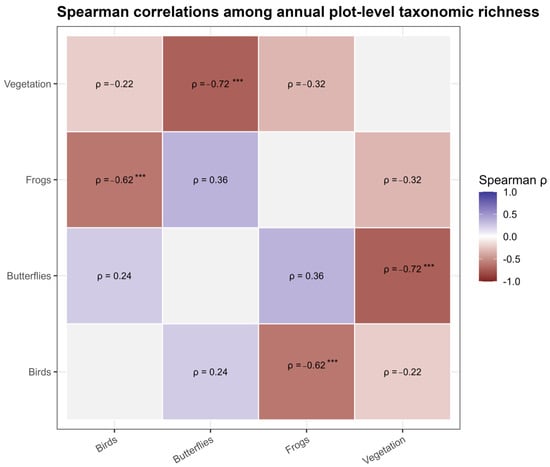
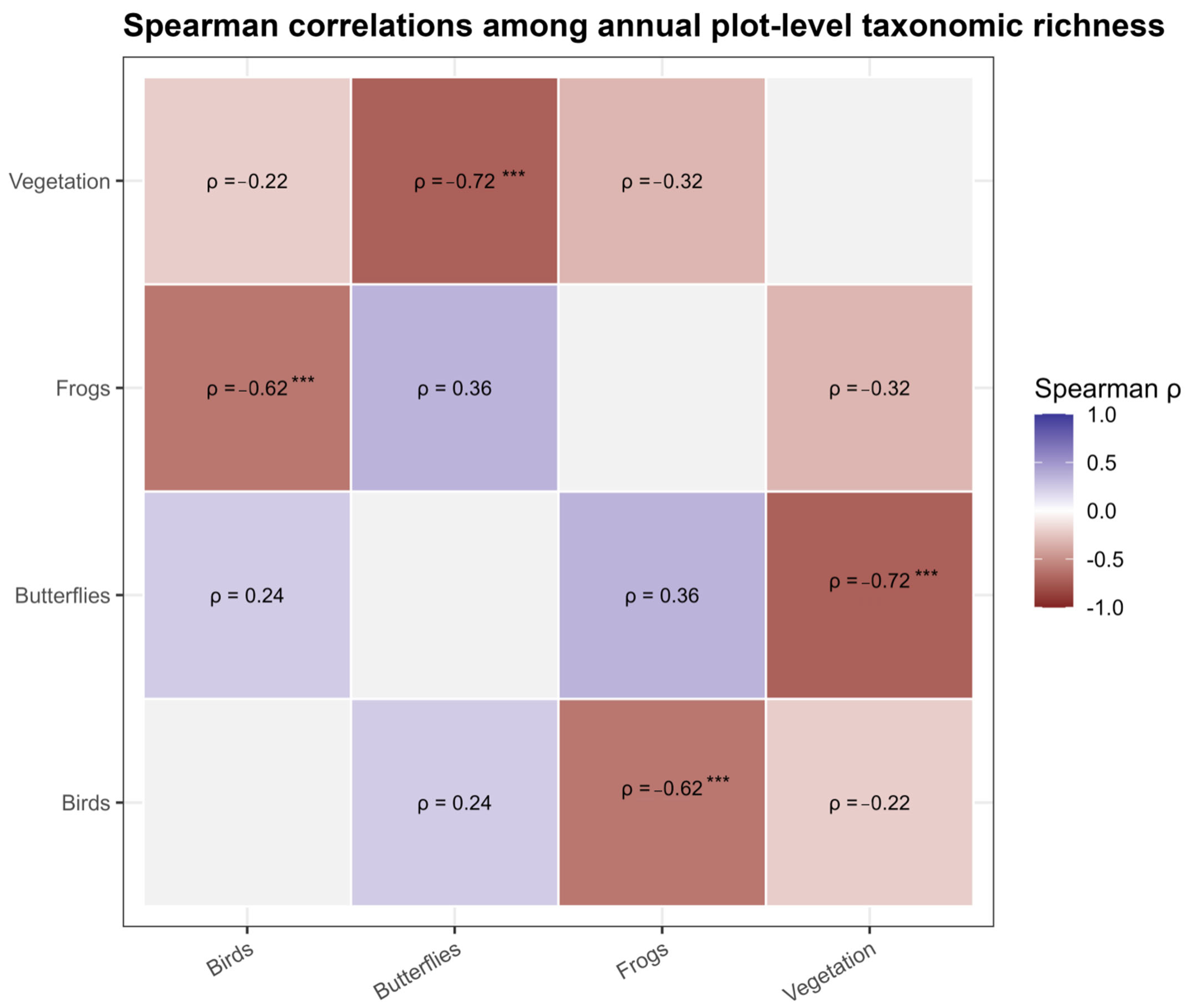
At the overall plot-scale level across all seasons in Dongyang, vegetation and butterflies exhibited a significantly strong negative correlation (Spearman ρ = −0.72, p < 0.001), i.e., plots with high vegetation richness harbored significantly lower butterfly richness, consistent with the habitat × season analysis. Frogs and birds also showed a significant strong negative correlation (ρ = −0.62, p < 0.001). All other pairwise relationships were weak: vegetation vs. frogs (ρ = −0.32) and vegetation vs. birds (ρ = −0.22) were weakly negative, while frogs vs. butterflies (ρ = 0.36) and butterflies vs. birds (ρ = 0.24) were weakly positive.
Habitat-specific analyses revealed a high degree of context dependency in inter-taxon relationships. In forests, vegetation and butterflies showed a strong positive correlation in the Shannon and Gini–Simpson indices (ρ = 0.70, p < 0.01), whereas vegetation and birds were significantly negatively correlated in the Shannon index (ρ = −0.53, p < 0.05) and Pielou’s evenness (ρ = −0.51, p < 0.05). In farmlands, vegetation and birds exhibited an extremely strong positive correlation, with all diversity indices reaching significance (Shannon ρ = 0.84, p < 0.05; Pielou ρ = 0.79; Gini–Simpson ρ = 0.80, p < 0.01); vegetation and butterfly abundance showed a moderate negative correlation (ρ = −0.54); frogs and butterflies were also moderately negatively correlated across diversity indices (ρ = −0.33 to −0.36). In urban green spaces, vegetation and butterflies showed near-perfect positive correlations (Shannon and Pielou ρ = 0.98; Gini–Simpson ρ = 0.95; abundance ρ = 0.67, p < 0.01); vegetation and frogs were moderately positively correlated (Shannon ρ = 0.51; Gini–Simpson ρ = 0.40); by contrast, birds showed trade-offs with other taxa and were negatively correlated with vegetation (ρ = −0.39) and butterflies (ρ = −0.37), and frogs and birds were also moderately negatively correlated in evenness (ρ = −0.39) and abundance (ρ = −0.40, Figure 3 and Figure S2).
Figure 3.
Habitat-specific Spearman rank correlations among species richness of vegetation, butterflies, frogs, and birds based on annual plot-level data. *** represents significance.
4. Discussion
4.1. Habitat-Associated Biodiversity Patterns Across Taxa
This study revealed clear habitat-associated differences in biodiversity, but the direction and magnitude of these differences were taxon-specific. No single habitat consistently supported the highest species richness across all four taxonomic groups. Vegetation richness was highest in forest, whereas butterflies showed higher richness in farmland and urban green space, frogs were most strongly represented in farmland, and birds exhibited the highest richness in urban green space. These contrasting patterns indicate that habitat-associated biodiversity responses cannot be adequately characterized by a single overall habitat ranking and instead depend on the ecological characteristics of individual taxonomic groups. The relatively high vegetation richness observed in forest is consistent with previous studies linking structurally complex habitats and greater environmental heterogeneity with higher plant diversity [35,36]. In contrast, farmland habitats supported relatively higher butterfly diversity and abundance, likely reflecting the availability of nectar resources and open habitat conditions associated with agricultural systems [15,37,38]. Urban green spaces generally exhibited lower diversity and higher dominance across multiple taxa, suggesting simplified community structures, consistent with global urban biodiversity decline patterns [39,40,41].
Importantly, these patterns should be interpreted as habitat-associated differences rather than effects of specific drivers, because environmental variables such as vegetation structure, management intensity, and microclimatic conditions were not directly quantified. Previous studies have shown that such factors can strongly influence biodiversity patterns [35,36], and they may co-vary with habitat categories. Therefore, the observed differences likely reflect combined effects of multiple environmental gradients embedded within habitat types, rather than a single underlying mechanism.
4.2. Within-Year Seasonal Variation and Habitat Dependence
Species richness showed pronounced within-year seasonal variation, but the magnitude and pattern of this variation differed among taxonomic groups and habitat types. Across the four taxonomic groups, richness generally increased toward summer and declined toward winter, although the magnitude of seasonal change varied among taxa. Vegetation showed particularly strong seasonal variation in forest, with richness increasing substantially during summer and autumn and declining sharply in winter. Butterflies and birds also showed pronounced summer peaks, whereas frog richness was concentrated mainly in spring and summer. These patterns are broadly consistent with seasonal changes in plant growth, resource availability, and animal activity in subtropical ecosystems [14,42,43]. The significant habitat × season interaction detected for the relevant responses indicates that seasonal variation cannot be interpreted independently of habitat context. In particular, differences among habitats were most apparent during periods of high biological activity, whereas habitat contrasts tended to become smaller during winter when richness declined across habitats. This pattern suggests that habitat-associated differences may be expressed most strongly during periods of elevated resource availability and biological activity. However, the strength and significance of this interaction should be considered separately for each taxonomic group rather than interpreted as a universal response across taxa.
Because the present study covers only one year, these results represent within-year seasonal variation during the monitoring period rather than long-term seasonal dynamics [21]. Interannual variation in temperature, precipitation, vegetation phenology, and resource availability may alter the magnitude or timing of seasonal peaks. Therefore, the observed seasonal trajectories should not be extrapolated to long-term temporal trends without multi-year observations [44,45]. The relatively weak seasonal differentiation observed in some urban green-space comparisons may be associated with more homogeneous environmental conditions or management regimes [17], but this interpretation remains tentative because microclimatic and management variables were not directly quantified. Overall, the seasonal results demonstrate that biodiversity assessments based on a single sampling period may capture only part of the variation occurring within a year. Repeated seasonal sampling is therefore important for distinguishing persistent habitat-associated differences from patterns that emerge only during particular periods of the annual cycle.
4.3. Limitations and Future Directions
Several limitations should be acknowledged. First, environmental variables were not explicitly measured, and habitat categories may therefore confound multiple factors, including elevation, vegetation structure, fragmentation, and management intensity. As a result, the study cannot isolate the relative importance of individual drivers, although previous research highlights the importance of microclimatic buffering and landscape complexity [35,36,37]. Second, the study is based on one year of sampling, which limits inference about long-term temporal patterns. Multi-year monitoring is needed to evaluate the consistency of observed within-year variation and to distinguish trends from stochastic variability [38]. Third, cross-taxon association methodological constraints such as taxon-specific sampling differences and the use of annual mean values may obscure peak ecological processes and resource pulses, potentially leading to conservative estimates of biodiversity responses. Addressing these limitations by incorporating quantitative environmental measurements, long-term datasets, and mechanistic modeling approaches would substantially improve our understanding of biodiversity responses to landscape transformation. Although previous studies have rarely evaluated cross-taxon associations simultaneously within the same landscape and across seasons, this study, by integrating vegetation, butterflies, frogs, and birds across forest, farmland, and urban green space in a subtropical landscape, not only demonstrates that biodiversity responses are taxon-specific and habitat-dependent and that the structure of cross-taxon covariation changes along anthropogenic gradients, but also, while emphasizing that these associations represent statistical relationships rather than causal interactions (and that the frog results are constrained by low detection probability, short seasonal activity, and zero-inflated counts, such that their near-zero estimates should not be interpreted as complete absence, thereby rendering the results potentially conservative), provides a more holistic perspective for biodiversity management in human-dominated landscapes and recommends that future studies employ occupancy models, multispecies models, or unified detection probability modeling for further validation.
5. Conclusions
This study demonstrates that biodiversity patterns across forest, farmland, and urban green space can be taxon-specific and season-dependent. No single habitat consistently supported the highest species richness across all four taxonomic groups. Forests supported the highest vegetation richness, whereas farmlands were particularly important for butterflies and frogs, and urban green spaces supported the highest bird richness. These contrasting responses indicate that habitat-associated biodiversity patterns cannot be adequately characterized using a single overall habitat ranking. Species richness also exhibited pronounced within-year seasonal variation. Across taxa, richness generally increased toward summer and declined toward winter, but the magnitude and timing of seasonal changes differed among taxonomic groups and habitats. The habitat × season interaction further indicated that habitat-associated differences were most apparent during periods of relatively high biological activity. Thus, biodiversity assessments based on a single sampling period may overlook important temporal variation. Cross-taxon associations were also highly context-dependent. Relationships among vegetation, butterflies, frogs, and birds differed in strength and, in some cases, direction among habitats. These patterns suggest that taxonomic groups do not respond independently to habitat conditions, but their associations vary according to the ecological context in which communities occur. However, because the present analyses were based on observational correlations, these relationships should not be interpreted as causal interactions.
Overall, our findings highlight the importance of integrating multiple taxonomic groups, multiple seasons, and habitat-specific analyses when assessing biodiversity in human-dominated landscapes. Forest, farmland, and urban green space each contributed differently to landscape-level biodiversity conservation. Effective biodiversity management should therefore move beyond a single-habitat or single-taxon perspective and adopt context-specific strategies that recognize complementary contributions of different habitat types. Long-term monitoring incorporating quantitative measurements of vegetation structure, microclimate, landscape configuration, and management intensity will be necessary to identify the mechanisms underlying the observed biodiversity patterns and cross-taxon associations.
Supplementary Materials
The following supporting information can be downloaded at: https://www.mdpi.com/article/10.3390/f17111303/s1, Figure S1: Sampling Site Distribution Map of Forest, Farmland and Urban Areas, Dongyang City; Figure S2: Spearman Correlation Matrix Heatmaps of Biodiversity Metrics and Abundance in Different Habitats.
Author Contributions
Conceptualization, L.Y. and H.X.; Methodology, L.Y. and L.G.; Software, C.W. (Chuping Wu); Validation, X.J. and H.X.; Formal Analysis, C.W. (Chuping Wu), J.J. and C.W. (Chaoran Wen); Investigation, L.Y. and L.G.; Resources, X.J. and H.X.; Data Curation, X.J.; Writing—Original Draft Preparation, L.Y.; Writing—Review & Editing, L.G.; Visualization, L.G.; Supervision, H.X.; Project Administration, H.X.; Funding Acquisition, L.Y. and L.G. All authors have read and agreed to the published version of the manuscript.
Funding
This research was financially supported by the Cooperation of Zhejiang Province and the Chinese Academy of Forestry (grant no. 2024SY10) and the “Pioneer” and “Leading Goose” R&D Program of Zhejiang (2024C03227).
Institutional Review Board Statement
Not applicable.
Informed Consent Statement
Not applicable.
Data Availability Statement
The data presented in this study are available in the article.
Acknowledgments
The authors thank everyone for their significant engagement in this project. We thank the editor and anonymous reviewers for their constructive comments to improve the manuscript. The datasets generated during the current study are available in the Supplementary Materials.
Conflicts of Interest
Liang Gao and Hong Xiao are employed by Zhejiang Environmental Monitoring Engineering; their employer’s company was not involved in this study, and there is no relevance between this research and their company. The remaining authors declare that the research was conducted in the absence of any commercial or financial relationships that could be construed as a potential conflict of interest. The funders had no role in the design of the study; in the collection, analyses, or interpretation of data; in the writing of the manuscript; or in the decision to publish the results.
References
- Simkin, R.D.; Seto, K.C.; McDonald, R.I.; Jetz, W. Biodiversity impacts and conservation implications of urban land expansion projected to 2050. Proc. Natl. Acad. Sci. USA 2022, 119, e2117297119, Correction in Proc. Natl. Acad. Sci. USA 2022, 119, e2208328119. [Google Scholar] [CrossRef] [Scilit]
- Chen, G.; Li, X.; Liu, X.; Chen, Y.; Liang, X.; Leng, J.; Xu, X.; Liao, W.; Qiu, Y.; Wu, Q.; et al. Global projections of future urban land expansion under shared socioeconomic pathways. Nat. Commun. 2020, 11, 537. [Google Scholar] [CrossRef] [Scilit]
- McDonald, R.I.; Beatley, T.; Elmqvist, T. The green soul of the concrete jungle: The urban century, the urban psychological penalty, and the role of nature. Sustain. Earth 2018, 1, 3. [Google Scholar] [CrossRef] [Scilit]
- Tiang, D.C.F.; Morris, A.; Bell, M.; Gibbins, C.N.; Azhar, B.; Lechner, A.M. Ecological connectivity in fragmented agricultural landscapes and the importance of scattered trees and small patches. Ecol. Process. 2021, 10, 20. [Google Scholar] [CrossRef] [Scilit]
- Campos, P.R.A.; Rosas, A.; de Oliveira, V.M.; Gomes, M.A.F. Effect of landscape structure on species diversity. PLoS ONE 2013, 8, e66495. [Google Scholar] [CrossRef] [Scilit]
- Hernandez, D.J.; David, A.S.; Menges, E.S.; Searcy, C.A.; Afkhami, M.E. Environmental stress destabilizes microbial networks. ISME J. 2021, 15, 1722–1734. [Google Scholar] [CrossRef] [Scilit]
- Finizio, M.; Pontieri, F.; Bottaro, C.; Di Febbraro, M.; Innangi, M.; Sona, G.; Carranza, M.L. Remote sensing for urban biodiversity: A review and meta-analysis. Remote Sens. 2024, 16, 4483. [Google Scholar] [CrossRef] [Scilit]
- Pereira, P.; Inácio, M.; Pinto, L.; Kalinauskas, M.; Bogdzevic, K.; Zhao, W. Mapping ecosystem services in urban and peri-urban areas: A systematic review. Geogr. Sustain. 2024, 5, 491–509. [Google Scholar] [CrossRef] [Scilit]
- Qiu, J.; Cardinale, B.J. Scaling up biodiversity-ecosystem function relationships across space and over time. Ecology 2020, 101, e03166. [Google Scholar] [CrossRef] [Scilit]
- Aronson, M.F.J.; Lepczyk, C.A.; Evans, K.L.; Goddard, M.A.; Lerman, S.B.; MacIvor, J.S.; Nilon, C.H.; Vargo, T. Biodiversity in the city: Key challenges for urban green space management. Front. Ecol. Environ. 2017, 15, 189–196. [Google Scholar] [CrossRef] [Scilit]
- Yan, Y.; Jarvie, S.; Zhang, Q.; Han, P.; Liu, Q.; Zhang, S.; Liu, P. Habitat heterogeneity determines species richness on small habitat islands in a fragmented landscape. J. Biogeogr. 2023, 50, 976–986. [Google Scholar] [CrossRef] [Scilit]
- Glišić, M.; Jakovljević, K.; Lakušić, D.; Šinžar-Sekulić, J.; Vukojičić, S.; Tabašević, M.; Jovanović, S. Influence of habitat types on diversity and species composition of urban flora-A case study in Serbia. Plants 2021, 10, 2572. [Google Scholar] [CrossRef] [Scilit]
- Pan, Y.; Birdsey, R.A.; Phillips, O.L.; Jackson, R.B. The structure, distribution, and biomass of the world’s forests. Annu. Rev. Ecol. Evol. Syst. 2013, 44, 593–622. [Google Scholar] [CrossRef] [Scilit]
- Zellweger, F.; De Frenne, P.; Lenoir, J.; Vangansbeke, P.; Verheyen, K.; Bernhardt-Römermann, M.; Baeten, L.; Hédl, R.; Berki, I.; Brunet, J.; et al. Forest microclimate dynamics drive plant responses to warming. Science 2020, 368, 772–775, Erratum in Science 2020, 368, eabd3881. [Google Scholar] [CrossRef] [Scilit]
- Priyadarshana, T.S.; Martin, E.A.; Sirami, C.; Woodcock, B.A.; Goodale, E.; Martínez-Núñez, C.; Lee, M.B.; Pagani-Núñez, E.; Raderschall, C.A.; Brotons, L.; et al. Crop and landscape heterogeneity increase biodiversity in agricultural landscapes: A global review and meta-analysis. Ecol. Lett. 2024, 27, e14412. [Google Scholar] [CrossRef] [Scilit]
- Tamburini, G.; Bommarco, R.; Wanger, T.C.; Kremen, C.; van der Heijden, M.G.A.; Liebman, M.; Hallin, S. Agricultural diversification promotes multiple ecosystem services without compromising yield. Sci. Adv. 2020, 6, eaba1715. [Google Scholar] [CrossRef] [Scilit]
- Sol, D.; Trisos, C.; Múrria, C.; Jeliazkov, A.; González-Lagos, C.; Pigot, A.L.; Ricotta, C.; Swan, C.M.; Tobias, J.A.; Pavoine, S. The worldwide impact of urbanisation on avian functional diversity. Ecol. Lett. 2020, 23, 962–972. [Google Scholar] [CrossRef] [Scilit]
- Thébault, E.; Fontaine, C. Stability of ecological communities and the architecture of mutualistic and trophic networks. Science 2010, 329, 853–856. [Google Scholar] [CrossRef] [Scilit]
- Tylianakis, J.M.; Laliberté, E.; Nielsen, A.; Bascompte, J. Conservation of species interaction networks. Biol. Conserv. 2010, 143, 2270–2279. [Google Scholar] [CrossRef] [Scilit]
- Lefcheck, J.S.; Byrnes, J.E.K.; Isbell, F.; Gamfeldt, L.; Griffin, J.N.; Eisenhauer, N.; Hensel, M.J.S.; Hector, A.; Cardinale, B.J.; Duffy, J.E. Biodiversity enhances ecosystem multifunctionality across trophic levels and habitats. Nat. Commun. 2015, 6, 6936. [Google Scholar] [CrossRef] [Scilit]
- Kharouba, H.M.; Ehrlén, J.; Gelman, A.; Bolmgren, K.; Allen, J.M.; Travers, S.E.; Wolkovich, E.M. Global shifts in the phenological synchrony of species interactions over recent decades. Proc. Natl. Acad. Sci. USA 2018, 115, 5211–5216. [Google Scholar] [CrossRef] [Scilit]
- Ehbrecht, M.; Seidel, D.; Annighöfer, P.; Kreft, H.; Köhler, M.; Zemp, D.C.; Puettmann, K.; Nilus, R.; Babweteera, F.; Willim, K.; et al. Global patterns and climatic controls of forest structural complexity. Nat. Commun. 2021, 12, 519. [Google Scholar] [CrossRef] [Scilit]
- Desaegher, J.; Chiron, F.; Bessa-Gomes, C. Nationwide study of the triple landscape gradient across natural, agricultural and urban areas for the richness of flower-visiting insects. Biol. Conserv. 2023, 288, 110355. [Google Scholar] [CrossRef] [Scilit]
- Zhao, J.; Yu, L.; Newbold, T.; Shen, X.; Liu, X.; Hua, F.; Kanniah, K.; Ma, K. Biodiversity responses to agricultural practices in cropland and natural habitats. Sci. Total Environ. 2024, 922, 171296. [Google Scholar] [CrossRef] [Scilit]
- R Core Team. R: A Language and Environment for Statistical Computing; R Foundation for Statistical Computing: Vienna, Austria, 2023. [Google Scholar]
- Bates, D.; Mächler, M.; Bolker, B.; Walker, S. Fitting Linear Mixed-Effects Models Using lme4. J. Stat. Softw. 2015, 67, 1–48. [Google Scholar]
- Brooks, M.E.; Kristensen, K.; Benthem, K.J.V.; Magnusson, A.; Bolker, B.M. Glmmtmb balances speed and flexibility among packages for zero-inflated generalized linear mixed modeling. R J. 2017, 9, 378–400. [Google Scholar] [CrossRef] [Scilit]
- Lenth, R.V. emmeans: Estimated Marginal Means, aka Least-Squares Means, R package version 1.10.1; R Foundation: Vienna, Austria, 2024.
- Hartig, F. DHARMa: Residual Diagnostics for Hierarchical (Multi-Level/Mixed) Regression Models, R package version 0.4.7; R Foundation: Vienna, Austria, 2024.
- Oksanen, J.; Blanchet, F.G.; Kindt, R.; Legendre, P.; Minchin, P.R.; O’Hara, R.B.; Simpson, G.L.; Solymos, P.; Stevens, M.H.H.; Wagner, H. vegan: Community Ecology Package, R package version 2.0-10; R Foundation: Vienna, Austria, 2013.
- Wickham, H. ggplot2: Elegant Graphics for Data Analysis; Springer: New York, NY, USA, 2016; ISBN 978-3-319-24277-4. [Google Scholar]
- Pebesma, E. Simple Features for R: Standardized Support for Spatial Vector Data. R J. 2018, 10, 439–446. [Google Scholar] [CrossRef] [Scilit]
- Lüdecke, D.; Ben-Shachar, M.S.; Patil, I.; Waggoner, P.; Makowski, D. Performance: An R Package for Assessment, Comparison and Testing of Statistical Models. J. Open Source Softw. 2021, 6, 3139. [Google Scholar] [CrossRef] [Scilit]
- Hothorn, T.; Bretz, F.; Westfall, P. Simultaneous Inference in General Parametric Models. Biom. J. 2008, 50, 346–363. [Google Scholar] [CrossRef] [Scilit]
- De Frenne, P.; Zellweger, F.; Rodríguez-Sánchez, F.; Scheffers, B.R.; Hylander, K.; Luoto, M.; Vellend, M.; Verheyen, K.; Lenoir, J. Global buffering of temperatures under forest canopies. Nat. Ecol. Evol. 2019, 3, 744–749. [Google Scholar] [CrossRef] [Scilit]
- LaRue, E.A.; Hardiman, B.S.; Elliott, J.M.; Fei, S. Structural diversity as a predictor of ecosystem function. Environ. Res. Lett. 2019, 14, 114011. [Google Scholar] [CrossRef] [Scilit]
- Sánchez, A.C.; Jones, S.K.; Purvis, A.; Estrada-Carmona, N.; De Palma, A. Landscape complexity and functional groups moderate the effect of diversified farming on biodiversity: A global meta-analysis. Agric. Ecosyst. Environ. 2022, 332, 107933. [Google Scholar] [CrossRef] [Scilit]
- Tscharntke, T.; Clough, Y.; Wanger, T.C.; Jackson, L.; Motzke, I.; Perfecto, I.; Vandermeer, J.; Whitbread, A. Global food security, biodiversity conservation and the future of agricultural intensification. Biol. Conserv. 2012, 151, 53–59. [Google Scholar] [CrossRef] [Scilit]
- O’Connor, M.I.; Gonzalez, A.; Byrnes, J.E.K.; Cardinale, B.J.; Duffy, J.E.; Gamfeldt, L.; Griffin, J.N.; Hooper, D.; Hungate, B.A.; Paquette, A.; et al. A general biodiversity–function relationship is mediated by trophic level. Nature 2017, 548, 111–114. [Google Scholar]
- Tournayre, O.; Littlefair, J.E.; Garrett, N.R.; Brown, A.S.; Allerton, J.J.; Cristescu, M.E.; Clare, E.L. Contrasted effects of human pressure on biodiversity in the UK: A multi-taxonomic assessment using airborne environmental DNA. Ecography 2025, 2025, e08196. [Google Scholar] [CrossRef] [Scilit]
- Aznarez, C.; Svenning, J.C.; Pacheco, J.P.; Have Kallesøe, F.; Baró, F.; Pascual, U. Luxury and legacy effects on urban biodiversity, vegetation cover and ecosystem services. npj Urban Sustain. 2023, 3, 47. [Google Scholar] [CrossRef] [Scilit]
- Hillebrand, H.; Blasius, B.; Borer, E.T.; Chase, J.M.; Downing, J.A.; Eriksson, B.K.; Filstrup, C.T.; Harpole, W.S.; Hodapp, D.; Larsen, S.; et al. Biodiversity change is uncoupled from species richness trends: Consequences for conservation and monitoring. J. Appl. Ecol. 2018, 55, 169–184. [Google Scholar] [CrossRef] [Scilit]
- Yang, L.H.; Rudolf, V.H.W. Phenology, ontogeny and the effects of climate change on the timing of species interactions. Ecol. Lett. 2010, 13, 1–10. [Google Scholar] [CrossRef] [Scilit]
- Van Der Plas, F. Biodiversity and ecosystem functioning in naturally assembled communities. Biol. Rev. 2019, 94, 1220–1245. [Google Scholar] [CrossRef] [Scilit]
- Gu, Q.; Yu, Q.; Grogan, P. Cryptogam plant community stability: Warming weakens influences of species richness but enhances effects of evenness. Ecology 2023, 104, e3842. [Google Scholar] [CrossRef] [Scilit]
Disclaimer/Publisher’s Note: The statements, opinions and data contained in all publications are solely those of the individual author(s) and contributor(s) and not of MDPI and/or the editor(s). MDPI and/or the editor(s) disclaim responsibility for any injury to people or property resulting from any ideas, methods, instructions or products referred to in the content. |
© 2026 by the authors. Licensee MDPI, Basel, Switzerland. This article is an open access article distributed under the terms and conditions of the Creative Commons Attribution (CC BY) license.