


Abstract
Forest type maps require periodic revision, yet field inspection of every stand is impractical. This study tested whether stand-level disagreement between a Sentinel-2 U-Net classifier and the Republic of Korea’s forest type map could support screening for revision. A seven-class U-Net was trained using seasonal Sentinel-2 composites from 2025, and pixel predictions were aggregated to forest stands. Disagreeing stands passing dominance and confidence thresholds were flagged and assessed by blinded interpreters using high-resolution basemaps supplemented by Sentinel-2 composites. Stand-level agreement with the map was 0.69 by stand count and 0.76 when area-weighted. In the primary analysis, high-precision-class flags were mismatched in 41.3% of interpreted stands (29.7% when population-weighted), compared with 7.7% of controls. Test-set class precision, the pre-specified prioritization criterion, did not distinguish more reliable flags in this analysis. An exploratory partition by flag type yielded weighted rates of corresponding mismatches of 80.9% for stocking-status flags and 26.0% for species-dominance flags, representing 12.3- and 2.4-fold enrichment over their respective region-wide baselines. Approximately 35% of flagged stands were estimated to be mismatches, and the flags captured approximately 7.5% of estimated mismatches. These findings support model–map disagreement as a potential tool for prioritizing stand verification in the study region.
1. Introduction
The national forest type map (FTM) is a fundamental input for forest management and carbon stock accounting [1]. In the Republic of Korea, the FTM is constructed by interpreting large-scale aerial photographs together with field surveys. The map is revised zone by zone: the country is divided into five zones and one zone is updated each year, so any given zone is revised only once every five years [1]. A map can differ from the actual ground conditions for two reasons. First, differences in spatial resolution and stand delineation criteria may cause the existing forest type map and satellite-derived classifications to represent forest heterogeneity differently, leading to discrepancies between them; second, the forest may have changed since the map was produced. The update cycle makes the second reason unavoidable because even a perfectly interpreted map can be up to five years out of date for a given zone. These discrepancies may involve the species dominating a stand or the presence of tree cover, both of which the FTM scheme can represent because it includes a non-stocked forest class alongside its species classes. As field inspection of every stand is impractical, remote sensing has become a cost-effective means of monitoring forest conditions and identifying stands that require closer inspection [2,3,4,5].
Satellite classification of forest types is well suited for this task. The Sentinel-2 time series has been widely adopted because the imagery is freely available, and its high revisit frequency captures the seasonal spectral variation that can help distinguish species [6,7]. However, classification performance varies across settings and class schemes, and reliable species separation over large heterogeneous forests remains difficult [8,9,10]. Recent benchmarks for national-scale forests in the Republic of Korea reported F1 values near 0.55 using Sentinel-2 data alone [11], and performance remains low in the fragmented, species-rich forests of the Seoul–Gyeonggi metropolitan area, where a study of nine dominant species achieved a maximum overall accuracy of only 61% with a U-Net approach [12]. There is also a mismatch between the spatial units. Forest-type classifiers usually make predictions at the pixel level, whereas the FTM is defined and managed at the stand level, which is the unit to which a management prescription such as thinning or harvesting is applied [13,14].
Existing forest maps commonly supply labels for training and evaluating satellite classifiers. In these studies, map errors are primarily considered in terms of their effects on classifier training and evaluation. Discrepancies between outdated training labels and current imagery can be treated as label noise [15], addressed by tolerating or downweighting potentially mislabeled samples [16], or screened to identify labels for removal [17,18] or human review [19]. Bi-temporal change detection instead compares imagery from different dates to identify changes on the ground [20,21,22]. Such comparisons do not directly test whether a current image agrees with the existing map; an unchanged stand that was mislabeled during map production may therefore remain undetected. Image-to-map discrepancy detection directly addresses consistency between imagery and an existing map. Radoux and Defourny [23], for example, compared a topographic vector database with a QuickBird image using iterative trimming and evaluated discrepancies including clear cuts, regeneration, and incorrect forest types. Building on these precedents, the present study addresses a specific question for FTM revision: whether disagreement between a classifier trained on map-derived labels and the same map can identify existing stands with a higher likelihood of image–map mismatch. Answering this question requires evaluation of the screening output beyond classifier agreement with the map.
To address this question, we evaluate model–map disagreement as a signal for prioritizing stand verification for FTM updating. A standard U-Net is trained using FTM-derived labels and multi-season Sentinel-2 imagery from a single target year. Its pixel predictions are aggregated to FTM stand polygons, the units used for map revision. The screening targets potential discrepancies arising from original mapping errors or post-mapping changes; the present design cannot distinguish these sources. The study quantifies screening yield and enrichment relative to a regional baseline through blinded interpretation of flagged, control, and ungated stands and population weighting.
Three considerations motivate this approach. First, a model trained on map labels need not reproduce every label: in the presence of label noise, deep-learning models can learn generalizable patterns before memorizing mislabeled examples [24,25]. Second, screening is useful when image–map mismatches are concentrated among a manageable set of flags. Agreement with the FTM alone cannot establish this, because the map supplies both the training labels and the classifier’s evaluation reference. A model prediction that correctly departs from an erroneous map label would be scored as an error against that reference. We therefore assess the screening output through interpretation of high-resolution imagery, with interpreters blinded to model predictions and group assignments. This provides evidence beyond agreement with the FTM, but does not eliminate dependence: the model may reproduce map errors, and supplementary use of the Sentinel-2 inputs may introduce correlated errors into the interpretation. Third, aggregating predictions to FTM polygons places the model–map comparison on the units that would be inspected and updated.
As the number of flagged stands may exceed the capacity for independent review, the flags also require a basis for prioritization. We therefore examine test-set class precision as a potential criterion, on the reasoning that classes with higher map-based precision might yield more reliable disagreement flags. We address two questions: (1) are model–map disagreement flags enriched for image–map mismatches, and if so, what proportion of the flags are mismatched, and (2) can test-set class precision serve as a useful criterion for prioritizing the resulting flags? We additionally explore whether flag validity varies with the type of disagreement, particularly whether non-stocked forest is involved in the mismatch.
2. Materials and Methods
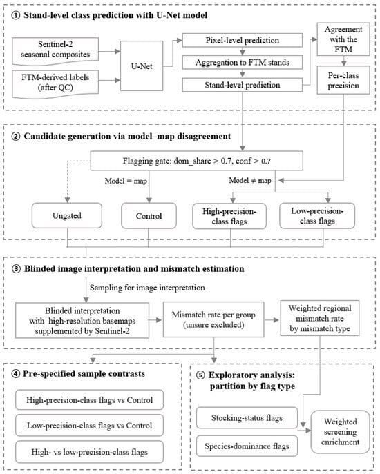
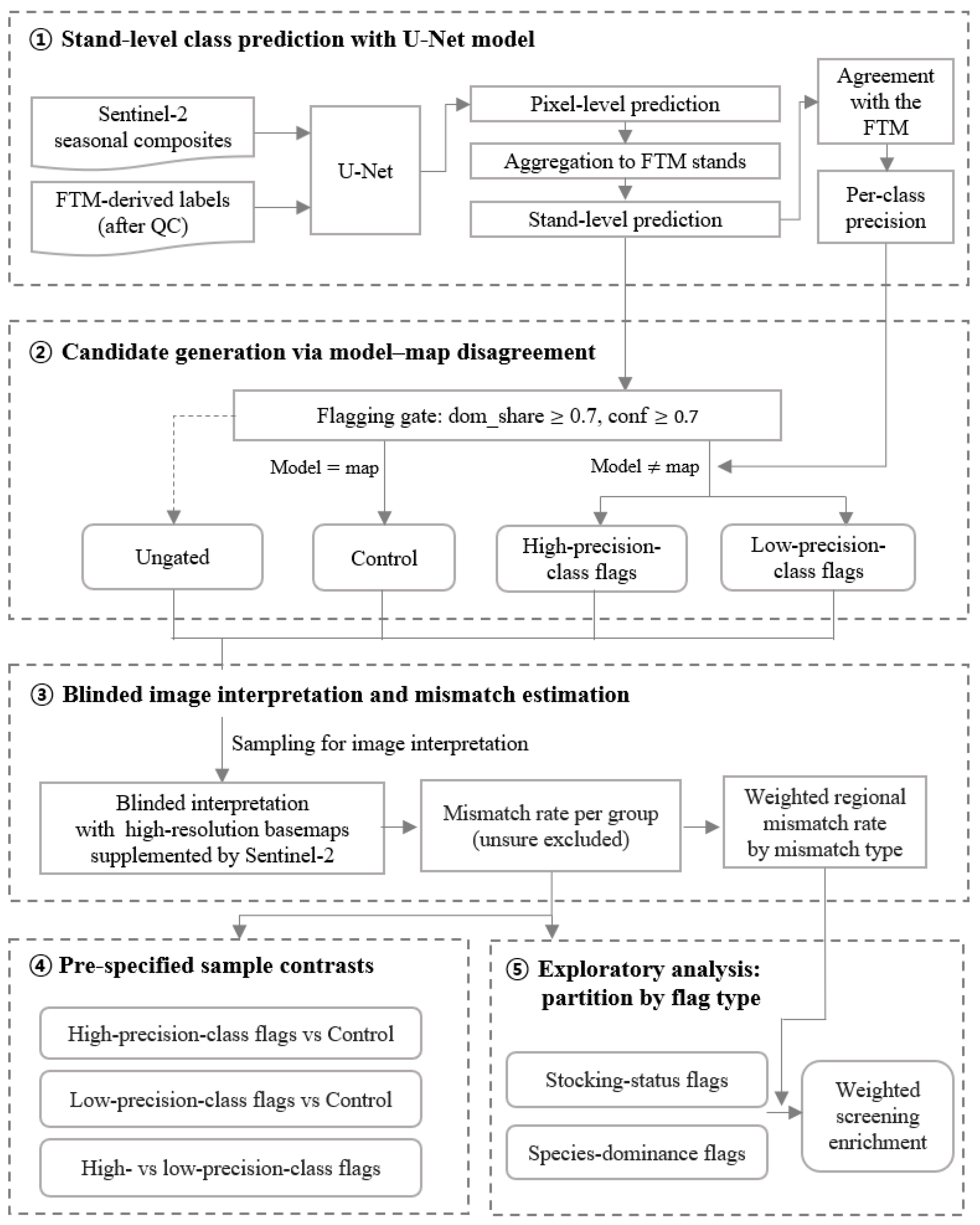
The method consisted of five steps (Figure 1). First, FTM labels and Sentinel-2 seasonal composites were prepared, a U-Net was trained, and its predictions were aggregated to FTM stand polygons for agreement assessment (Section 2.1 and Section 2.2). Second, disagreeing stands passing dominance and confidence gates were flagged and stratified by the test-set precision of the model-predicted class (Section 2.3). Third, high- and low-precision-class flags, controls with model–map agreement, and ungated stands were sampled for blinded image interpretation (Section 2.4). Fourth, sample-based contrasts tested whether flags were enriched for image–map mismatches and whether class precision could prioritize them (Section 2.4.3 and Section 3.2.2). Fifth, exploratory analyses partitioned flags by disagreement type, and weighted estimates described the flagged population and the region-wide mismatch baseline (Section 2.4.3 and Section 3.2.4).
Figure 1.
Research framework. FTM, forest type map; dom_share, proportion of a stand’s pixels carrying the model-dominant class; conf, mean pixel confidence across the stand. Solid arrows indicate the flow of data and analyses, while the dashed arrow indicates stands that do not pass the flagging gate.
2.1. Study Area and Class Scheme
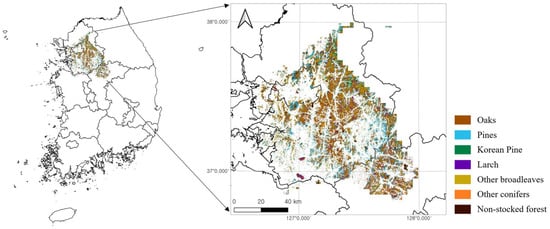
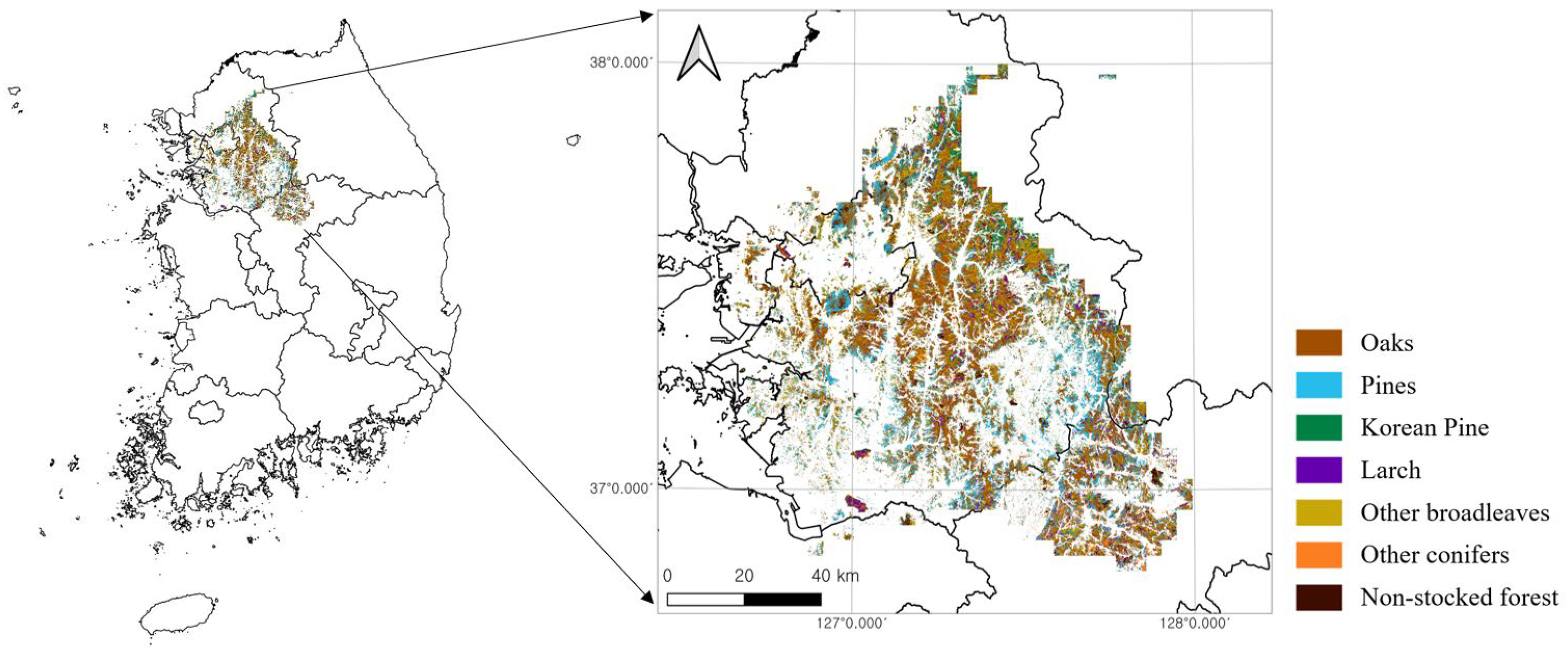
This study was conducted in the Seoul–Gyeonggi region of the central Republic of Korea (approximately 37° N, 127° E), corresponding to one of the eight forest regions delineated by Lee et al. (2025) [12] through k-means clustering of standardized kernel-density maps for 43 forest tree species (Figure 2). The region comprises roughly 361,981 ha of temperate forest across terrain ranging from 3.2 to 906.4 m in elevation, encompassing both coniferous and deciduous stands characteristic of the central Korean Peninsula. While the previous study targeted nine single-species-dominated stands [12], the present analysis addressed stand-level, polygon-based classification under a scheme of seven forest-type classes consolidated from the classification categories of the FTM. Specifically, Pinus densiflora, P. rigida, and P. thunbergii were merged into the pine class, and Robinia pseudoacacia was placed into the other broadleaves class. These species were merged because they are difficult to separate reliably at the 10 m resolution of Sentinel-2 and several were represented by too few stands to train separate classes. The consolidation reduces the thematic resolution of the screening, as disagreements among the merged species cannot be detected. Among these, “other broadleaves” and “other conifers” are catch-all classes intended to comprehensively cover minor species occupying small areas; therefore, each contains several forest types. Coniferous–broadleaf mixed forests, in which multiple species are intermingled so that no single dominant species is defined, cannot be included as targets of the model–map dominance comparison; accordingly, those polygons were excluded from the analysis (35,422 stands covering 44,384 ha, or 12.3% of the forest area). The number and area of stands in each class are given in Table 1.
Figure 2.
Study area in Seoul–Gyeonggi region of the Republic of Korea, corresponding to the spatial extent used by Lee et al. (2025) [12]. Colors indicate the seven stand classes consolidated from the FTM (Table 1).
Table 1.
Consolidated seven-class scheme. Numbers and areas refer to FTM stands within the study region (235,788 stands, 317,597 ha in total); the test-stand counts refer to the common test set used in all three replicates (Section 2.2.3).
2.2. Forest-Type Classification
2.2.1. Sentinel-2 Inputs, Reference Labels, and Data Splits
The inputs were derived from the 2025 Sentinel-2 Surface Reflectance Harmonized product and composited in Google Earth Engine [26]. Three seasonal median composites were used to exploit phenological differences among broadleaf, coniferous, and larch species: April for leaf-out, September for peak canopy, and November for pre-abscission. For each season, 10 spectral bands, seven vegetation indices, and seven GLCM texture features were combined into 24 channels, with the three seasonal composites concatenated and four time-invariant topographic channels (elevation, slope, and the sine and cosine of aspect) appended, yielding a 76-channel input at 10 m resolution over a 4 × 4 km fishnet grid. The 20 m bands were resampled to the 10 m grid by bilinear interpolation in Google Earth Engine; this does not increase their effective spatial resolution, and the texture features were derived only from the native 10 m near-infrared band (B8; Table S2). Full details of the compositing procedure, cloud masking, vegetation indices, GLCM definitions, and topographic channel processing are provided in Supplementary Material S1 (Sections S1.1–S1.4; Tables S1 and S2). The number of valid (unmasked) observations contributing to each composite was recorded per pixel; across stands in the study region, its median was 7 for April, 2 for September, and 5 for November, with small differences among classes (Appendix F).
The training labels were derived from a 2025 1:5000 FGIS forest type map [27]. The 2025 date refers to the database release. Because the FTM is revised zone by zone on a five-year cycle, the interpretation underlying a stand may predate the release; in the study region, the most recent revision cycle before the 2025 release covered the area in 2023 (second cycle, 2020–2024) [1], although partial updates have been incorporated into subsequent releases. Protected areas and infrastructure-related features (airports, military sites, power plants, industrial and port land, waterworks, and areas near access routes) retrieved from OpenStreetMap with OSMnx on 15 May 2026 [28,29] were masked. Mixed coniferous–broadleaf stands and stands containing fewer than 50 pixels on the 10 m grid (0.5 ha) were removed. The latter cutoff retains a nominal footprint of 50 grid pixels, equivalent in area to approximately 12.5 native 20 m pixels, and reduces the influence of very small polygons in stand-level aggregation. It also corresponds to the minimum area in the FAO forest definition [30]. The stands remaining after these steps are termed evaluable, and population quantities below refer to this set. Before assignment to data splits, candidate 4 × 4 km cells were excluded if visual inspection indicated that 10% or more of their area had changed since mapping or was affected by residual haze or clouds. Stands in excluded cells remained evaluable and eligible for region-wide prediction, flagging, and image-based assessment but were not used for training, validation, or test-set agreement assessment. Label preparation is detailed in Supplementary Material S1 (Section S1.5).
Model-fitting and evaluation sets were drawn from the retained candidate cells. Splits were assigned at the level of spatial blocks rather than individual stands. These 4 × 4 km fishnet cells served as spatial blocks, and each cell was assigned to one of the training, validation, or test sets. As forest area and class composition vary spatially, cells were scored for rarity. The score of a cell was defined as the sum, over classes, of its pixel count for a class divided by that class’s total pixel count in the region, so that cells containing scarce classes were prioritized. To allow the replicates to reflect variability arising from the spatial selection of training cells, and not only from model initialization, a seed-dependent multiplicative perturbation of up to ±20% was applied to these scores. This value was set heuristically so that cells with similar scores could exchange positions between replicates, while cells containing scarce classes retained their priority. Cells were then considered in that order and assigned to a split until the accumulated pixel count of every class in every split lay within ±10% of that class’s target for the respective split, with targets of 24% of each class’s pixels for training and 3% each for validation and test; the tolerance was relative to the target count. In total, 79 cells were selected. As the selection process terminates only once the rarest class meets its quota in every split, the number of cells assigned to each split was determined by that class rather than being fixed in advance; 55 of the 79 cells were assigned to training, 10 to validation, and 14 to testing. The test cells were held fixed across all three replicates. Table S3 in Supplementary Material S1 reports the allocation used for the first replicate and subsequent analyses.
2.2.2. Model Architecture and Training
Species prediction was performed using a standard U-Net semantic-segmentation network [31] with a 76-channel input and seven active classes, as shown in Table 1. The model was trained three times under the same configuration with different random seeds, varying model initialization and the spatial selection of training cells while keeping the test cells fixed (Section 2.2.1). Agreement with the FTM is reported as the mean ± SD across the three replicates. The first replicate was used for the region-wide prediction, from which flags were derived.
To assess the contribution of each predictor group, the model was additionally trained with four nested predictor sets: spectral bands only (30 channels), bands and vegetation indices (51), bands, indices, and GLCM texture (72), and all 76 variables. Each set was trained three times with different random seeds for model initialization, while the allocation of cells to splits (Table S3) was held fixed, and evaluated on the same test stands (Appendix D). The network architecture, input-tensor construction, and full training configuration are reported in Supplementary Material S1 (Sections S1.6–S1.8; Table S4).
The trained model was then applied to each cell within the study region. Within each cell, 256 × 256 pixels were extracted at a stride of 128 pixels, with the final tile of each row and column aligned to the cell edge such that no pixels were left uncovered. Class probabilities from overlapping tiles were averaged before the argmax operation, providing a soft vote rather than a majority vote over hard labels. Three rasters were generated per cell: predicted class, pixel confidence, and pixel decision margin. Further details are provided in Supplementary Material S1 (Section S1.9).
2.2.3. Stand-Level Aggregation and Agreement Assessment
The stand was adopted as the unit at which model output is read. Aggregation used the polygons of the forest type map itself, rather than a new segmentation of the imagery, so that the comparison fell on the very units that would be inspected and updated. For each polygon, the model-dominant class was defined as the class represented by the largest number of pixels, and its areal share among those pixels was denoted as dom_share. The mean pixel confidence over all pixels within the stand was denoted as conf.
Agreement with the FTM was assessed at the stand level using test cells withheld from training. The same 5797 test stands were used in all three replicate runs described in Section 2.2.2, and their class composition is reported in Table 1 and Table 2. We reported overall agreement, defined as the proportion of test stands whose model-dominant class matched the map-dominant class, by stand count and area weighting (the total pixel count of agreeing stands divided by that of all test stands), together with macro- and weighted-F1, per-class precision/recall/F1, and confusion matrices. These measures describe agreement with the FTM, which is itself the audit target, rather than accuracy against an independent vegetation reference. Mean per-class precision across the three replicates was used for class-precision stratification.
Table 2.
Per-class agreement with the FTM, stand units (mean ± SD, 3 replicates). Low-precision classes (precision < 0.60) shaded. N denotes the number of test stands in each map class; the same test stands were used in all three replicates.
2.3. Flagging Framework
2.3.1. Flag Definition and Thresholds
A stand whose model-dominant class differed from its map-dominant class was termed a disagreeing stand. Disagreeing stands satisfying dom_share ≥ 0.70 and conf ≥ 0.70 were termed flagged stands, or flags. Here, dom_share is the proportion of pixels within a stand assigned to the model-dominant class, and its cutoff of 0.70 was used as an operational screening criterion. The confidence cutoff of 0.70 was selected before image interpretation. Sensitivity to the confidence cutoff was evaluated over 0.60–0.80 while holding dom_share ≥ 0.70 fixed (Appendix B, Table A1).
2.3.2. Class-Precision Stratification
Test-set class precision was evaluated as a potential criterion for prioritizing disagreement flags. Precision was defined as the proportion of stands predicted as a given class for which the map label was the same class, and a threshold of 0.60 was used for stratification. Flags were then assigned to the high- or low-precision stratum according to the precision of the class predicted by the model and were termed high-precision-class flags and low-precision-class flags, respectively. High-precision-class flags were used in the primary contrast, whereas low-precision class flags were analyzed separately to assess the utility of the precision criterion. As no established convention exists for this bound, the value 0.60 was therefore set a priori and its influence was assessed by recomputing the contrast at 0.55 and 0.65 (Appendix C, Table A2).
2.4. Image-Based Evaluation Design
2.4.1. Sampling Design
Four groups of stands were sampled for interpretation: high-precision-class flags, low-precision-class flags, a control group, and an ungated group. The control group consisted of stands meeting the same gate criteria, but for which model dominance was equal to map dominance, drawn from high-precision classes only. Per-group sample sizes were set to estimate each group’s mismatch rate at 95% confidence with an allowable sampling error of ±10 percentage points under worst-case variance, yielding approximately 95 stands per group [32] (z = 1.96, p = 0.5, d = 0.10, with finite-population correction). The primary analysis used stands in the high-confidence interval (conf ≥ 0.70); stands sampled from the relaxed interval (0.60 ≤ conf < 0.70) were used only for the threshold-sensitivity analysis. Of the 405 gated stands interpreted, 265 fell into the high-confidence interval (94 high-precision-class flags, 79 controls, and 92 low-precision-class flags) and 140 fell into the relaxed interval (48, 44, and 48, respectively). The precision of each estimated mismatch rate was reported as a Wilson’s 95% confidence interval [33].
The interpretation sample targeted screening within the region used for model training and application. Stands were sampled randomly across this regional population, including cells used for training. As stand polygons can straddle 4 × 4 km cell boundaries, a stand may fall partly inside a training cell and partly inside a validation or test cell. Each stand was therefore assigned to the split that covered the largest proportion of its area, so that every stand carried a single provenance label. Stands lying outside all 79 selected cells were labelled as belonging to the no-split group. Split provenance was reported alongside the primary results, because disagreement in a stand whose FTM label was included in the training data provides a direct test of whether the model reproduced the map.
Flag sampling was stratified by confusion pair (map dominance → model dominance), with caps on individual pairs to prevent common pairs from dominating the sample. Inclusion probabilities were therefore non-uniform, and population estimates used weighting (Section 2.4.3). Control quotas were based on the map-class proportions in the high-precision-class flag sample, and agreeing stands were randomly selected within the represented high-precision classes. No controls were drawn from non-stocked forest or other conifers, so quotas for flags with either of these map classes could not be filled. Controls were therefore only partially matched to flag composition, and the control group was smaller than its target size.
The ungated group was sampled to characterize the regional base rate of mismatches among stands outside the flagging gate. This group consisted exclusively of stands that failed the flagging criteria (dom_share < 0.70 or conf < 0.70), regardless of whether the model and map dominance agreed. A total of 96 stands were selected by simple random sampling from this ungated stratum and interpreted using the protocol described in Section 2.4.2. The sample size was determined using the same rule as for the other groups [32] (z = 1.96, p = 0.5, d = 0.10, with finite-population correction). The overall mismatch rate was estimated by combining the group-specific mismatch rates using the corresponding stratum sizes as weights.
2.4.2. Blinded Image Interpretation
The sampled stands were reviewed independently by three interpreters with expertise in forest remote sensing, who were blinded to the model prediction and group assignment. Dominant forest-type classes were assessed primarily from high-resolution basemaps available in QGIS (Google Satellite, Esri Satellite, and VWorld), using visible crown form, texture, and color. The 2025 Sentinel-2 composites were inspected as supplementary evidence of possible harvesting, clearing, development, or other land-cover differences discernible at 10 m resolution. These composites were not used to determine the dominant species.
For each stand, interpreters assessed whether the mapped class agreed with the class identified in the available imagery. Each interpreter assigned a verdict of match, mismatch, or unsure. Mismatches were assigned a type: species-dominance, where both sources indicated stocked forest but differed in dominant class, or stocking-status, where they differed in the presence of established tree cover. The latter included open or recently cleared land, early regeneration, conversion to built land, and tree cover on land mapped as non-stocked. Final verdicts were determined by majority vote; stands with three different verdicts were resolved by consensus adjudication after the independent interpretations. An image–map mismatch denotes a difference between the interpreted forest-type class and the FTM label. A model–map disagreement denotes a difference between model and map classes (Section 2.3.1).
2.4.3. Statistical Analysis
Mismatch rates were calculated among resolved stands (match + mismatch); final unsure verdicts were excluded from the denominator and reported separately. The primary analysis used conf ≥ 0.70. High-precision-class flags were compared with controls, low-precision-class flags with controls, and the two precision strata with each other. Two-sided Fisher’s exact tests were used for these sample-based contrasts because several counts were small, and Wilson 95% confidence intervals were calculated for sample proportions. These unweighted comparisons describe the selected sample composition, not population-weighted effects, and treat stands as independent observations. To assess interpreter variability, group mismatch rates and the high-precision-class–control contrast were also calculated separately from each interpreter’s independent verdicts (Appendix E). Inter-interpreter agreement was summarized by Fleiss’ κ [34] and the proportions of three-way and pairwise agreement.
Population-level quantities were weighted to account for the unequal sampling allocation. Species-dominance flag rates were weighted by confusion-pair population sizes. Stocking-status flag rates used three weighting groups: mapped stocked but predicted non-stocked (N = 403), mapped non-stocked but predicted as a high-precision class (N = 131), and mapped non-stocked but predicted as other conifers (N = 69). Within each weighting group, the mismatch proportion among resolved interpretations was applied to the corresponding population size.
Region-wide rates combined flagged, agreeing gated, and ungated stands in proportion to their population sizes (4303, 29,576, and 82,830). Estimates were obtained overall and by interpreted mismatch type. The agreeing gated population is termed the control stratum below, although its sample included high-precision classes only. Because controls were sampled to approximate flag composition, their rates were post-stratified by map-dominant class. The 1600 agreeing stands in low-precision classes were assigned the post-stratified control rate; alternatives of 0% and 25% were examined. Weighted confidence intervals were calculated using a stratified normal approximation.
Analyses not specified in advance were treated as exploratory. For exploratory analyses, flags were partitioned by flag type based on the map–model class pair. Flags in which non-stocked forests appeared on either side were termed stocking-status flags. The remainder, in which both sources indicated stocked forests but disagreed on the dominant species, were termed species-dominance flags. These flag types were defined from the map–model class pair alone, not from the mismatch type recorded during image interpretation. The contrasts between flag types were tested on the unweighted interpreted sample using the procedures described above. The ungated stratum was likewise divided into stands for which model and map dominance agreed and those for which they disagreed. Screening enrichment was defined as the weighted rate of corresponding mismatches among the stands of a given flag type, divided by the region-wide rate of the same mismatch type. For species-dominance flags, the corresponding mismatches were species-dominance mismatches; for stocking-status flags, they were stocking-status mismatches.
3. Results
3.1. Model Performance
In the stand-level evaluation, overall agreement with the FTM was 0.69 ± 0.03 by stand count and 0.76 ± 0.03 when area-weighted, with macro-F1 of 0.67 ± 0.04 and weighted-F1 of 0.68 ± 0.04 (mean ± SD, N = 3). Precision was high for pines (0.88 ± 0.01), larch (0.78 ± 0.05), and other broadleaves (0.78 ± 0.04); Korean pine (0.66 ± 0.02) and oaks (0.63 ± 0.05) also met the precision criterion, resulting in five of the seven classes being assigned to the high-precision stratum (precision ≥ 0.60). Non-stocked forest (0.42 ± 0.07) and other conifers (0.55 ± 0.02) fell below the threshold and were assigned to the low-precision stratum; other conifers, with few samples (N = 30), also showed substantial between-replicate recall variance (0.61 ± 0.22). Because of this small sample, the class-specific metrics of other conifers are unstable, and its assignment to the low-precision stratum should be regarded as uncertain. Table 2 presents the per-class results. In the predictor ablation (Appendix D, Table A3), vegetation indices slightly increased agreement relative to spectral bands alone (area-weighted 0.756 ± 0.005 vs. 0.744 ± 0.003). Adding texture reduced agreement to 0.731 ± 0.014, while the full set including topography reached 0.758 ± 0.002, little above bands and indices. Stands smaller than the 0.5 ha threshold were less consistent with the map: for the model used for flagging, lowering the threshold to 10 pixels (0.1 ha) added 3954 test stands, covering 7.0% of the test area, whose agreement with the FTM was 0.54 by stand count, compared with 0.70 for stands of at least 50 pixels. Excluding pixels within one pixel of stand boundaries changed the model-dominant class of 8.4% of test stands and increased agreement from 0.70 to 0.73 by stand count (0.77 to 0.80 area-weighted); a two-pixel buffer left no interior pixels in 1445 narrow stands (8.6% of the test area) and yielded similar agreement among the remaining stands (0.74 and 0.80).
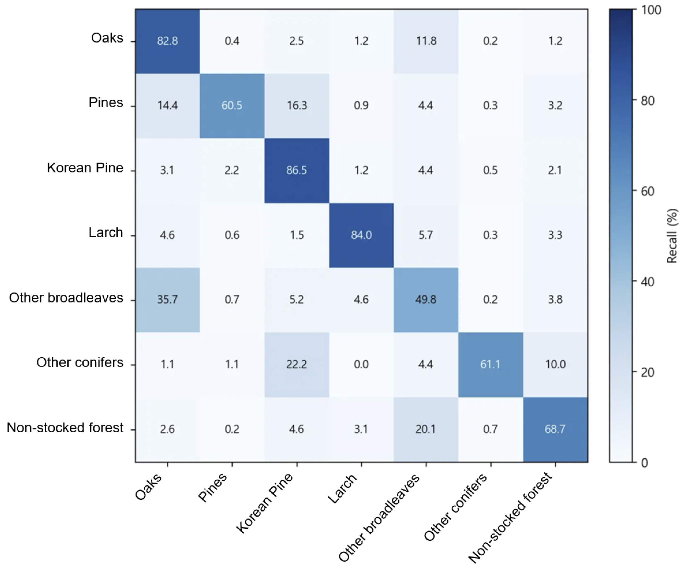
The full confusion matrix (3-run mean, row-normalized to recall) is presented in Appendix A (Figure A1). It indicates that most disagreements involved mutual confusion between oaks and other broadleaves (35.7% of other broadleaves predicted as oaks and 11.8% of oaks predicted as other broadleaves); pines were frequently predicted as Korean pine (16.3%) or oaks (14.4%), other conifers as Korean pine (22.2%), and non-stocked forest as other broadleaves (20.1%). The recall of other broadleaves also varied across replicates (0.50 ± 0.12; Table 2), a possible consequence of the spectral and phenological heterogeneity of this residual class, which includes several broadleaf genera.
3.2. Image-Based Mismatch Rate
3.2.1. Label Interpretation
Across all 501 interpreted stands, all three interpreters returned the same verdict on 47% of stands, and pairwise agreement ranged from 61% to 65% (Fleiss’ κ = 0.31, 95% CI 0.25–0.36). Among stands that no interpreter marked unsure, κ was 0.39. Interpreters differed in their use of the unsure category (78, 19, and 21 stands, respectively), but the remaining disagreement also indicates uncertainty in image-based assessment. Majority vote resolved 471 stands (94%); the remaining 30 were assigned through consensus adjudication. Subsequent analyses used these consolidated verdicts, with individual-interpreter results reported separately (Appendix E).
3.2.2. Flagged, Control, and Ungated Stands
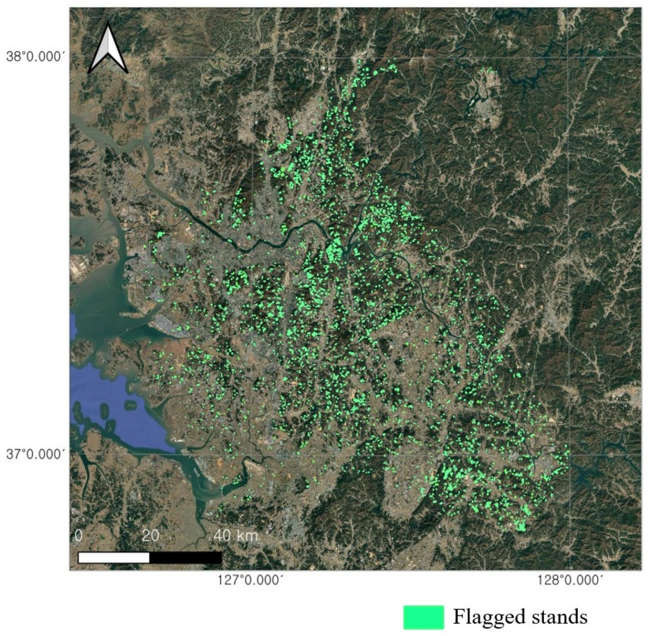
Applying the flag definition across the study region yielded 4303 flagged stands at the operating point (conf ≥ 0.70), representing 3.69% of all evaluable stands, of which 3248 fell in high-precision classes (Figure 3). The flagged pool contracted as the threshold increased, reaching approximately one-third of its size between conf ≥ 0.60 and conf ≥ 0.80 (Table 3).
Figure 3.
Spatial distribution of flagged stands. Green polygons indicate flagged stands. Polygon boundaries are enlarged for visualization purposes.
Table 3.
Number of flagged stands and percentages by confidence threshold in the study region.
At the operating point, 265 stands were interpreted across three gated groups: 94 high-precision-class flags, 79 controls, and 92 low-precision-class flags. Twelve stands received an unsure verdict (2, 1, and 9 respectively) and were excluded, leaving 253 resolved stands (match + mismatch). High-precision-class flags were mismatched substantially more often than controls among the interpreted stands: 38/92 (41.3%; 95% CI 31.8–51.5) versus 6/78 (7.7%; 95% CI 3.6–15.8), an odds ratio of 8.4 (95% CI 3.3–21.4; Fisher’s exact p = 4.2 × 10⁻⁷). This excess was not driven by any single class. Broken down by model-predicted class, all five high-precision classes exceeded the control rate, ranging from 33.3% (larch and oaks) to 58.8% (pines), and each contrast was significant (Fisher’s exact p = 9.5 × 10⁻⁶ to 1.5 × 10⁻²; Table 4). The contrast also persisted at alternative precision thresholds: recomputing the contrast at precision bounds of 0.55 and 0.65 yielded high-precision-class mismatch rates that remained well above that of the control at both bounds (0.361–0.429 vs. 0.077; Appendix C, Table A2).
Table 4.
Image-based mismatch rates by group and model-predicted class. Resolved N counts stands with match or mismatch verdicts. Rates and Wilson 95% confidence intervals are unweighted except those marked ᵃ, which are population-weighted estimates with stratified normal-approximation intervals (Section 2.4.3).
Contrary to our expectations, the low-precision-class flags did not resemble the controls. Their mismatch rate (41/83, 49.4%; 95% CI 38.9–59.9) was far above the mismatch rate of control (Fisher’s exact p = 3.1 × 10⁻⁹) and not significantly different from that of the high-precision-class flags (p = 0.29). However, this rate concealed two classes that behaved in opposite ways. Non-stocked forest, the class with the lowest measured precision of all seven (0.42), produced the highest mismatch rate in the study: 26/28 (92.9%; 95% CI 77.4–98.0). Other conifers, with a higher measured precision (0.55), produced the lowest mismatch rate of the seven: 15/55 (27.3%; 95% CI 17.3–40.2). The pooled rate of 49.4% therefore obscures the difference between the two classes. Both classes nonetheless exceeded the control rate (Fisher’s exact p = 7.4 × 10⁻¹⁷ and 3.3 × 10⁻³), so the precision stratification did not provide the expected prioritization in the primary analysis (Table 4).
Ungated stands were sampled by simple random sampling; of the 96 stands, three received an “unsure” verdict, leaving 93 resolved stands, of which 19 were mismatched (20.4%; 95% CI 13.5–29.7). Within this stratum, the two sources agreed on 36 stands and disagreed on 57. Agreeing stands were mismatched at 8.3% (3/36), which was close to the control rate of 7.7%. Disagreeing stands that fell below the threshold were mismatched at 28.1% (16/57), which was well above the rate of control but below the rates observed in both gated flag groups.
Estimating population mismatch rates from the interpreted sample requires weighting because pair-level caps resulted in overrepresentation of flags involving non-stocked forests. These flags accounted for 30.3% of the 175 interpreted flags but only 14.0% of the 4303 flagged stands. Weighting each flag type to its population (Section 2.4.3) resulted in an overall mismatch rate of approximately 35% (95% CI 26.4–43.6) for the flagged population. This pooled rate is used as the flagged-stratum input to the region-wide estimate, while differences between the two flag types are reported separately in Section 3.2.4. Weighted in the same manner, the high-precision-class flag rate was 29.7%, below its sample proportion of 41.3%, because the most common high-precision confusion pair in the population was undersampled and had a low mismatch rate. Combining the flagged, control, and ungated strata by their population sizes, with the control stratum post-stratified by map-dominant class, then yielded an estimated mismatch rate of 17.3% (95% CI 11.3–23.2) across the total 116,709 evaluable stands. Post-stratification lowered the control-stratum mismatch rate from the sample proportion of 7.7% to 5.9% (95% CI 1.1–10.7), because the control sample, which was matched to the flags, under-represented pines, which make up 32.8% of the control population and yielded no mismatch among the 15 interpreted stands. The estimate was insensitive to the rate assumed for the 1600 unsampled low-precision agreement stands (17.2%–17.5% for assumed rates of 0%–25%). Based on the mismatch types recorded during interpretation, this overall rate comprised 10.7% species-dominance mismatches and 6.6% stocking-status mismatches (Table 4).
3.2.3. Sensitivity Analysis
Confidence threshold. The same interpreted sample was reaggregated at lower confidence bounds from 0.60 to 0.80. Across this range the high-precision-class mismatch rate remained essentially stable (0.41–0.44), whereas the control rate fell monotonically as the threshold rose (0.123 → 0.077 → 0.037 → 0.000). The two groups therefore became increasingly separated at higher confidence, and high-precision-class flags exceeded controls at every threshold tested (Fisher’s exact p < 10−5 throughout; Appendix B, Table A1).
Across interpreters. The high-precision-class–control contrast was reproduced in all three interpreters’ independent assessments (52.5% vs. 21.9%, p = 2.7 × 10⁻⁴; 52.7% vs. 16.5%, p = 1.0 × 10⁻⁶; and 38.7% vs. 15.4%, p = 1.0 × 10⁻³), with odds ratios of 3.5–5.7. Absolute mismatch rates varied among interpreters (Appendix E, Table A4).
Split provenance. Of the 405 gated stands interpreted across the full confidence range, 87 (21.5%) were assigned to training cells. At the operating point, high-precision-class flags had mismatch rates of 10/25 (40.0%) in training cells and 28/67 (41.8%) elsewhere (Fisher’s exact p = 1.00). Within training cells, flags also exceeded controls (10/25 vs. 2/22; OR = 6.7; p = 0.021). These results show that informative disagreements occurred even where map labels had been available during training. Because the analysis conditions on selection into the interpreted groups, it does not quantify how training-label memorization affected the overall frequency of disagreements or unflagged map discrepancies.
3.2.4. Partition by Flag Type and Type of Discrepancy
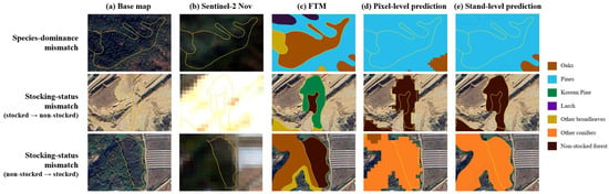
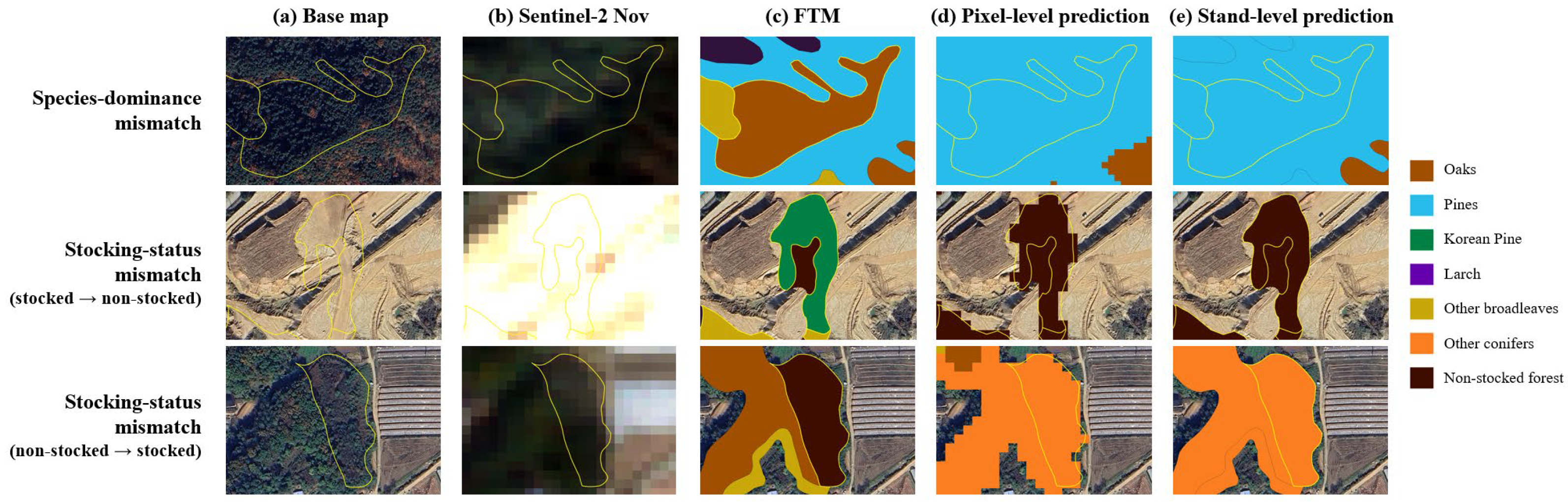
As the two low-precision classes behaved in opposite ways, the flagged stands were repartitioned based on whether the disagreement involved non-stocked forests in either direction (Table 5). Of the 175 flagged stands in the high-confidence analysis set, 122 showed species-to-species disagreements and 53 involved non-stocked forests (examples in Figure 4). The two flag types separated sharply: 39 of 122 species-dominance flags were mismatched, compared with 40 of 53 stocking-status flags, corresponding to an odds ratio of 6.55 (95% CI 3.15–13.62; Fisher’s exact p = 1.6 × 10⁻⁷). Among species-dominance flags, however, the precision strata did not differ significantly: 27 of 79 high-precision-class flags were mismatched, compared with 12 of 43 other conifer flags (odds ratio 1.34, 95% CI 0.60–3.02; Fisher’s exact p = 0.55), while both mismatch rates exceeded that of the control.
Table 5.
Image-based mismatch rates among flagged stands by flag type. Resolved N counts stands with match or mismatch verdicts. Rates marked ᵃ are population-weighted, with stratified normal-approximation intervals (Section 2.4.3); all other rates and Wilson intervals are unweighted. The corresponding unweighted rates for species-dominance and stocking-status flags are 39/122 (32.0%) and 40/53 (75.5%). All p values are two-sided Fisher’s exact tests against controls using unweighted counts.
Figure 4.
Representative confirmed mismatches by flag type. Yellow lines indicate the stand boundaries. Columns show (a) the high-resolution basemap, (b) a representative November 2025 Sentinel-2 composite, (c) the FTM, (d) pixel-level U-Net predictions, and (e) stand-level predictions. Row 1 shows a species-dominance mismatch, with the stand mapped as oaks but predicted as pines. Rows 2 and 3 show stocking-status mismatches in opposite directions: a stand mapped as Korean pine but predicted as non-stocked, and a stand mapped as non-stocked but predicted as other conifers, respectively.
Population-level mismatch rates were estimated using weights because the interpreted flags over-represented stocking-status disagreements and, among species-dominance flags, under-represented the most common confusion pair (mapped as other broadleaves, predicted as oaks), which accounted for 1172 of the 3700 species-dominance flags (31.7%), but only 8 of the 122 interpreted flags, of which only one was mismatched. Species-dominance flags accounted for 3700 of the 4303 flagged stands (86.0%), whereas stocking-status flags accounted for 603 (14.0%); weighted to their populations, the mismatch rates were 27.0% (95% CI 17.1–36.9) and 83.3% (95% CI 75.1–91.5) respectively, compared with unweighted sample proportions of 32.0% and 75.5%. Restricting each flag type to mismatches of its corresponding mismatch type yielded rates of 26.0% and 80.9%, respectively. Compared with region-wide rates of 10.7% for species-dominance mismatches and 6.6% for stocking-status mismatches, these rates corresponded to enrichments of 2.4-fold and 12.3-fold, respectively, over inspections drawn at random from the evaluable population.
4. Discussion
4.1. Model–Map Dominance Disagreement Is Enriched for Image–Map Mismatches
Stand-level agreement with the FTM was 0.69 by stand count and 0.76 area-weighted. Screening performance is evaluated through the concentration of image–map mismatches among flags. The ablation showed that bands and vegetation indices achieved agreement comparable to the full input, suggesting an opportunity to simplify implementation. Adding texture did not improve agreement, while topography recovered much of the decrease observed with texture. The net gain of the full set over bands and indices was small. The original 76-channel model was retained for the screening analysis to preserve the correspondence between the flag population and the interpretation sample. Whether the 51-channel bands-and-indices configuration preserves screening yield remains to be evaluated.
Blinded image interpretation found more mismatches among high-precision-class flags than controls in the interpreted sample (41.3% vs. 7.7%; OR = 8.4). This odds ratio is conditional on the selected sample composition. Population-level interpretation instead uses the weighted estimates, including 29.7% for high-precision-class flags (Section 3.2.2). The flag–control contrast persisted across individual interpreters and the tested confidence thresholds, and was also observed within training cells. These checks support the sample-based contrast under the tested choices; they do not remove dependence arising from supplementary use of the model-input imagery.
The controls were selected for model–map agreement and were partially matched to flag composition within the represented map classes. They therefore provide a comparison with agreeing stands, not a random-inspection baseline or a causal estimate holding composition fully constant. No comparison with other prioritization methods, such as disturbance-based screening, was conducted. The region-wide weighted estimate of 17.3%, which draws most of its weight from randomly sampled ungated stands, provides the relevant baseline for estimated inspection yield. Thus, the sample contrast evaluates whether disagreement carries information, while the weighted baseline estimates how much screening could increase yield in the evaluable population.
4.2. The Precision Criterion Is Not a Test of Flag Validity
Test-set class precision did not provide the expected prioritization in the primary analysis. Low-precision-class flags were mismatched at 49.4%, compared with 41.3% for high-precision-class flags (p = 0.29). The low-precision group combined non-stocked forest, with a mismatch rate of 92.9%, and other conifers, with 27.3%. Its pooled rate therefore obscures differences between the constituent classes and their flag-type composition. These findings do not support excluding a flag solely because its predicted class has low map-based precision. Flag type provides an alternative, exploratory basis for organizing review (Section 4.4).
4.3. Circular Dependence Between the Training Reference and the Audit Target, and Revision Lag
The FTM supplies both the training labels and the reference used to evaluate the classifier. Consequently, a correct prediction that departs from an erroneous map label is scored as a model error, whereas a prediction reproducing that label may agree with the map for the wrong reason. Imperfect reference data can bias agreement-based performance measures, with the direction depending on the association between reference and model errors [35]. These effects can also distort assignment to precision strata. Class precision here is a measure conditional on the FTM, not an independent measure of vegetation-classification reliability.
The training-cell comparison shows that the model did not reproduce all map labels even in areas represented during training. It does not rule out correlated errors within classes or estimate the fraction of map discrepancies missed because the model reproduced them. The interpretation results therefore support screening utility for the examined flags without resolving the full extent of dependence between model and map.
Changes between map production and image acquisition may partly explain the low map-based precision of non-stocked forest. The regional revision schedule places the most recent full-cycle revision in 2023, approximately two years before the 2025 imagery [1]. This scheduled revision year does not establish the observation date of every stand, particularly where subsequent updates have been incorporated. Harvesting after mapping could leave a species label over open ground, while regeneration could produce tree cover in a stand mapped as non-stocked. Of 28 flags predicted as non-stocked against a mapped species, 26 were judged mismatched; in the reverse high-precision direction, 11 of 13 were mismatched. These results demonstrate high image–map discrepancy rates in the sampled directions. They are consistent with the proposed temporal mechanisms but do not establish when the discrepancies arose or exclude original mapping errors.
4.4. Exploratory Organization by Flag Type
In the interpreted sample, mismatch rates were 32.0% for species-dominance flags (39/122) and 75.5% for stocking-status flags (40/53; OR = 6.55; Fisher’s exact p = 1.6 × 10⁻⁷). Population-weighted estimates were 27.0% and 83.3%, respectively. Interpreters recorded a mismatch type corresponding to the flag type in 74 of 79 mismatched stands, supporting the distinction between these screening channels. After stocking-status flags were removed, high- and low-precision species-dominance flags had rates of 34.2% and 27.9% (p = 0.55), and both exceeded controls.
Both flag types can reflect original mapping errors or subsequent change; the interpretation protocol cannot attribute their timing or origin. Harvesting and regeneration are plausible explanations for stocking-status mismatches, while species-dominance mismatches may also reflect compositional change. The elevated mismatch rate was not confined to stocking-status flags: high-precision-class species-dominance flags still exceeded controls (p = 5.8 × 10⁻⁵). The flag-type partition was developed after the pre-specified precision comparison and is exploratory. Its apparent value for prioritization requires confirmation with an independently drawn sample.
4.5. Operational Implications
Operational yield is estimated from the population-weighted rates. Stocking-status flags yielded corresponding stocking-status mismatches at 80.9%, compared with a region-wide baseline of 6.6%, giving 12.3-fold enrichment. Species-dominance flags yielded corresponding species-dominance mismatches at 26.0%, compared with a baseline of 10.7%, giving 2.4-fold enrichment. Under equal per-stand inspection effort, these estimates imply about 1.2 stocking-status flags or 3.8 species-dominance flags inspected per corresponding mismatch, compared with 15.2 or 9.3 randomly selected stands, respectively. These are expected yields inferred from image interpretation.
Stocking-status flags are a candidate first priority when inspection capacity is limited, given their higher estimated yield. Species-dominance flags can be retained as a separate queue and may complement disturbance-based screening by identifying compositional discrepancies without a detected canopy disturbance. Coverage was nevertheless partial: applying the estimated regional rate to the evaluable population implies approximately 20,000 mismatched stands, of which the flags captured about 1500 (7.5%). The output therefore supports targeted verification within a broader map-update process.
Ungated disagreements also contained potential mismatches. Among sampled stands that failed either the dominance or confidence gate, disagreeing stands were mismatched at 28.1% (16/57), compared with 8.3% (3/36) where model and map agreed. Because either gate could fail, these are ungated disagreements rather than a confidence-only subgroup. Their nonzero yield suggests that extending review beyond the gated pool could recover additional mismatches.
Raising the confidence threshold from 0.70 to 0.80 reduced the flagged pool from 4303 to 1555 stands, while high-precision-class mismatch proportions in the interpreted sample remained between 0.41 and 0.44. Thus, a stricter confidence gate reduced the candidate pool without a clear increase in this sample proportion. Weighted yield and coverage were not estimated separately at every threshold, so these results do not identify an optimal cutoff for a fixed budget. Threshold selection should balance the number of candidates against expected yield and the capacity for verification.
4.6. Limitations and Future Work
First, image interpretation was uncertain. Fleiss’ κ was 0.31, conventionally described as fair [36], and rose to 0.39 in the subset without unsure verdicts. Interpreter variability and uncertain reference labels are recognized issues in remote-sensing validation and classification [37,38,39,40]. Absolute mismatch rates differed among the individual interpreters, although the high-precision-class–control contrast remained significant in all three assessments (Appendix E). The primary analysis used majority vote and consensus adjudication to obtain consolidated verdicts. Absolute rates and the region-wide estimate of 17.3% should therefore be read as image-based estimates conditional on those verdicts.
Second, the results apply to one region and map vintage. Some discrepancies, particularly within broadleaf groups, may be difficult to resolve with 10 m imagery and image interpretation. The heterogeneous other-broadleaves class is a possible contributor to confusion with oaks, and their most common flag pair yielded few confirmed mismatches. Stand-specific observation dates underlying the map labels were not established in this study, and the relationship between time since mapping and mismatch rates was not assessed. Evaluation across regions and mapping vintages would help assess transferability.
Third, sampling was designed for the precision strata rather than the later flag-type partition. Species-dominance flags comprised 86% of the flagged population but had a sampling fraction of only 3.3%, producing a wide weighted interval (17.1%–36.9%). The pair mapped as other broadleaves and predicted as oaks comprised 32% of species-dominance flags but had only eight interpretations. Population estimates depend on the weighting scheme and on resolved interpretations representing the weighting strata, including the broader groups used for stocking-status flags. They also require an assumed rate for 1600 unsampled agreeing stands in low-precision classes; varying that rate from 0% to 25% changed the region-wide estimate by less than half a percentage point.
Fourth, several choices remain incompletely evaluated. Although model-fitting and test data were separated by spatial cells, the statistical tests on interpreted stands treated stands as independent. Spatial dependence may affect significance tests and uncertainty estimates and was not explicitly evaluated. Excluding boundary pixels increased map agreement by about three percentage points, but the stability of the flag set and interpretation yield under buffering was not tested. Image availability and interpretation introduce additional uncertainty. Basemap acquisition dates were uncontrolled, and supplementary use of the Sentinel-2 model inputs may introduce correlated errors whose effects need not be equal across groups. At 89% of stand representative points, the September composite had at most two valid observations (Appendix F); these counts describe observation availability, not residual cloud contamination or all within-stand gaps. The effects of alternative seasonal combinations were not evaluated. The cell-selection and flagging criteria also require further assessment. The visual cell-exclusion procedure involves judgement, and sensitivity to the 10% threshold was not assessed. Robustness to this cutoff has therefore not been established. Test-set agreement therefore describes the selected cells, while the effect of this selection rule on region-wide screening performance remains uncertain. Sensitivity to the 0.70 dominance cutoff should also be assessed in further studies.
5. Conclusions
This study found that stand-level disagreement between a Sentinel-2 U-Net classifier and the FTM can identify stands worth verifying in the study region. High-precision-class flags had more image–map mismatches than controls in the interpreted sample (41.3% vs. 7.7%; OR = 8.4). Test-set class precision did not provide the expected prioritization under the primary analysis. An exploratory partition by flag type showed different weighted yields: corresponding stocking-status mismatches occurred in 80.9% of stocking-status flags and corresponding species-dominance mismatches in 26.0% of species-dominance flags, giving enrichments of 12.3-fold and 2.4-fold over their respective regional baselines.
The flag types offer candidate queues for verification, with stocking-status flags showing the higher estimated yield and species-dominance flags retaining a distinct role. Approximately 35% of flagged stands were estimated to be mismatches, but the flags captured only about 7.5% of estimated regional mismatches. These findings support targeted inspection before map edits within a broader updating process. The framework uses public satellite data and the existing map and could support pre-screening of zones scheduled for revision. Its yield and the proposed flag-type priorities require evaluation in additional regions and an independently drawn validation sample.
Supplementary Materials
The following supporting information can be downloaded at: https://www.mdpi.com/article/10.3390/f17111294/s1, Supplementary Material S1: Model implementation details; Table S1: Vegetation indices computed per seasonal composite; Table S2: GLCM texture features (B8, 7 × 7 window, distance 1, four directions averaged); Table S3: Allocation of fishnet cells to splits for the first replicate and subsequent analysis; Table S4: Training hyperparameters and configuration.
Author Contributions
Conceptualization, H.L. (Heejae Lee); methodology, H.L. (Heejae Lee); validation, H.L. (Heejae Lee) and S.-E.C.; formal analysis, H.L. (Heejae Lee); investigation, H.L. (Heejae Lee) and H.L. (Hyunjin Lee); resources, E.-S.K. and C.-R.P.; data curation, H.L. (Heejae Lee) and H.L. (Hyunjin Lee); writing—original draft preparation, H.L. (Heejae Lee); writing—review and editing, S.-E.C., E.-S.K. and C.-R.P.; visualization, H.L. (Heejae Lee); supervision, S.-E.C.; project administration, S.-E.C.; funding acquisition, C.-R.P. All authors have read and agreed to the published version of the manuscript.
Funding
This research was funded by the National Institute of Forest Science, Republic of Korea, grant number FE0100-2026-04-2026.
Data Availability Statement
Data are available from the corresponding author upon request.
Conflicts of Interest
The authors declare no conflicts of interest.
Abbreviations
The following abbreviations are used in this manuscript:
| CI | Confidence interval |
| DEM | Digital elevation model |
| FAO | Food and Agriculture Organization of the United Nations |
| FGIS | Forest Geospatial Information System |
| FTM | Forest type map |
| GLCM | Gray-level co-occurrence matrix |
| LCMAP | Land Change Monitoring, Assessment, and Projection |
| OR | Odds ratio |
| SD | Standard deviation |
| USGS | United States Geological Survey |
Appendix A. Confusion Matrix
Figure A1.
Confusion matrix for stand-level classification, averaged over three replicate runs and row-normalized to recall (%). Rows show FTM reference classes; columns show model predictions.
Appendix B. Sensitivity to the Confidence Threshold
The interpreted stands with conf ≥ 0.60 were re-partitioned at lower confidence bounds from 0.60 to 0.80. Because interpretation was performed once on the full sample, varying the threshold re-partitioned already-interpreted stands; no additional stands were interpreted.
Table A1.
Sensitivity of the high-precision-class versus control contrast to the model confidence threshold.
Appendix C. Sensitivity to the Class-Precision Bound
The primary analysis defined model-predicted classes with test-set precision ≥ 0.60 as high-precision classes. Sensitivity was assessed by repeating the high-precision-class-versus-control comparison (conf ≥ 0.70) at precision bounds of 0.55, 0.60, and 0.65, while holding the originally sampled control group fixed. Relaxing the bound to 0.55 included other conifers, whereas tightening it to 0.65 excluded oaks; non-stocked forest remained in the low-precision stratum throughout. The contrast with the control remained significant at all bounds (Table A2).
Table A2.
Sensitivity of the high-precision-vs-control contrast to the precision bound (conf ≥ 0.70; control held fixed).
Appendix D. Sensitivity of Agreement to the Predictor Set
The predictor groups were evaluated with four nested input sets under the training configuration in Table S4. Each set was trained three times with different initialization seeds and evaluated on the same 5797 test stands. These runs held cell allocation fixed (Table S3), whereas the main replicates varied model initialization and training-cell selection while keeping the test cells fixed; their variability therefore summarizes a different source of variation. Bands and indices slightly increased agreement over bands alone. Adding texture reduced agreement, while topography recovered much of that decrease; the full set showed little net gain over bands and indices (Table A3). This experiment evaluates map agreement, not the comparative screening yield of the reduced inputs.
Table A3.
Stand-level agreement with the FTM by predictor set (mean ± SD, three runs).
Appendix E. Variation Among Interpreters
The primary analysis assigned final labels by majority vote, with consensus adjudication for stands on which all three interpreters differed. To assess variation among interpreters, Table A4 compares group mismatch rates from each interpreter’s independent verdicts with the primary consolidated labels. Unsure verdicts were excluded separately in each assessment, so resolved sample sizes differ among interpreters and from the primary analysis. These comparisons describe variation in unweighted sample rates; population-weighted regional estimates were based on the consolidated labels.
Table A4.
Mismatch rates by group for the primary analysis and individual interpreters (conf ≥ 0.70; mismatched/resolved stands, % in parentheses).
Appendix F. Valid Observations in the Seasonal Composites
For each seasonal composite, the number of valid observations per pixel was computed as the number of scenes in which the pixel was not masked by the scene classification layer (cloud shadow, medium- and high-probability cloud, cirrus, and snow), among scenes with less than 50% cloudy pixels. Values were sampled at a representative point of each of the 235,788 FTM stands in the study region. Observation counts differed little among classes (Table A5); these counts do not directly measure residual cloud contamination or all within-stand gaps. Spatial differences were larger: the median per 4 × 4 km cell ranged from 4 to 29 in April, from 0 to 7 in September, and from 2 to 21 in November, with higher values in areas covered by adjacent orbits. In September, the cell median was one or fewer in 106 of the 566 cells.
Table A5.
Valid observations at stand representative points by seasonal composite and class (median, with the 5th percentile in parentheses), and percentages of representative points with two or fewer valid observations.
References
- Korea Forest Service. Forest Type Map. Available online: https://www.forest.go.kr/newkfsweb/html/HtmlPage.do?pg=/fgis/UI_KFS_5002_020100.html&mn=KFS_02_04_03_04_01&orgId=fgis (accessed on 13 July 2026).
- Decuyper, M.; Chávez, R.O.; Lohbeck, M.; Lastra, J.A.; Tsendbazar, N.; Hackländer, J.; Herold, M.; Vågen, T.-G. Continuous monitoring of forest change dynamics with satellite time series. Remote Sens. Environ. 2022, 269, 112829. [Google Scholar] [CrossRef] [Scilit]
- Fuller, D.O. Tropical forest monitoring and remote sensing: A new era of transparency in forest governance? Singap. J. Trop. Geogr. 2006, 27, 15–29. [Google Scholar] [CrossRef] [Scilit]
- Molnár, T.; Király, G. Forest disturbance monitoring using cloud-based Sentinel-2 satellite imagery and machine learning. J. Imaging 2024, 10, 14. [Google Scholar] [CrossRef] [Scilit]
- Lister, A.J.; Andersen, H.; Frescino, T.; Gatziolis, D.; Healey, S.P.; Heath, L.S.; Liknes, G.C.; McRoberts, R.; Moisen, G.G.; Nelson, M.; et al. Use of remote sensing data to improve the efficiency of national forest inventories: A case study from the United States national forest inventory. Forests 2020, 11, 1364. [Google Scholar] [CrossRef] [Scilit]
- Grabska-Szwagrzyk, E.; Tymińska-Czabańska, L. Sentinel-2 time series: A promising tool in monitoring temperate species spring phenology. For. Int. J. For. Res. 2024, 97, 267–281. [Google Scholar] [CrossRef] [Scilit]
- Grabska, E.; Hostert, P.; Pflugmacher, D.; Ostapowicz, K. Forest stand species mapping using the Sentinel-2 time series. Remote Sens. 2019, 11, 1197. [Google Scholar] [CrossRef] [Scilit]
- Fassnacht, F.E.; Latifi, H.; Stereńczak, K.; Modzelewska, A.; Lefsky, M.; Waser, L.T.; Straub, C.; Ghosh, A. Review of studies on tree species classification from remotely sensed data. Remote Sens. Environ. 2016, 186, 64–87. [Google Scholar] [CrossRef] [Scilit]
- Mouret, F.; Morin, D.; Planells, M.; Vincent-Barbaroux, C. Tree species classification at the pixel level using deep learning and multispectral time series in an imbalanced context. Remote Sens. 2025, 17, 1190. [Google Scholar] [CrossRef] [Scilit]
- Liu, P.; Ren, C.; Wang, Z.; Jia, M.; Yu, W.; Ren, H.; Xia, C. Evaluating the potential of Sentinel-2 time series imagery and machine learning for tree species classification in a mountainous forest. Remote Sens. 2024, 16, 293. [Google Scholar] [CrossRef] [Scilit]
- Lee, J.; Yang, T.; Choi, C. Mapping nine dominant tree species in the Korean peninsula using U-Net and harmonic analysis of Sentinel-2 imagery. Korean J. Remote Sens. 2025, 41, 243–260. [Google Scholar] [CrossRef] [Scilit]
- Lee, H.; Lee, C.; Woo, H.; Choi, S.-E. Optimal training sample sizes for U-Net-based tree species classification with Sentinel-2 imagery. Forests 2025, 16, 1718. [Google Scholar] [CrossRef] [Scilit]
- Wulder, M.A.; Hermosilla, T.; White, J.C.; Bater, C.W.; Hobart, G.; Bronson, S.C. Development and implementation of a stand-level satellite-based forest inventory for Canada. For. Int. J. For. Res. 2024, 97, 546–563. [Google Scholar] [CrossRef] [Scilit]
- Oliver, C.D.; Larson, B.C. Forest Stand Dynamics, Update ed.; John Wiley & Sons: New York, NY, USA, 1996. [Google Scholar]
- Maas, A.E.; Rottensteiner, F.; Heipke, C. A label noise tolerant random forest for the classification of remote sensing data based on outdated maps for training. Comput. Vis. Image Underst. 2019, 188, 102782. [Google Scholar] [CrossRef] [Scilit]
- Ren, M.; Zeng, W.; Yang, B.; Urtasun, R. Learning to reweight examples for robust deep learning. In Proceedings of the 35th International Conference on Machine Learning (ICML 2018), Stockholm, Sweden, 10–15 July 2018; PMLR: New York, NY, USA, 2018; Volume 80, pp. 4334–4343. [Google Scholar]
- Northcutt, C.; Jiang, L.; Chuang, I. Confident learning: Estimating uncertainty in dataset labels. J. Artif. Intell. Res. 2021, 70, 1373–1411. [Google Scholar] [CrossRef] [Scilit]
- Paris, C.; Bruzzone, L. A novel approach to the unsupervised extraction of reliable training samples from thematic products. IEEE Trans. Geosci. Remote Sens. 2021, 59, 1930–1948. [Google Scholar] [CrossRef] [Scilit]
- Northcutt, C.G.; Athalye, A.; Mueller, J. Pervasive label errors in test sets destabilize machine learning benchmarks. In Proceedings of the Neural Information Processing Systems Track on Datasets and Benchmarks; Neural Information Processing Systems Foundation, Inc.: San Diego, CA, USA, 2021; Volume 1. [Google Scholar]
- Tan, Y.; Sun, K.; Wei, J.; Gao, S.; Cui, W.; Duan, Y.; Liu, J.; Zhou, W. STFNet: A spatiotemporal fusion network for forest change detection using multi-source satellite images. Remote Sens. 2024, 16, 4736. [Google Scholar] [CrossRef] [Scilit]
- Khankeshizadeh, E.; Mohammadzadeh, A.; Moghimi, A.; Mohsenifar, A. FCD-R2U-Net: Forest change detection in bi-temporal satellite images using the recurrent residual-based U-net. Earth Sci. Inform. 2022, 15, 2335–2347. [Google Scholar] [CrossRef] [Scilit]
- Rynkiewicz, A.; Hościło, A.; Aune-Lundberg, L.; Nilsen, A.B.; Lewandowska, A. Detection and quantification of vegetation losses with Sentinel-2 images using bi-temporal analysis of spectral indices and transferable random forest model. Remote Sens. 2025, 17, 979. [Google Scholar] [CrossRef] [Scilit]
- Radoux, J.; Defourny, P. Automated image-to-map discrepancy detection using iterative trimming. Photogramm. Eng. Remote Sens. 2010, 76, 173–181. [Google Scholar] [CrossRef] [Scilit]
- Wang, J.; Xia, X.; Lan, L.; Wu, X.; Yu, J.; Yang, W.; Han, B.; Liu, T. Tackling noisy labels with network parameter additive decomposition. IEEE Trans. Pattern Anal. Mach. Intell. 2024, 46, 6341–6354. [Google Scholar] [CrossRef] [Scilit]
- Yang, H.; Yao, Q.; Han, B.; Kwok, J.T. Searching to exploit memorization effect in deep learning with noisy labels. IEEE Trans. Pattern Anal. Mach. Intell. 2024, 46, 7833–7849. [Google Scholar] [CrossRef] [Scilit]
- Gorelick, N.; Hancher, M.; Dixon, M.; Ilyushchenko, S.; Thau, D.; Moore, R. Google Earth Engine: Planetary-scale geospatial analysis for everyone. Remote Sens. Environ. 2017, 202, 18–27. [Google Scholar] [CrossRef] [Scilit]
- Korea Forest Service. Forest Geographic Information Service. Available online: https://map.forest.go.kr/forest/ (accessed on 27 February 2026).
- Boeing, G. Modeling and analyzing urban networks and amenities with OSMnx. Geogr. Anal. 2025, 57, 567–577. [Google Scholar] [CrossRef] [Scilit]
- OpenStreetMap Contributors. OpenStreetMap. Available online: https://www.openstreetmap.org (accessed on 15 May 2026).
- FAO. FRA 2000: On Definitions of Forest and Forest Change; Forest Resources Assessment Programme Working Paper 33; FAO: Rome, Italy, 2000; Available online: https://www.fao.org/4/ad665e/ad665e00.htm (accessed on 23 July 2026).
- Ronneberger, O.; Fischer, P.; Brox, T. U-Net: Convolutional networks for biomedical image segmentation. In Medical Image Computing and Computer-Assisted Intervention—MICCAI 2015, Proceedings of the 18th International Conference, Munich, Germany, 5–9 October 2015; Navab, N., Hornegger, J., Wells, W.M., Frangi, A.F., Eds.; Springer International Publishing: Cham, Switzerland, 2015; Volume 9351, pp. 234–241. [Google Scholar] [CrossRef] [Scilit]
- Cochran, W.G. Sampling Techniques, 3rd ed.; John Wiley & Sons: New York, NY, USA, 1977. [Google Scholar]
- Wilson, E.B. Probable inference, the law of succession, and statistical inference. J. Am. Stat. Assoc. 1927, 22, 209–212. [Google Scholar] [CrossRef]
- Fleiss, J.L. Measuring nominal scale agreement among many raters. Psychol. Bull. 1971, 76, 378–382. [Google Scholar] [CrossRef] [Scilit]
- Foody, G.M. Assessing the accuracy of land cover change with imperfect ground reference data. Remote Sens. Environ. 2010, 114, 2271–2285. [Google Scholar] [CrossRef] [Scilit]
- Landis, J.R.; Koch, G.G. The measurement of observer agreement for categorical data. Biometrics 1977, 33, 159–174. [Google Scholar] [CrossRef] [Scilit]
- Stehman, S.V.; Mousoupetros, J.; McRoberts, R.E.; Næsset, E.; Pengra, B.W.; Xing, D.; Horton, J.A. Incorporating interpreter variability into estimation of the total variance of land cover area estimates under simple random sampling. Remote Sens. Environ. 2022, 269, 112806. [Google Scholar] [CrossRef] [Scilit]
- Van Coillie, F.M.B.; Gardin, S.; Anseel, F.; Duyck, W.; Verbeke, L.P.C.; De Wulf, R.R. Variability of operator performance in remote-sensing image interpretation: The importance of human and external factors. Int. J. Remote Sens. 2014, 35, 754–778. [Google Scholar] [CrossRef] [Scilit]
- Pelletier, C.; Valero, S.; Inglada, J.; Champion, N.; Marais Sicre, C.; Dedieu, G. Effect of training class label noise on classification performances for land cover mapping with satellite image time series. Remote Sens. 2017, 9, 173. [Google Scholar] [CrossRef] [Scilit]
- Pengra, B.W.; Stehman, S.V.; Horton, J.A.; Dockter, D.J.; Schroeder, T.A.; Yang, Z.; Cohen, W.B.; Healey, S.P.; Loveland, T.R. Quality control and assessment of interpreter consistency of annual land cover reference data in an operational national monitoring program. Remote Sens. Environ. 2020, 238, 111261. [Google Scholar] [CrossRef] [Scilit]

Disclaimer/Publisher’s Note: The statements, opinions and data contained in all publications are solely those of the individual author(s) and contributor(s) and not of MDPI and/or the editor(s). MDPI and/or the editor(s) disclaim responsibility for any injury to people or property resulting from any ideas, methods, instructions or products referred to in the content. |
© 2026 by the authors. Licensee MDPI, Basel, Switzerland. This article is an open access article distributed under the terms and conditions of the Creative Commons Attribution (CC BY) license.