


Abstract
Rapid urban expansion into mountainous terrain, together with increasing exposure to extreme weather, has increased the need for transparent and interpretable slope-hazard assessment in forested and residential mountain environments. However, relatively few studies have integrated field-survey information with physically based simulation outputs for interpretable multi-class classification within an established slope-hazard grading framework. This pilot study developed a simulation-informed machine-learning framework for classifying composite slope-hazard grades (Grades I–III) using 71 landslide-prone and 52 debris-flow-prone sites in Sejong City, Republic of Korea. For the landslide dataset, selected field-survey indicators were integrated with SoilWorks-derived slope-stability information, whereas for the debris-flow dataset, selected field-survey indicators were integrated with FLO-2D-derived simulation information. Four machine-learning algorithms—Random Forest (RF), Logistic Regression (LR), K-Nearest Neighbors (KNN), and Support Vector Machine (SVM)—were evaluated under severe class imbalance. RF showed the strongest overall performance in the original holdout evaluation, achieving an accuracy of 0.857 for both datasets and weighted F1-scores of 0.849 for the landslide dataset and 0.836 for the debris-flow dataset. Repeated stratified train–test analyses further showed that RF retained the highest mean overall performance, although the debris-flow dataset was more sensitive to sample allocation. Gini importance, Shapley Additive Explanations (SHAP), and targeted ablation analysis indicated that simulation-derived variables provided strong discriminatory information within the established grading framework. The proposed framework provides a structured and interpretable approach for integrating field-based assessment indicators with physically based simulation outputs and may provide supplementary support for classifying and prioritizing sites requiring further assessment. The findings also provide a basis for future investigation of reduced-input screening approaches, although the present study does not establish that reduced field surveys or simulation outputs alone are sufficient for formal grade assignment. Accordingly, the framework should be interpreted as a supplementary classification approach within the existing assessment system rather than as an independent predictor of future landslide or debris-flow occurrence.
1. Introduction
Landslides and debris flows are major natural hazards in mountainous regions worldwide, often resulting in significant economic losses, infrastructure disruption, and casualties [1,2,3,4,5]. These hazards are controlled by a variety of predisposing factors, including morphology, lithology, geological structure, vegetation, and land use, and may be triggered by prolonged rainfall, typhoons, seismic activity, or anthropogenic disturbances [6,7,8,9]. In some cases, landslides can evolve into or supply material to debris flows, in which saturated soil and unconsolidated materials mobilize rapidly along steep channels [10].
With the intensification of climate change, extreme weather events are becoming more frequent and severe, exacerbating slope instability in vulnerable areas. Simultaneously, rapid urban expansion into mountainous terrain has emerged as an important anthropogenic factor affecting slope hazards. Activities such as slope cutting, deforestation, road construction, and land-use transformation can alter hillside environments and increase the likelihood and potential consequences of slope failure, particularly in densely populated or newly developed mountain-edge urban zones [11,12,13].
Within such mountainous environments, forest vegetation can further influence slope conditions through both surface protection and root reinforcement [14]. Vegetation cover can reduce surface erosion, while root systems may increase soil cohesion and shear resistance and thereby contribute to slope stability [15]. Conversely, forest degradation, vegetation loss, or shallow-rooted conditions may reduce these protective functions and increase susceptibility to erosion and shallow instability [14]. These vegetation-related conditions are relevant not only to landslide-prone slopes but also to debris-flow processes, because shallow landslides can supply sediment to channel networks and, under suitable conditions, transform into rapidly moving debris flows [16]. Such interactions are particularly important where residential development is expanding into forested and mountainous terrain.
The Republic of Korea provides a relevant setting for examining these interactions, with mountains covering approximately 63% of its territory [17]. Sejong City, centrally located in the Republic of Korea, has undergone rapid development as a planned administrative city, with urban expansion extending into surrounding hilly and mountainous terrain [18]. With elevations ranging from approximately 30 to 700 m, the city contains complex relief and slopes adjacent to residential areas. During the monsoon season, intense rainfall combined with these terrain conditions can increase susceptibility to landslides and debris flows. These characteristics make Sejong City a useful case study for slope-hazard assessment in rapidly urbanizing mountainous environments.
Against this background, slope-hazard assessment requires consideration of multiple interacting factors, including topographic conditions, soil properties, vegetation, hydrological conditions, land use, and the potential exposure of residential areas and infrastructure. Several studies have highlighted the importance of residential and public infrastructure vulnerability in mountainous hazard assessment [19,20,21,22]. Machine-(ML) methods provide a means of evaluating complex and potentially nonlinear relationships among multiple predictors, while interpretable approaches can further help clarify the relative contributions of individual variables to classification results. Such approaches can complement established slope-assessment frameworks by providing an additional data-driven perspective on multi-factor hazard classification.
In response to these challenges, machine-learning methods have gained prominence in landslide susceptibility mapping and slope-hazard assessment. A range of algorithms, including Random Forest (RF), Logistic Regression (LR), K-Nearest Neighbors (KNN), Extreme Gradient Boosting (XGB), and Support Vector Machines (SVMs), have been applied to model relationships among topographic, hydrological, environmental, and anthropogenic variables [23,24,25,26,27]. For example, Wang et al. [23] compared RF and frequency-ratio approaches for landslide susceptibility mapping in Chongqing, China; Pham et al. [24] evaluated hybrid machine-learning approaches for landslide susceptibility assessment; and Lee and Pradhan [25] applied frequency-ratio and logistic-regression models for landslide hazard mapping in Selangor, Malaysia. These studies demonstrate the broad applicability of data-driven approaches to slope-hazard assessment, although their objectives, target definitions, and modeling frameworks differ.
However, many previous studies have focused primarily on landslide susceptibility assessment and mapping using binary landslide/non-landslide classification schemes [23,24,25,26,27]. Recent studies have begun to explore multi-class approaches. For example, Zhang et al. [28] proposed a statistical knowledge-guided multi-class machine-learning scheme for landslide susceptibility levels. Nevertheless, comparatively fewer studies have examined multi-class slope-hazard grading involving both landslide- and debris-flow-prone sites, particularly in mountainous residential areas characterized by complex terrain and rapid land development. Furthermore, limited attention has been paid to simultaneously evaluating classification performance, robustness under class imbalance, and model interpretability within an established slope-hazard grading framework.
Beyond developments in multi-class modeling, the integration of physics-based or numerical simulation with data-driven machine learning has also received increasing attention. Han and Semnani [29] integrated outputs from the TRIGRS and SHALSTAB physics-based models into machine-learning-based landslide susceptibility assessment, while Gao et al. [30] combined FLO-2D numerical simulations with a gradient-boosted decision tree model for debris-flow hazard mapping. These studies illustrate the potential of simulation–machine-learning integration; however, their objectives and integration strategies differ from those of the present study. The combined use of field-survey indicators and simulation-derived variables within an interpretable multi-class grading framework for both landslide- and debris-flow-prone sites remains comparatively less explored.
To address these gaps, this study develops a simulation-informed machine-learning framework for multi-class slope-hazard classification (Grades I–III) in mountainous residential areas. The target grades are defined within an established assessment framework that combines a field-assessment component with simulation- or stability-based evaluation, as summarized in Table 1 [31]. These composite slope-hazard grades are distinct from conventional landslide-susceptibility classes and from probabilistic risk estimates because they incorporate field-survey conditions, damage- and exposure-related information, and simulation-based evaluation. Separate but parallel classification analyses are conducted for landslide-prone and debris-flow-prone sites. For the landslide dataset, selected field-survey variables are integrated with SoilWorks-derived slope-stability information, whereas for the debris-flow dataset, selected field-survey variables are integrated with FLO-2D-derived simulation information.
Table 1.
Description of slope hazard grades based on composite assessment scores from field evaluation and simulation (0–100 scale).
Because the established grades can be formally assigned from the complete composite assessment score, the purpose of machine learning in this study is not to replace the existing scoring rules. Rather, it is used to examine how effectively a selected subset of field-survey and simulation-derived information can discriminate among the established Grade I–III classes and to identify which predictors contribute most strongly to this classification. The final composite score itself is not used as an input predictor; however, some of the field-survey and simulation-derived variables used as predictors also contribute to construction of the target grades. Accordingly, model performance is interpreted as classification performance within the established grading framework rather than as independent prediction of future landslide or debris-flow occurrence.
Four representative machine-learning algorithms—Random Forest (RF), Logistic Regression (LR), K-Nearest Neighbors (KNN), and Support Vector Machine (SVM)—are evaluated because they represent different modeling assumptions and have been widely applied in landslide and slope-hazard studies [23,24,25,26,27,32,33]. In addition to classification performance, this study emphasizes model interpretability using Gini importance and Shapley Additive Explanations (SHAP). Gini importance provides a global measure of predictor contribution within tree-based models, while SHAP offers a game-theoretic framework for quantifying feature contributions at both global and class-specific levels [34,35]. Together, these approaches provide complementary information on how individual predictors contribute to multi-class slope-hazard classification.
Therefore, the objectives of this study are threefold: (1) to develop multi-class classification models for established landslide and debris-flow slope-hazard grades in residential mountain-edge areas; (2) to evaluate and compare the classification performance and robustness of four machine-learning algorithms under conditions of class imbalance; and (3) to interpret the relative contributions of field-survey and simulation-derived variables using Gini importance, SHAP-based feature attribution, and targeted ablation analysis.
The study area, Sejong City, a planned administrative city in central Republic of Korea, represents a rapidly urbanizing mountainous environment characterized by strong seasonal rainfall and ongoing land development. The resulting classification framework may provide supplementary information for classifying and prioritizing slope-hazard sites requiring further assessment, with potential relevance to forested-slope management, spatial planning, infrastructure protection, and disaster-risk management in similar mountainous regions. From a broader sustainability perspective, such slope-hazard assessment and management efforts are also relevant to the United Nations Sustainable Development Goal 11 (Sustainable Cities and Communities), particularly Targets 11.5 and 11.b concerning disaster-impact reduction, urban resilience, and integrated disaster-risk management [36]. Given the limited sample size and localized spatial scope, the present study is designed as a pilot investigation of simulation-informed machine learning for multi-class slope-hazard classification within the established assessment framework. The study area and the spatial distribution of the assessed landslide-prone and debris-flow-prone sites are shown in Figure 1.
Figure 1.
Overview of the study area and locations of the landslide-prone and debris-flow-prone assessment sites in Sejong City, Republic of Korea. In the main map, blue lines represent streams. The green-to-yellow/orange background provides topographic context, while the lower-right inset shows satellite imagery of the study area.
2. Materials and Methods
2.1. Study Area and Hazard Assessment Design
Sejong City is a centrally located, planned administrative capital of Republic of Korea, officially established in 2012 [37]. While the urban core area is relatively flat, surrounding residential development zones frequently extend into hilly and mountainous terrain [18]. As the city expands, many slopes are subjected to anthropogenic disturbances such as excavation, road cutting, and deforestation, all of which contribute to increasing slope instability.
Due to the ongoing expansion of Sejong City into both hillside and valley environments, the study area presents two distinct types of slope hazard environments: (1) landslides occurring on or near man-modified hillslopes adjacent to residential areas, and (2) debris flows developing along narrow valleys or stream channels, typically triggered by rainfall-induced runoff and sediment mobilization.
To capture these differing hazard mechanisms, this study adopts a dual-component assessment strategy, separating landslide-prone areas from debris-flow-prone areas based on topographic and hydrological features. This division allows for a more targeted analysis and better alignment between field survey protocols, simulation tools, and classification models.
This study, therefore, comprises two components: a Landslide Hazard Area Assessment for mountain slopes and a Debris-flow Hazard Area Assessment for mountain valleys or stream channels. Both assessment frameworks were based on field survey data and stability simulation results, following criteria established by the Republic of Korea Forest Service.
Specifically, the field-survey indicators were derived from the official site-survey assessment forms for landslide- and debris-flow-prone areas provided in the “Guidelines for Surveying Areas at Risk of Landslides and for the Designation and Management of Vulnerable Areas,” an administrative guideline established pursuant to Article 37-2 of the Enforcement Rules of the Forest Protection Act [31]. This regulation, under the jurisdiction of the Republic of Korea Forest Service, incorporates legally mandated guidelines and technical standards related to landslide and debris-flow hazard evaluation.
The study was conducted between 30 July 2019 and 29 July 2022. Survey sites were identified using spatial information, including the Korea Forest Service landslide hazard map, debris-flow damage prediction map, digital topographic data, and information on existing and planned development, followed by field investigation. In this study, a “site” refers to an individual field-assessment unit rather than to a recorded landslide or debris-flow event. Landslide sites represented assessed hillslope areas, whereas debris-flow sites represented assessed mountain-stream and associated catchment areas. In total, 71 landslide-prone sites and 52 debris-flow-prone sites were included in the analysis.
Each site was assigned a composite assessment score on a 0–100 scale according to the established slope-hazard assessment framework. The total score consisted of a field-assessment component of up to 70 points and a simulation- or stability-based component of up to 30 points. For landslide-prone sites, the 70-point field-assessment component comprised damage potential (15 points), topographic conditions (25 points), and key risk factors (30 points). For debris-flow-prone sites, the field-assessment component followed the same overall 70-point structure, comprising damage potential (15 points), topographic conditions (25 points), and risk factors (30 points).
For each site i, the composite assessment score was expressed as
where Si is the total composite assessment score (0–100), Fi is the complete field-assessment score (maximum 70 points) calculated according to the established assessment framework, and Mi is the corresponding simulation- or stability-based score (maximum 30 points).
Si = Fi + Mi
For landslide-prone sites, the SoilWorks-based slope-stability evaluation contributed 0, 15, or 30 points. A score of 0 was assigned when the prescribed factor-of-safety criterion was satisfied (FoS ≥ 1.6 under dry conditions or ≥1.3 under rainy conditions), 15 points when the FoS was within the borderline range (1.5–1.6 under dry conditions or 1.2–1.3 under rainy conditions), and 30 points when the criterion was not satisfied (FoS < 1.5 under dry conditions or <1.2 under rainy conditions). For debris-flow-prone sites, the FLO-2D simulation component likewise contributed 0, 15, or 30 points: 0 points when no exposed target was located within the simulated impact area, 15 points when property at risk was present, and 30 points when human or infrastructure exposure was present.
The resulting composite slope-hazard grade, Gi, was assigned according to the composite score Si using the thresholds specified in the established assessment framework (Table 1). These thresholds were not estimated or optimized using the present dataset. The final composite score Si itself was not used as an input predictor.
In addition, the machine-learning predictor set did not include all indicators used to calculate the complete field-assessment score Fi. Instead, the models used a selected subset of field-survey indicators together with simulation-derived variables, as summarized in Table 2. The predictor set was therefore not intended to reproduce the complete official scoring system deterministically. Nevertheless, because some of the predictors also contributed to the construction of the target grades, structural dependence remains between the predictor set and the target labels. Accordingly, model performance is interpreted as classification performance within the established grading framework rather than as independent prediction of future landslide or debris-flow occurrence.
Table 2.
Description of selected variables used in landslide and debris-flow hazard classification.
All input variables were divided into two groups: landslide-related variables and debris-flow-related variables. Continuous field measurements, including slope angle, slope height, soil depth, basin area, and channel slope, were categorized using the threshold values specified in the same assessment framework [31]. These thresholds were not derived from the present dataset, and the categorical representation was retained to maintain consistency with the field-assessment procedure used to construct the hazard grades. Because the objective of this study was to evaluate classification within the established grading framework, alternative discretization thresholds were not optimized or tested using the present dataset. Their definitions, categories, data sources, and contributions to the composite grading framework are summarized in Table 2.
Among these variables, Landslide Susceptibility Level serves as a foundational indicator in both the landslide and debris-flow models and therefore warrants additional explanation. This variable was classified into five categories based on the dominant susceptibility zone within each analysis unit. The classification was derived from spatial data provided by the Landslide Information System of the Korea Forest Service, which offers nationwide assessments of landslide-prone areas. The system assigns Susceptibility Levels 1 to 5, where Level 1 indicates very high susceptibility and Level 5 denotes minimal or no susceptibility. These levels are determined using both natural factors (e.g., slope, geology, soil moisture) and anthropogenic influences (e.g., roads, buildings, land use). Specifically, a unit is assigned: Level 1 when the majority of its area overlaps with Susceptibility Level 1 zones; Level 2 when more than 50% overlaps with Level 2; Level 3 when less than 50% corresponds to Level 2; Level 4 when most of the area falls within Level 3 or 4 zones; and Level 5 when the majority of the area corresponds to Level 5 (minimal or no susceptibility). However, for the debris-flow dataset, Level 4 was defined as areas where the majority of the unit overlapped with Susceptibility Levels 3 through 5, rather than only Levels 3 or 4. This adjustment reflects the broader spatial distribution of lower-susceptibility zones in debris-flow-prone areas. Because the national Landslide Susceptibility Level is derived from several environmental and anthropogenic factors, some of its information may overlap with other predictors used in the models. It was retained because it is an established indicator in the assessment framework. Therefore, its feature importance should be interpreted as predictive contribution within the model rather than as an independent causal effect.
The overall analytical framework integrating field-survey indicators, simulation-derived information, machine-learning model development, independent evaluation, and RF-based interpretation is summarized in Figure 2.
Figure 2.
Overall analytical framework for composite slope-hazard grade classification using field-survey indicators, simulation-derived information, and machine-learning models.
2.2. Landslide Dataset
2.2.1. Landslide-Related Damage Potential
The assessment of damage potential in the study sites was based on two main criteria: (1) whether damage events—such as landslides, infrastructure failures, or property loss—had occurred previously, and (2) whether protective facilities were present within the sphere of direct influence.
As shown in Figure 3a, the majority of sites were classified as having no recorded damage (87.3%) or indirect damage (12.7%). Notably, no sites were identified as having experienced direct damage (0%), indicating a relatively low historical impact in the assessed areas.
Figure 3.
Distribution of damage potential in the landslide hazard study area. (a) Damage history, and (b) exposed assets within the direct impact zone: A = none, B = property damage risk, C = small residential clusters, D = densely populated or infrastructure zones.
To quantify the potential impact of slope hazards, areas within the direct impact zone were categorized into four protective types (A–D), ranging from no facilities to densely populated areas with critical infrastructure (see Table 2 for details). As illustrated in Figure 3b, Type D accounted for the highest proportion at 49.3%, indicating a significant concentration of population and infrastructure in hazard-prone zones. Type B followed with 28.2%, while Type C and Type A accounted for 12.7% and 9.8%, respectively.
These findings emphasize that, although no direct damage events have been recorded at the surveyed sites, a significant proportion of the surveyed sites are situated in areas with high exposure—particularly those containing critical infrastructure and dense residential populations. This underscores the importance of implementing proactive hazard mitigation measures and comprehensive risk management strategies to reduce potential future impacts.
2.2.2. Topographic Characteristics of Landslide Sites
In this study, the topographic characteristics of soil slopes are analyzed based on four key parameters: slope angle, slope height, soil depth, and cross-sectional slope type. These factors play significant roles in slope stability and susceptibility to landslides.
The slope angle is a critical parameter as it directly influences the gravitational force acting on geomaterials deposited on a slope, thereby affecting the potential for slope failure [25]. As shown in Figure 4a, the slope angle was categorized into four classes. Slopes with angles between 0° and 25° were the most common, accounting for 71.8% of all surveyed sites. This indicates that gentle slopes are predominant in the study area.
Figure 4.
Topographic characteristics of landslide sites: (a) Slope angle; (b) slope height; (c) soil depth; and (d) cross-sectional type. °, degree; m, meter.
Regarding slope height, the sites were divided into five height categories. According to Figure 4b, slopes with a height greater than 40 m were the most frequent, comprising 33.8% of the total. This was followed by slopes of 5–20 m (25.3%), 20–30 m (23.9%), and 30–40 m (16.9%). The prevalence of high slopes suggests an increased potential for landslide activity, especially when combined with other triggering factors.
The soil depth was also divided into five categories. As depicted in Figure 4c, the most common depth range was 50–80 cm, representing 57.7% of the sites. Soil depths between 80 and 100 cm accounted for 23.9%. These values suggest a relatively deep soil profile, which could influence infiltration rates, water retention, and slope loading characteristics.
Finally, the cross-sectional slope types were classified into four categories. As illustrated in Figure 4d, the combined type was the most prevalent, accounting for 67.6%, followed by the parallel type at 26.8%. The dominance of complex slope geometries (combined types) may indicate varying stress distributions and water flow patterns, which could affect slope stability differently compared to uniform profiles.
2.2.3. Key Risk Factors in Landslide Hazard Assessment
The key risk factors affecting slope stability in this study include landslide susceptibility levels, water conditions, slope failure types, root characteristics, and forest conditions.
The Landslide Susceptibility Level was derived from the national landslide susceptibility zoning map of the Korea Forest Service, where Level 1 represents very high susceptibility and Level 5 denotes minimal or no susceptibility (see Section 2.1). Within the study area, as shown in Figure 5a, 56.3% of the area was classified as Level 1, indicating that more than half of the slope units are located in zones with very high susceptibility. A further 15.5% of the sites fell into Level 3 (moderate susceptibility), while 28.2% was classified as Level 4, representing relatively low susceptibility. No areas were mapped as Level 2 or Level 5. Overall, these patterns indicate that although some parts of the study area fall into lower-susceptibility classes, a substantial portion of slopes is still situated in highly susceptible zones that require careful monitoring and management.
Figure 5.
Key risk factors for slope instability: (a) landslide susceptibility level map; (b) water availability conditions; (c) slope failure types: A = none, B = surface or gully erosion, C = slope collapse, and D = rockfall or creeping failure; (d) root characteristics: A = mix, B = deep roots, C = shallow roots or non-forested area; (e) forest conditions: A = no standing trees B = high, C = low/medium, and D = deforested area; and (f) slope stability evaluation (SoilWorks): A = stable, B = borderline, and C = unstable.
Water availability conditions in the study area were categorized into four types (Table 2). As shown in Figure 5b, dry conditions accounted for 67.6% of the study area, while 32.4% of the sites were classified as humid. Surface water and spring water were not observed in the study area. The predominance of dry conditions suggests limited near-surface water availability, which may constrain vegetation growth and root development, potentially reducing slope reinforcement. In contrast, humid zones, although less extensive, may facilitate water infiltration into the soil, contributing to soil saturation and increasing the likelihood of slope failure in those areas. The absence of surface or spring water suggests that permanent concentrated water sources are not a dominant factor directly affecting slope stability at the surveyed sites.
Slope failure zones were classified into four types (Table 2). As shown in Figure 5c, 69.0% of the sites showed no visible slope failure (Type A), 29.6% exhibited surface or gully erosion (Type B), and 1.4% showed signs of slope collapse (Type C). No rockfall or creeping failure (Type D) was observed. The dominance of Type A indicates that most of the study area is currently stable with no visible signs of failure. However, the 28.2% of the sites affected by surface or gully erosion indicates ongoing soil degradation that could potentially lead to further slope instability. The 2.8% of the sites with slope collapse, although limited in extent, highlight localized zones where more detailed monitoring and mitigation are required.
Root characteristics of soil slopes were categorized into three types (Table 2). As shown in Figure 5d, 85.9% of the sites were classified as Type A, indicating a combination of shallow- and deep-rooted vegetation. A further 9.9% of the sites consisted of predominantly deep-rooted vegetation (Type B), while 4.2% comprised shallow-rooted vegetation or non-forested areas (Type C). The dominance of Type A suggests that most slopes are covered by mixed root systems, which can enhance slope stability by providing a complex root network. The presence of deep-rooted vegetation (Type B) in certain areas can further stabilize slopes, whereas areas with shallow-rooted vegetation or non-forested conditions (Type C) are more vulnerable to erosion and slope failure due to weaker root reinforcement.
Forest conditions were classified into four categories (Table 2). According to Figure 5e, 63.4% of the sites were categorized as Type B, indicating high canopy density and relatively dense vegetation cover that can contribute to slope stability. Around 25% of the sites were classified as Type C, representing forests with low to medium canopy density, and about 10% as Type D, corresponding to deforested or disturbed areas. Type A (No Standing Trees) accounted for a very small proportion and can be considered negligible. The significant presence of Types C and D indicates regions with reduced vegetation cover, which are more prone to soil erosion and slope instability. These areas warrant closer monitoring and potential restoration efforts to enhance vegetation cover and mitigate future hazards.
2.2.4. Slope Stability Evaluation
Slope stability was assessed using SoilWorks (version 2022 v1.1; MIDAS IT Co., Ltd., Seongnam, Republic of Korea), a widely adopted simulation tool in Korea. The analysis aimed to determine whether a slope could remain stable under external conditions such as rainfall, loading, or disturbance. The variable “evaluation” refers to the slope stability classification result generated from this simulation and serves as a key input in the landslide hazard modeling. Functionally, it is comparable to the “simulation” variable used in the debris-flow assessment, which was derived from FLO-2D.
The factor-of-safety (FoS)—defined as the ratio of shear strength to shear stress—was calculated based on input parameters from field investigations, including slope geometry and soil conditions.
Based on the calculated safety factor (FoS), slope stability was classified into three categories: Type A (Stable): FoS ≥ 1.6 (dry season) or ≥ 1.3 (rainy season), Type B (Borderline): FoS between 1.5 and 1.6 (dry) or 1.2 and 1.3 (rainy), Type C (Unstable): FoS < 1.5 (dry) or below the rainy season threshold. This classification allowed for clear identification of slopes requiring attention, with unstable and borderline cases highlighting potential areas for monitoring or mitigation.
As shown in Figure 5f, 60.6% of the sites fell under Type A, indicating general stability. However, 29.6% were classified as Type C, revealing potential risks under certain environmental conditions. Type B accounted for 9.9%, suggesting a small fraction of slopes are in a borderline state. These findings support the need for focused reinforcement or monitoring in less stable areas to prevent future slope failures.
2.3. Debris-Flow Data
2.3.1. Debris-Flow-Related Damage Potential
As part of the debris-flow hazard area assessment for mountain valleys and stream channels, the evaluation of damage potential at the study sites was conducted based on two primary criteria:(1) whether damage events—such as landslides, infrastructure failures, or property loss—had occurred previously, and (2) whether protective facilities were present within the sphere of direct influence.
As shown in Figure 6a, the results indicate that 73.1% of the sites exhibited no record of prior damage, while 17.3% experienced indirect damage, and 9.6% were directly impacted. These findings suggest that although the majority of sites have not been previously affected, a significant proportion remains vulnerable to potential future hazards.
Figure 6.
Distribution of damage potential in debris-flow hazard areas. (a) Damage history, and (b) exposed assets within the direct impact zone: A = none, B = property damage risk, C = small residential clusters, D = densely populated or infrastructure zones.
Protective facilities located within the directly impacted areas were classified into four categories (Table 2). As shown in Figure 6b, among these, Type D accounted for 65.4%, reflecting a predominant focus on safeguarding densely populated or infrastructure-sensitive regions. Type B and Type C followed, representing 19.2% and 15.4%, respectively. Type A was not observed, indicating that all directly impacted areas had at least some level of protective measures in place. This distribution highlights a risk-prioritized strategy, wherein resources are concentrated in areas of higher population density and critical social and economic value.
2.3.2. Topographic Characteristics of Debris-Flow Sites
The topographic conditions analyzed in this study include basin area, average slope angle, and soil depth, which are important factors in debris-flow risk.
As shown in Figure 7a, the basin area was divided into five groups. Most sites (40.4%) had a basin area between 6 and 10 ha, followed by 11–20 ha (34.6%) and less than 5 ha (15.4%). This means that medium-sized basins are common, which can collect enough water and sediment to trigger debris flows.
Figure 7.
Topographic characteristics of debris-flow sites: (a) basin area, (b) soil depth, and (c) average channel slope.
As shown in Figure 7b, the most common soil depth was 80–100 cm (46.2%), followed by 50–80 cm (34.6%). Shallow soils were less common. Deeper soils can absorb more water but may become unstable when saturated, potentially increasing susceptibility to slope instability and debris-flow initiation.
According to Figure 7c, most debris-flow channels (59.6%) had an average channel slope between 5° and 15°, followed by channels with slopes less than 5° (32.7%) and those between 15° and 20° (7.7%). No channels were steeper than 20°. These results indicate that moderate slope gradients dominate the surveyed valleys, which may facilitate debris-flow mobility during intense rainfall events.
Overall, the results show that most sites have medium basin sizes, moderate slopes, and deep soil layers, which are conditions that may lead to debris flows, especially during strong or continuous rainfall events.
2.3.3. Key Risk Factors in Debris-Flow Hazard Assessment
The key risk factors considered in the debris-flow hazard assessment include landslide susceptibility level, forest condition, and root characteristics.
As shown in Figure 8a, Level 1 was the most common, representing 65.4% of the sites, followed by Level 4 at 21.2%. Given that Level 1 indicates very high susceptibility and higher levels correspond to lower susceptibility (Section 2.1), these patterns suggest that a substantial proportion of debris-flow-prone sites are located in high-susceptibility zones, although some areas fall into relatively lower-susceptibility categories.
Figure 8.
Key risk factors influencing debris-flow susceptibility: (a) landslide susceptibility level map, (b) forest condition: A= high canopy, B = low/medium canopy, C = fallen trees and dead trees, and D = deforested or degraded area, (c) root characteristics: A = mix, B = shallow C = deep, and (d) debris-flow impact level (FLO-2D): A = no impact, B = asset risk, and C = human/infrastructure risk.
The forest condition was divided into four types (Table 2). According to Figure 8b, Type A accounted for 34.6% of sites, while Type B and Type C made up 32.7% and 30.8%, respectively. This suggests that although many sites are well-forested, a significant number show signs of forest degradation, which may increase slope vulnerability.
The root system characteristics were grouped into three categories (Table 2). As shown in Figure 8c, Type A was dominant (84.6%), while Type B and Type C were less common, at 1.9% and 13.5%, respectively. The presence of mixed rooting systems in most areas likely contributes positively to slope reinforcement and stability.
Overall, the results indicate that many debris-flow-prone sites are located in zones with high mapped landslide susceptibility but are generally supported by relatively strong root systems. However, where forest conditions are degraded or canopy cover is reduced, slope stability may be compromised, increasing the likelihood of debris-flow initiation and propagation. Such vegetation-related conditions may therefore warrant closer consideration in field-based debris-flow assessment and slope management.
2.3.4. Debris-Flow Simulation-Based Hazard Evaluation
Debris-flow hazard was assessed using the FLO-2D model (Build 21; FLO-2D software, Inc., Nutrioso, AZ, USA), a grid-based two-dimensional simulation tool. This model is widely used for evaluating sediment transport and flood behavior in mountainous terrains [38]. The model was selected for its ability to realistically simulate debris-flow movement based on topographic and hydrologic inputs. Model inputs, including flow depth, basin slope, and sediment concentration, were derived from field data and topographic maps. In this study, model parameters were calibrated using field data and topographic maps to enhance simulation accuracy. Based on the simulation results, the impact level of debris flows was classified into three categories: Type A (no impact): no affected targets within the debris-flow range; Type B (asset risk): presence of vulnerable properties (e.g., farmland); Type C (human/infrastructure risk): presence of people or critical infrastructure (e.g., residential clusters, roads).
As shown in Figure 8d, Type B zones accounted for the largest proportion (71.2%), followed by Type C (17.3%) and Type A (11.5%). These results suggest that although direct impacts on human life are relatively rare, a significant number of areas face risks to property or infrastructure, highlighting the importance of prioritizing mitigation measures in Type B and C zones.
2.4. Data Preprocessing and Balancing
Data preprocessing. A series of preprocessing procedures was applied to ensure the quality and suitability of the landslide and debris-flow datasets for multi-class classification.
Missing data imputation. Across the two databases, only one missing value was identified in the feature related to landslide hazard level. This missing value was imputed using the mode of the corresponding variable.
Encoding variables. A total of 12 features from the landslide dataset and 9 features from the debris-flow dataset were selected as input variables for model development. To make the datasets compatible with machine learning algorithms, appropriate encoding methods were applied. The target variable “grade”, originally labeled as “Grade I”, “Grade II”, and “Grade III”, was converted into a numeric factor (0, 1, and 2, respectively). Several variables, including slope angle, slope height, soil depth, basin area, hazard level, evaluation, and simulation, were represented as ordinal categories with a natural order and were therefore encoded as integers according to their ranked values. In contrast, unordered categorical variables—including damage type, protection type, cross-sectional shape, presence of water, slope failure type, forest condition, and other nominal categorical variables—were transformed using one-hot encoding, generating binary indicator variables for each category without introducing artificial order.
Data partitioning. The datasets were split into training and test sets in a 6:4 ratio while maintaining class stratification. For the debris-flow dataset, the extremely small number of Grade III instances (only two sites) required manual allocation: one Grade III site was assigned to the training set and one to the test set to ensure that all classes were represented. Samples for Grades I and II were then randomly assigned according to the specified ratio.
Class balancing. To address class imbalance in the training set, the Synthetic Minority Oversampling Technique (SMOTE) was applied with k = 5 for both datasets to generate synthetic samples for minority classes [39]. For the debris-flow dataset, the training data were grouped into Grade III versus the remaining classes (Grades I–II). SMOTE (k = 5) was applied to Grades I and II, whereas the single available Grade III training sample was oversampled by simple replication, being repeated 20 times. As a result, the balanced debris-flow training set combined synthetic SMOTE-generated samples for Grades I–II with replicated samples for Grade III. Because all replicated Grade III cases originate from a single site, the effective diversity of training data for this class remains low and the resulting Grade III performance should be interpreted with caution. The numbers of observations in each slope-hazard grade for the original training set, balanced training set, and independent test set are summarized in Table 3.
Table 3.
Class distributions of the original training, balanced training, and test sets for the landslide and debris-flow datasets.
Feature selection. Near-zero-variance and highly sparse predictors were identified from the training data and removed before model fitting. The same predictor columns were subsequently excluded from the corresponding test set to maintain consistency and avoid using test information during feature selection.
These preprocessing steps helped to reduce noise, mitigate data imbalance, and enhance the stability of the subsequent classification models.
2.5. Machine Learning Model Setup and Evaluation
2.5.1. Model Selection and Training Procedures
Random Forest (RF) is an ensemble tree-based learning algorithm capable of modeling nonlinear relationships and complex interactions among predictors and has been widely applied in landslide susceptibility and hazard studies [23,27,40]. RF is also known for its strong predictive performance and robustness across classification tasks [41]. Classification is based on majority voting across multiple decision trees [42,43]. In this study, RF was implemented using the randomForest package (vesion 4.7-1.1) in R (version 4.2.1; R Foudation for Statistical Computing, Vienna, Austria). The key hyperparameter, mtry, which determines the number of predictors randomly sampled at each split, was optimized by grid search with cross-validation. The selected values were mtry = 6 for the landslide dataset and mtry = 4 for the debris-flow dataset.
Logistic Regression (LR) is a generalized linear modeling approach widely used for classification, including landslide susceptibility and hazard assessment [25,44]. For multi-class classification, multinomial logistic regression extends binary logistic regression to more than two outcome classes. In this study, multinomial logistic regression was implemented using the glmnet method in the caret package (version 6.0-93). The regularization parameters alpha and lambda were optimized by grid search with cross-validation. The selected values were alpha = 0 (ridge regression) and lambda = 0.001 for both datasets.
K-Nearest Neighbors (KNN) is a non-parametric, instance-based learning algorithm that assigns observations to classes according to the classes of their nearest neighbors in predictor space [45,46,47]. In this study, KNN was implemented using the caret package in R. The number of neighbors, k, was optimized by cross-validation, with selected values of k = 3 for the landslide dataset and k = 11 for the debris-flow dataset.
Support Vector Machine (SVM) is a supervised learning method suitable for high-dimensional and nonlinear classification and has been applied in landslide, slope-stability, and geohazard studies [32,33,48,49]. It can model nonlinear relationships through kernel functions and is recognized for its strong generalization performance and resistance to overfitting [3]. In this study, a Gaussian radial basis function (RBF) kernel was used [33]. The RBF-SVM has two key hyperparameters: the penalty parameter C and the kernel parameter sigma. The parameter C controls the penalty associated with misclassification, whereas sigma determines the influence range of training observations in the RBF kernel [33]. The SVM model was implemented using the svmRadial method in the caret package in R. Both C and sigma were optimized by grid search with 5-fold cross-validation using the training data. For the landslide dataset, candidate values for both C and sigma ranged from 2−2 to 22, and the selected values were C = 4 and sigma = 0.25. For the debris-flow dataset, a broader tuning grid was used, with C ranging from 2−2 to 26 and sigma from 2−10 to 20. The parameter combination yielding the highest cross-validated accuracy within the training data was selected, resulting in C = 0.25 and sigma = 0.25. The resulting tuned models were subsequently evaluated on the corresponding independent test sets.
2.5.2. Model Evaluation Metrics
The target variable in this study consists of three ordinal categories (Grade I, Grade II, and Grade III) with a highly imbalanced distribution, particularly with only one independent Grade III observation in the test set of the debris-flow dataset. Due to this imbalance, standard accuracy is not a reliable performance metric. Instead, we focused on metrics that account for class imbalance and provide a balanced evaluation across all classes. Specifically, we employed the following metrics:
Macro-averaged Precision, Recall, and F1-score: These metrics assign equal weight to each class regardless of class frequency, thereby providing a class-balanced summary of model performance across the three slope-hazard grades.
Weighted-averaged Precision, Recall, and F1-score: These metrics account for class frequency and provide an overall evaluation that reflects the observed class distribution.
Cohen’s Kappa: A measure of agreement between the model-predicted grades and the observed grade labels in the independent test set, adjusted for agreement expected by chance. Kappa was calculated separately for each model. Kappa was retained as a complementary metric because, unlike overall accuracy, it adjusts the observed agreement for the agreement expected from the marginal class distributions, which is particularly relevant under severe class imbalance.
Overall Accuracy: Reported as a complementary metric but not used alone to assess model performance because of its sensitivity to class imbalance.
All metrics were calculated using the independent test set, which retained the original class distribution. For classes with no positive predictions, undefined class-wise precision and F1-score were assigned a value of zero. All three target classes were therefore retained in the calculation of macro-averaged metrics. The same zero-contribution treatment was applied consistently when calculating weighted-average metrics.
To examine the sensitivity of model performance to the specific train–test allocation, the stratified 6:4 train–test partitioning procedure was repeated 50 times using different sample allocations. For each repetition, all preprocessing, class-balancing, feature-filtering, and hyperparameter-tuning procedures were conducted using the training data only, followed by evaluation on the corresponding independent test set. For the debris-flow dataset, one of the two independent Grade III observations was retained in the training set and the other in the test set in each repetition. Training-set performance was additionally calculated using the original, non-synthetic training observations to facilitate comparison with independent test-set performance.
2.6. Model Interpretation: Feature Importance and SHAP
2.6.1. Gini-Based Feature Importance
To assess the relative contribution of each input variable to the RF classification results, feature importance was quantified using Gini importance (i.e., Mean Decrease in Gini impurity). Among the evaluated models, RF was selected for interpretability analysis because it achieved the highest overall accuracy in both the landslide and debris-flow datasets and provides a tree-based framework suitable for variable-importance analysis. Gini importance reflects the cumulative reduction in node impurity attributable to each predictor across the fitted trees. Higher values therefore indicate a greater contribution to distinguishing the composite slope-hazard grades within the fitted RF model. These importance values were used for relative ranking of predictors and were not interpreted as evidence of causal effects.
2.6.2. SHAP-Based Feature Attribution
Shapley Additive Explanations (SHAP), grounded in cooperative game theory, provides a unified approach to model interpretation and has been increasingly applied in geological-hazard modeling to quantify feature contributions [34,35]. In this study, SHAP analysis was applied to the RF models for landslide and debris-flow classification in Sejong City, using the fastshap package (version 0.07) in R to compute mean absolute SHAP values. These values summarize the magnitude of each predictor’s contribution to the model output and complement the global rankings obtained from Gini importance [43]. Due to the small sample size and class imbalance, particularly the limited number of Grade III observations in the debris-flow dataset, directional SHAP values showed inconsistent trends across classes and were therefore interpreted cautiously [50]. Accordingly, mean absolute SHAP values were primarily used to rank the relative contributions of predictors to the RF classification results. Because a subset of the field-survey indicators and simulation-derived variables also contributed to the construction of the target grades, high Gini or SHAP importance was interpreted as strong discriminatory influence within the established grading framework rather than as independent evidence of physical causality or improved predictive accuracy.
2.7. Targeted Ablation Analysis
To further examine the contribution of the simulation-derived variables and the Landslide Susceptibility Level, a targeted ablation analysis was conducted using the RF model. Four predictor scenarios were evaluated separately for each dataset: (1) the full predictor set; (2) the predictor set excluding the simulation-derived variable; (3) the predictor set excluding the Landslide Susceptibility Level; and (4) the predictor set excluding both variables. For the landslide dataset, the simulation-derived variable corresponded to the SoilWorks-derived slope-stability evaluation variable, whereas for the debris-flow dataset it corresponded to the FLO-2D-derived simulation variable.
The ablation analysis used 50 repeated stratified 6:4 train–test partitions. For each repetition and predictor scenario, preprocessing, class balancing, feature filtering, and RF hyperparameter tuning were performed using the training data, followed by evaluation on the corresponding independent test set. Performance was summarized using accuracy, weighted F1-score, macro F1-score, and Cohen’s Kappa across the 50 repetitions.
3. Results
3.1. Comparison of Model Performance
To compare the classification performance of different machine-learning models, four algorithms—RF, LR, KNN, and SVM—were applied separately to the landslide and debris-flow datasets. Their performance was evaluated using accuracy, precision, recall, F1-score, and Cohen’s Kappa. Class-wise metrics were also examined to assess the ability of each model to distinguish among the three slope-hazard grades (Grades I–III).
3.1.1. Landslide Hazard Classification
As summarized in Table 4, RF showed the strongest overall performance for the landslide dataset. It achieved the highest accuracy (0.857) and weighted F1-score (0.849). Its macro precision (0.847), macro recall (0.867), and macro F1-score (0.828) also indicated relatively balanced performance across the three grades. The corresponding Cohen’s Kappa was 0.765.
Table 4.
Test-set performance of four models for the landslide dataset.
Among the remaining models, Logistic Regression yielded moderate performance, with an accuracy of 0.786 and a macro F1-score of 0.764. KNN performed the worst among the models in terms of overall accuracy (0.679), with a macro F1-score of 0.624. The SVM model showed mixed performance, with an accuracy of 0.750 and a weighted-average F1-score of 0.702, but a lower macro F1-score (0.536) and macro recall (0.586), reflecting uneven performance across classes.
Class-wise results in Table A1 further support these observations. RF consistently performed well across all slope-hazard grades, particularly with F1-scores of 0.800 (Grade I), 0.750 (Grade II), and 0.933 (Grade III). Notably, the SVM model failed to identify any Grade I observations; under the evaluation procedure described in Section 2.5.2, its precision and F1-score for this class were therefore assigned a value of 0.
3.1.2. Debris-Flow Hazard Classification
For the debris-flow dataset, performance results are summarized in Table 5. Among the four models, again, RF achieved the highest overall accuracy (0.857) and a strong weighted-average F1-score (0.836), together with the highest Kappa value (0.642). Its macro F1-score was 0.568. RF performed well for Grades I and II (F1 = 0.800 and 0.903, respectively), but failed to identify the single Grade III test observation, resulting in a recall of 0 and precision and F1-score values of 0 for that class (Table A1).
Table 5.
Test-set performance of four models for the debris-flow dataset.
The SVM model showed comparatively weak performance in the debris-flow dataset, with an accuracy of 0.714, a weighted F1-score of 0.595, and a macro F1-score of 0.278. Although its accuracy was 0.714, the SVM predicted all 21 test observations as Grade II. Because Grade II accounted for 15 of the 21 observed test labels, the observed agreement (15/21 = 0.714) was equal to the agreement expected from the marginal class distributions, resulting in a Cohen’s Kappa of 0.000. This indicates that the apparently moderate accuracy was driven by prediction of the majority class rather than balanced discrimination among the three debris-flow grades, particularly the minority class.
Logistic Regression also achieved an accuracy of 0.810, with a macro F1-score of 0.556, macro precision and recall both at 0.556, and a Kappa value of 0.558. KNN achieved an accuracy of 0.571 and a weighted F1-score of 0.597, with a macro F1-score of 0.519 and Kappa of 0.315. It showed the highest macro recall (0.756) among the four models. Notably, KNN was the only model that successfully identified the Grade III test observation (recall = 1.000), although its low precision (0.200) and F1-score (0.333) indicate substantial uncertainty in the classification of this sparsely represented class (Table A1).
Despite differences between the two datasets, RF showed the strongest overall performance based on accuracy, weighted F1-score, and Cohen’s Kappa. Its class-wise performance was relatively consistent for the landslide dataset, whereas performance for the debris-flow Grade III class remained limited. Logistic Regression achieved comparatively strong overall accuracy in the debris-flow dataset, whereas SVM and KNN showed lower overall performance and weaker macro-averaged metrics.
To assess the robustness of these results to the specific train–test allocation, the stratified 6:4 partitioning procedure was repeated 50 times, with model hyperparameters re-tuned within the training data for each repetition. For the landslide dataset, RF showed the highest mean performance across all four principal evaluation metrics, with an accuracy of 0.861 ± 0.066, weighted F1-score of 0.857 ± 0.070, macro F1-score of 0.849 ± 0.084, and Kappa of 0.768 ± 0.111. RF achieved the highest weighted and macro F1-scores in 44 of the 50 repeated partitions. For the debris-flow dataset, RF likewise showed the highest mean accuracy (0.741 ± 0.062), weighted F1-score (0.719 ± 0.057), macro F1-score (0.471 ± 0.086), and Kappa (0.353 ± 0.136). However, model rankings varied more across debris-flow partitions, with RF achieving the highest weighted F1-score in 32 of 50 repetitions and the highest macro F1-score in 25 of 50 repetitions. These results indicate greater sensitivity of the debris-flow models to sample allocation, although RF retained the strongest average overall performance (Table A2).
Overall, among the four models evaluated in this study, RF provided the strongest overall classification performance for both landslide and debris-flow hazard grading.
3.2. Feature Importance Analysis
Feature importance analysis was performed to examine the relative contribution of each predictor to the classification of composite slope-hazard grades. Gini importance (Mean Decrease in Gini impurity) was calculated from the RF models to provide a global ranking of predictor contributions [33]. Feature importance analysis was conducted using the Gini importance (i.e., Mean Decrease in Gini impurity) from the RF models, which consistently exhibited strong overall performance across both landslide and debris-flow datasets. This helps highlight the most influential variables in hazard classification.
For the landslide dataset (Figure 9), the top-ranked feature was “evaluation,” which refers to the slope stability classification generated by SoilWorks based on the factor of safety (FoS). This indicates its strong contribution to distinguishing landslide hazard grades within the RF model. The next most important features were “failure_none” and “failure_erosion,” indicating that the presence or absence of observable slope failures substantially influenced model predictions. Additional important features included “protect_dense” and “slope_height,” indicating the contribution of both exposure-related and topographic factors.
Figure 9.
Gini importance (Mean Decrease Gini) for the landslide and debris-flow RF models. In the landslide model, ‘evaluation’ (SoilWorks’ slope stability classification, based on the factor of safety) is the top-ranked feature, indicating its strong contribution to landslide grade classification. In the debris-flow model, ‘simulation’ (FLO-2D’s impact level, based on flow depth and sediment concentration) is the top-ranked feature, indicating its strong contribution to debris-flow grade classification. Other highly ranked features, such as ‘failure_none’ and ‘soil_depth’, also contribute to the respective classification results. See Table 2 for detailed feature definitions.
In the debris-flow dataset, the most important feature was “simulation,” which was derived from FLO-2D modeling results, indicating its strong contribution to debris-flow grade classification. Other highly ranked variables included “soil_depth,” “protect_cluster,” and “hazard_level,” which reflect the contribution of subsurface conditions, exposure-related characteristics, and landslide susceptibility information. This distinction suggests that the relative importance of individual predictors differed between the two hazard types.
These findings show that the simulation-derived “evaluation” and “simulation” variables were highly ranked in the landslide and debris-flow models, respectively, while the supporting features differed between the two datasets. Because these importance values reflect contributions within the fitted RF models, they should be interpreted as measures of relative discriminatory importance rather than as evidence of independent causal effects.
A targeted ablation analysis further examined the contribution of the simulation-derived variables and the Landslide Susceptibility Level. Removing the simulation-derived variable reduced the mean weighted F1-score from 0.857 ± 0.070 to 0.674 ± 0.091 for the landslide dataset and from 0.719 ± 0.057 to 0.638 ± 0.070 for the debris-flow dataset. In contrast, removal of the Landslide Susceptibility Level produced little deterioration in mean classification performance in either dataset (Table A3).
3.3. SHAP Analysis
To gain deeper insight into how individual predictors contributed to RF classifications across the three slope-hazard grades, SHAP analysis was applied to the trained RF models. Mean absolute SHAP values were used to compare the relative magnitude of predictor contributions rather than directional positive or negative effects, which were inconsistent across classes.
In the landslide dataset (Figure 10), “evaluation” was the highest-ranked feature for Grades II and III, whereas “failure_none” ranked highest for Grade I. Other relatively highly ranked variables included “protect_dense,” “failure_erosion,” “slope_angle,” and “slope_height,” although their relative importance varied across grades. These results were generally consistent with the Gini importance analysis in identifying simulation-derived, slope-failure, exposure-related, and topographic variables as important contributors to the RF classification results.
Figure 10.
Top 10 mean absolute SHAP values by hazard grade for landslide and debris-flow hazard classification.
For the debris-flow dataset (Figure 10), the relative importance of predictors also varied across grades. For Grade I, “protect_dense,” “damage_none,” and “simulation” were the highest-ranked contributors, whereas “damage_none,” “protect_dense,” and “simulation” were most important for Grade II. For Grade III, “soil_depth,” “protect_cluster,” and “hazard_level” showed the highest mean absolute SHAP values. These results indicate that different predictors contributed to the classification of different debris-flow grades.
Since this study focused on global model interpretation, and class-wise directional contributions varied inconsistently, we did not include positive/negative SHAP value analyses. Overall, the SHAP results complemented the Gini importance analysis by showing how the relative contribution of individual predictors varied among hazard grades.
Because the simulation-derived variables also contributed to the construction of the target grades, their high SHAP importance should be interpreted as strong discriminatory importance within the grading framework rather than as independent evidence of physical dominance.
4. Discussion
4.1. Comparative Performance of Models
The evaluation of four machine learning models—RF, LR, KNN, and SVM—showed that RF achieved the strongest overall performance in both landslide and debris-flow classification tasks in Sejong City. RF achieved an accuracy of 0.857 for both datasets, with weighted F1-scores of 0.849 for landslides and 0.836 for debris flows. Its macro F1-score was 0.828 for landslides and 0.568 for debris flows, reflecting the greater difficulty of achieving balanced performance across the highly imbalanced debris-flow classes. The strong overall performance of RF is consistent with its ensemble-based ability to model nonlinear relationships and complex feature interactions [27,40]. This finding is also consistent with previous studies, such as Wang et al. [23], who demonstrated the effectiveness of RF in landslide susceptibility mapping. Unlike Wang et al., who focused on binary classification, the present study applies RF to multi-class slope-hazard grading (Grade I–III).
SVM exhibited uneven performance, particularly in the debris-flow dataset, where its accuracy was 0.714 and its macro-averaged F1-score and Kappa were low, indicating poor balance across classes. In particular, SVM failed to identify Grade I observations in the landslide test set and showed limited sensitivity to Grade III in the debris-flow dataset. This performance may partly reflect the challenges posed by severe class imbalance [51]. LR provided comparatively stable overall performance; KNN showed lower overall accuracy (0.679 for landslides and 0.571 for debris flows), despite relatively high recall for some minority classes. The repeated stratified train–test analysis further supported this overall pattern, with RF retaining the highest mean performance across the principal evaluation metrics for both datasets. However, model rankings varied more across repeated partitions for the debris-flow dataset, indicating greater sensitivity to sample allocation under the smaller and more severely imbalanced class distribution.
The selection of these models was based on their complementary algorithmic properties and established use in geological-hazard studies [24,25]. Among the four models evaluated, RF provided the best overall balance of accuracy, weighted F1-score, and Cohen’s Kappa across the two datasets. Nevertheless, the limited sample size and severe class imbalance, particularly the scarcity of independent Grade III debris-flow observations, constrain the interpretation of class-specific performance. While advanced gradient-boosting models such as XGBoost and LightGBM may offer additional modeling flexibility, future studies with larger and more balanced datasets are needed to determine whether these approaches can further improve multi-class classification performance [26,52].
4.2. Feature Importance and Physical Interpretation
Feature importance analysis, conducted using Gini importance and complemented by SHAP analysis, showed that the simulation-derived variables—“evaluation” from SoilWorks for landslides and “simulation” from FLO-2D for debris flows—were among the highly ranked predictors in the respective RF models. The targeted ablation analysis further showed that removing these variables substantially reduced RF classification performance in both datasets, confirming their strong discriminatory role within the established grading framework. However, this decrease should not be interpreted as evidence of independent causal or predictive superiority, because the simulation-derived variables also contribute directly to construction of the composite target grades. By contrast, removal of the Landslide Susceptibility Level produced little deterioration in performance, suggesting that much of its discriminatory information may overlap with that contained in the remaining predictors. However, the observed performance decrease does not imply that simulation-derived information alone is sufficient for formal grade assignment, because the established grades depend jointly on field-assessment and simulation components.
In the landslide model, “evaluation” was the top-ranked feature according to Gini importance and showed high SHAP importance, particularly for Grades II and III. This result is physically plausible because the factor-of-safety-based slope stability assessment incorporates slope geometry, soil properties, and hydrological conditions that are closely related to slope instability. Rainfall-induced changes in soil-water conditions can affect shear resistance and slope stability [11,53]. Supporting features included topographic variables such as “slope_height,” observed failure characteristics such as “failure_erosion,” and protection-related variables such as “protect_dense.” These findings suggest that both slope-stability information and field-survey characteristics contributed to distinguishing landslide hazard grades.
In the debris-flow model, “simulation” was the top-ranked predictor according to Gini importance and was also highly ranked by SHAP for Grades I and II. FLO-2D represents debris-flow propagation and impact through terrain, flow, and sediment-related processes [38,54], providing a physically meaningful basis for the observed importance of this variable. Other highly ranked variables included “soil_depth,” “protect_cluster,” and “hazard_level,” indicating that field-based site characteristics and landslide susceptibility information also contributed to debris-flow grade classification. Forest condition and root characteristics generally showed lower importance than the leading predictors, although they provide additional information on vegetation-related conditions relevant to forested slopes.
The SHAP analysis further showed that the relative importance of individual predictors varied among hazard grades. Rather than reproducing identical rankings, the SHAP results broadly complemented the Gini importance analysis by providing class-specific information on predictor contributions. Because directional SHAP patterns were inconsistent across classes, particularly under the limited sample size and severe class imbalance, the present study focused primarily on mean absolute SHAP values. SHAP-based approaches have similarly been used to improve the interpretability of landslide susceptibility models [50]. Future studies with larger and more balanced datasets could further examine local and directional SHAP effects across hazard grades.
In addition, although the variables were grouped thematically—such as damage potential, topography, key risk factors, and simulation-based indicators—the feature importance analysis was conducted at the individual-variable level. This approach provides fine-grained information on the relative contribution of each predictor. In future work, aggregating variable importance at the thematic level may facilitate broader interpretation and comparison between landslide and debris-flow classification.
Although some hydrological effects are represented indirectly through the simulation-derived variables, temporally varying hydrometeorological conditions were not independently evaluated as machine-learning predictors.
4.3. Practical Implications for Disaster Management
The proposed machine-learning framework may provide useful supplementary information for disaster management in rapidly urbanizing mountainous regions such as Sejong City. By integrating field-survey information and simulation-derived variables from SoilWorks and FLO-2D, the framework can support the classification and prioritization of slope-hazard sites for further assessment. For example, the relatively high importance of “protect_dense” in the landslide model and “protect_cluster” in the debris-flow model indicates that the type of residential and infrastructure assets located within the direct impact zone contributed to the classification of slope-hazard grades. These results may help identify locations where more detailed field inspection and mitigation planning are warranted. Appropriate structural or non-structural measures should then be selected according to site-specific conditions and established management guidelines. The observed differences in predictor contributions also suggest a potential direction for future reduced-input screening studies. Specifically, future work could test whether a smaller set of informative field-survey indicators, when combined with simulation-derived information, can retain sufficient classification performance for preliminary site prioritization. The present study, however, does not establish that such a reduced-input approach is sufficient for formal grade assignment.
Beyond these conventional mitigation measures, the inclusion of forest condition and root characteristics provides additional environmental information relevant to the management of forested slopes. Although these variables were not among the dominant predictors in the RF models, they represent vegetation-related conditions that can be evaluated together with topographic, geotechnical, and simulation-derived indicators during field-based hazard assessment. In this study, forest condition distinguished categories such as high-canopy or dense vegetation, low-to-medium canopy cover, and degraded or deforested conditions, while root characteristics represented mixed, shallow, or deep rooting conditions, depending on the hazard type (Table 2). Although these vegetation-related variables were not among the dominant predictors in the present models, previous studies have shown that reduced vegetation cover and limited root reinforcement can adversely affect slope stability [14,15,16]. Therefore, from a forest-management perspective, such conditions may still warrant closer field inspection when they occur within higher-hazard areas. Where site conditions and existing management guidelines support such measures, maintenance of vegetation cover and restoration of disturbed slope vegetation may complement engineering interventions, monitoring, and other disaster-mitigation measures.
In the context of Sejong City, where land-use change and urban development have occurred in hilly terrain [18], the classification results may provide supplementary information for slope management and urban planning. According to the established grading framework summarized in Table 1, Grade I sites require comprehensive structural and non-structural mitigation, Grade II sites are primarily associated with non-structural measures, with structural intervention considered where necessary, and Grade III sites generally require continued monitoring. Therefore, the model outputs may support the prioritization of field inspection, infrastructure protection, community safety, and the management of vulnerable forested slopes. Integration of the classification outputs into GIS-based mapping workflows could further facilitate the spatial visualization and management of slope-hazard sites [27].
4.4. Limitations and Future Research Directions
Despite the promising results, this study has several limitations that should be acknowledged. First, the available sample size is relatively small—71 landslide sites and 52 debris-flow sites—and the slope-hazard grades are highly imbalanced, particularly in the debris-flow dataset. Only two independent Grade III observations were available, with one assigned to the training set and the other to the test set, as described in Section 2.4. To address the severe class imbalance during model training, the single Grade III training observation was replicated 20 times. However, this procedure increased the number of training records without increasing the number or diversity of independent Grade III observations. Consequently, model performance for Grade III should be interpreted with particular caution because class-specific evaluation for this grade was based on only one independent test observation. Although SMOTE-based balancing increased the representation of Grades I and II, the extremely limited number of independent Grade III observations constrained the robustness of class-specific performance estimates and contributed to unstable or poor performance for this class in some models. This reflects a broader challenge in machine-learning classification under severe class imbalance [51]. The repeated-partition sensitivity analysis further showed that model stability differed between the two datasets. For the landslide dataset, RF remained the highest-performing model in most repeated partitions, whereas greater variation in both model performance and model ranking was observed for the debris-flow dataset. Although RF retained the highest mean performance across the principal evaluation metrics for the debris-flow dataset, the wider variation across partitions and the larger differences between training and test performance indicate that generalization estimates for this dataset remain sensitive to the limited sample size and severe class imbalance (Table A2 and Table A4). Accordingly, the performance values obtained from the original holdout partition, particularly for the debris-flow dataset, should be interpreted together with the repeated-partition results rather than as fixed estimates of model performance.
Second, the target variable represents composite slope-hazard grades defined within the established assessment framework. The final composite score itself was not used as an input predictor; however, a subset of the field-survey indicators and simulation-derived variables used as predictors also contributed to the construction of the target grades. Therefore, structural dependence exists between the predictor set and the target labels, although the predictors do not reproduce all components of the grading framework. In particular, the SoilWorks-derived “evaluation” variable and the FLO-2D-derived “simulation” variable provide physically meaningful information on slope stability and debris-flow impact [11,38,54], but their high feature importance partly reflects their relationship with the grading procedure itself. Accordingly, the reported performance should be interpreted as classification performance within the established grading framework rather than as independent prediction of future landslide or debris-flow occurrence. Future studies could extend the present ablation analysis by evaluating broader predictor subsets that are more fully independent of the grading criteria. In addition, the use of framework-defined categorical thresholds may influence the observed variable distributions and model performance. Although these thresholds were retained to preserve consistency with the established assessment procedure, future studies should examine the sensitivity of the results to alternative discretization schemes or continuous representations of the underlying measurements.
Third, the present analysis does not directly incorporate temporally dynamic hydrometeorological variables such as rainfall intensity, soil moisture, or groundwater level as machine-learning predictors. Some hydrological effects are represented indirectly through the simulation conditions and derived outputs, but their temporal variability was not explicitly modeled in the present classification framework. As a result, the current models are intended for site-level hazard-grade classification rather than real-time early warning. Future studies incorporating time-varying monitoring data could evaluate whether the framework can be extended to represent temporal changes in hazard conditions. In addition, the field surveys were conducted over the 2019–2022 period rather than at a single time point. Although the assessment followed the same established framework, some site characteristics, particularly vegetation, surface conditions, or local development-related exposure, may have changed during the survey period. Such temporal changes were not explicitly modeled in the present analysis and should be considered in future longitudinal assessments.
Overall, this work should be viewed as an exploratory pilot study of machine-learning-based multi-class slope-hazard classification within an established field and simulation assessment framework. Given the limited spatial coverage and data volume, the findings are primarily applicable to areas with similar geomorphic and development characteristics and should not be interpreted as providing universally transferable thresholds or design criteria. Future research should expand the dataset through additional field surveys and integration of national or regional hazard databases, and could incorporate remote-sensing products such as InSAR and LiDAR. Larger datasets would also allow more robust evaluation of advanced or ensemble algorithms such as XGBoost and LightGBM, as well as more reliable assessment of minority classes. Integration with GIS-based mapping and visualization workflows may further support the practical application of the classification framework.
5. Conclusions
This study developed a simulation-informed machine-learning framework for multi-class slope-hazard classification (Grades I–III) in mountainous residential areas by integrating selected field-survey indicators with simulation-derived information from SoilWorks for landslides and FLO-2D for debris flows. Among the four evaluated models, RF achieved the strongest overall classification performance in the original holdout evaluation, with an accuracy of 0.857 for both datasets and weighted F1-scores of 0.849 for the landslide dataset and 0.836 for the debris-flow dataset. Repeated stratified 6:4 train–test analyses with hyperparameter re-tuning further showed that RF retained the highest mean overall performance across the principal evaluation metrics, although the debris-flow dataset exhibited greater sensitivity to sample allocation. Gini importance and SHAP analyses identified the SoilWorks-derived “evaluation” variable and the FLO-2D-derived “simulation” variable as highly ranked predictors in the respective RF models. Targeted ablation analysis further showed substantial performance deterioration after removal of these simulation-derived variables, whereas removal of the Landslide Susceptibility Level produced little deterioration in mean classification performance.
Because the predictor set included a subset of the field-survey indicators and simulation-derived variables that also contributed to construction of the target grades, the reported classification performance and feature-importance results should be interpreted within the established grading framework. In particular, the performance deterioration observed after removal of the simulation-derived variables reflects their strong discriminatory role within this framework, but should not be interpreted as independent evidence of causal importance or superior prediction of future landslide or debris-flow occurrence. Accordingly, the models developed here should be regarded as tools for classifying composite slope-hazard grades rather than as independent predictors of future hazard occurrence.
Although the framework was developed for Sejong City, its applicability to other mountainous urban regions requires further evaluation. Given the limited sample size and localized spatial coverage, particularly the availability of only two independent Grade III observations in the debris-flow dataset, this study should be regarded as an exploratory pilot analysis rather than an operational hazard-prediction system. Future studies should expand the dataset across different geographic and climatic settings, increase the number of independent observations in underrepresented classes, incorporate temporally dynamic hydrometeorological variables such as rainfall intensity, soil moisture, and groundwater conditions, and evaluate broader predictor sets that are more independent of the grading criteria. External validation using larger and independent datasets will also be necessary to assess the generalizability of the proposed framework.
Overall, this study demonstrates the feasibility of a simulation-informed and interpretable machine-learning framework for multi-class slope-hazard classification within an established assessment system. The framework may provide supplementary support for site prioritization, field assessment, forested-slope management, and related disaster-risk planning in mountainous urban environments. The findings also provide a methodological basis for future investigation of reduced-input screening approaches in which a smaller set of informative field-survey indicators could potentially be combined with simulation-derived information. However, such applications will require explicit reduced-feature validation and independent testing before they can be used to simplify field-survey procedures or support formal grade assignment.
Author Contributions
Conceptualization, S.K., L.P. and J.I.S.; methodology, S.K. and L.P.; software, S.K. and L.P.; validation, S.K. and L.P.; formal analysis, L.P.; investigation, S.I.L.; resources, S.I.L.; data curation, L.P.; visualization, S.K. and L.P.; supervision, S.K., H.K., C.G.P. and J.I.S.; project administration, J.I.S.; writing—original draft preparation, S.K. and L.P.; writing—review and editing, S.K., L.P., H.K., C.G.P. and J.I.S. All authors have read and agreed to the published version of the manuscript.
Funding
This study was carried out with the support of the R&D Program for Forest Science Technology (RS-2025-02213490) provided by the Korea Forest Service (Korea Forestry Promotion Institute).
Data Availability Statement
Type Data is contained within the article. Statement The original contributions presented in this study are included in the article/supplementary material. Further inquiries can be directed to the corresponding author(s).
Conflicts of Interest
The authors declare no conflicts of interest.
Appendix A
Table A1.
Class-wise performance metrics for landslide and debris-flow classification models.
Table A2.
Test-set performance across 50 repeated stratified 6:4 train–test partitions with hyperparameter re-tuning.
Table A3.
Random Forest ablation analysis across 50 repeated stratified 6:4 train–test partitions.
Table A4.
Comparison of training- and test-set performance across 50 repeated train–test partitions.
References
- Guariguata, M.R. Landslide disturbance and forest regeneration in the upper Luquillo Mountains of Puerto Rico. J. Ecol. 1990, 78, 814–832. [Google Scholar] [CrossRef] [Scilit]
- Huang, X.; Li, Z.; Yu, D.; Xu, Q.; Fan, J.; Hao, Z.; Niu, Y. Evolution of a giant debris flow in the transitional mountainous region between the Tibetan Plateau and the Qinling Mountain range, Western China: Constraints from broadband seismic records. J. Asian Earth Sci. 2017, 148, 181–191. [Google Scholar] [CrossRef] [Scilit]
- Iida, T. A stochastic hydro-geomorphological model for shallow landsliding due to rainstorm. Catena 1999, 34, 293–313. [Google Scholar] [CrossRef] [Scilit]
- Wang, L. Support Vector Machines: Theory and Applications; Springer Science & Business Media: Berlin, Germany, 2005; Volume 177. [Google Scholar]
- Carrión-Mero, P.; Briones-Bitar, J.; Morante-Carballo, F.; Stay-Coello, D.; Blanco-Torrens, R.; Berrezueta, E. Evaluation of slope stability in an urban area as a basis for territorial planning: A case study. Appl. Sci. 2021, 11, 5013. [Google Scholar] [CrossRef] [Scilit]
- Segoni, S.; Rosi, A.; Rossi, G.; Catani, F.; Casagli, N. Analysing the relationship between rainfalls and landslides to define a mosaic of triggering thresholds for regional-scale warning systems. Nat. Hazards Earth Syst. Sci. 2014, 14, 2637–2648. [Google Scholar] [CrossRef] [Scilit]
- Carrara, A.; Crosta, G.; Frattini, P. Geomorphological and historical data in assessing landslide hazard. Earth Surf. Processes Landf. J. Br. Geomorphol. Res. Group 2003, 28, 1125–1142. [Google Scholar] [CrossRef] [Scilit]
- Glade, T.; Crozier, M.J. Special Issue: Landslide geomorphology in a changing environment. Geomorphology 2010, 120, 1–90. [Google Scholar]
- Calista, M.; Miccadei, E.; Piacentini, T.; Sciarra, N. Morphostructural, meteorological and seismic factors controlling landslides in weak rocks: The case studies of Castelnuovo and Ponzano (North East Abruzzo, Central Italy). Geosciences 2019, 9, 122. [Google Scholar] [CrossRef] [Scilit]
- Iverson, R.M. The physics of debris flows. Rev. Geophys. 1997, 35, 245–296. [Google Scholar] [CrossRef] [Scilit]
- Rahardjo, H.; Ong, T.; Rezaur, R.; Leong, E.C. Factors controlling instability of homogeneous soil slopes under rainfall. J. Geotech. Geoenvironmental Eng. 2007, 133, 1532–1543. [Google Scholar] [CrossRef] [Scilit]
- Marrapu, B.M.; Kukunuri, A.; Jakka, R.S. Improvement in prediction of slope stability & relative importance factors using ANN. Geotech. Geol. Eng. 2021, 39, 5879–5894. [Google Scholar] [CrossRef] [Scilit]
- Mengistu, F.; Suryabhagavan, K.; Raghuvanshi, T.K.; Lewi, E. Landslide Hazard zonation and slope instability assessment using optical and InSAR data: A case study from Gidole town and its surrounding areas, southern Ethiopia. Remote Sens. Land 2019, 3, 1–14. [Google Scholar] [CrossRef] [Scilit]
- Stokes, A.; Atger, C.; Bengough, A.G.; Fourcaud, T.; Sidle, R.C. Desirable plant root traits for protecting natural and engineered slopes against landslides. Plant Soil 2009, 324, 1–30. [Google Scholar] [CrossRef] [Scilit]
- Schwarz, M.; Lehmann, P.; Or, D. Quantifying lateral root reinforcement in steep slopes–from a bundle of roots to tree stands. Earth Surf. Processes Landf. J. Br. Geomorphol. Res. Group 2010, 35, 354–367. [Google Scholar] [CrossRef] [Scilit]
- Phillips, C.; Hales, T.; Smith, H.; Basher, L. Shallow landslides and vegetation at the catchment scale: A perspective. Ecol. Eng. 2021, 173, 106436. [Google Scholar] [CrossRef] [Scilit]
- Tak, H.-M.; Kim, S.H.; Son, I. A study on distributions and spatial properties of geomorphological mountain area. J. Korean Geogr. Soc. 2013, 48, 1–18. [Google Scholar]
- Park, S.-J.; Lee, C.-W.; Kim, S.-H.; Oh, T.-K. Analysis of land use change for advancing national greenhouse gas inventory using land cover map: Focus on Sejong City. Korean J. Agric. Sci. 2020, 47, 933–940. [Google Scholar] [CrossRef] [Scilit]
- Alexander, D. Landslide damage to buildings. Environ. Geol. Water Sci. 1986, 8, 147–151. [Google Scholar] [CrossRef] [Scilit]
- O’hare, G.; Rivas, S. The landslide hazard and human vulnerability in La Paz City, Bolivia. Geogr. J. 2005, 171, 239–258. [Google Scholar] [CrossRef] [Scilit]
- Holub, M.; Suda, J.; Fuchs, S. Mountain hazards: Reducing vulnerability by adapted building design. Environ. Earth Sci. 2012, 66, 1853–1870. [Google Scholar] [CrossRef] [Scilit]
- Attems, M.S.; Thaler, T.; Genovese, E.; Fuchs, S. Implementation of property-level flood risk adaptation (PLFRA) measures: Choices and decisions. Wiley Interdiscip. Rev. Water 2020, 7, e1404. [Google Scholar] [CrossRef] [Scilit]
- Wang, Y.; Sun, D.; Wen, H.; Zhang, H.; Zhang, F. Comparison of Random Forest Model and Frequency Ratio Model for Landslide Susceptibility Mapping (LSM) in Yunyang County (Chongqing, China). Int. J. Environ. Res. Public Health 2020, 17, 4206. [Google Scholar] [CrossRef] [Scilit] [PubMed]
- Thai Pham, B.; Shirzadi, A.; Shahabi, H.; Omidvar, E.; Singh, S.K.; Sahana, M.; Talebpour Asl, D.; Bin Ahmad, B.; Kim Quoc, N.; Lee, S. Landslide susceptibility assessment by novel hybrid machine learning algorithms. Sustainability 2019, 11, 4386. [Google Scholar] [CrossRef] [Scilit]
- Lee, S.; Pradhan, B. Landslide hazard mapping at Selangor, Malaysia using frequency ratio and logistic regression models. Landslides 2007, 4, 33–41. [Google Scholar] [CrossRef] [Scilit]
- Mao, Y.; Li, Y.; Teng, F.; Sabonchi, A.K.; Azarafza, M.; Zhang, M. Utilizing hybrid machine learning and soft computing techniques for landslide susceptibility mapping in a drainage basin. Water 2024, 16, 380. [Google Scholar] [CrossRef] [Scilit]
- Lee, S.-M.; Lee, S.-J. Landslide susceptibility assessment of South Korea using stacking ensemble machine learning. Geoenvironmental Disasters 2024, 11, 7. [Google Scholar] [CrossRef] [Scilit]
- Zhang, F.; Li, C.; Wang, Y.; Wang, Y. Statistical knowledge-guided multi-classification machine learning modeling scheme for landslide susceptibility levels. Eng. Geol. 2026, 360, 108458. [Google Scholar] [CrossRef] [Scilit]
- Han, Y.; Semnani, S.J. Integration of Physics-Based and Data-Driven Approaches for Landslide Susceptibility Assessment. Int. J. Numer. Anal. Methods Geomech. 2025, 49, 3060–3097. [Google Scholar] [CrossRef] [Scilit]
- Gao, R.; Wang, A.; Liu, H.; Liu, X. Combined application of numerical simulation and machine learning in debris flow hazard mapping. Sci. Rep. 2025, 15, 30766. [Google Scholar] [CrossRef] [Scilit] [PubMed]
- Korea Forest Service. Guidelines for Surveying Areas at Risk of Landslides and for the Designation and Management of Vulnerable Areas; Korea Forest Service Guideline No. 1456; Korea Forest Service: Daejeon, Republic of Korea, 2020. Available online: https://www.law.go.kr/LSW/admRulLsInfoP.do?admRulSeq=2100000187838 (accessed on 9 October 2026).
- Aminpour, M.; Alaie, R.; Khosravi, S.; Kardani, N.; Moridpour, S.; Nazem, M. Slope stability machine learning predictions on spatially variable random fields with and without factor of safety calculations. Comput. Geotech. 2023, 153, 105094. [Google Scholar] [CrossRef] [Scilit]
- Kwon, S.; Pan, L.; Kim, Y.; Lee, S.I.; Kweon, H.; Lee, K.; Yeom, K.; Seo, J.I. Empirical Comparison of Supervised Learning Methods for Assessing the Stability of Slopes Adjacent to Military Operation Roads. Forests 2023, 14, 1237. [Google Scholar] [CrossRef] [Scilit]
- Lundberg, S.M.; Lee, S.-I. A unified approach to interpreting model predictions. Adv. Neural Inf. Process. Syst. 2017, 30, 4768–4777. [Google Scholar]
- Lundberg, S.M.; Erion, G.; Chen, H.; DeGrave, A.; Prutkin, J.M.; Nair, B.; Katz, R.; Himmelfarb, J.; Bansal, N.; Lee, S.I. From Local Explanations to Global Understanding with Explainable AI for Trees. Nat. Mach. Intell. 2020, 2, 56–67. [Google Scholar] [CrossRef] [Scilit] [PubMed]
- United Nations. Transforming Our World: The 2030 Agenda for Sustainable Development; United Nations: New York, NY, USA, 2015. [Google Scholar]
- Kim, M.-K.; Kim, S.-P.; Kim, N.-H.; Sohn, H.-G. Urbanization and urban heat island analysis using LANDSAT imagery: Sejong city as a case study. KSCE J. Civ. Environ. Eng. Res. 2014, 34, 1033–1041. [Google Scholar] [CrossRef] [Scilit]
- O’Brien, J.S.; Julien, P.Y.; Fullerton, W. Two-dimensional water flood and mudflow simulation. J. Hydraul. Eng. 1993, 119, 244–261. [Google Scholar] [CrossRef] [Scilit]
- Chawla, N.V.; Bowyer, K.W.; Hall, L.O.; Kegelmeyer, W.P. SMOTE: Synthetic minority over-sampling technique. J. Artif. Intell. Res. 2002, 16, 321–357. [Google Scholar] [CrossRef] [Scilit]
- Breiman, L. Random forests. Mach. Learn. 2001, 45, 5–32. [Google Scholar] [CrossRef] [Scilit]
- Kigo, S.N.; Omondi, E.O.; Omolo, B.O. Assessing predictive performance of supervised machine learning algorithms for a diamond pricing model. Sci. Rep. 2023, 13, 17315. [Google Scholar] [CrossRef] [Scilit] [PubMed]
- Naik, A.; Tejani, G.G.; Mousavirad, S.J. SGO enhanced random forest and extreme gradient boosting framework for heart disease prediction. Sci. Rep. 2025, 15, 18145. [Google Scholar] [CrossRef] [Scilit] [PubMed]
- Akıncı, H.A.; Akıncı, H. Machine learning based forest fire susceptibility assessment of Manavgat district (Antalya), Turkey. Earth Sci. Inform. 2023, 16, 397–414. [Google Scholar] [CrossRef] [Scilit]
- Maalouf, M. Logistic regression in data analysis: An overview. Int. J. Data Anal. Tech. Strateg. 2011, 3, 281–299. [Google Scholar] [CrossRef] [Scilit]
- Halder, R.K.; Uddin, M.N.; Uddin, M.A.; Aryal, S.; Khraisat, A. Enhancing K-nearest neighbor algorithm: A comprehensive review and performance analysis of modifications. J. Big Data 2024, 11, 113. [Google Scholar] [CrossRef] [Scilit]
- Yao, Z.; Ruzzo, W.L. A regression-based K nearest neighbor algorithm for gene function prediction from heterogeneous data. BMC Bioinform. 2006, 7, S11. [Google Scholar] [CrossRef] [Scilit] [PubMed]
- Mu’azu, N.D.; Olatunji, S.O. K-nearest neighbor based computational intelligence and RSM predictive models for extraction of Cadmium from contaminated soil. Ain Shams Eng. J. 2023, 14, 101944. [Google Scholar] [CrossRef] [Scilit]
- Ghaddar, B.; Naoum-Sawaya, J. High dimensional data classification and feature selection using support vector machines. Eur. J. Oper. Res. 2018, 265, 993–1004. [Google Scholar] [CrossRef] [Scilit]
- Maldonado, S.; Weber, R.; Famili, F. Feature selection for high-dimensional class-imbalanced data sets using support vector machines. Inf. Sci. 2014, 286, 228–246. [Google Scholar] [CrossRef] [Scilit]
- Chen, C.; Fan, L. Interpretability of Statistical, Machine Learning, and Deep Learning Models for Landslide Susceptibility Mapping in Three Gorges Reservoir Area. arXiv 2024, arXiv:2405.11762. [Google Scholar]
- He, H.; Garcia, E.A. Learning from imbalanced data. IEEE Trans. Knowl. Data Eng. 2009, 21, 1263–1284. [Google Scholar] [CrossRef] [Scilit]
- Hastie, T.; Tibshirani, R.; Friedman, J.H. The Elements of Statistical Learning: Data Mining, Inference, and Prediction; Springer: New York, NY, USA, 2009; Volume 2. [Google Scholar]
- Kim, J.; Kim, Y.; Jeong, S.; Hong, M. Rainfall-induced landslides by deficit field matric suction in unsaturated soil slopes. Environ. Earth Sci. 2017, 76, 808. [Google Scholar] [CrossRef] [Scilit]
- Peng, S.-H.; Lu, S.-C. FLO-2D simulation of mudflow caused by large landslide due to extremely heavy rainfall in southeastern Taiwan during Typhoon Morakot. J. Mt. Sci. 2013, 10, 207–218. [Google Scholar] [CrossRef] [Scilit]
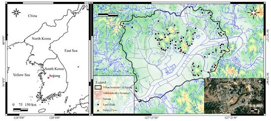
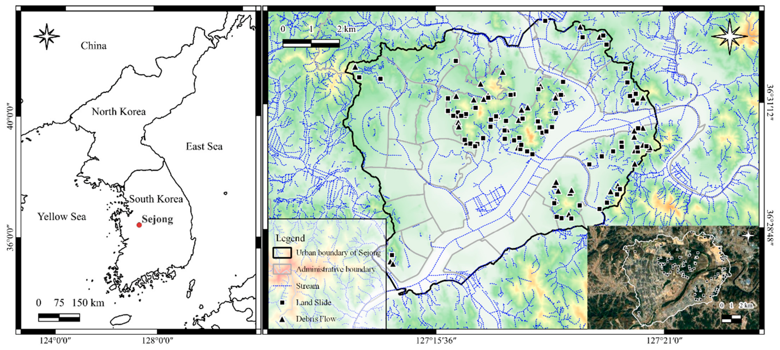
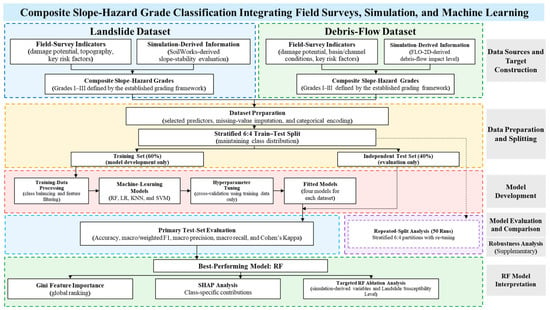
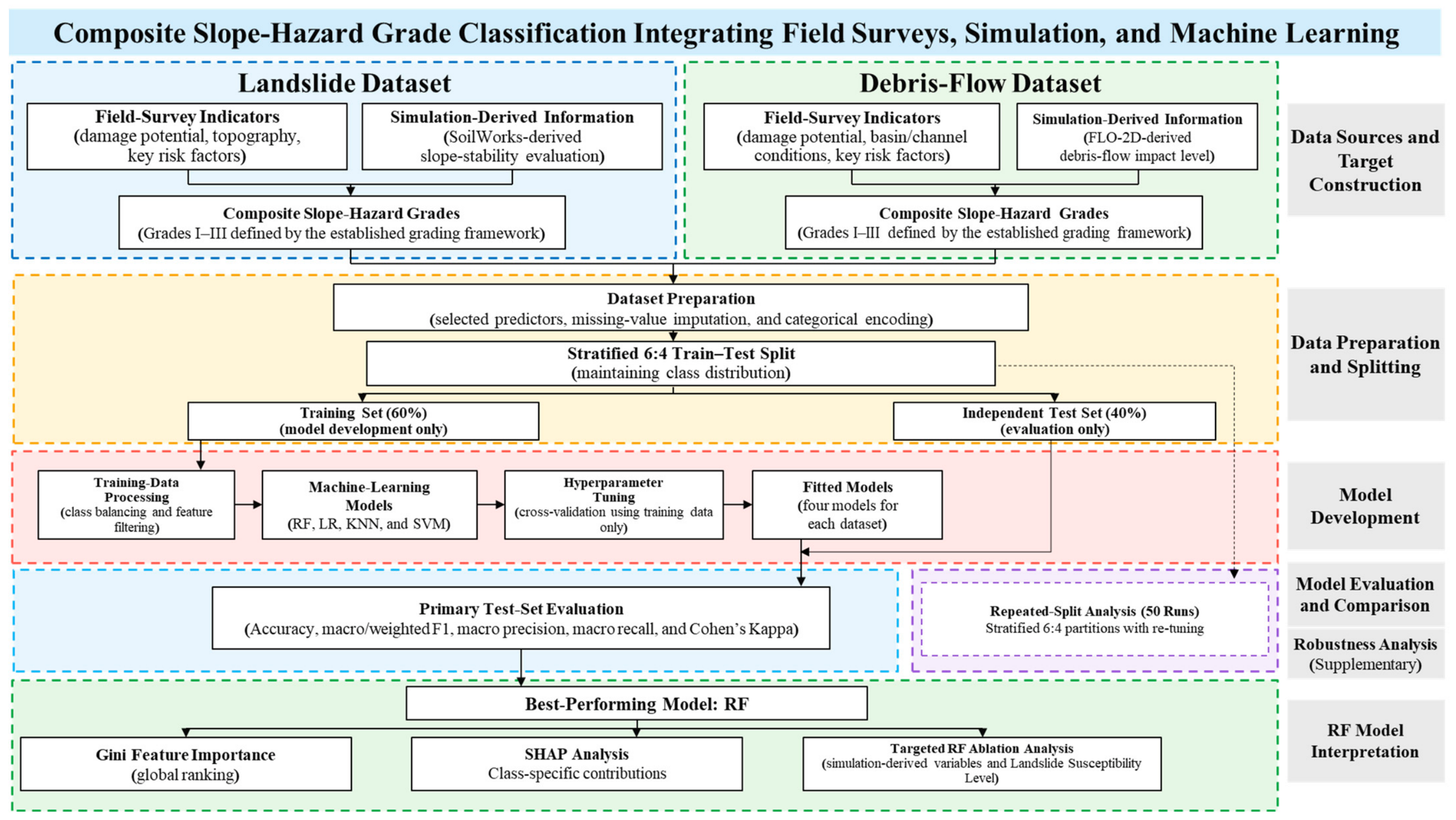
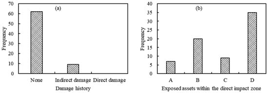
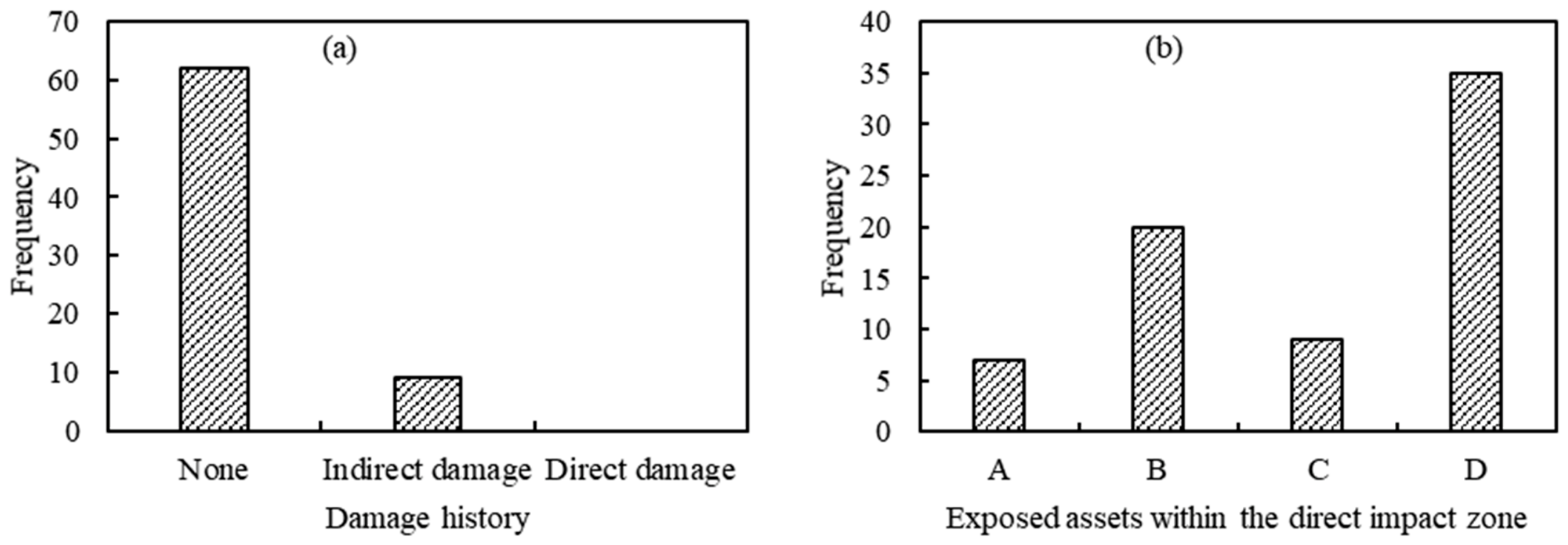
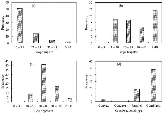
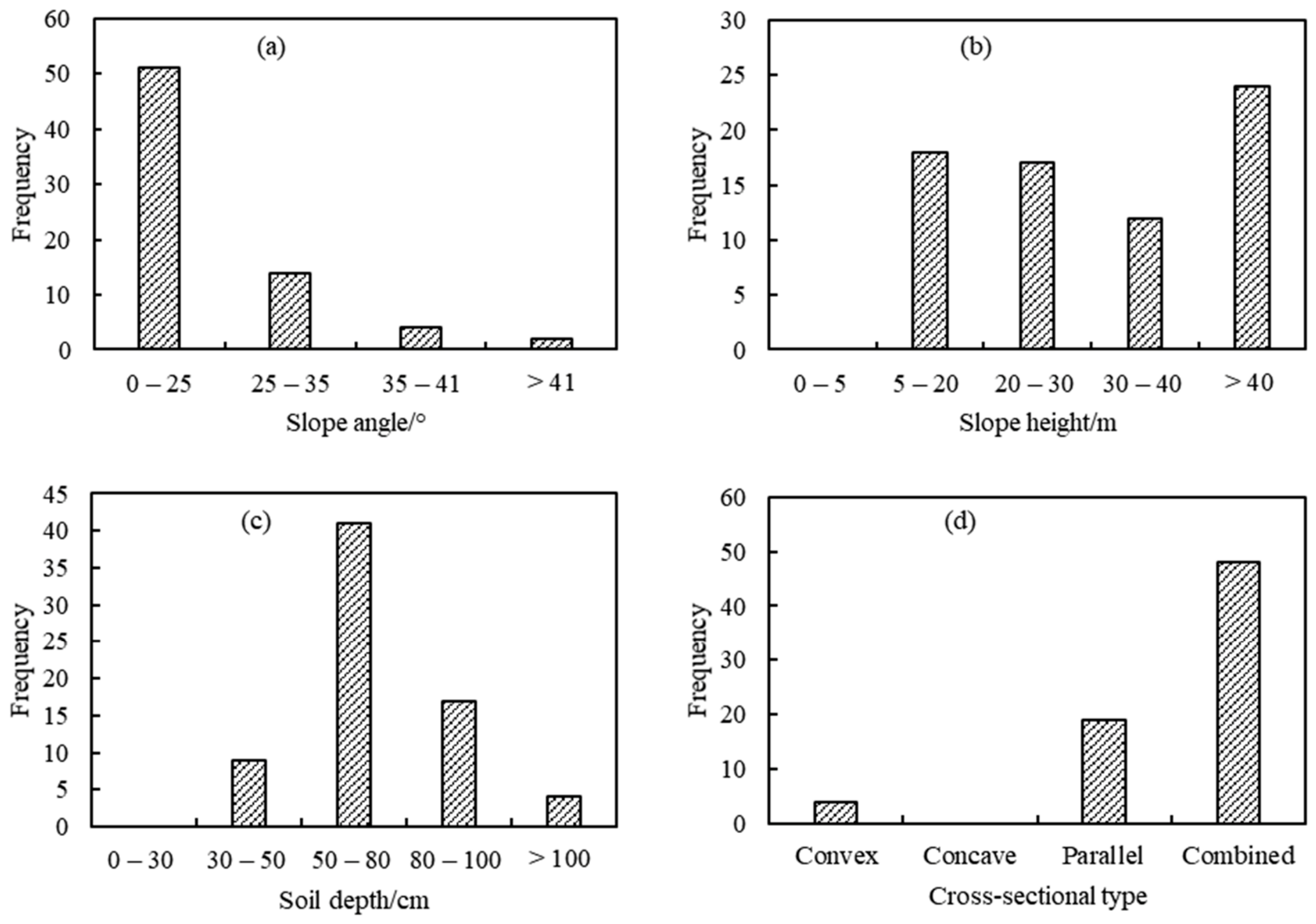
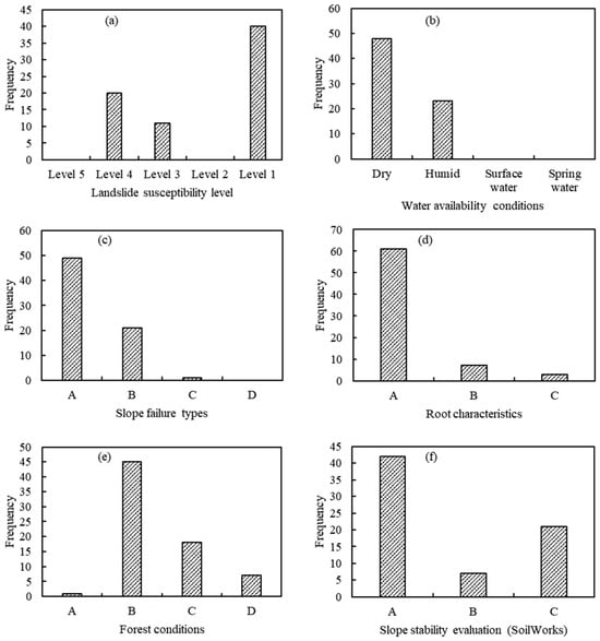
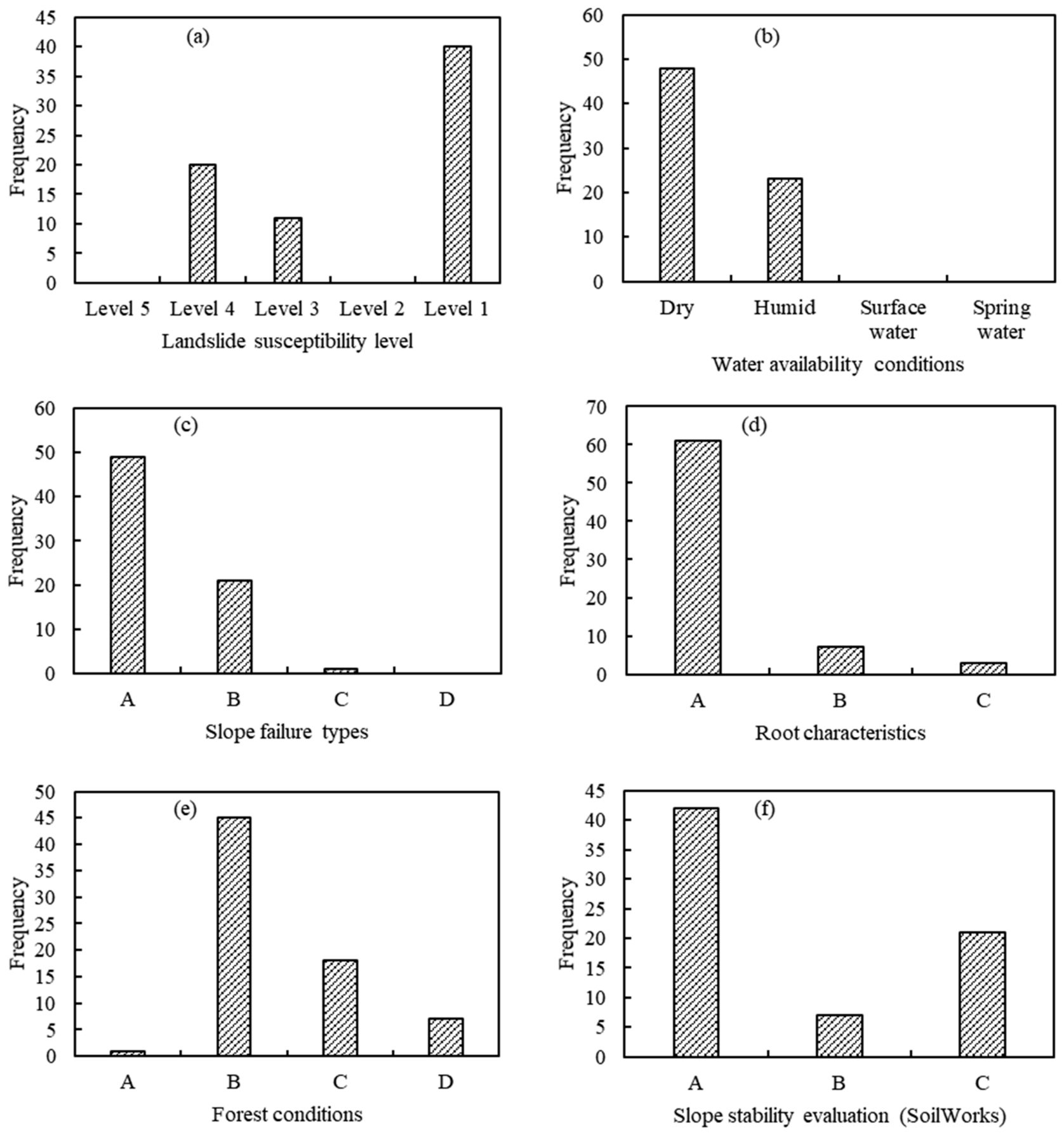
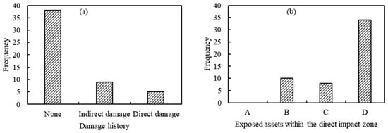
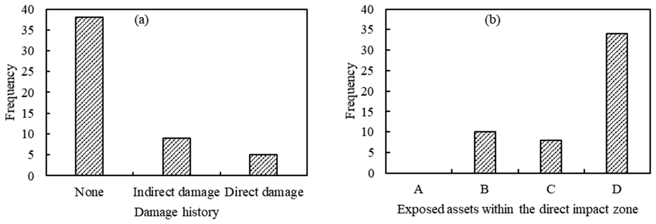
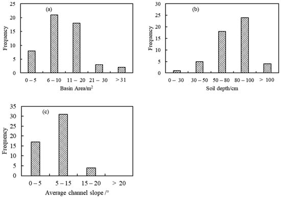
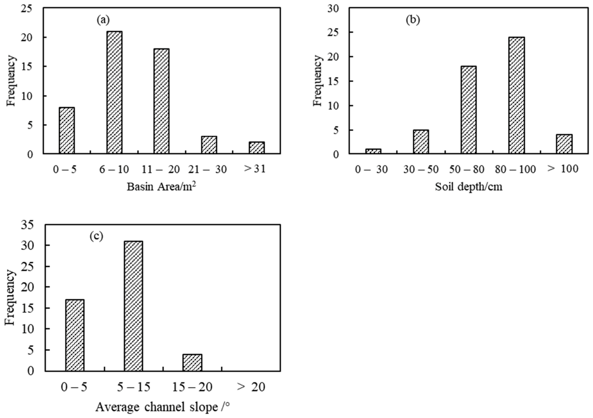
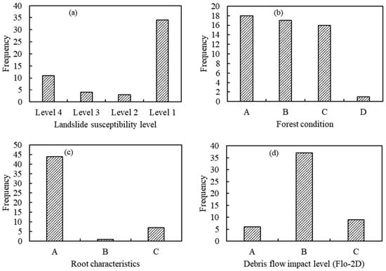
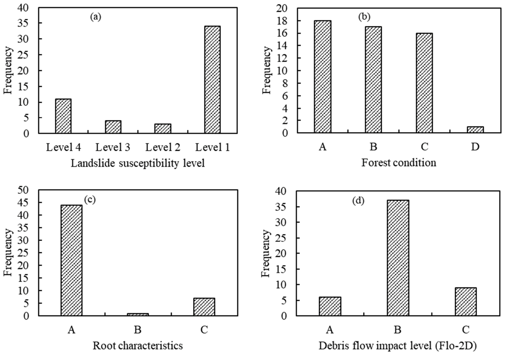
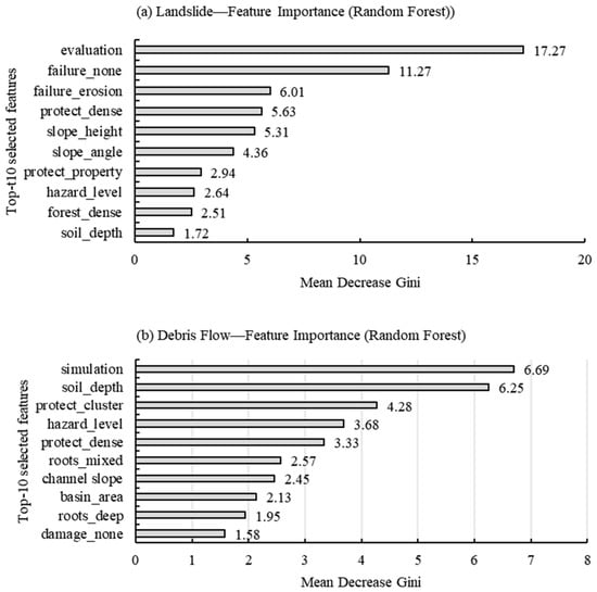
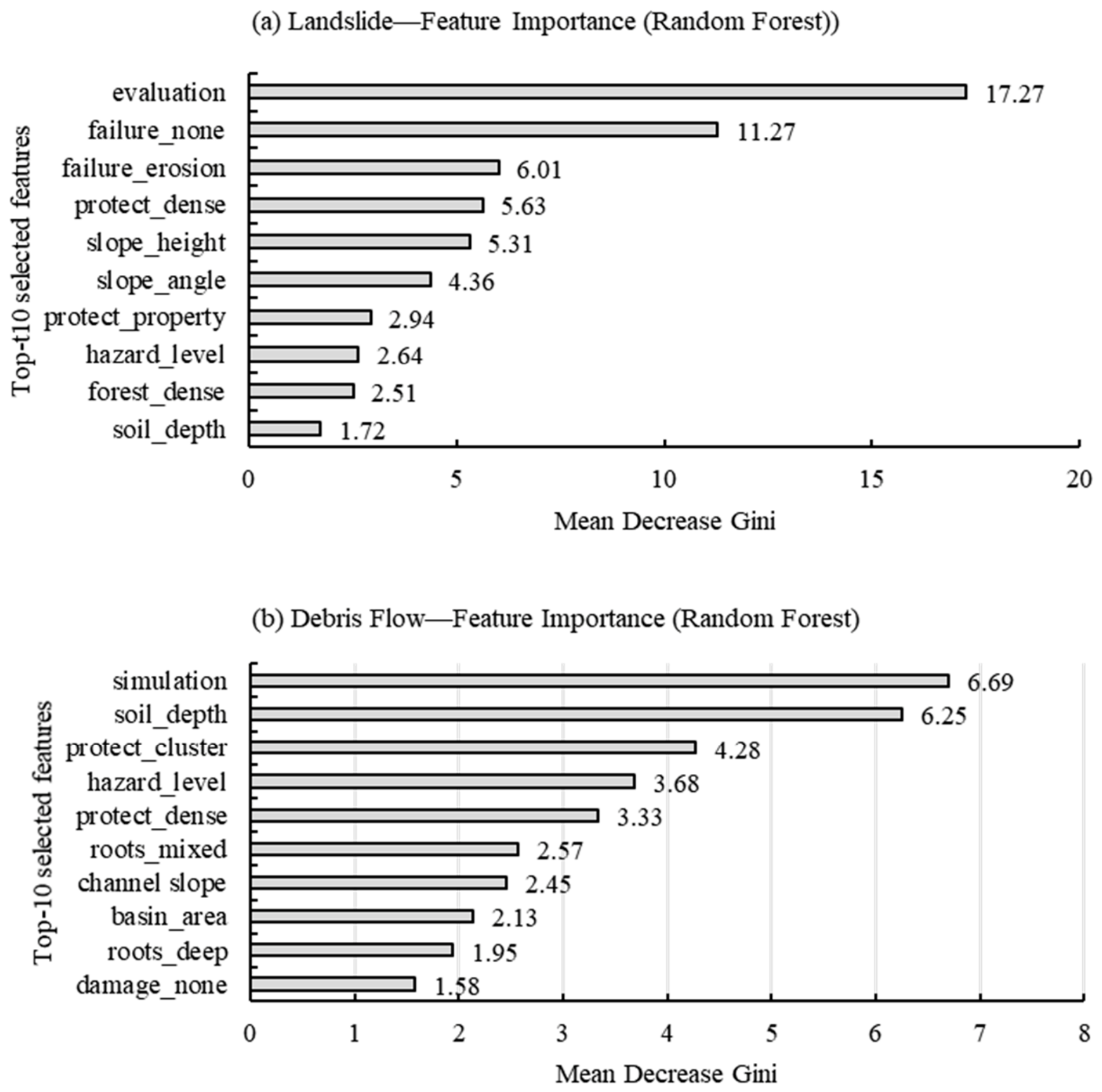
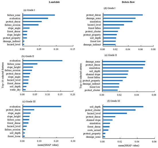
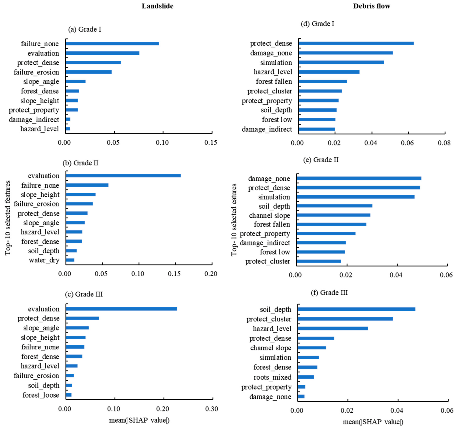

Disclaimer/Publisher’s Note: The statements, opinions and data contained in all publications are solely those of the individual author(s) and contributor(s) and not of MDPI and/or the editor(s). MDPI and/or the editor(s) disclaim responsibility for any injury to people or property resulting from any ideas, methods, instructions or products referred to in the content. |
© 2026 by the authors. Licensee MDPI, Basel, Switzerland. This article is an open access article distributed under the terms and conditions of the Creative Commons Attribution (CC BY) license.