


Abstract
Particleboard has been widely used in furniture manufacturing, architectural decoration, packaging and logistics applications, and transportation, owing to its strong raw material adaptability, relatively low cost, and favorable processing performance, making it one of the foundational materials in the wood-based panel industry. Its surface quality directly determines the added value of final products. However, in actual production environments, the complex background textures of particleboard surfaces and the low contrast between defects and the background pose substantial challenges to automatic surface defect recognition. To address these issues, this paper proposes SFNet, a particleboard surface defect recognition network integrating spatial-domain and frequency-domain feature enhancement. The network adopts EfficientNet-B0 as its backbone, introduces a Dynamic Matrixed Color Correction (DMCC)module after Block 4 to adaptively adjust feature channel weights via a dynamic temperature mechanism, thereby enhancing the feature saliency of defects in the spatial domain, and embeds a Wavelet Transform Convolution module (WTConv) after Block 6 to map spatial features into the frequency domain, leveraging the differences in frequency response between defects and the background to improve the model’s sensitivity to high-frequency defect features and multi-scale texture information. The dataset comprised 2405 high-confidence defective image patches, including 2005 patches for the main classification experiment and 400 independent patches for illumination-robustness testing. Experimental results show that SFNet was evaluated on a test set of 401-images encompassing five types of defects on particleboard surfaces, namely shavings, dust spots, oil spots, glue spots, and pollution. Across five random seeds, the model achieved an average accuracy of 97.86% ± 0.28%, with the highest single-run accuracy reaching 98.25%. It outperforms the baseline classification models used for comparison in terms of accuracy, precision, recall, and F1-score. Grad-CAM visualization results further demonstrate that SFNet can effectively suppress interference from complex background textures and accurately focus on defective regions. These results indicate that the proposed method exhibits strong robustness and recognition stability, providing an efficient and reliable solution for automated particleboard surface quality inspection in industrial scenarios.
1. Introduction
Particleboard is an engineered wood panel manufactured from wood or lignocellulosic materials (e.g., wood chips, shavings, and sawdust) through pulverization, drying, gluing, and high-temperature pressing [1]. It offers advantages such as low cost, favorable dimensional stability, good machinability, and environmental friendliness, and is therefore widely employed in furniture manufacturing and architectural decoration [2,3]. In actual production processes, due to the influence of multiple factors including raw material characteristics, adhesive application, process parameters, and production line operating conditions, the surface of particleboard is prone to various types of defects such as large shavings, dust spots, and oil stains [4]. These defects not only directly compromise product quality and degrade mechanical properties but may also damage corporate brand image and result in economic losses [5]. As one of the key categories of wood-based panels, with the continuous increase in particleboard output, establishing an efficient and reliable quality inspection system is of critical importance for ensuring product quality [6].
In earlier particleboard production, surface quality inspection relied mainly on manual operations. The process was initiated by production line operators through preliminary screening based on light reflection. Defects were then examined in detail and graded in a dedicated manual inspection area [7]. In recent years, computer vision technology has developed rapidly and has been applied across a wide range of fields [8]. Extensive research has been conducted on non-destructive inspection in the field of surface defect recognition for wood-based panels. For example, Singh et al. [9] used machine vision technology in combination with a multi-class support vector machine (SVM) classifier to detect defects in images. The proposed framework effectively classified defective images and achieved an overall classification accuracy of 99.7%. Xu et al. [10] successfully applied a frequency scanning method to detect cavity defects by investigating the natural frequency of wood. However, these methods largely depend on factors such as the mechanical equipment and image quality. Because they are highly sensitive to illumination changes and external environmental conditions, their robustness and generalization ability remain limited [11,12].
Deep learning has gradually become a mainstream approach for industrial surface defect recognition because of its robust generalization capability and powerful automatic feature extraction ability [13]. Unlike conventional methods, convolutional neural networks (CNNs) do not rely on cumbersome manual feature design but can automatically learn feature representations ranging from low-level textures to high-level semantics, thereby showing strong robustness in complex backgrounds and environments. In recent years, deep learning has been widely applied to surface defect recognition in various materials, such as steel and fabrics, and has achieved promising accuracies. For example, Li et al. [14] proposed a deep learning model based on a multi-scale feature extraction module for steel surface defect recognition and achieved state-of-the-art performance. Nasim et al. [15] used an improved YOLOv8 model to detect fabric defects in real industrial environments and ultimately obtained an accuracy of 85%. To address challenges such as the difficulty of recognizing defects in complex backgrounds, the weak semantic information of tiny defects, and the significant variations in defect targets, Chen H [16] proposed WTCF-Net for industrial surface defect detection, including defects on steel surfaces and printed circuit boards. The method incorporates a Wavelet Feature Convolution (WFC) module and an Interactive Residual Module (IRM). Compared with the baseline model, WTCF-Net improves the mAP by 5.9%, 1.3%, and 1.4% on different datasets, respectively, while achieving a detection speed of 53 FPS, demonstrating both high detection accuracy and real-time performance.
Although deep learning has achieved remarkable success in various industrial defect inspection tasks, particleboard surface defect recognition still faces unique challenges. Unlike steel or fabric surfaces, which often have relatively uniform backgrounds, particleboard surfaces contain irregular and highly heterogeneous wood-chip textures. These complex background textures may interfere with the extraction of subtle defect features by neural networks, resulting in missed detections and false alarms [4]. To address this problem, researchers have proposed various improved models in recent years. For example, Wang et al. [17] developed an improved YOLOv5s model by introducing a coordinate attention mechanism and a spatial pyramid pooling-fast (SPPF) module, which effectively enhanced the recognition of blurred defects on particleboard surfaces and achieved an mAP of over 90%. Zhang et al. [18] proposed a dual-attention module, DC-DACB, which combined an anomaly detection network with a residual network to improve defect feature representation and achieved a recognition success rate of 93.1% under blurred background conditions. Li et al. [19] integrated multiple improvement strategies and increased the precision of particleboard surface defect recognition by 9.4% compared with R-CNN.
The above studies have improved the detection accuracy of particleboard surface defects to some extent by introducing attention mechanisms or optimizing backbone networks. However, significant challenges remain in practical industrial inspection. Although ResNet-based models or complex two-stage networks can extract rich feature representations, their high computational cost makes it difficult to achieve high-speed online inspection on edge-embedded devices with limited computing resources, preventing them from meeting the stringent real-time requirements of production lines [20,21]. In addition, most existing improvement strategies are limited to feature enhancement in the spatial domain [22]. In terms of spatial pixel distribution, particleboard surface textures are highly similar to subtle defects, such as small shavings, dust spots, and tiny oil spots. Therefore, conventional convolutional neural networks that rely solely on spatial features often struggle to effectively decouple strong background noise from weak defect signals, resulting in a relatively high missed-detection rate under complex texture interference.
To overcome these limitations, this study proposes a novel particleboard surface defect recognition network, termed SFNet. The network adopts EfficientNet-B0 as the backbone and models subtle surface defect features from both spatial and frequency domains. To address illumination fluctuations and the low contrast between defects and the background in particleboard production environments, a Dynamic Matrixed Color Correction module, DMCC, is designed. This module captures global statistical information through a dynamic temperature mechanism and adaptively reweights feature channels using matrix transformation. As a result, DMCC helps alleviate the influence of unstable imaging quality during feature extraction and enhances the saliency of weak defects, such as oil spots and dust spots. After spatial feature enhancement, a Wavelet Transform Convolution module, WTConv, is introduced to further extract frequency-domain texture features. WTConv was designed to overcome the bottleneck of spatial-domain analysis. It innovatively transformed features into the frequency domain for processing and effectively suppressed background texture noise by exploiting the intrinsic differences in the frequency response between defects and the wood-grain background. Through dual-domain enhancement in the spatial and frequency domains, precise recognition of tiny defects under complex particleboard texture backgrounds was achieved.
2. Materials and Methods
2.1. System Design
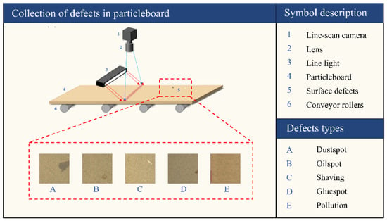
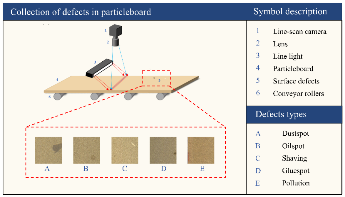
In this study, a dataset was constructed based on an actual production line at Jiangsu Suqian Daya Wood Industry Co., Ltd. (Suqian, China). The experimental material was multilayer homogeneous eco-friendly particleboard with dimensions of 1220 mm × 2440 mm. During image acquisition, a line-scan camera scanned the particleboard surface line by line through a lens, while the board was being conveyed. Each exposure captured a line of scan data along the board width direction. The specific parameters of the camera, lens, light source, and light source controller are presented in Table 1 below. As the particleboard moved along the conveying direction, line data from different positions were sequentially stitched in temporal order to form a complete two-dimensional surface image. The final images contained five typical defect categories: Shaving, Dustspot, Oilspot, Gluespot, and Pollution, the first four categories represent specific defect types with distinct visual characteristics, while Pollution serves as a catch-all category designed to accommodate extraneous contamination that cannot be classified into the aforementioned four categories. The overall particleboard defect recognition system is shown in Figure 1.
Table 1.
Device Parameters.
Figure 1.
Particleboard defect recognition system.
2.2. Dataset Construction
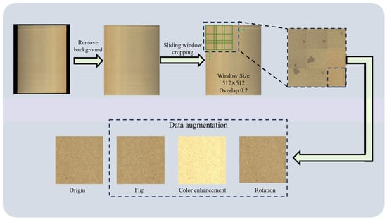
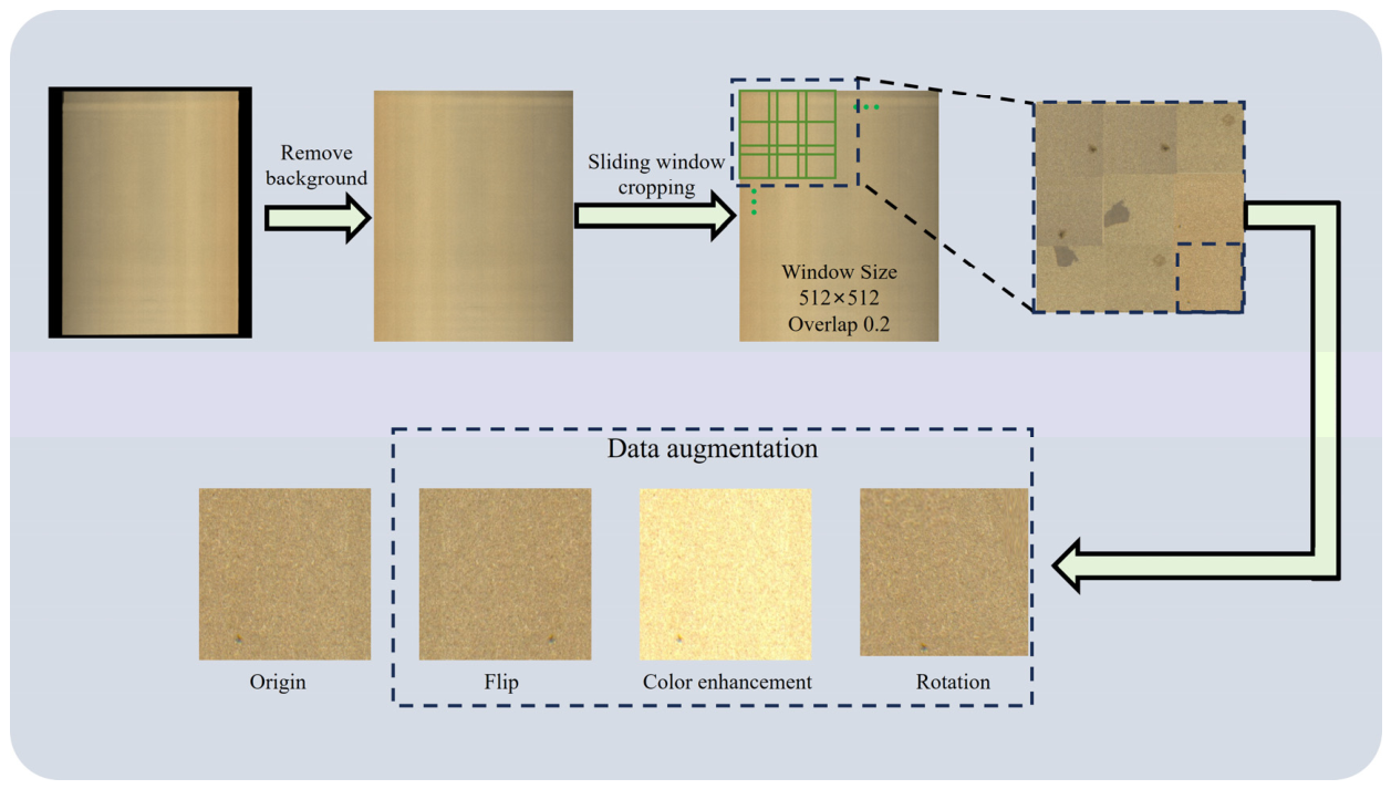
This study collected 487 original full-size particleboard surface images from Jiangsu Dare Wood Industry Co., Ltd (Danyang, Jiangsu, China), including 280 images acquired under 240 lux illumination and 207 images acquired under 160 lux illumination. Each original image had a resolution of approximately 7000 × 15,500 pixels. To satisfy the input-size requirement of the defect-recognition model, the original images were cropped using a 512 × 512 sliding window with a 20% overlap. Additional cropping windows were retained at the image edges to avoid the loss of edge-defect information. Using this strategy, each full-size image generated 646 candidate sub-images, resulting in a total of 314,602 candidate sub-images from the 487 original images, as illustrated in Figure 2.
Figure 2.
Defect processing workflow.
To prevent data leakage, the dataset was partitioned at the original full-size image level before cropping and data augmentation. All sub-images derived from the same original image were assigned to the same subset, ensuring that sub-images originating from the same board image were not split between the training and test sets. Data augmentation was applied only to the training subset after this source-level partitioning.
Since only a small proportion of the cropped candidate sub-images contained identifiable defects, a rigorous manual screening process was conducted by experienced inspectors. Only images with clear defect morphology and unambiguous category labels were retained, yielding 2405 high-confidence defective images. Among them, 2005 images were used as the primary classification dataset, including 1020 images acquired under 160 lux and 985 images acquired under 240 lux. After source-level partitioning, this dataset was divided into 1604 training images and 401 primary test images. The remaining 400 images were reserved as an independent illumination-robustness test set, consisting of 200 images acquired under 160 lux and 200 images acquired under 240 lux. These 400 images were not used for model training or model selection and were used exclusively to evaluate the robustness of the DMCC module under different illumination conditions.
All retained images belong to one of five defect categories: Shaving, Dustspot, Oilspot, Gluespot, and Pollution. The number of images in each category and their distribution across illumination conditions are reported in Table 2.
Table 2.
Dataset size.
Data augmentation was performed exclusively on the training set to increase sample diversity. The augmentation operations included image flipping, color augmentation, and rotation, expanding the training set from 1604 to 6416 images. No augmentation was applied to either the primary test set or the independent illumination-robustness test set. During training, images acquired under 160 lux and 240 lux were mixed, enabling the model to learn defect representations under different illumination conditions.
2.3. SFNet Architecture
2.3.1. Overall Framework
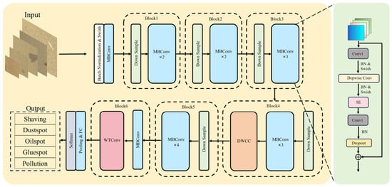
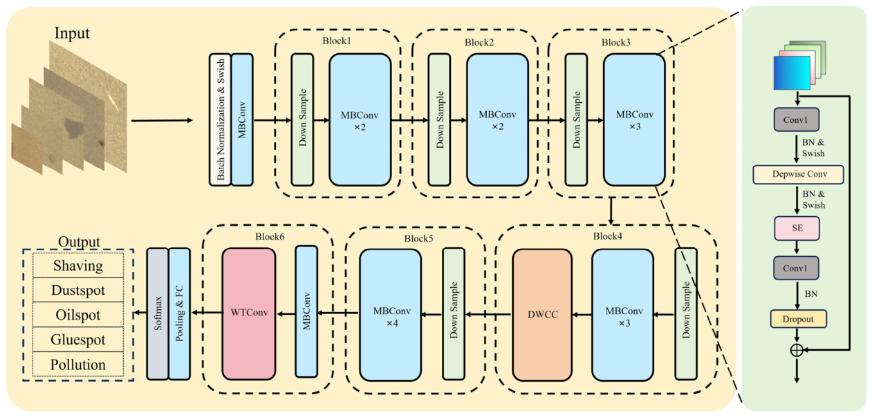
The architecture of SFNet (Spatial-Frequency EfficientNet) is shown in Figure 3. SFNet uses EfficientNet as the backbone, into which the DMCC and WTConv modules are inserted, thereby integrating a dual-feature enhancement mechanism in the spatial and frequency domains. After a series of convolutional operations, the final classification results are obtained. The basic convolutional block is the MBConv block, which consists of six key components: a 1 × 1 expansion convolution, a Batch Normalization layer, the Swish activation function, depthwise convolution, an SE (Squeeze-and-Excitation) attention module, and a residual connection. The particleboard images acquired by the industrial camera were preprocessed and resized into 224 ×224 image patches before being fed into the convolutional neural network. The 1 × 1 convolution first expanded the input features to increase the number of feature channels and optimize the computational process. Depthwise convolution efficiently extracts the spatial features of an image while reducing the number of parameters. Batch Normalization normalizes batch features, accelerates network training, and alleviates internal covariate shifts, thereby improving training stability and accuracy. The Swish activation function replaces the conventional ReLU function and introduces smooth non-monotonicity, which improves the gradient flow in deep networks. The SE module explicitly models inter-channel dependencies and adaptively recalibrates channel-wise feature responses, thereby enhancing the network sensitivity to important features [23].
Figure 3.
Architecture of SFNet.
To address the difficulty of distinguishing particleboard surface defects from background textures owing to their high similarity, a dual-domain fusion strategy was introduced into the conventional CNN framework. First, a DMCC module was embedded after Block 4. This module incorporates a lightweight dynamic temperature parameter adjustment mechanism that adaptively aggregates global contextual information and helps the network rapidly locate tiny defective regions under complex wood-chip backgrounds. Second, a Wavelet Transform Convolution (WTConv) module was embedded after Block 6. This module uses wavelet transform to extract multi-scale texture features in the frequency domain, thereby enhancing the model’s ability to perceive subtle texture variations on particleboard surfaces and effectively reducing the interference of background noise in foreign-object recognition. Finally, the enhanced feature maps were passed through global average pooling and a fully connected layer, and the Softmax function was used to achieve precise classification of five defect categories: Shaving, Dustspot, Oilspot, Gluespot, and Pollution.
2.3.2. DMCC Module
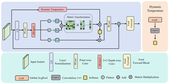
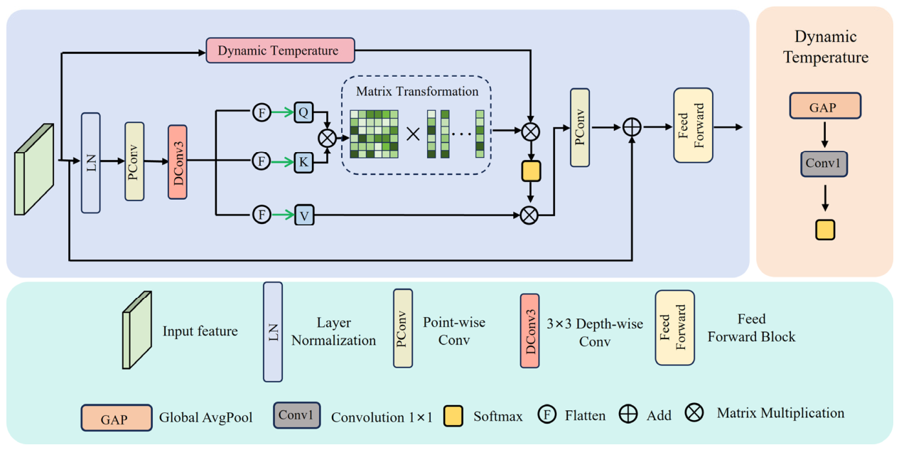
In the task of particleboard surface defect recognition, the image background is composed of irregular wood-chip textures, whereas common defects such as oil stains and glue spots are typically characterized by small size and low contrast against the background. When dealing with such high-frequency textured backgrounds, conventional CNNs are easily disturbed by background noise and therefore struggle to accurately localize weak defect features. Matrix transformation is commonly used in standard ISP pipelines to process global color and illumination information, and it can also enhance and refine local image details [23]. Based on this principle, the Dynamic Matrixed Color Correction Block (DMCC) was introduced to suppress background textures and enhance defect features by exploiting its global receptive field [24]. The DMCC module mainly consists of three key steps: multi-scale feature projection, dynamic temperature estimation, and weighted matrix transformation. The architecture of the DMCC module is shown in Figure 4.
Figure 4.
Architecture of the DMCC module.
For a given input feature map normalization was first performed. A projection strategy was adopted to simultaneously capture the semantic dependencies across channels and local spatial context. Specifically, the features were first projected into a latent space using a point wise convolution, followed by a depth wise convolution and a flattening operation. After flattening, preliminary Query (Q), Key (K), and Value (V) mappings were generated. A transformation matrix was then obtained through matrix multiplication. This process can be expressed as:
Illumination fluctuations in industrial production environments, together with color variations among different particleboard batches, cause the contrast between defects and the background to vary. To address defects that are difficult to distinguish, a dynamic temperature mechanism was designed to generate a scaling factor adaptively according to the global statistical information of the input feature map. Specifically, global statistical information was first aggregated using global average pooling, and a dynamic temperature τ was then generated through a nonlinear transformation layer. This process can be expressed as:
where σ denotes the Softmax function, and α and β are predefined scaling and bias parameters, respectively. This operation enables the region of interest to be adaptively adjusted according to the complexity of the image content. Using the generated Q, K, and dynamic temperature τ, the inter-channel correlation matrix M can be calculated. The dynamic temperature τ is injected before the Softmax operation to assign attention scores to different regions:
Finally, M was used to linearly transform V, and the result was fused with the residual connection and feed forward network (FFN) to obtain the final output Y:
The DMCC module implements a complete process from global texture suppression to local defect enhancement, thereby effectively improving the defect recognition performance.
2.3.3. WTConv Module
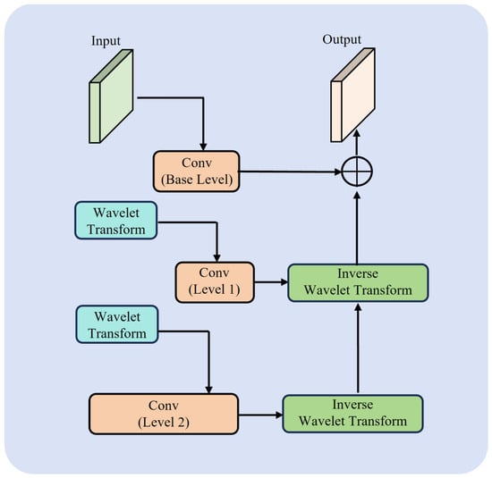
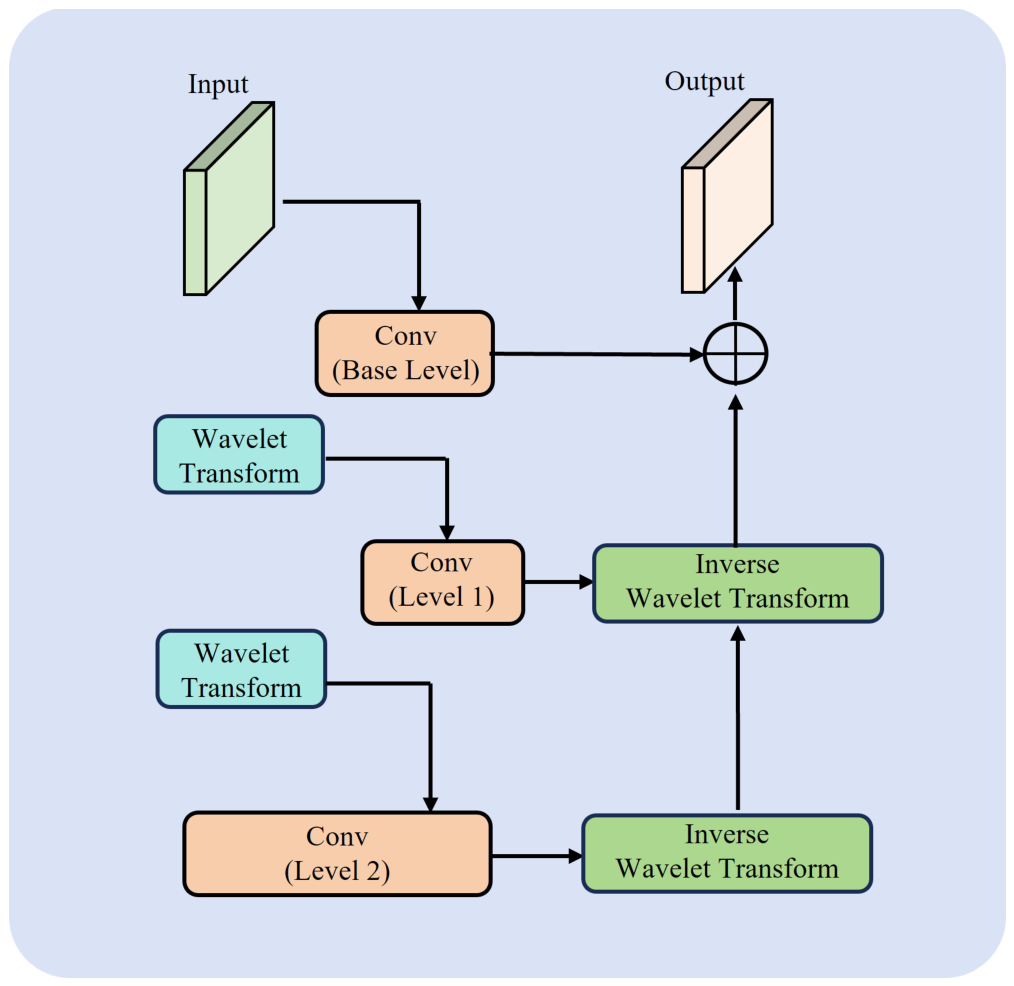
After the defect feature saliency was enhanced by the DMCC, the discriminability between particleboard surface defects and the background textures increased. However, conventional CNNs still struggle to separate high-frequency defect details from complex background textures. Although defects and the backgrounds are difficult to distinguish in the spatial domain at the pixel level, they often exhibit different energy distributions in the frequency domain. Background wood-chip textures typically appear as uniformly distributed high-frequency noise, whereas defect regions correspond to abrupt changes within specific frequency bands. Inspired by this observation, the WTConv module was introduced to exploit the multi-scale time–frequency analysis capability of wavelet transform and enhance the model’s perception of multi-scale texture details from the frequency domain perspective. The architecture of the WTConv is shown in Figure 5 [25,26].
Figure 5.
Architecture of the WTConv module.
First, for a given input tensor , discrete wavelet transform (DWT) was used to decompose it into four sub-bands: the low-frequency component XLL, and the high-frequency components in the horizontal, vertical, and diagonal directions, namely XLH, XHL and XHH. To effectively extract features in the frequency domain, depthwise convolution was applied to these frequency components, and the output was reconstructed through inverse wavelet transform (IWT). The single-level process can be formalized as:
where WT(X) denotes the transformation of the input X into a frequency-domain tensor containing XLL, XLH, XHL and XHH; W represents the depthwise convolution kernel weights, with an input channel number of 4C. This operation not only enables the independent enhancement of frequency-domain features but also allows a small convolution kernel to achieve a larger receptive field on the down sampled frequency-domain maps relative to the original input.
To capture multi-scale defect features, the above process was extended to a multi-level cascaded structure. In the i-th decomposition stage, the low-frequency component XLL(i−1) from the previous stage was further decomposed by wavelet transform, while the high-frequency components were directly involved in convolutional processing. The decomposition and convolution processes at the i-th stage are defined as:
where XH(i) denotes the collection of all three high-frequency components at the i-th stage, namely XLH(i), XHL(i) and XHH(i).
To fuse frequency-domain features at different scales, the linear superposition property of wavelet transform was utilized, and the outputs were aggregated through progressive reconstruction. The aggregated output Z(i) at the i-th stage was reconstructed jointly from the low-frequency convolution result of the current stage and the aggregated result of the next stage as follows:
where Z(i−1) represents the multi-scale frequency-domain features aggregated from the (i − 1)-th stage. The final module output Xout combines the spatial features of the original input with the multi-scale frequency-domain features, and is expressed as:
This design ensures that the model can preserve the macroscopic structural information of the particleboard while markedly enhancing its perception of the high-frequency textures of tiny defects, thereby significantly improving the classification accuracy.
2.4. Experimental Environment
The hardware and software configurations used in this study are presented in Table 3.
Table 3.
Hardware and software configurations.
2.5. Evaluation Metrics
To compare the performances of different models in particleboard surface defect recognition, a series of evaluation metrics was introduced. In this study, the classification performance was evaluated using four metrics: accuracy (), recall (), F1-score (), and precision (). These metrics were used to effectively assess the performance of the classification models. The specific formulas are as follows:
where TP denotes true positives, namely the number of samples that actually belong to the positive class and are correctly predicted as positive; TN denotes true negatives, namely the number of samples that actually belong to the negative class and are correctly predicted as negative; FP denotes false positives, namely the number of samples that actually belong to the negative class but are incorrectly predicted as positive; and FN denotes false negatives, namely the number of samples that actually belong to the positive class but are incorrectly predicted as negative. represents the overall proportion of correctly classified samples. indicates the proportion of samples predicted as positive that are actually positive. is the harmonic mean of precision and recall and can be used to comprehensively evaluate the model’s ability to identify the positive class. measures the model’s ability to capture positive samples, that is, the proportion of actual positive samples that are correctly classified as positive. Taken together, these four performance metrics provide a scientific and effective evaluation of the accuracy of the proposed model.
3. Experiments and Analysis
3.1. Hyperparameter Settings
In practical model training, hyperparameters are critical to model performance [27]. The hyperparameter settings used in this study are presented in Table 4.
Table 4.
Hyperparameter configuration results.
3.2. Experimental Results of SFNet
To assess the influence of stochastic factors, including random weight initialization and data shuffling, five independent training trials were conducted using random seeds 0, 1, 2, 3, and 4. The same training set, test set, network architecture, hyperparameters, training strategy, and evaluation protocol were used in all trials. Each model was trained for a fixed 200 epochs, and the final checkpoint from each trial was evaluated once on the untouched test set after training.
As summarized in Table 5, SFNet achieved test accuracies ranging from 97.51% to 98.25%, with a mean accuracy of 97.86% ± 0.28%. The mean precision, recall, and F1-score values were 98.02% ± 0.44%, 98.15% ± 0.21%, and 97.88% ± 0.42%, respectively. The relatively small standard deviations indicate that SFNet is not highly sensitive to random initialization or training-data shuffling, demonstrating good training stability and reproducibility.
Table 5.
Performance stability of SFNet across five independent training trials with distinct random seeds.
3.3. Test of the Superiority of EfficientNet
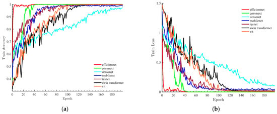
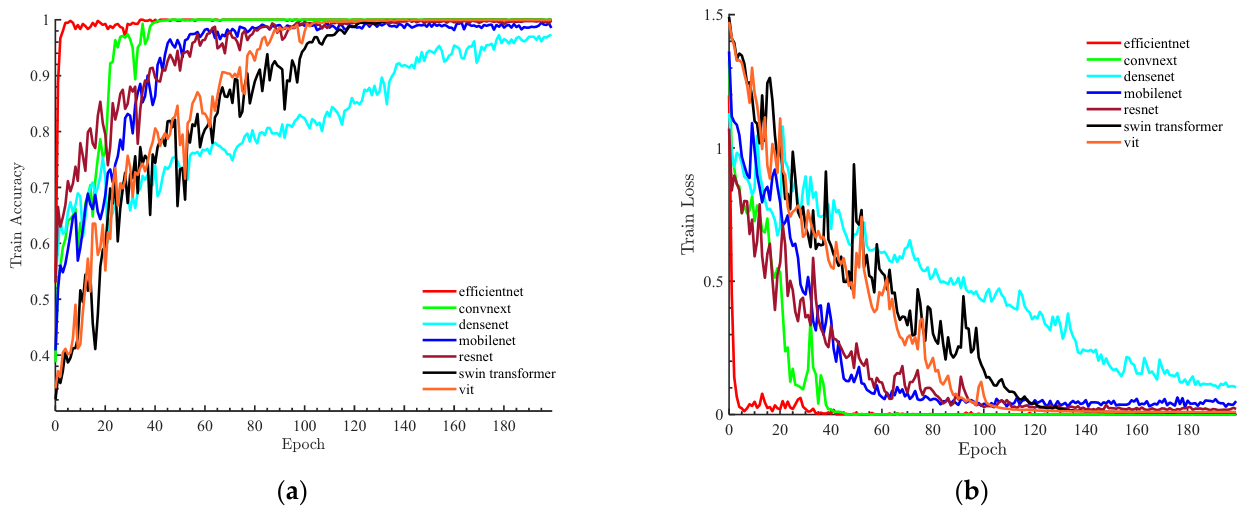
To verify the superiority of EfficientNet-B0 as the baseline model for further improvement, six classical neural networks, namely ConvNeXt [28], DenseNet [29], MobileNetV2 [30], ResNet50 [31], Swin Transformer [32], and Vision Transformer (ViT) [33], were compared with EfficientNet. All comparative models were trained and evaluated under strictly identical experimental conditions—including dataset partitioning, input resolution (224 × 224), cross-entropy loss function, Adam optimizer (with fixed learning rate and weight decay), batch size of 64, total training epochs (200), and evaluation metrics—to ensure methodologically sound and directly comparable performance assessment. The training dynamics, including accuracy progression and loss evolution, are illustrated in Figure 6. Table 6 presents a comprehensive comparison of final test performance against model complexity, quantified by parameter count (Params) and computational cost (FLOPs).
Figure 6.
Training accuracy and training loss curves of the seven classification models. (a) Training accuracy of the models. (b) Training loss.
Table 6.
Comparison of performance and computational complexity among seven basic classification models.
Figure 6a,b depicts the training accuracy and training loss curves of the seven comparative models. EfficientNet-B0 exhibits rapid initial convergence, characterized by a steep increase in training accuracy and an overall decline in training loss. In contrast, MobileNetV2, despite its computational efficiency with 2.2303 M parameters and 0.3262 GFLOPs, shows limited representational capacity for extracting fine-grained surface textures and low-contrast defect features. Swin Transformer and Vision Transformer employ self-attention mechanisms to capture long-range dependencies and global contextual information. However, their performance under the present experimental conditions may be constrained by the limited dataset size and sensitivity to optimization settings. ConvNeXt-Tiny and ResNet50 provide robust local feature representations but converge more slowly and achieve lower final performance than EfficientNet-B0. DenseNet121 benefits from dense connections and hierarchical feature reuse; however, its feature-reuse mechanism may also retain redundant background texture information, which could reduce its discriminative effectiveness for this dataset.
The final test-set results are reported in Table 6. EfficientNet-B0 achieves the highest test accuracy of 94.51%, with precision, recall, and F1-score values of 94.06%, 94.27%, and 94.15%, respectively. Its accuracy surpasses that of DenseNet121, the second-best-performing model, by 3.24 percentage points and exceeds that of Swin Transformer by 3.49 percentage points. In addition, EfficientNet-B0 contains only 4.0140 M parameters and requires 0.4139 GFLOPs, demonstrating a favorable balance between classification performance and computational cost.
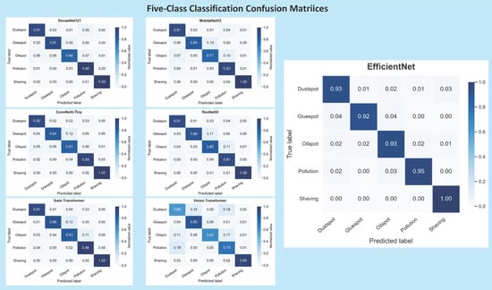
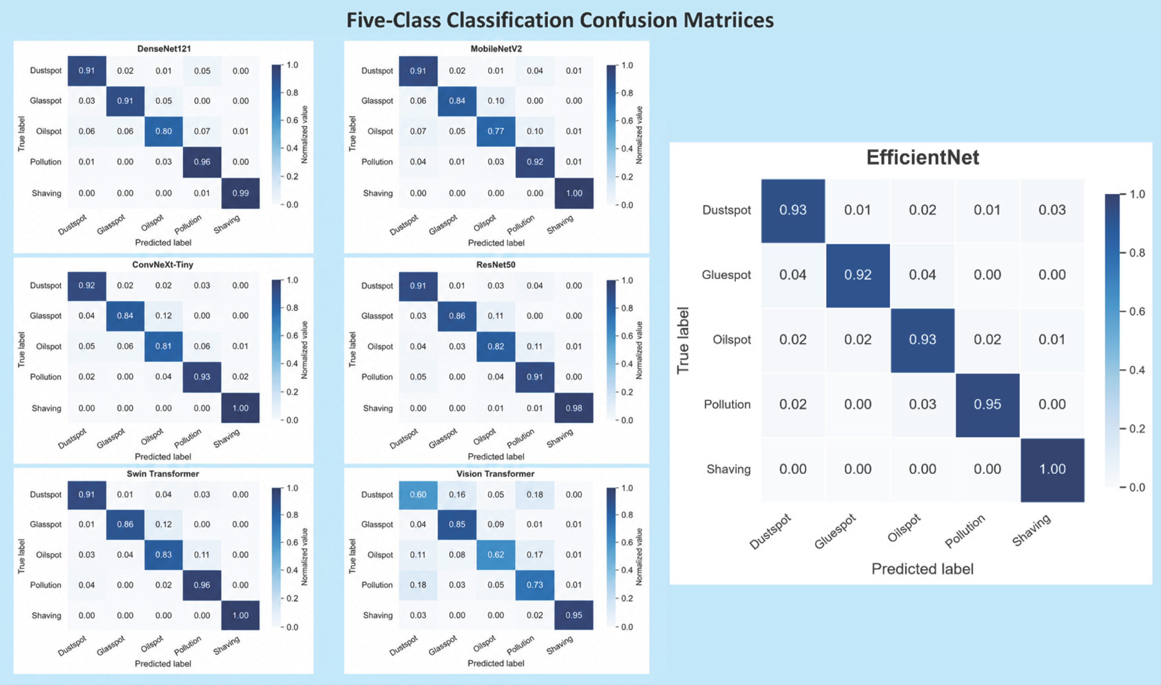
Figure 7 presents the normalized confusion matrices of the seven baseline models across the five defect categories. EfficientNet-B0 shows a predominantly diagonal prediction pattern, indicating relatively high recognition performance across the defect classes and fewer off-diagonal misclassifications. In comparison, the other models exhibit more pronounced inter-class confusion, particularly between categories with similar surface textures or subtle morphological differences. These observations are consistent with the quantitative results in Table 6, where EfficientNet-B0 achieves the highest accuracy, precision, recall, and F1-score. The results indicate that EfficientNet-B0 provides stronger discriminative capability for fine-grained particleboard defect classification.
Figure 7.
Confusion matrices of the baseline models.
Overall, EfficientNet-B0 achieves a favorable balance among convergence efficiency, classification performance, class discrimination, and computational complexity. Therefore, EfficientNet-B0 was selected as the baseline network for the subsequent integration of the DMCC and WTConv modules to construct the proposed SFNet.
3.4. Ablation Study of SFNet
To verify the effectiveness of the proposed improvement strategies, this paper conducts ablation experiments on SFNet under strictly identical experimental conditions, with the results presented in Table 7. Table 7 reports only a single independent experimental result obtained with a random seed of 2, which corresponds to the highest accuracy achieved by the complete model across five experimental runs. All baseline models and module-integrated models employ identical data partitioning, training parameters, and test sets to ensure the fairness and comparability of the comparative results.
Table 7.
Ablation study of SFNet.
Without the incorporation of DMCC and WTConv, using EfficientNet-B0 alone as the backbone network yields a model accuracy of 94.51%. Upon the addition of DMCC, the accuracy improves to 97.01%, with precision, recall, and F1-score reaching 96.84%, 97.00%, and 96.91%, respectively, indicating that DMCC can enhance the model’s capacity for modeling defect regions and their global features.
When WTConv is incorporated into EfficientNet-B0 independently, the model accuracy reaches 96.76% with a precision of 96.89%, demonstrating that WTConv can leverage frequency-domain features and multi-scale information to improve the representation of defect textures. When DMCC and WTConv are introduced simultaneously, the model achieves optimal results, with an accuracy of 98.25%, and recall and F1-score of 98.19% and 98.14%, respectively. Compared with the baseline model, the accuracy is improved by 3.74 percentage points. These results indicate that the role of DMCC in feature re-weighting and global information modeling is complementary to that of WTConv in frequency-domain feature extraction and noise suppression, and their combination can further enhance the model’s capability to identify surface defects in particleboard.
3.5. Determination of Module Placement
To explore the effect of module placement, five pre-defined configurations were compared, as shown in Table 8. It should be noted that no separate validation set was used in this study. Therefore, the same held-out test set was used both for comparing the five module-placement configurations and for reporting the final model performance. Consequently, the test set cannot be considered fully independent of the configuration selection process. The comparison in Table 8 should therefore be interpreted as an exploratory evaluation of different placement strategies rather than as definitive validation of a globally optimal configuration.
Table 8.
Comparison of the effects of module placement.
As the insertion positions of the modules progressively moved from shallow to deeper layers, the recognition metrics generally improved. Model A showed the lowest performance, suggesting that introducing complex feature calibration and frequency-domain transformation modules at very shallow layers may interfere with the extraction of basic low-level texture features. In contrast, configurations B and C achieved substantially better results, indicating that intermediate-level features may provide more suitable representations for defect enhancement.
Among the five pre-defined configurations evaluated in this study, Model D, in which the DMCC module was placed after Block 4 and the WTConv module after Block 6, achieved the highest test performance, with an accuracy, recall, F1-score, and precision of 98.25%, 98.19%, 98.14%, and 98.26%, respectively. However, because no independent validation set was used for configuration selection, this result should be interpreted as showing that Model D was the best-performing configuration under the current experimental protocol, rather than as conclusive evidence of a universally optimal module placement.
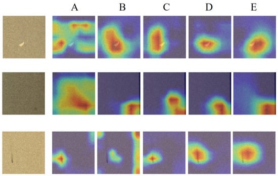
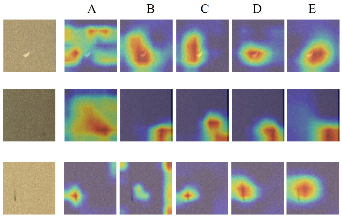
To visualize the results, Grad-CAM was used to generate heatmaps for the five models. The final heatmap comparisons are shown in Figure 8. Compared with Models A, B, C, and E, Model D was more effective at suppressing the interference from the complex background texture of particleboard and more precisely focused on the defects themselves. In particular, for the shaving defect in the first row, the heatmaps of Models A, B, and C were relatively diffuse, with large attention regions, whereas the red activation region of Model D tightly covered the main defect area. For the oil-spot defect in the second row, Model A showed an attention shift and incorrectly focused on a defect-free region, while the attention region of Model C shifted upward and was therefore less accurate. In contrast, Model D precisely localized the center of the spot. For the third type of defect, none of the models except D could completely and accurately focus on the entire curved defect, whereas Model D was still able to follow the scratch trajectory.
Figure 8.
Comparison of heatmaps for different module placements.
In summary, based on both the heatmap activation regions and the quantitative comparison of the five models, placing the DMCC module after Block 4 and the WTConv module after Block 6 enabled the most effective integration of shallow- and deep-layer semantic information, thereby maximizing recognition accuracy.
3.6. Robustness Experiments Under Different Illumination Conditions
To verify the impact of the DMCC module on model stability under different illumination conditions, the EfficientNet-B0 backbone network, WTConv module, training data, training strategy, and evaluation protocol were kept identical for both models, with the presence or absence of the DMCC module being the only experimental variable. An independent illumination-robustness test set containing 400 image patches was then divided into two subsets according to the acquisition illumination: 200 images acquired under 160 lux and 200 images acquired under 240 lux. Since both models were evaluated on the same independent illumination-robustness test subsets, the observed performance differences can be primarily attributed to the effect of DMCC on the models’ adaptability to illumination variations.
As shown in Table 9, SFNet with DMCC achieved accuracies of 98.50% and 98.00% under 160 lux and 240 lux, respectively. Since the two subsets contained equal numbers of images, the overall accuracy across the illumination-robustness test set was 98.25%, with an accuracy difference of 0.50 percentage points between the two illumination conditions. In comparison, EfficientNet-B0 + WTConv without DMCC achieved accuracies of 97.50% and 95.50%, respectively, corresponding to an overall accuracy of 96.50% and an accuracy difference of 2.00 percentage points. Adding DMCC therefore increased the overall accuracy by 1.75 percentage points and reduced the difference between the two illumination conditions by 1.50 percentage points. These results suggest that DMCC improves classification accuracy and reduces sensitivity to illumination differences under the two tested conditions.
Table 9.
Robustness test results of the DMCC module under different illumination conditions.
4. Conclusions
This paper addresses the challenges of small-scale surface defects, multiple defect categories, high similarity between defects and background textures, and illumination fluctuations that compromise recognition stability in particleboard inspection by proposing a lightweight defect classification network, SFNet, that integrates spatial-domain and frequency-domain feature enhancement. The network employs EfficientNet-B0 as its backbone and incorporates a Dynamic Matrixed Color Correction (DMCC) module and a Wavelet Transform Convolution (WTConv) module during the feature extraction stage to achieve joint modeling of global contextual information and multi-scale frequency-domain texture features. Specifically, DMCC enhances defect responses and suppresses background interference through dynamic temperature adjustment and matrix transformation, while WTConv leverages wavelet transforms to extract multi-scale frequency-domain features, thereby improving the model’s sensitivity to subtle texture variations and high-frequency defect information.
Experimental results demonstrate that EfficientNet-B0 achieves a favorable balance between accuracy and complexity among seven baseline classification models, with an accuracy of 94.51%, 4.0140 M parameters, and 0.4139 GFLOPs. The SFNet constructed on this basis improves accuracy to 98.25%, representing a 3.74 percentage point gain over the baseline model, with recall and F1-score reaching 98.19% and 98.14%, respectively. Ablation experiments indicate that both DMCC and WTConv effectively enhance recognition performance, with their combination yielding the best results, suggesting that spatial-domain feature correction and frequency-domain texture enhancement exhibit complementary effects.
On the independent illumination-robustness test set, SFNet achieved accuracies of 98.50% and 98.00% under 160 lux and 240 lux, respectively, yielding an overall accuracy of 98.25%. Compared with EfficientNet-B0 + WTConv without DMCC, incorporating DMCC increased the overall accuracy by 1.75 percentage points and reduced the accuracy difference between the two illumination conditions from 2.00 to 0.50 percentage points. These results suggest that DMCC improves classification performance and reduces sensitivity to illumination changes under the two tested conditions.
In addition, the module-placement comparison was conducted without an independent validation set. Since the same test set was used in the comparison of different configurations, the test set was not fully independent of the configuration selection process. Therefore, the superiority of the selected placement should be interpreted cautiously. Future work will employ an independent validation set, cross-validation, or external datasets to further verify the robustness and generalizability of the proposed architecture.
Author Contributions
Conceptualization, H.Z.; methodology, H.Z.; software, Q.G. and Y.G.; test, Q.G. and Y.G.; formal analysis, L.H.; investigation, H.X.; resources, H.Z.; data curation, H.Z.; writing—original draft preparation, H.Z.; writing—review and editing, B.W.; visualization, Y.Y.; supervision, Y.L.; project administration, B.W.; funding acquisition, Y.L. All authors have read and agreed to the published version of the manuscript.
Funding
This research was funded by Postgraduate Research & Practice Innovation Program of Jiangsu Province (KYCX24_1293) for the study ‘Research on on-line detection system of particleboard surface defects based on deep learning’; the National Key R&D Programme “Key Equipment Technology for Wood Harvesting and Processing” (2024YFD2200700); the Central Financial Forestry Science and Technology Application Project (Su [2023]TG06) focusing on “Key Technology Application of Particleboard Appearance Quality Inspection”.
Data Availability Statement
The raw and processed data required to reproduce these findings cannot be shared at this time as the data also forms part of an ongoing study.
Acknowledgments
The authors acknowledge the valuable support from Nanjing Forestry University.
Conflicts of Interest
The authors declare no conflicts of interest.
Abbreviations
The following abbreviations are used in this manuscript:
| DMCC | Dynamic Matrixed Color Correction |
| WTConv | Wavelet Transform Convolution |
| SVM | Support Vector Machine |
| SPPF | Spatial Pyramid Pooling-Fast |
References
- Yan, J.; Yang, C.; Yan, Q.; Zhang, T.; Qu, W. Multi-data fusion approach for surface defect detection and quality grading of particleboards. Expert Syst. Appl. 2025, 293, 128706. [Google Scholar]
- Liu, H.; Guo, H.; Dai, H.; Chai, Z.; Li, C.; Yang, J. A Target Detection Method for Multiscale Defects on Particleboard Surfaces Based on Right-Skewed Distribution. Sci. Silv. Sin. 2025, 61, 164–176. [Google Scholar]
- Zhao, Z.; Ge, Z.; Jia, M.; Yang, X.; Ding, R.; Zhou, Y. A Particleboard Surface Defect Detection Method Research Based on the Deep Learning Algorithm. Sensors 2022, 22, 7733. [Google Scholar] [CrossRef] [Scilit]
- Zhao, Z.; Yang, X.; Zhou, Y.; Sun, Q.; Ge, Z.; Liu, D. Real-time detection of particleboard surface defects based on improved YOLOV5 target detection. Sci. Rep. 2021, 11, 21777. [Google Scholar]
- Xia, H.; Zhou, H.; Zhang, M.; Zhang, Q.; Fan, C.; Yang, Y.; Xi, S.; Liu, Y. Surface Defect Detection for Small Samples of Particleboard Based on Improved Proximal Policy Optimization. Sensors 2025, 25, 2541. [Google Scholar]
- Zhou, H.; Liu, Y.; Liu, Z.; Zhuang, Z.; Wang, X.; Gou, B. Crack detection method for engineered bamboo based on super-resolution reconstruction and generative adversarial network. Forests 2022, 13, 1896. [Google Scholar]
- Zhou, H.; Xia, H.; Fan, C.; Lan, T.; Liu, Y.; Yang, Y.; Shen, Y.; Yu, W. Intelligent detection method for surface defects of particleboard based on super-resolution reconstruction. Forests 2024, 15, 2196. [Google Scholar] [CrossRef] [Scilit]
- Guo, Q.; Zhao, M.; Liu, Y.; Wu, B.; Yang, D.; Qiao, M.; Huang, Y.; Xie, W. Developing an attention-enhanced deep learning approach for impurity detection in Camellia oleifera seeds. J. Food Compos. Anal. 2025, 148, 108148. [Google Scholar] [CrossRef] [Scilit]
- Singh, S.A.; Desai, K.A. Automated surface defect detection framework using machine vision and convolutional neural networks. J. Intell. Manuf. 2022, 34, 1995–2011. [Google Scholar] [CrossRef] [Scilit]
- Xu, N.; Li, M.; Fang, S.; Huang, C.; Chen, C.; Zhao, Y.; Mao, F.; Deng, T.; Wang, Y. Research on the detection of the hole in wood based on acoustic emission frequency sweeping. Constr. Build. Mater. 2023, 400, 132761. [Google Scholar] [CrossRef] [Scilit]
- Rong, D.; Xie, L.; Ying, Y. Computer vision detection of foreign objects in walnuts using deep learning. Comput. Electron. Agric. 2019, 162, 1001–1010. [Google Scholar] [CrossRef] [Scilit]
- Yurdakul, M.; Atabaş, İ.; Taşdemir, Ş. Almond (Prunus dulcis) varieties classification with genetic designed lightweight CNN architecture. Eur. Food Res. Technol. 2024, 250, 2625–2638. [Google Scholar] [CrossRef] [Scilit]
- Tabernik, D.; Šela, S.; Skvarč, J.; Skočaj, D. Segmentation-based deep-learning approach for surface-defect detection. J. Intell. Manuf. 2019, 31, 759–776. [Google Scholar] [CrossRef] [Scilit]
- Li, Z.; Wei, X.; Hassaballah, M.; Li, Y.; Jiang, X. A deep learning model for steel surface defect detection. Complex Intell. Syst. 2023, 10, 885–897. [Google Scholar] [CrossRef] [Scilit]
- Nasim, M.; Mumtaz, R.; Ahmad, M.; Ali, A. Fabric defect detection in real world manufacturing using deep learning. Information 2024, 15, 476. [Google Scholar] [CrossRef] [Scilit]
- Chen, H.; Ren, Y.-B. WTCFNet for Industrial Defect Detection Using Wavelet Transform and Cross-Layer Feature Fusion. Sci. Rep. 2026, 16, 23579. [Google Scholar] [CrossRef] [Scilit]
- Wang, W.; Dang, Y.; Zhu, X.; Guan, Y.; Shen, T.; Cang, Z. Particleboard surface defect detection method based on Lite-YOLOv5s model. Wood Sci. Technol. 2023, 37, 58–67. [Google Scholar] [CrossRef]
- Zhang, C.; Wang, C.; Zhao, L.; Qu, X.; Gao, X. A method of particleboard surface defect detection and recognition based on deep learning. Wood Mater. Sci. Eng. 2024, 20, 50–61. [Google Scholar] [CrossRef] [Scilit]
- Li, R.; Xu, Z.; Yang, F.; Yang, B. Defect detection for melamine-impregnated paper decorative particleboard surface based on deep learning. Wood Mater. Sci. Eng. 2024, 21, 379–392. [Google Scholar] [CrossRef] [Scilit]
- Xia, B.; Luo, H.; Shi, S. Improved Faster R-CNN based surface defect detection algorithm for plates. Comput. Intell. Neurosci. 2022, 2022, 3248722. [Google Scholar] [CrossRef] [Scilit]
- Urbonas, A.; Raudonis, V.; Maskeliūnas, R.; Damaševičius, R. Automated identification of wood veneer surface defects using Faster region-based convolutional neural network with data augmentation and transfer learning. Appl. Sci. 2019, 9, 4898. [Google Scholar] [CrossRef] [Scilit]
- Guzaitis, J.; Verikas, A. An efficient technique to detect visual defects in particleboards. Informatica 2008, 19, 363–376. [Google Scholar] [CrossRef] [Scilit]
- Liang, Y.; Tohti, T.; Hamdulla, A. Multimodal false information detection method based on Text-CNN and SE module. PLoS ONE 2022, 17, e0277463. [Google Scholar] [CrossRef] [Scilit]
- Yue, S.; Wei, M. Effective Cross-Sensor Color Constancy Using a Dual-Mapping Strategy. J. Opt. Soc. Am. A 2024, 41, 329–337. [Google Scholar] [CrossRef] [Scilit]
- Finder, S.E.; Amoyal, R.; Treister, E.; Freifeld, O. Wavelet Convolutions for Large Receptive Fields. In Computer Vision—ECCV 2024; Leonardis, A., Ricci, E., Roth, S., Russakovsky, O., Sattler, T., Varol, G., Eds.; Springer: Cham, Switzerland, 2025; pp. 363–380. [Google Scholar] [CrossRef] [Scilit]
- Jin, X.; Han, L.-H.; Li, Z.; Guo, C.-L.; Chai, Z.; Li, C. DNF: Decouple and Feedback Network for Seeing in the Dark. In Proceedings of the IEEE/CVF Conference on Computer Vision and Pattern Recognition (CVPR), Vancouver, BC, Canada, 18–22 June 2023; pp. 18135–18144. [Google Scholar] [CrossRef] [Scilit]
- Haque, A.; Deb, C.K.; Gole, P.; Karmakar, S.; Dheeraj, A.; Shah, M.U.D.; Dutta, S.; Kumar, M.K.P.; Marwaha, S. An enhanced vision transformer network for efficient and accurate crop disease detection. Expert Syst. Appl. 2025, 283, 127743. [Google Scholar] [CrossRef] [Scilit]
- Liu, Z.; Mao, H.; Wu, C.-Y.; Feichtenhofer, C.; Darrell, T.; Xie, S. A ConvNet for the 2020s. In Proceedings of the 2022 IEEE/CVF Conference on Computer Vision and Pattern Recognition (CVPR), New Orleans, LA, USA, 18–24 June 2022; pp. 11966–11976. [Google Scholar] [CrossRef] [Scilit]
- Huang, G.; Liu, Z.; Van Der Maaten, L.; Weinberger, K.Q. Densely connected convolutional networks. In Proceedings of the 2017 IEEE Conference on Computer Vision and Pattern Recognition, Honolulu, HI, USA, 21–26 July 2017; pp. 2261–2269. [Google Scholar] [CrossRef] [Scilit]
- Sandler, M.; Howard, A.; Zhu, M.; Zhmoginov, A.; Chen, L.-C. MobileNetV2: Inverted Residuals and Linear Bottlenecks. In Proceedings of the IEEE/CVF Conference on Computer Vision and Pattern Recognition (CVPR), Salt Lake City, UT, USA, 18–22 June 2018; pp. 4510–4520. [Google Scholar] [CrossRef] [Scilit]
- He, K.; Zhang, X.; Ren, S.; Sun, J. Deep Residual Learning for Image Recognition. In Proceedings of the IEEE Conference on Computer Vision and Pattern Recognition (CVPR), Las Vegas, NV, USA, 27–30 June 2016; pp. 770–778. [Google Scholar] [CrossRef] [Scilit]
- Liu, Z.; Lin, Y.; Cao, Y.; Hu, H.; Wei, Y.; Zhang, Z.; Lin, S.; Guo, B. Swin Transformer: Hierarchical Vision Transformer Using Shifted Windows. In Proceedings of the IEEE/CVF International Conference on Computer Vision (ICCV), Montreal, QC, Canada, 10–17 October 2021; pp. 10012–10022. [Google Scholar] [CrossRef] [Scilit]
- Dosovitskiy, A.; Beyer, L.; Kolesnikov, A.; Weissenborn, D.; Zhai, X.; Unterthiner, T.; Dehghani, M.; Minderer, M.; Heigold, G.; Gelly, S.; et al. An Image Is Worth 16 × 16 Words: Transformers for Image Recognition at Scale. arXiv 2020, arXiv:2010.11929. [Google Scholar] [CrossRef] [Scilit]

Disclaimer/Publisher’s Note: The statements, opinions and data contained in all publications are solely those of the individual author(s) and contributor(s) and not of MDPI and/or the editor(s). MDPI and/or the editor(s) disclaim responsibility for any injury to people or property resulting from any ideas, methods, instructions or products referred to in the content. |
© 2026 by the authors. Licensee MDPI, Basel, Switzerland. This article is an open access article distributed under the terms and conditions of the Creative Commons Attribution (CC BY) license.