


Abstract
Optical vortex beams that carry orbital angular momentum are widely used in optical communication, quantum information, and optical manipulation, where precise detection of the topological charge is essential, but existing machine learning approaches treat topological charge detection as a discrete classification problem, which limits the extraction of fractional topological charge, as it varies continuously and requires a regression-based model. Here, we developed a customized model for extracting the charge of fractional optical vortices using their perturbed intensity distribution, i.e., speckles, obtained by scattering them through a rough surface. When evaluated on experimentally generated speckle patterns, the fully supervised model achieved a mean absolute error (MAE) of 0.0394 and an value of 0.9997. To assess its interpolation capability, the model was trained using sparse data, specifically integer and half-integer charges, and successfully detected previously unseen fractional topological charges, achieving an MAE of 0.122 and a mean absolute percentage error of 3.11%. These results demonstrate the potential of the model as a non-interferometric method for fractional topological charge detection in scattering environments, particularly under data-scarce conditions.
1. Introduction
Optical vortex beams are structured light fields that can be distinguished by their helical wavefront of the form exp(iℓθ), where θ is the azimuthal angle and ℓ is the topological charge (TC), which tells us the number of complete phase windings per unit wavelength [1]. The TC defines the quantized orbital angular momentum (OAM) carried by each photon ℓℏ, where ℏ is the reduced Planck constant. These beams are also known for the phase singularity at the center, which is due to helical wave fronts and produces a donut-shaped intensity profile. These modes form infinite-dimensional orthogonal basis states and have been utilized in a wide range of applications [2,3,4,5,6]. Optical communication systems use the orthogonality of distinct OAM modes to enable multiplexing, in which a beam carries multiple independent data streams coaxially, thereby boosting channel capacity. In quantum systems, high-dimensional OAM space enables secure key distribution and complex entanglement beyond standard qubit limits [7,8,9]. In addition, vortex beams provide non-invasive optical trapping, transferring momentum to rotate and manipulate microscopic biological cells or particles with very high precision [10,11,12,13]. Beyond these applications, the structured phase of optical vortex beams has an important role in spin–orbit interactions and other optical phenomena. For example, optical vortex pairs can provide control over the symmetry of the photonic spin Hall effect through the phase structure of the incident field [14], and recent work has analyzed longitudinal photonic spin splitting and the associated Goos–Hänchen shift emerging from spin–orbit interactions [15]. Related studies of polarization singularities further demonstrated that transitions took place in the polarization structure of C-point singularities upon reflection [16].
Regardless of the use case, detecting the TC is essential. In optical communications, precise TC detection is important for demultiplexing; any error would cause channel crosstalk and increase bit error rates. Existing methods for determining the TC are based on interferometric, diffraction, or phase-transformation techniques [17,18,19,20,21,22,23]. Interferometric methods require the vortex beam to interfere with a plane wave or its own mirror image, and the TC is determined from the number and orientation of resulting fork-shaped fringes. However, diffraction-based methods simplify the experimental process by passing the beam through single elements such as triangular apertures or annular gratings. The TC is then determined by analyzing spot patterns in the far field. For the above techniques, one needs to have precisely aligned optical setups along with the unperturbed intensity distribution of the mode. If the mode passes through the scattering medium, then the intensity becomes perturbed, and the above techniques cannot detect the TC. Recent advances in hardware and software, along with breakthroughs in machine learning (ML) and deep learning (DL), have enabled automated detection and helped improve the accuracy of TC detection [24,25,26]. Researchers primarily used Convolutional Neural Networks (CNNs) to detect TC from beam intensity profiles or interferograms, even with phase distortions or different propagation distances [27,28,29,30,31,32]. More recently, Vision Transformers (ViTs) and even quantum neural networks have been used to detect spatial modes [33,34]. Previous work showed that models trained on random speckled intensity distribution after passing through turbulent channels or scattering environments contain enough information to detect TC [35,36,37]. However, most existing ML-based studies formulate TC detection as a discrete classification problem, limiting their scope to integer values irrespective of whether they are intensity profiles, turbulence-distorted modes, or speckle patterns.
Beyond integer TC, an azimuthal phase shift that is not a multiple of produces a fractional vortex beam. These are physically differentiated by a phase discontinuity, which appears as a sharp radial dark notch that breaks the annular intensity rings. Berry theoretically established that these beams do not propagate as a single fractional unit; instead, they resolve into a distribution of individual unit-strength vortex lines [38]. This means that they are effectively a coherent superposition of multiple integer OAM modes, a concept Leach et al. experimentally confirmed by observing how these complex patterns evolve during propagation [39]. The continuous tunability of spatial mode provides significant advantages for advanced optical applications, including particle manipulation in optical tweezers, enhanced optical communication capacity, controllable edge enhancement in imaging, and quantum entanglement [8,12,13,40,41,42]. In the communication domain, detecting FOV strength is important, as vortices have been proposed both as individual information symbols and in multiplexing scenarios [3,43]. OAM multiplexing has also been demonstrated experimentally through turbulent atmospheric channels [44]. Diffractive approaches, such as angular gratings, have demonstrated the capacity to measure fractional TCs with high precision [45]. Even interferometric techniques have been used to measure an FOV’s TC [46]. However, these techniques are limited to undisturbed beams, require a precise optical setup, and do not work in scattering environments. A recent study used a non-interferometric method using the autocorrelation of speckle patterns to quantitatively measure the TC of an FOV [47]. Recently, it was shown that a methodology based on the deterministic transmission matrix (TM) retrieval algorithm can accurately estimate fractional TCs using the corresponding scattered light fields [48]. Some studies utilizing DL to detect fractional OAM modes under scattering conditions have been seen as addressing a discrete classification problem in ML [49,50].
In this article, we propose a regression-based DL technique that can be employed on experimentally recorded scattered light fields to find the fractional TC. We introduce FT-VSRNet (Fractional Topological VGG-16 Speckle Regressor Network), trained to detect fractional TC. Unlike previous studies that treated TC detection as a discrete classification problem, FT-VSRNet performs continuous scalar regression, directly predicting fractional TC from the speckle pattern. The key insight motivating this approach is that speckle patterns corresponding to neighboring fractional TCs share strong morphological similarity, and a regression model can leverage this continuity to accurately interpolate across the fractional charge space, including cases never seen during training. To investigate this, we design three training scenarios in which FT-VSRNet is trained on progressively richer subsets of the TC range and tested on the remaining unseen fractional charges. Across all experimental scenarios considered in this study, FT-VSRNet achieves strong regression performance, with the best scenario producing an MAE of and an of on completely unseen fractional charges, while a fully supervised scenario achieves an MAE of and an of . These results demonstrate the feasibility of DL-based regression on speckle patterns for continuous fractional TC detection without requiring interferometric phase measurements. This approach shows potential for fractional OAM sensing in scattering environments, while its robustness to variations in optical alignment and scattering conditions requires further experimental validation.
The remainder of this paper is organized as follows. Section 2 describes the experimental optical setup used to generate FOVs and capture the corresponding speckle patterns. Section 3 presents the DL methodology, covering the FT-VSRNet architecture, the fractional speckle dataset, the experimental design, and the evaluation metrics. Section 4 presents the results and the discussion. Finally, Section 5 concludes the paper with a summary of the findings.
2. Experimental Optical Setup and Theoretical Background for Generating Speckle Patterns
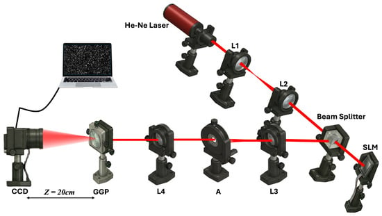
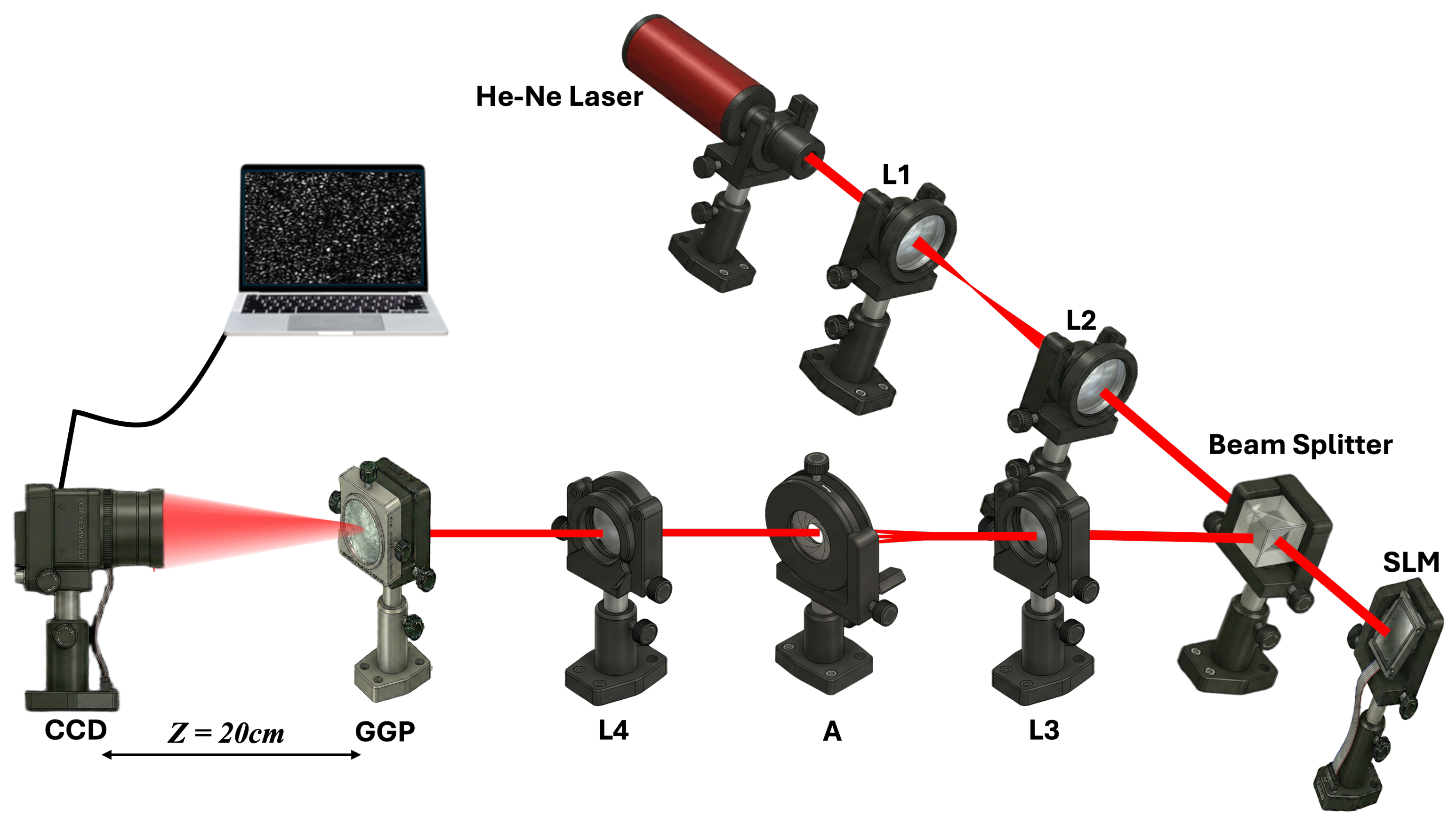
Figure 1 depicts the experimental setup in which linearly polarized light was produced using a 632.8 nm He-Ne laser source (5 mW, Thorlabs HRS015B). To expand the beam and ensure uniform illumination across the entire active area of the spatial light modulator (SLM) (Holoeye PLUTO 2.1, 1920 × 1080 pixels, 8 μm pixel pitch), a setup comprising two lenses, and , with focal lengths of 2.5 cm and 30 cm, respectively, was used. The expanded beam was then propagated through a cubic beam splitter and directed to SLM. Computer-generated holograms (CGHs) were loaded onto the SLM to modulate the phase of the incident wavefront, thus generating optical vortices with varying TC (ℓ = 0.0 to ℓ = 10.0 in continuous fractional increments of Δℓ) [51]. Mathematically, the field distribution of the FOV can be represented as the Fourier series of its integer vortex beams shown in Equation (1) [38]:
where denotes the field amplitude and is the fundamental Gaussian beam waist radius. The parameter m represents the TC of the fractional vortex beam, while ℓ indicates the integer vortex mode. The fractional TC is encoded by the weighting coefficient , which normalizes each associated integer mode [47].
Figure 1.
Schematic of the experimental optical setup for generating the fractional vortex beams and speckle patterns.
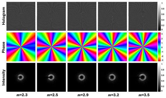
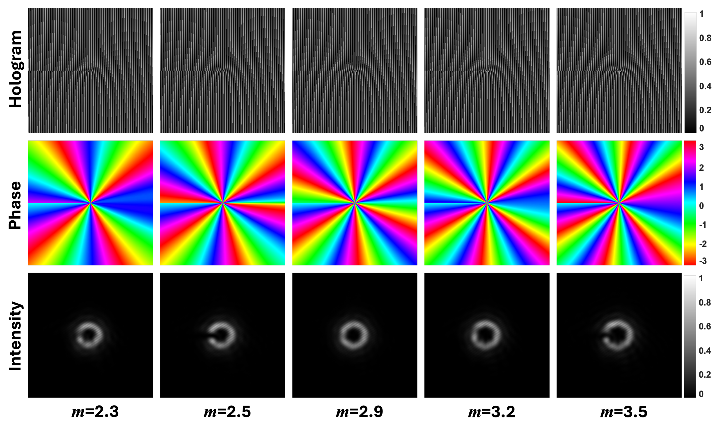
Upon reflection from the SLM, the phase-modulated beam carrying spatial mode passed back through the beam splitter, and we imaged the spatial modes using a 4f system (L3, L4; f = 30 cm) with an aperture filtering the first-order beam. Figure 2 illustrates some of the CGHs, along with the simulated resulting phase and the experimentally obtained intensity profiles of fractional spatial modes. The vortex beam then propagated towards a ground glass plate (GGP) (Thorlabs DG10-220, grit size 220) to generate speckle patterns. This scattered field caused by the GGP can be modeled as the 2D convolution of the incident input field and a random phase function introduced by the optical inhomogeneities of the GGP, denoted as )), which is expressed in Equation (2) [52]:
Figure 2.
Computer–generated holograms (top row) with their corresponding phase distributions (middle row) and resulting intensity profiles (bottom row) for various fractional topological charges.
These speckle patterns, captured using a charge-coupled device (CCD) camera (LT-LM11-M2420, resolution 2464 × 2056 pixels, pixel size 3.45 μm) with an exposure time of 10 ms and a gain of 1, were recorded as 8-bit grayscale intensity images for all values of m and serve as a dataset to detect fractional TC using the developed DL model.
3. Deep Learning Methodology
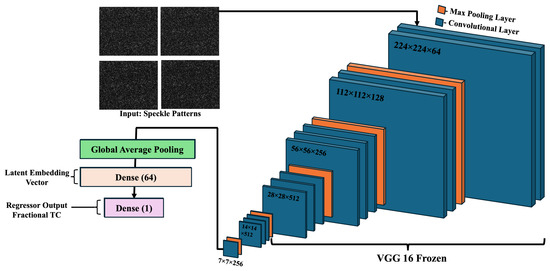
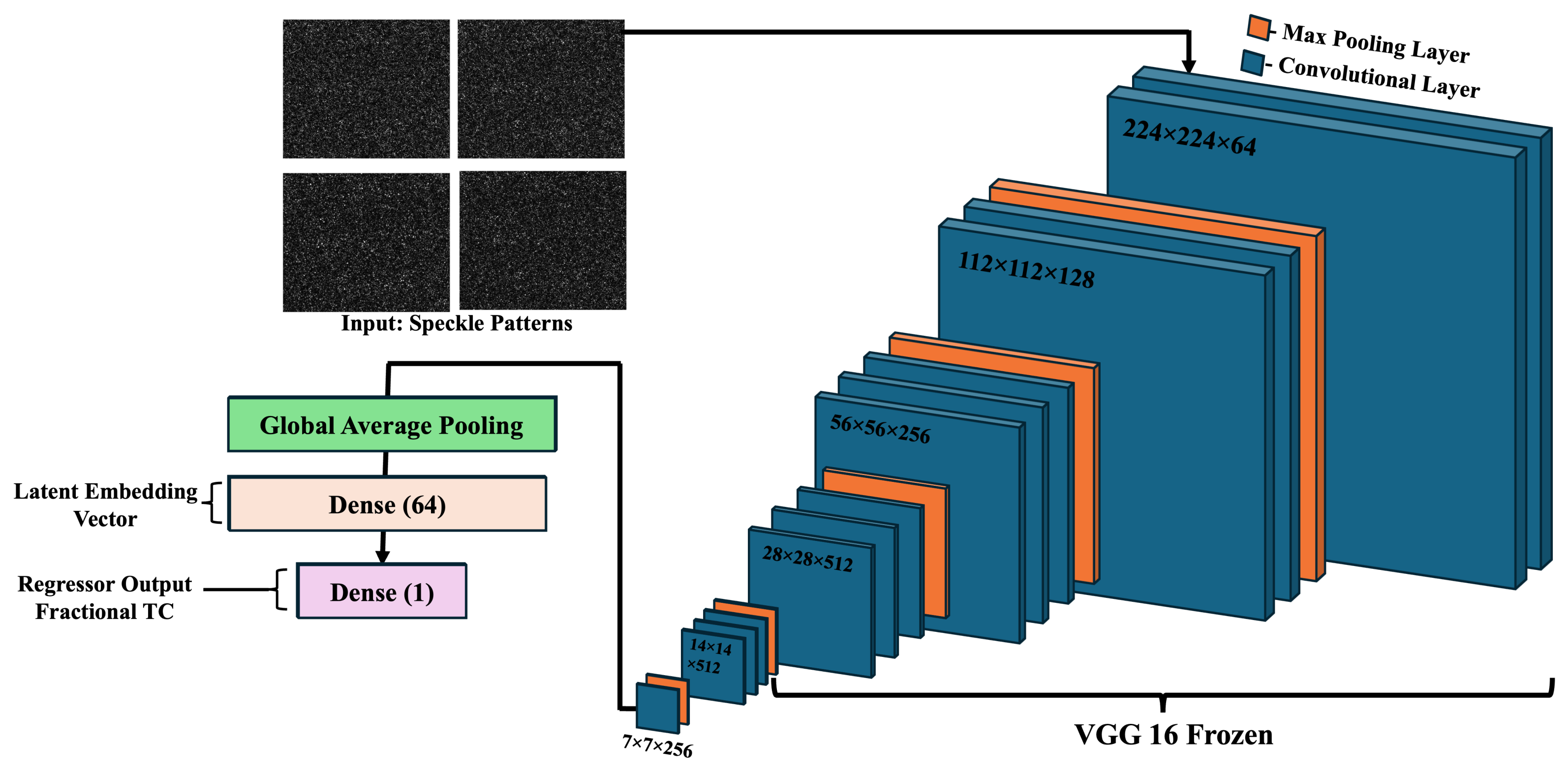
This section presents the complete DL framework, FT-VSRNet, which is used to detect the fractional TC ‘m’ from speckle patterns. Figure 3 shows the architecture of FT-VSRNet. This section further discusses the preparation of the fractional speckle dataset, the model architecture, the experimental design, and the evaluation metrics used to assess the model.
Figure 3.
Schematic of the FT-VSRNet architecture for detecting fractional TC from experimental speckle patterns.
3.1. Fractional Speckle Dataset
The experimental dataset used for FT-VSRNet comprises 9999 speckle images corresponding to 101 fractional topological charges (TCs), ranging from m = 0.0 to m = 10.0 with a fractional increment of (). For each fractional TC, 99 speckle images were generated by dividing an experimentally recorded 2464 × 2056 × 3 speckle image into 224 × 224 × 3 non-overlapping patches using an 11 × 9 spatial grid. The remaining 40 pixels along the vertical direction were excluded from the analysis. The speckle size is estimated from the width of the intensity autocorrelation, which varies with fractional TC and ranges from 70.56 μm (20.45 pixels) at to 23.58 μm (6.84 pixels) at . The spatial positions of patches were not provided to the FT-VSRNet, and only the intensity information within the patch was used as input to the proposed DL framework FT-VSRNet. All images were generated experimentally, with no simulated or synthetic speckle patterns, and no data augmentation was performed to ensure that spatial statistics were not altered. To ensure stability, the images were normalized by scaling the pixel values to [0, 1]. It should be noted that although the training, validation, and test patches are spatially non-overlapping, they were extracted from the same experimental image per fractional TC and were not fully independent acquisitions. Accordingly, this work demonstrates generalization across spatially separated speckle regions under the same experimental conditions, leaving acquisition-level generalization for future study.
3.2. FT-VSRNet Architecture
The network is primarily designed to map the spatial distribution of a speckle image to a continuous fractional TC (m). This network is basically a convolutional regression pipeline built in two functionally different stages: (1) a pretrained VGG-16 feature extraction backbone with selective fine-tuning and (2) a custom 4-layered regression head.
VGG-16 Backbone: The VGG-16 feature extraction backbone is a 16-layer architecture consisting of 5 sequential convolutional blocks, where each has a max pooling layer at the end for downsampling, followed by 3 fully connected layers [53]. The initialized weights are pretrained on the ImageNet Large-Scale Visual Recognition Challenge (1.2 million images, 1000 categories) [54]. In FT-VSRNet, the three original fully connected layers (FC-4096 × 2 and FC-1000) have been removed and replaced with a custom regression head. The rationale for choosing VGG-16 over what were then the most recent architectures is primarily based on 3 reasons. Firstly, it is a completely sequential block structure with no skip connections or attention mechanism, producing a spatially interpretable feature hierarchy. Second, its transfer learning effectiveness across image recognition, including texture-rich and low-contrast domains structurally similar to speckles, makes it a reliable backbone for fine-tuning. Lastly, the total parameter count (15.9 M) is large enough to represent the continuous morphological variation between classes representing fractional TC.
The VGG-16 backbone is subjected to selective fine-tuning where the first 15 layers (0–14), which are blocks 1 to 4, are frozen; the weights remain the same because they do not receive gradient updates during training. From layer 15, which is the starting point of block 5, it remains trainable. Such fine-tuning is performed to ensure that the early layers capture generic spatial-statistical features that transfer effectively to the speckle image, namely, structured interference patterns whose composition is encoded in their spatial-gradient statistics. However, the last layers are fine-tuned to remap onto the morphological features of fractional TC. The frozen backbone produces a 7 × 7 × 512 spatial feature map for each 224 × 224 × 3 input speckle image.
Custom Regression Head: The output of the VGG-16 backbone is followed by a 4-layer regression head that is used for fractional TC detection:
- 1.
- A 2D convolution operation is performed that involves the output of the VGG-16 backbone and 256 filters of kernel size 3 × 3 with a ReLU activation function, with the same padding to produce dimensions of 7 × 7 × 256. This layer is specifically used to capture the spatial co-localization of intensity gradients that encode the azimuthal symmetry breaking of the fractional TC and can be used for interpretability in future applications using XAI (Explainable AI) techniques. The output of this layer can be expressed aswhere ∗ denotes a 2D convolution operation, is a trainable weight filter, is a bias term and ReLU is a rectified linear unit activation function.
- 2.
- The refined spatial feature map is then passed through a global average pooling layer, which computes the spatial average of feature channels k, resulting in a feature vector v, which is a 256-dimensional vector. Here, can be expressed aswhere and are the spatial height and width of , which are 7 and 7 in this architecture, while i, j are indices for traversing the height and width of the feature map
- 3.
- To project the 256D vector into a 64D latent space, a dense layer with 64 neurons and ReLU activation is used. This embedding is used for PCA (Principal Component Analysis) visualization to check whether the latent space forms a smooth 1D manifold parameterized by ‘m’.
- 4.
- Finally, a single unit dense layer with linear activation is used to map the 64D space to a continuous scalar prediction ‘’.
3.3. Experimental Design
To verify and test whether the proposed model is learning the underlying phase transitions or merely memorizing patterns, the dataset was systematically used across 3 experimental design scenarios. The entire dataset consists of 101 distinct fractional TCs from to . Instead of varying the hyperparameters, our experimental design uses specific TCs for training and the rest for testing across various scenarios. Table 1, shown below, presents three scenarios that are evaluated to test the architecture and its interpolation capacity.
Table 1.
Experiment design and other parameters.
The choice of loss function in regression affects the model convergence, sensitivity to diverse TC values, and generalization behavior. As seen in Table 1, for experiment 1, where all 101 TCs are used to train and test and the errors are expected to be small, the absence of extrapolation makes mean square error (MSE) an optimal choice, as it penalizes the error quadratically. MSE loss is defined as
where is the predicted fractional TC, is the ground truth, and N is the number of samples in the batch. In experiments 2 and 3, the model must accurately interpolate the unseen TC in model testing; the use of MSE would generate quadratically growing gradients, which would destroy the manifold smoothness for interpolation. Huber loss, used here instead of MSE, resolves this by transitioning from a quadratic penalty (MSE) for small errors to a linear penalty (mean absolute error, or MAE) for large errors at threshold and is expressed as
where is the fractional TC predicted by the model, while is the true fractional TC.
To prevent overfitting and control convergence, an early stopping callback is implemented across all experiments, monitoring validation loss with a patience of 15 epochs and stopping training if no further improvement is observed within that window. A learning rate scheduler is integrated to manage convergence plateaus; specifically, the learning rate is halved (factor = 0.5) if the validation loss does not improve for four consecutive epochs, down to a minimum threshold of .
3.4. Evaluation Metrics
To test the predictive performance of FT-VSRNet, we evaluate the model using the following statistical metrics: MAE, MSE, root mean square error (RMSE), coefficient of determination (), and mean absolute percentage error (MAPE).
Let N denote the total number of speckle images in the test set, represent the true fractional TC of the speckle image and represent the fractional TC predicted by FT-VSRNet.
The characteristics of the metrics are as follows:
- 1.
- MAE provides an average absolute deviation between predicted and true TC. As it treats all errors equally, it is a reliable baseline for understanding a model’s average performance and is expressed in the same units as the target variable, i.e., TC. It is calculated using the following formula:
- 2.
- MSE provides a quadratic penalty for the prediction errors:
- 3.
- RMSE is directly derived from the square root of MSE:
- 4.
- The coefficient of determination (), used to evaluate the DL model’s predictive accuracy, measures the proportion of variance in m that is accounted for by the predictions of the model (). The coefficient is calculated as follows:where is the mean true TC in the test set.
- 5.
- Mean absolute percentage error (MAPE) calculates the average magnitude of the relative deviation between the predicted TC () and the ground-truth TC (m) expressed as a percentage, unlike MAE, which calculates the error in TC. MAPE is calculated as follows:
4. Results and Discussion
The objective of this study was to investigate whether the fractional TC can be inferred as a continuous physical parameter from speckle patterns, instead of being treated as a classification problem. All existing ML studies treat TC identification as a multi-class classification task. Although they have shown high accuracy for a predefined set of modes, they discretize TC, which is fundamentally continuous in nature. Treating TC detection as a classification problem, therefore, limits the ability of a system to resolve intermediate vortex states and restricts generalization to charges that were explicitly included in the training data. This limitation becomes significant in applications such as OAM multiplexing, where an accurate identification of vortex modes is required to demultiplex information channels. In such systems, fractional OAM states can serve either as intermediate symbols or as perturbations coming from propagation effects such as turbulence or scattering. A detection model capable of continuous TC estimation provides greater flexibility and robustness than classification methods. Here, we investigate whether the speckle pattern retains measurable statistical signatures of the vortex topology that can be used to directly regress the fractional TC.
The results presented in this section examine this capability in four stages. We first present a fully supervised fractional TC regression model, which is trained on the complete charge continuum and predicts TC as a continuous scalar. We then explore and represent a more challenging scenario in which the network is trained on sparsely sampled vortex orders and is required to infer intermediate fractional charges that were never observed during training. This setting effectively evaluates the model’s ability and capacity to perform interpolation across the vortex charge manifold, enabling prediction of previously unseen fractional TC between sparsely sampled training data. Next, we present a comparative study with alternate regression models. Finally, we present the physical basis for continuous TC regression through interpolable speckle statistics.
4.1. Fully Supervised Fractional TC Regression
Here, FT-VSRNet is trained on the complete fractional TC space. The experimental dataset consists of speckle patterns corresponding to 101 vortex states spanning to with increments of (). Data were divided using a stratified 80/10/10 split for training, validation, and testing, respectively, to preserve the distribution of TC values across the splits. FT-VSRNet minimizes the error to achieve a precise prediction of the fractional topological charge. This sets the model’s intrinsic performance ceiling when the entire range of fractional TCs is used for training.
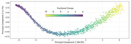
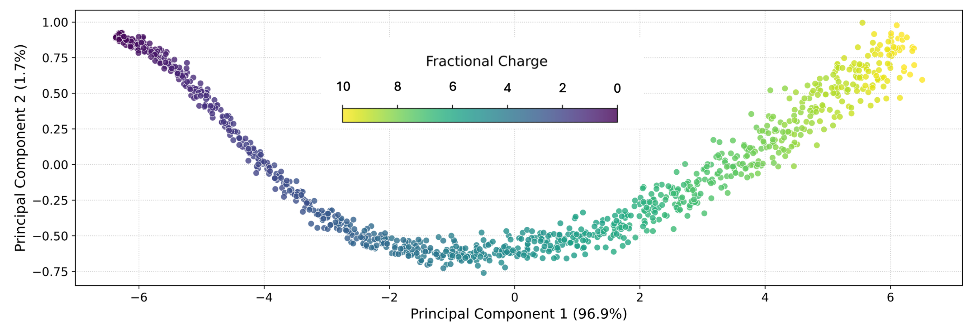
Before analyzing evaluation metrics, it is useful to examine how the model internally represents speckle patterns. FT-VSRNet transforms each speckle image into a 64-dimensional latent feature vector, a compressed representation of the spatial interference statistics in the speckle pattern. To visualize the latent features extracted from multiple speckle patterns, they were projected onto a two-dimensional space using PCA; the latent feature space is shown in Figure 4, where each point corresponds to a captured speckle pattern and the color scale represents the associated fractional TC.
Figure 4.
PCA visualization of the 64-dimensional latent space.
It is evident from this PCA visualization that feature representations form a smooth and continuous trajectory, with the ordering of points closely following the magnitude of fractional TC. Instead of forming isolated clusters corresponding to discrete TC values, they show a gradual progression as TC increases. This observation is consistent with the continuous regression formulation. However, PCA alone cannot establish the physical origin of the learned features or exclude acquisition specific characteristics. Thus, the latent space is interpreted as supporting evidence of a continuous TC-dependent representation, whose physical basis is discussed in Section 4.4.
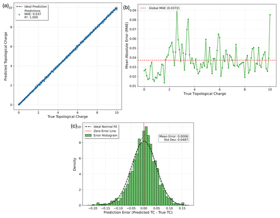
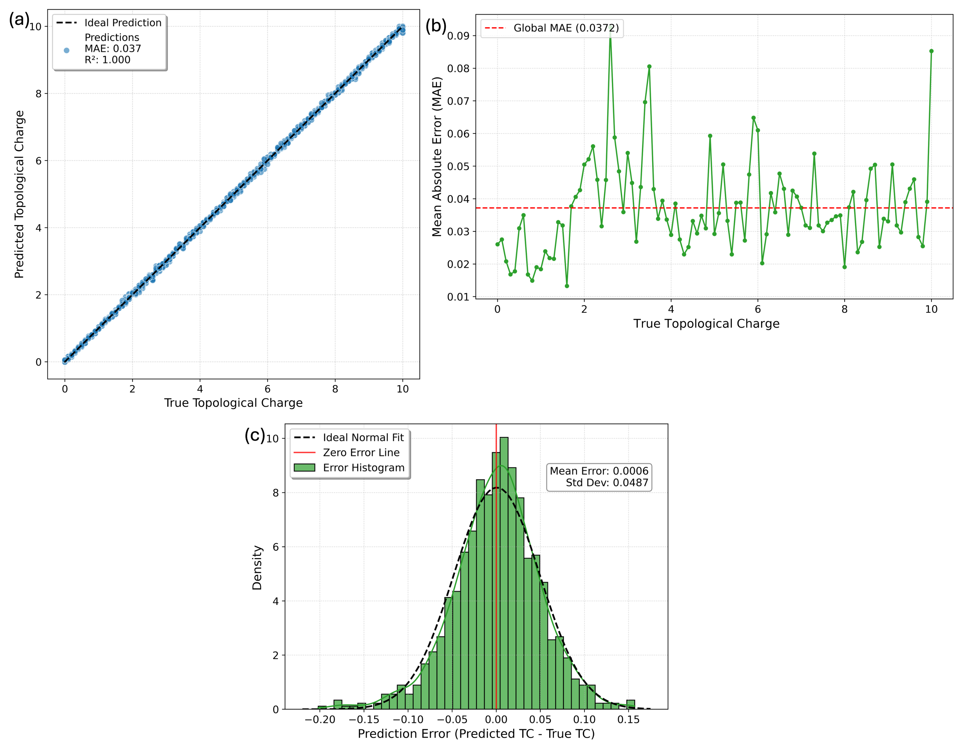
The performance of the model was evaluated by comparing the predicted TC () with the actual TC (m), as shown in Figure 5a. The dashed line represents the ideal prediction (); here, the predicted values closely follow the ideal linear relation, and the extremely small deviation from the ideal prediction is reflected in the regression metrics. Across three independent training runs with different random seeds, the fully supervised model achieved an MAE of , an RMSE of , and an of , as summarized in Table 2. The small standard deviations indicate that the regression performance is stable with respect to stochastic variations in model initialization and training. Figure 5b analyzes the robustness of the model in various orders by plotting the MAE against the true TC, where the dashed horizontal line denotes the global MAE; the error values fluctuate slightly around this global average but remain relatively uniform. Specifically, no systematic increase in prediction error is observed in higher vortex orders. The distribution of prediction residuals () is shown in Figure 5c, where the histogram is an approximately Gaussian distribution; this symmetric distribution around 0 indicates that the model does not show a systematic tendency to overestimate or underestimate the TC.
Figure 5.
Statistical evaluation of fractional TC prediction for a representative training run. (a) Correlation between true and predicted TC; (b) MAE plotted against TC (m); (c) histogram of prediction residuals or error ().
Table 2.
Performance metrics for the fully supervised fractional TC regression across three independent runs.
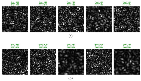
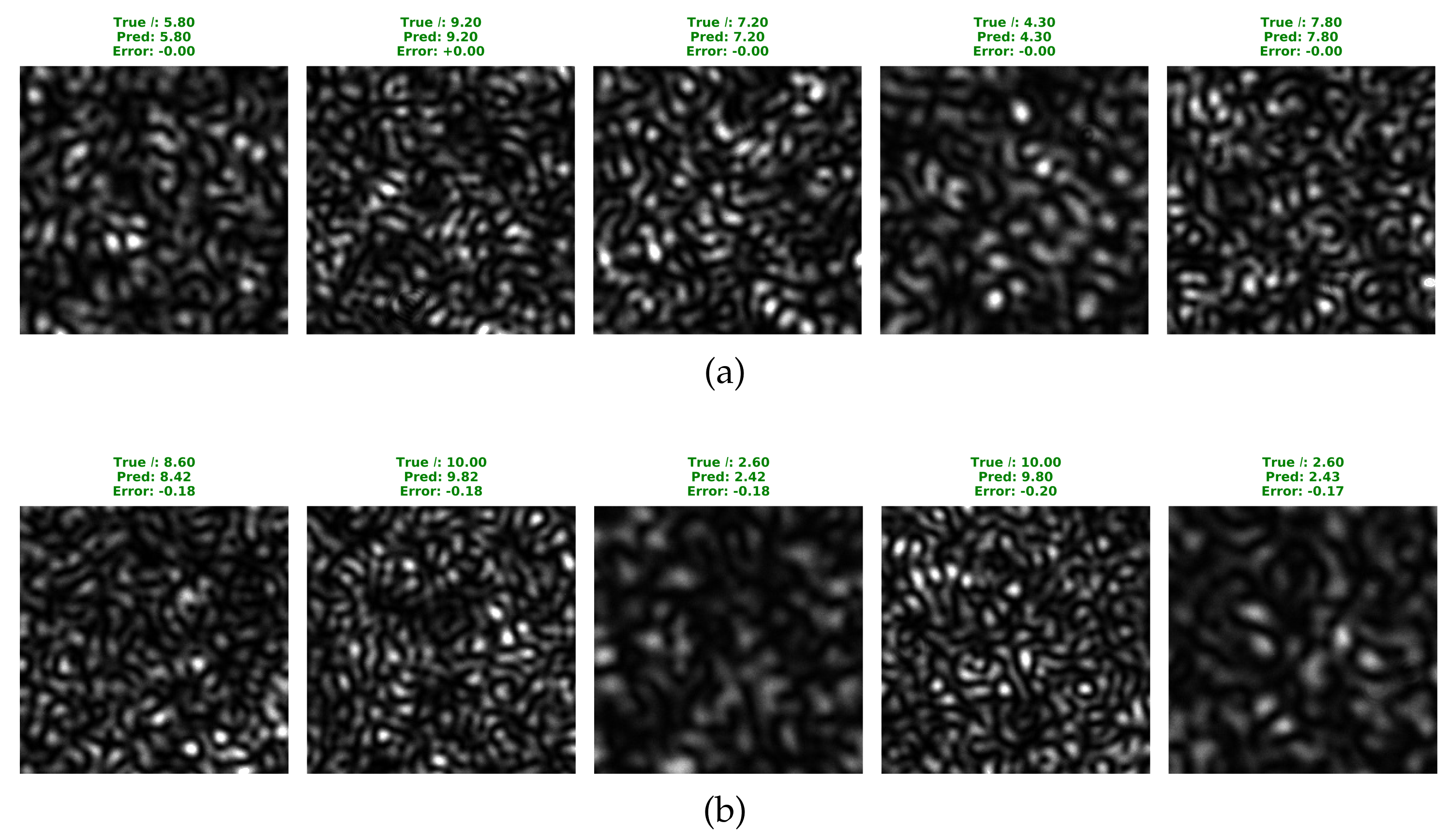
Beyond the metrics presented in Table 2, which provide an overall measure of the performance of the model, Figure 6a,b show the model performance through five best and five worst predictions. The absolute error for the best cases is ≈0, showing that the prediction is extremely precise and nearly perfect; even in the worst case, the absolute error is 0.2, where the true order was 10.
Figure 6.
Representative speckles from the fully supervised regression test set showing the predictive performance of FT−VSRNet. (a) Top 5 best predictions, showing excellent agreement between predicted () and true (m) fractional TC. (b) Top 5 worst predictions (maximum absolute error = 0.2018).
4.2. Interpolation of Unseen Fractional Topological Charges
Experimentally capturing speckle patterns for every fractional TC (e.g., ) across a wide range is often resource intensive and impractical, requiring precise SLM control, repeated alignment, and considerable acquisition time, with added difficulty in turbulent environments. Training on every possible fractional charge is, therefore, neither scalable nor realistic for implementation (deployment realistic). Instead, we opt for the more realistic and robust approach of training on a sparse set of anchor points and leveraging the model’s ability to interpolate the unseen intermediate fractional TC.
For evaluation, Experimental Scenarios 2 and 3 were conducted, in which FT-VSRNet was trained on sparse TC charges and tested on completely unseen intermediate fractional TCs within . Performance metrics for Experiments 2 and 3 are summarized in Table 3 across three independent training runs.
Table 3.
Overall performance metrics for Experiments 2 and 3 across three independent training runs.
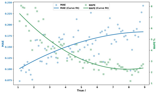
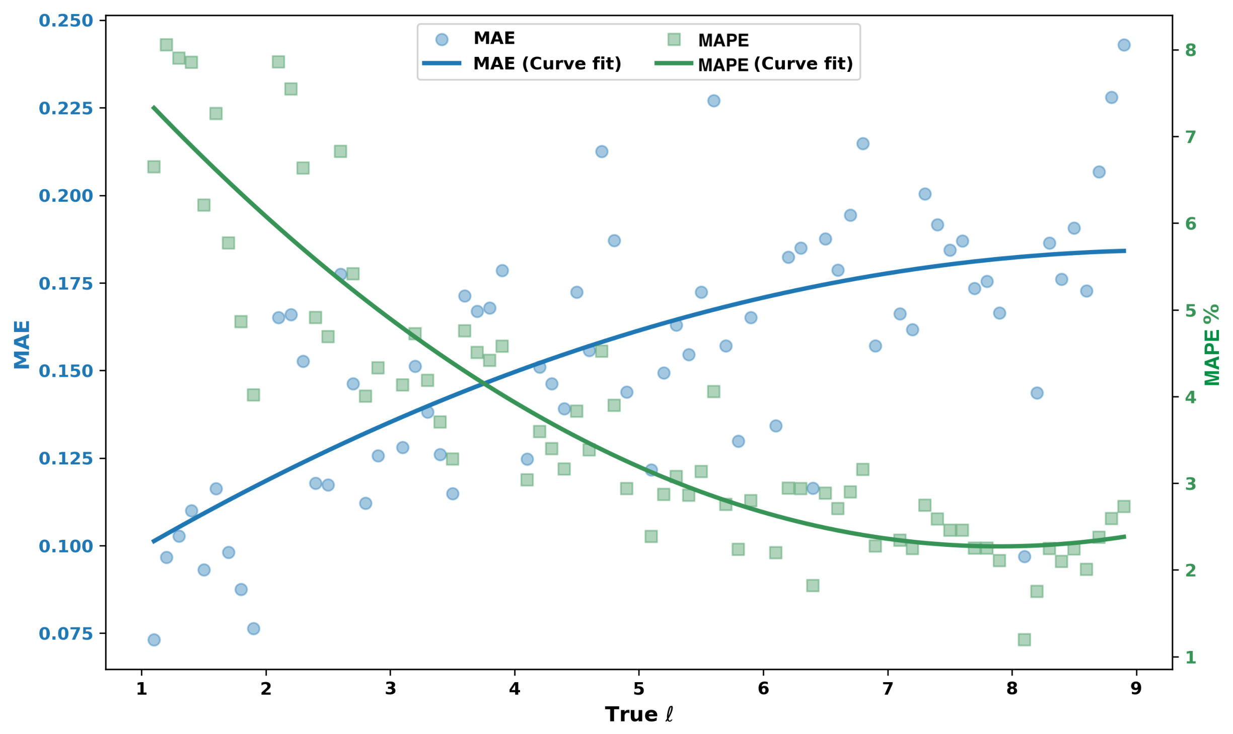
When trained only on 11 integer charges (Experimental Scenario 2), the model achieves an MAE of , an RMSE of , and an of across three independent runs. The small standard deviations indicate that the interpolation performance is stable with respect to stochastic variations in model initialization and training. This strong generalization is because the speckle patterns corresponding to neighboring fractional charges have highly correlated spatial statistics. Despite being trained only on integer TCs, it captures the phase-induced azimuthal symmetry breaking that governs the continuous transition between integer and fractional vortices, allowing it to interpolate the unseen intermediate fractional TC with ≈0.15 MAE. The TC-dependent error plot is shown in Figure 7, where the MAE shows a gradual increase as the TC increases, and the curve fit shows that the predictive error remains relatively small at lower TC but grows slightly at higher TC. This behavior can be interpreted as follows: as the TC increases, the number of azimuthal phase windings increases, and the scattered field develops an increasingly complex interference field. However, MAPE decreases with increasing TC, indicating that the relative error decreases with TC because the absolute deviation in predicted TC becomes proportionally less significant. Overall, the evaluation metrics, along with the smooth curve, indicate that the model can interpolate intermediate fractional TCs, even when trained solely on integer TCs.
Figure 7.
Charge-resolved MAE and MAPE for Experiment 2 (training on integer charges only).
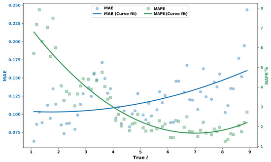
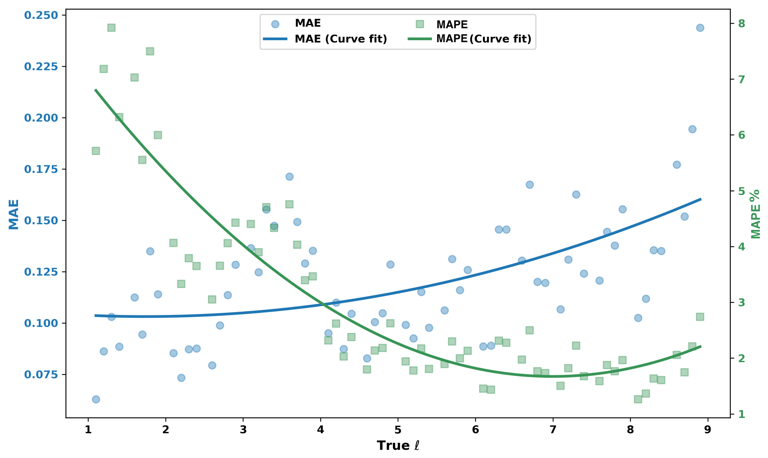
When the training set is further enriched by including half-integer TCs (x.5) (Experimental Scenario 3) it reduces the MAE to 0.120, improving performance; the error against the TC plot is shown in Figure 8, where the MAE curve becomes noticeably flatter and decreases compared to Experimental Scenario 2 (Figure 7), implying that the prediction remains more consistent across the TC range. The MAPE decreases similarly with increasing charge but exhibits smaller fluctuations than in Experimental Scenario 2 (Figure 7). This reduction shows that additional training data enable the model to better capture the evolution of speckle morphology with respect to the fractional TC.
Figure 8.
Charge-resolved MAE and MAPE for Experiment 3 (training on integer and half-integer charges).
When the training set was further enriched by including half-integer TCs (x.5) (Experimental Scenario 3), the MAE decreased to , with an RMSE of and across three independent runs, reflecting improved performance; the error against the TC plot is shown in Figure 8, where the MAE curve becomes noticeably flatter and decreases compared to Experimental Scenario 2 (Figure 7), implying that the prediction remains more consistent across the TC range. The MAPE decreases similarly with increasing charge but exhibits smaller fluctuations than in Experimental Scenario 2 (Figure 7). This reduction shows that additional training data enable the model to better capture the evolution of speckle morphology with respect to the fractional TC.
4.3. Comparative Study with Alternative Regression Architectures
To further evaluate the performance of the proposed model FT-VSRNet and to determine whether its regression capability is primarily associated with the use of a pretrained convolutional backbone or with the specific architectural design, a comparative study was performed using two widely used CNN architectures, ResNet50 and EfficientNet-B0 [55,56]. Both models were initialized with ImageNet-pretrained weights and were adapted for continuous fractional TC regression. To maintain a controlled comparison, the input speckle images, experimental training scenarios, evaluation metrics, and other parameters were kept same as those used for FT-VSRNet.
- For the ResNet50-based regression model, the ImageNet-pretrained ResNet50 backbone was used as a feature extractor. The earlier convolutional stages were frozen, while the final residual stage (layer 4) was fine-tuned together with the custom regression head. This selective fine-tuning allows the pretrained low-level spatial features to be preserved while adapting the high-level representation to the speckle statistics related to fractional TC.
- For the EfficientNet-B0-based regression model, ImageNet-pretrained weights were used similarly for initialization. The earlier feature extraction blocks were frozen, while the final three MBConv feature blocks were fine-tuned together with the custom regression head. EfficientNet-B0 is known for providing a computationally efficient convolutional feature representation through its compound scaled architecture and mobile inverted convolution (MBConv)-based feature extraction.
For both alternative architectures, the final classification layers of the pretrained models were replaced with the same custom regression head used for the comparison. Thus, the primary difference between the comparison models and FT-VSRNet is the backbone and its corresponding fine-tuning strategy, while the custom regression head remains the same. The three models were evaluated under the same three experimental scenarios described earlier in Section 3.3.
The comparative results shown in Table 4 show that FT-VSRNet consistently provides the strongest regression performance in all three experiments. In the fully supervised scenario of Experiment 1, FT-VSRNet achieves an MAE of , compared to for ResNet50 and for EfficientNet-B0. It also has the lowest RMSE and the highest , showing that the advantage is not limited to a single evaluation metric. A similar trend can be observed when the models are used to interpolate unseen fractional TCs. In Experiment 2, FT-VSRNet achieves an MAE of , while EfficientNet-B0 and ResNet50 have MAEs of and , respectively. The corresponding MAPE values further show the lower relative prediction error of FT-VSRNet. In Experiment 3, the performance of all three models improves; however, FT-VSRNet continues to provide the lowest MAE, MSE, RMSE, and MAPE and the highest . The consistent order of performance, FT-VSRNet > EfficientNet-B0 > ResNet50, across the three experiments indicates that the observed performance of FT-VSRNet is not merely a consequence of using an ImageNet-pretrained convolutional backbone. Instead, the results support the effectiveness of the specific VGG-16-based feature extraction and custom regression head with selective fine-tuning used in FT-VSRNet. The larger performance gap observed in interpolation experiments is especially significant, as it shows that the architectural design is effective not only when all fractional TC samples are available during training but also when the model must infer intermediate charges from sparse data. Although this comparative analysis evaluates alternative backbones under controlled fine-tuning conditions, a dedicated ablation isolating the individual contributions of the custom regression head and selective fine-tuning remains for future work.
Table 4.
Comparative performance of FT-VSRNet, ResNet50, and EfficientNet-B0 for fractional TC regression.
4.4. Physical Basis for Continuous TC Regression via Interpolable Speckle Statistics
The results of Experiments 2 and 3 show that even when trained on sparsely sampled TCs, the model has the capacity to interpolate intermediate fractional charges by leveraging the continuity of speckle statistics related to the evolving phase structure of the incident beam. This gradual reduction in error as the anchor density (size of the training set) increases confirms that FT-VSRNet captures the continuous nature of fractional TC. Although a speckle pattern has random intensity distribution, FT-VSRNet performs successfully as a continuous regressor due to the underlying structure of the fractional vortex field, allowing the pattern to encode a smoothly interpolable signature of m. According to Berry’s theory of fractional optical vortices, a beam carrying fractional TC m is not an independent spatial mode but a coherent superposition of neighboring integer OAM modes ℓ, weighted by the coefficient (Equation (1)) [38]. For fixed integer mode ℓ, the coefficient varies smoothly with m, with no abrupt discontinuity in the field as m sweeps through non-integer values, only a continuous redistribution of optical power among neighboring integer modes.
Consequently, increasing the charge does not generate an entirely new optical mode; instead, it produces a gradual evolution of the phase singularity, the radial phase discontinuity, and the overall complex wavefront. Furthermore, Leach et al. experimentally showed that a fractional vortex beam resolves into a finite chain of unit-strength vortex lines whose number and angular position evolve continuously with m, manifested as a radial dark notch that breaks the annular intensity rings [39]. When such a field is scattered through the GGP, the resulting random speckle patterns carry this continuous evolution through the scattering process, and the higher-order spatial correlation within the speckles evolves continuously because it remains governed by the continuously varying modal coefficients . This behavior is consistent with the observations of Ansari et al. [47], who showed that the autocorrelation of speckle patterns exhibits asymmetric ring profiles for fractional TCs and symmetric profiles for integer TCs, with the asymmetry continuously approaching symmetry as fractional TCs approach the next integer. Their results demonstrate that the statistical structure of the speckles evolves smoothly with the fractional TC despite the presence of scattering. Consequently, neighboring fractional charges produce highly correlated speckle patterns, whereas larger charge differences lead to progressively greater statistical variation. This physical continuity is reflected in the smooth trajectory observed in the latent feature space (Figure 4), where features of speckle patterns corresponding to neighboring fractional TCs are mapped nearby. The learned representation primarily reflects the fractional-TC-dependent statistical structure of the speckles rather than a certain position of the GGP, since the model is trained using the spatial intensity statistics of the scattered field and is not directly provided with information about the scattering geometry or GGP position. However, changes in diffuser position, orientation, scattering strength, or propagation geometry can modify the speckle statistics. The present study does not experimentally quantify this invariance; therefore, validation across independently varied scattering configurations is left for future study.
Instead of treating each TC as a separate class, FT-VSRNet learns the continuous relationship between speckle patterns and fractional TC. Since this relationship changes smoothly over the entire TC range, the model can accurately interpolate between sparsely sampled training points. As a result, when trained only on integer or integer-plus-half-integer TCs (Experimental Scenarios 2 and 3), FT-VSRNet successfully predicts unseen intermediate fractional TCs, demonstrating accurate interpolation between sparsely sampled training data. These results are consistent with the model exploiting the continuous evolution of speckle statistics with fractional TCs, rather than simply memorizing the statistical patterns found in training data and treating each training TC as a separate class. The ability to estimate intermediate fractional TCs that are not present in the training data provides evidence that the learned representation captures a TC-dependent relationship that extends between the discrete training TC values. These results show the potential relevance of continuous fractional TC estimation to applications such as OAM-based optical communication, optical manipulation, and high-dimensional quantum information processing, where accurate detection of the optical mode is important. However, the present study does not evaluate application-specific performance metrics, and further validation under realistic conditions is necessary.
5. Conclusions
The FT-VSRNet model learns the relationship between speckle statistics and phase, allowing the estimation of TC as a continuous parameter rather than a discrete class. FT-VSRNet achieves high predictive accuracy when trained on the entire TC range (MAE , ) and demonstrates strong interpolation capabilities (MAE , ) even when trained only on sparse TC values. The smooth latent space and a gradual reduction in error with an increase in training TC data support the ideas that speckle patterns retain information about vortex topology and that the model can be leveraged for reliable TC estimation. This passive, non-interferometric approach bypasses the limitations of traditional interferometric and diffractive techniques and addresses the practical difficulty of exhaustive fractional TC calibration. The demonstrated continuous estimation of fractional TC may have potential relevance to applications involving fractional-OAM multiplexing in optical communication, precision optical manipulation, and high-dimensional quantum information processing. However, application-specific validation under realistic conditions remains necessary to confirm the suitability of the achieved TC estimation accuracy.
Author Contributions
Conceptualization, S.S.M. and S.G.R.; methodology, S.S.M.; software, S.S.M. and S.A.; validation, S.S.M. and M.H.A.; formal analysis, S.S.M., G.M.B. and R.K.; investigation, S.S.M., M.H.A. and S.G.R.; resources, S.A. and S.G.R.; data curation, M.H.A. and G.V.; writing—original draft preparation, S.S.M. and M.H.A.; writing—review and editing, S.A., G.M.B., R.K. and S.G.R.; visualization, S.S.M., M.H.A., G.V. and G.M.B.; supervision, S.A., R.K. and S.G.R.; project administration, S.G.R.; funding acquisition, S.G.R. All authors have read and agreed to the published version of the manuscript.
Funding
S.G.R. acknowledges the financial support from ISRO under the RESPOND Basket with sanction order ISRO/RES/3/958/24-25.
Data Availability Statement
The dataset is available on request from the authors.
Conflicts of Interest
The authors declare no conflicts of interest.
Abbreviations
The following abbreviations are used in this manuscript:
| ANN | Artificial Neural Network |
| CNN | Convolutional Neural Network |
| DNN | Deep Neural Network |
| DL | Deep Learning |
| LG | Laguerre–Gaussian |
| ML | Machine Learning |
| MSE | Mean Squared Error |
| OAM | Orbital Angular Momentum |
| OV | Optical Vortex |
| RMSE | Root Mean Square Error |
| SLM | Spatial Light Modulator |
| TC | Topological Charge |
References
- Allen, L.; Beijersbergen, M.W.; Spreeuw, R.; Woerdman, J. Orbital angular momentum of light and the transformation of Laguerre-Gaussian laser modes. Phys. Rev. A 1992, 45, 8185. [Google Scholar] [CrossRef] [Scilit] [PubMed]
- Yu, S. Potentials and challenges of using orbital angular momentum communications in optical interconnects. Opt. Express 2015, 23, 3075–3087. [Google Scholar] [CrossRef] [Scilit] [PubMed]
- Wang, J.; Yang, J.Y.; Fazal, I.M.; Ahmed, N.; Yan, Y.; Huang, H.; Ren, Y.; Yue, Y.; Dolinar, S.; Tur, M.; et al. Terabit free-space data transmission employing orbital angular momentum multiplexing. Nat. Photonics 2012, 6, 488–496. [Google Scholar] [CrossRef] [Scilit]
- Fu, S.; Zhai, Y.; Zhou, H.; Zhang, J.; Yin, C.; Gao, C. Demonstration of high-dimensional free-space data coding/decoding through multi-ring optical vortices. Chin. Opt. Lett. 2019, 17, 080602. [Google Scholar] [CrossRef] [Scilit]
- Fürhapter, S.; Jesacher, A.; Bernet, S.; Ritsch-Marte, M. Spiral phase contrast imaging in microscopy. Opt. Express 2005, 13, 689–694. [Google Scholar] [CrossRef] [Scilit] [PubMed]
- Balasubramaniam, G.M.; Allam, S.R.; Anand, V.; Ansari, M.H.; Arockiaraj, F.G.; Arnon, S.; Badavath, P.S.; Baliyan, M.; Bouchal, P.; Bouchal, Z.; et al. Roadmap on Singular Optics and Its Applications. Appl. Phys. B 2026, 132, 58. [Google Scholar] [CrossRef] [Scilit] [PubMed]
- Mair, A.; Vaziri, A.; Weihs, G.; Zeilinger, A. Entanglement of the orbital angular momentum states of photons. Nature 2001, 412, 313–316. [Google Scholar] [CrossRef] [Scilit] [PubMed]
- Fickler, R.; Campbell, G.; Buchler, B.; Lam, P.K.; Zeilinger, A. Quantum entanglement of angular momentum states with quantum numbers up to 10,010. Proc. Natl. Acad. Sci. USA 2016, 113, 13642–13647. [Google Scholar] [CrossRef] [Scilit] [PubMed]
- Balasubramaniam, G.M.; Kumar, R.; Arnon, S. Vortex Beams and Deep Learning for Optical Wireless Communication Through Turbulent and Diffuse Media. J. Light. Technol. 2024, 42, 3631–3641. [Google Scholar] [CrossRef] [Scilit]
- Dholakia, K.; Macdonald, M.; Spalding, G. Optical tweezers: The next generation. Phys. World 2002, 15, 31. [Google Scholar] [CrossRef] [Scilit]
- Grier, D.G. A revolution in optical manipulation. Nature 2003, 424, 810–816. [Google Scholar] [CrossRef] [Scilit] [PubMed]
- Gao, B.; Wen, J.; Zhu, G.; Ye, L.; Wang, L.G. Precise measurement of trapping and manipulation properties of focused fractional vortex beams. Nanoscale 2022, 14, 3123–3130. [Google Scholar] [CrossRef] [Scilit] [PubMed]
- Tao, S.; Yuan, X.; Lin, J.; Peng, X.; Niu, H. Fractional optical vortex beam induced rotation of particles. Opt. Express 2005, 13, 7726–7731. [Google Scholar] [CrossRef] [Scilit] [PubMed]
- Zhen, W.; Wang, X.L.; Ding, J.; Wang, H.T. Controlling the symmetry of the photonic spin Hall effect by an optical vortex pair. Phys. Rev. A 2023, 108, 023514. [Google Scholar] [CrossRef] [Scilit]
- Ul Haq, Z.; Ahmad, I.; Bacha, B.A.; Akgül, A.; Hassani, M.K. Coherent manipulation of Goos–Hänchen shifts by forward and backward currents of complex conductivity in chiral medium. Sci. Rep. 2025, 15, 13348. [Google Scholar] [CrossRef] [Scilit] [PubMed]
- Zhen, W.; Ren, Z.C.; Wang, X.L.; Ding, J.; Wang, H.T. Polarization structure transition of C-point singularities upon reflection. Sci. China Phys. Mech. Astron. 2025, 68, 244211. [Google Scholar] [CrossRef] [Scilit]
- Zhao, Q.; Dong, M.; Bai, Y.; Yang, Y. Measuring high orbital angular momentum of vortex beams with an improved multipoint interferometer. Photonics Res. 2020, 8, 745–749. [Google Scholar] [CrossRef] [Scilit]
- Deng, D.; Lin, M.; Li, Y.; Zhao, H. Precision measurement of fractional orbital angular momentum. Phys. Rev. Appl. 2019, 12, 014048. [Google Scholar] [CrossRef] [Scilit]
- Qi, S.; Liu, S.; Han, L.; Wei, B.; Li, P.; Zhong, J.; Guo, X.; Zhao, J. Dynamically measuring the holo-information of light fields in three-dimensional space using a periodic polarization-structured light. Sci. China Phys. Mech. Astron. 2021, 64, 264211. [Google Scholar] [CrossRef] [Scilit]
- Zhou, G.; Wang, X.; Dai, C.; Chu, X. Angular momentum density of a Gaussian vortex beam. Sci. China Phys. Mech. Astron. 2014, 57, 619–627. [Google Scholar] [CrossRef] [Scilit]
- Shen, D.; Zhao, D. Measuring the topological charge of optical vortices with a twisting phase. Opt. Lett. 2019, 44, 2334–2337. [Google Scholar] [CrossRef] [Scilit] [PubMed]
- Leach, J.; Padgett, M.J.; Barnett, S.M.; Franke-Arnold, S.; Courtial, J. Measuring the orbital angular momentum of a single photon. Phys. Rev. Lett. 2002, 88, 257901. [Google Scholar] [CrossRef] [Scilit] [PubMed]
- Chen, L.; Singh, R.K.; Dogariu, A.; Chen, Z.; Pu, J. Estimating topological charge of propagating vortex from single-shot non-imaged speckle. Chin. Opt. Lett. 2021, 19, 022603. [Google Scholar] [CrossRef] [Scilit]
- Avramov-Zamurovic, S.; Esposito, J.M.; Nelson, C. Classifying beams carrying orbital angular momentum with machine learning: Tutorial. J. Opt. Soc. Am. A 2022, 40, 64–77. [Google Scholar] [CrossRef] [Scilit] [PubMed]
- Zhang, L.F.; Lin, Y.Y.; She, Z.Y.; Huang, Z.H.; Li, J.Z.; Luo, X.; Yan, H.; Huang, W.; Zhang, D.W.; Zhu, S.L. Recognition of orbital-angular-momentum modes with different topological charges and their unknown superpositions via machine learning. Phys. Rev. A 2021, 104, 053525. [Google Scholar] [CrossRef] [Scilit]
- Sun, R.; Guo, L.; Cheng, M.; Li, J.; Yan, X. Identifying orbital angular momentum modes in turbulence with high accuracy via machine learning. J. Opt. 2019, 21, 075703. [Google Scholar] [CrossRef] [Scilit]
- Wang, J.; Wang, C.; Tan, Z.; Wang, X.; Lei, S.; Wu, P.; Yang, C. Detection of orbital angular momentum carried high-order radial vortex beams using CNN-OAM mode classifier. Opt. Laser Technol. 2024, 169, 110027. [Google Scholar] [CrossRef] [Scilit]
- Zhao, Q.; Hao, S.; Wang, Y.; Wang, L.; Xu, C. Orbital angular momentum detection based on diffractive deep neural network. Opt. Commun. 2019, 443, 245–249. [Google Scholar] [CrossRef] [Scilit]
- Li, X.; Sun, L.; Huang, J.; Zeng, F. Research on orbital angular momentum recognition technology based on a convolutional neural network. Sensors 2023, 23, 971. [Google Scholar] [CrossRef] [Scilit] [PubMed]
- Zhou, J.; Yin, Y.; Tang, J.; Ling, C.; Cao, M.; Cao, L.; Liu, G.; Yin, J.; Xia, Y. Recognition of high-resolution optical vortex modes with deep residual learning. Phys. Rev. A 2022, 106, 013519. [Google Scholar] [CrossRef] [Scilit]
- Neary, P.L.; Watnik, A.T.; Judd, K.P.; Lindle, J.R.; Flann, N.S. CNN classification architecture study for turbulent free-space and attenuated underwater optical OAM communications. Appl. Sci. 2020, 10, 8782. [Google Scholar] [CrossRef] [Scilit]
- Raskatla, V.; Kumar, V. Deep learning assisted OAM modes demultiplexing. In Proceedings of the Fifteenth International Conference on Correlation Optics; SPIE: Bellingham, WA, USA, 2021; Volume 12126, pp. 73–78. [Google Scholar]
- Merabet, B.; Liu, B.; Li, Z.; Tian, J.; Guo, K.; Shah, S.A.A.; Guo, Z. Vision transformers motivating superior OAM mode recognition in optical communications. Opt. Express 2023, 31, 38958–38969. [Google Scholar] [CrossRef] [Scilit] [PubMed]
- Merabet, B.; Li, L.; Shah, S.A.A.; Guo, Z. Quantum Neural Network Boosting Identifying Orbital Angular Momentum Modes. Adv. Quantum Technol. 2025, 8, 2400680. [Google Scholar] [CrossRef] [Scilit]
- Raskatla, V.; Singh, B.P.; Patil, S.; Kumar, V.; Singh, R. Speckle-based deep learning approach for classification of orbital angular momentum modes. J. Opt. Soc. Am. A 2022, 39, 759–765. [Google Scholar] [CrossRef] [Scilit] [PubMed]
- Raskatla, V.; Badavath, P.S.; Kumar, V. Convolutional networks for speckle-based orbital angular momentum modes classification. Opt. Eng. 2022, 61, 036114. [Google Scholar] [CrossRef] [Scilit]
- Du, H.b.; Chen, J.; Li, Y.s.; Fu, G.k.; Wang, H.l.; Shi, Y.; Zhao, C.l.; Jin, S.z. Recognition of orbital angular momentum modes based on deep learning and multiaperture speckle. Optik 2023, 285, 170953. [Google Scholar] [CrossRef] [Scilit]
- Berry, M. Optical vortices evolving from helicoidal integer and fractional phase steps. J. Opt. A Pure Appl. Opt. 2004, 6, 259–268. [Google Scholar] [CrossRef] [Scilit]
- Leach, J.; Yao, E.; Padgett, M.J. Observation of the vortex structure of a non-integer vortex beam. New J. Phys. 2004, 6, 71. [Google Scholar] [CrossRef] [Scilit]
- Zhang, H.; Zeng, J.; Lu, X.; Wang, Z.; Zhao, C.; Cai, Y. Review on fractional vortex beam. Nanophotonics 2022, 11, 241–273. [Google Scholar] [CrossRef] [Scilit] [PubMed]
- Wang, J.; Zhang, W.; Qi, Q.; Zheng, S.; Chen, L. Gradual edge enhancement in spiral phase contrast imaging with fractional vortex filters. Sci. Rep. 2015, 5, 15826. [Google Scholar] [CrossRef] [Scilit] [PubMed]
- Situ, G.; Warber, M.; Pedrini, G.; Osten, W. Phase contrast enhancement in microscopy using spiral phase filtering. Opt. Commun. 2010, 283, 1273–1277. [Google Scholar] [CrossRef] [Scilit]
- Fan, W.; Chen, T.; Tang, X.; Xu, X.; Yuan, L.; Yakovlev, V.V.; Zhu, S.Y.; Wang, D.W.; Zhang, D. Spatial multiplexing for robust optical vortex transmission with optical nonlinearity. Opt. Express 2023, 31, 31610–31621. [Google Scholar] [CrossRef] [Scilit] [PubMed]
- Krenn, M.; Fickler, R.; Fink, M.; Handsteiner, J.; Malik, M.; Scheidl, T.; Ursin, R.; Zeilinger, A. Twisted light communication through turbulent air across Vienna. New J. Phys. 2014, 16, 10–1088. [Google Scholar] [CrossRef] [Scilit]
- Zheng, Y.; Li, Y.; Wang, F.; Liu, R.; Deng, D.; Cai, Y.; Zhao, Y. Precision measurement of the topological charge of a fractional vortex beam based on angular-grating-diffraction OAM spectrum. Opt. Express 2025, 33, 553–561. [Google Scholar] [CrossRef] [Scilit] [PubMed]
- Li, X.; Tai, Y.; Lv, F.; Nie, Z. Measuring the fractional topological charge of LG beams by using interference intensity analysis. Opt. Commun. 2015, 334, 235–239. [Google Scholar] [CrossRef] [Scilit]
- Ansari, M.H.; Ganesh, V.; Choudhary, S.; Kumar, R.; Prabhakar, S.; Reddy, S.G. Evolution of fractional vortices through intensity autocorrelation of scattered speckle patterns. Opt. Lasers Eng. 2026, 201, 109637. [Google Scholar] [CrossRef] [Scilit]
- Wu, H.; Wang, S.; Xie, Z.; Lin, Z.; He, Y.; Liu, J.; Ye, H.; Li, Y.; Fan, D.; Chen, S. Recognition of fractional orbital angular momentum modes under scattering with transmission matrix. Opt. Commun. 2022, 515, 128165. [Google Scholar] [CrossRef] [Scilit]
- Feng, F.; Gan, J.A.; Nong, J.; Chen, P.F.; Chen, G.; Min, C.; Yuan, X.; Somekh, M. Data transmission with up to 100 orbital angular momentum modes via commercial multi-mode fiber and parallel neural networks. Opt. Express 2022, 30, 23149–23162. [Google Scholar] [CrossRef] [Scilit] [PubMed]
- Feng, F.; Hu, J.; Guo, Z.; Gan, J.A.; Chen, P.F.; Chen, G.; Min, C.; Yuan, X.; Somekh, M. Deep learning-enabled orbital angular momentum-based information encryption transmission. Acs Photonics 2022, 9, 820–829. [Google Scholar] [CrossRef] [Scilit]
- Carpentier, A.V.; Michinel, H.; Salgueiro, J.R.; Olivieri, D. Making optical vortices with computer-generated holograms. Am. J. Phys. 2008, 76, 916–921. [Google Scholar] [CrossRef] [Scilit]
- Kumar Singh, R.; Sharma, M.A. Recovery of complex valued objects from two-point intensity correlation measurement. Appl. Phys. Lett. 2014, 104, 111108. [Google Scholar] [CrossRef] [Scilit]
- Simonyan, K.; Zisserman, A. Very deep convolutional networks for large-scale image recognition. arXiv 2014, arXiv:1409.1556. [Google Scholar]
- Deng, J.; Dong, W.; Socher, R.; Li, L.J.; Li, K.; Fei-Fei, L. ImageNet: A large-scale hierarchical image database. In Proceedings of the 2009 IEEE Conference on Computer Vision and Pattern Recognition, Miami, FL, USA, 20–25 June 2009; pp. 248–255. [Google Scholar] [CrossRef] [Scilit]
- He, K.; Zhang, X.; Ren, S.; Sun, J. Deep residual learning for image recognition. In Proceedings of the IEEE Conference on Computer Vision and Pattern Recognition, Las Vegas, NV, USA, 27–30 June 2016; pp. 770–778. [Google Scholar]
- Tan, M.; Le, Q. Efficientnet: Rethinking model scaling for convolutional neural networks. In Proceedings of the International Conference on Machine Learning; PmLR: London, UK, 2019; pp. 6105–6114. [Google Scholar]

Disclaimer/Publisher’s Note: The statements, opinions and data contained in all publications are solely those of the individual author(s) and contributor(s) and not of MDPI and/or the editor(s). MDPI and/or the editor(s) disclaim responsibility for any injury to people or property resulting from any ideas, methods, instructions or products referred to in the content. |
© 2026 by the authors. Licensee MDPI, Basel, Switzerland. This article is an open access article distributed under the terms and conditions of the Creative Commons Attribution (CC BY) license.