An Individual-Adapted SSVEP Decoding Algorithm Based on Hybrid Augmentation and Collaborative Discrimination

Abstract

Steady-state visual evoked potential (SSVEP)-based brain–computer interfaces (BCIs) are consttablerained by three core challenges: data scarcity, individual variability, and temporal instability. To mitigate these issues, this study proposes an individual-adapted SSVEP decoding model that integrates hybrid augmentation, collaborative discrimination, and a Double-Area network within an ensemble learning framework, thus covering data expansion, feature discrimination, and multi-band harmonic extraction. The model enlarges the training set through hybrid augmentation using Source Aliasing Matrix Estimation (SAME) and Phase-Locked Time-Shift (PLTS), enhances feature robustness and class separability via collaborative discrimination using ensemble task-related component analysis with Kendall’s coefficient (eTRCA-K) and task-discriminant component analysis (TDCA), and effectively captures multi-band harmonics through a Double-Area network based on multi-reference least-squares transformations. Experimental results on the Benchmark dataset demonstrate that the proposed framework achieves strong adaptation capability and improved generalization, consistently outperforming existing methods across all data lengths and achieving an average accuracy of 88%. These findings highlight the model’s potential to further enhance SSVEP decoding performance and support high-performance target detection in BCI applications.

1. Introduction

As one of the cutting-edge directions, brain–computer interfaces (BCI) provide a direct communication pathway between the human brain and external devices without relying on muscles or the peripheral nervous system. Among various BCI techniques, electroencephalogram (EEG)-based BCI have attracted extensive attention due to their ease of use and low cost. EEG-based BCI encompass several experimental paradigms, including motor imagery (MI)-based BCI, event-related potentials (ERP)-based BCI, and steady-state visual evoked potential (SSVEP)-based BCI. Among them, SSVEP are elicited by periodic visual stimuli (e.g., flickering lights or oscillatory patterns) and exhibit strong stability, ease of detection, high information transfer rate (ITR), and minimal training requirements. Consequently, SSVEP-based BCI have demonstrated irreplaceable practical value in applications such as assistive communication, medical rehabilitation, and intelligent interaction.

SSVEP recognition algorithms in their early stage primarily relied on short-time Fourier transform (STFT) techniques to extract spectral features for identifying frequency components. However, these approaches exhibited strong dependence on data length, and overly short segments failed to guarantee reliable accuracy. As a result, STFT-based methods were gradually replaced by algorithms with higher computational efficiency and better short-term adaptability. In 2007, Lin et al. [1] introduced the canonical correlation analysis (CCA) method, which achieved promising performance in SSVEP recognition. CCA identifies the target stimulus by computing the correlation between multichannel EEG signals and sinusoidal reference signals corresponding to different stimulus frequencies. Given its notable performance, subsequent studies explored various improvements to CCA. For instance, Chen et al. [2] developed the filter bank CCA (FBCCA), which decomposes EEG signals into multiple sub-band components using a set of bandpass filters and then applies CCA to each sub-band, significantly enhancing SSVEP decoding accuracy. Zhang et al. [3] further improved CCA by training subject-specific spatial filters to better distinguish target-related signals from background noise.

Nakanishi et al. [4] proposed task-related component analysis (TRCA), which constructs spatial filters by identifying the optimal covariance structure across multiple trials, enabling extraction of task-relevant components. Owing to its high accuracy and information transfer rate (ITR), TRCA has received widespread attention. Building upon TRCA, many studies have introduced extensions and improvements. For example, Wong et al. [5] proposed a cross-stimulus learning approach capable of learning target-related features while generalizing to other stimuli, thereby enhancing the adaptability and robustness of TRCA. Based on the observation that “under the same mixing coefficients, spatial filters for different stimuli exhibit similarity,” Xu et al. [6] introduced the ensemble task-related component analysis (eTRCA). Compared with TRCA, eTRCA demonstrates better classification performance across multi-frequency filters. To address TRCA’s insufficient utilization of temporal information and redundancy in filter banks, Liu et al. [7] proposed the task discriminant component analysis (TDCA) framework, which further improves the overall performance and applicability of SSVEP-based BCI.

In recent years, with the rapid advancement of deep learning in image, speech, and text processing, neural network-based deep learning approaches have also gained significant traction in SSVEP decoding. Convolutional neural networks (CNN) remain the most widely used deep learning models for SSVEP decoding [8]. For example, Lawhern et al. [9] proposed EEGNet, a compact CNN employing depthwise separable convolutions to construct an EEG-specific architecture that integrates spatial and temporal filtering mechanisms, achieving substantial performance improvements in multiclass EEG classification tasks. Subsequently, Waytowich et al. [10] refined EEGNet and applied it to asynchronous SSVEP-based BCI systems. Guney et al. [11] introduced a deep neural network framework tailored for SSVEP sub-band processing. By performing convolutions across harmonic sub-bands, channels, and temporal dimensions, followed by classification via fully connected layers, the framework significantly improved ITR. Pan et al. [12] proposed SSVEPNet for frequency classification, combining 1D convolution and LSTM modules along with spectral normalization and label smoothing techniques, achieving strong performance. In summary, both traditional and deep learning-based methods have achieved considerable progress in SSVEP decoding. However, these approaches typically rely on a single classification model, which limits generalization capability and poses higher risks of overfitting and reduced stability.

To address the aforementioned issues, Deng et al. [13] proposed an algorithm named TRCA-Net, which integrates TRCA with a CNN to enhance the classification performance, stability, and applicability of SSVEP signals. Li et al. [14] introduced Dis-ComNet, a network capable of extracting complex spatiotemporal features from new data and achieving high-accuracy classification by calibrating network parameters using only a very small number of samples. Deng et al. [15] proposed OS-SSVEP, a network that combines multiple SSVEP decoding approaches and employs data augmentation-based parameter calibration with limited samples, significantly improving decoding accuracy and generalization capability. The integration of multiple SSVEP decoding strategies and the use of few-sample parameter calibration have demonstrated strong potential in improving model generalization and applicability. However, the data augmentation strategies used in the above calibration processes lack extraction of temporal dynamic features, limiting the ability of the constructed models to capture the steady-state characteristics of SSVEP signals as they evolve over time.

To address the above issues, this study proposes a hybrid augmentation framework based on Source Aliasing Matrix Estimation (SAME) [16] and Phase-Locked Time-Shift (PLTS) [17], combined with a multi-path ensemble strategy that integrates traditional approaches with deep learning methods to enhance SSVEP decoding performance, robustness, and individual adaptability. The main contributions of this work are as follows:

(1)

This paper presents a five-path ensemble SSVEP decoding framework that leverages the complementarity between deep learning and traditional techniques: the Double-Area network, SAME + eTRCA-k, SAME + TDCA, PLTS + eTRCA-k, and PLTS + TDCA. Among these, the Double-Area network adopts a three-level sub-band partitioning scheme to ensure complete harmonic coverage of SSVEP. Through convolutional filtering operations combined with multi-reference least-squares pathways, the model integrates nonlinear and linear features, thereby improving the decoding performance.

(2)

This study employs a hybrid augmentation strategy based on SAME and PLTS to address the challenge of limited calibration data. SAME generates augmented samples through alias matrix mapping and adaptive noise generation, enabling precise preservation of individual static characteristics (e.g., waveform and amplitude), ensuring that subject-specific response signatures are maintained. PLTS exploits the periodic nature of SSVEP to generate temporally dynamic samples via optimal temporal-window shifts, supplementing temporal information. The combination of SAME and PLTS simultaneously maintains individual specificity and temporal stability, producing augmented data that more closely resemble real SSVEP responses and ensuring effective calibration even with few samples.

(3)

Within the ensemble learning framework, this study incorporates collaborative discrimination strategies using eTRCA with Kendall’s coefficient (eTRCA-k) and TDCA. eTRCA-k enhances the accuracy of nonlinear harmonic associations across individuals by introducing Kendall’s coefficient, reducing the influence of outliers on feature matching. TDCA constructs a filtering matrix by maximizing inter-class differences and minimizing intra-class variance, strengthening the extraction of individual-specific features such as harmonic distribution patterns. The collaborative discrimination of eTRCA-k and TDCA focuses on fundamental SSVEP properties—multi-harmonic structure, strong periodicity, and substantial inter-individual variability—thereby improving overall decoding accuracy.

2. Materials and Methods

2.1. Benchmark Dataset

This dataset contains SSVEP-based BCI recordings from 35 healthy subjects. The experimental paradigm includes 40 stimulus targets, with frequency intervals of 0.2 Hz between adjacent targets. For each subject, the experiment consists of six blocks, each containing 40 trials (corresponding to the 40 characters presented in random order). Each trial lasts 6 s, including 0.5 s of cue presentation, 5 s of fixed-frequency stimulation corresponding to the target character, and 0.5 s of rest. EEG signals were collected using a 64-channel SynAmps2 system (Neuroscan Inc., El Paso, TX, USA) at an initial sampling rate of 1000 Hz and later downsampled to 250 Hz. More details can be found in reference [18].

2.2. BETA Dataset

This dataset contains SSVEP-based BCI recordings from 70 healthy subjects. The 64-channel EEG data were recorded by SynAmps2 (Neuroscan Inc., El Paso, TX, USA). The sampling rate was set 1000 Hz, and the pass-band of the hardware filter was 0.15–200 Hz. The number of stimulus targets, frequency range, and inter-frequency spacing are consistent with those of the Benchmark dataset. It is important to note that this dataset includes four blocks. For the first 15 subjects, each trial lasts 3 s (0.5 s for cue presentation, 2 s of fixed-frequency stimulation, and 0.5 s of rest). For the remaining 55 subjects, each trial lasts 4 s (0.5 s for cue presentation, 3 s of fixed-frequency stimulation, and 0.5 s of rest). Additional details can be found in reference [19].

2.3. Data Preprocessing

Following previous studies [18], nine channels highly relevant to SSVEP recognition were selected: Pz, PO5, PO3, POz, PO4, PO6, O1, Oz, and O2. Considering the visual latency of SSVEP responses, EEG analysis was conducted using data starting 140 ms after stimulus onset (corresponding to a visual latency of 140 ms).

2.4. Proposed Method

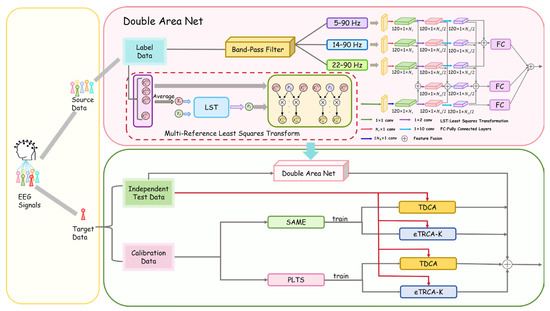
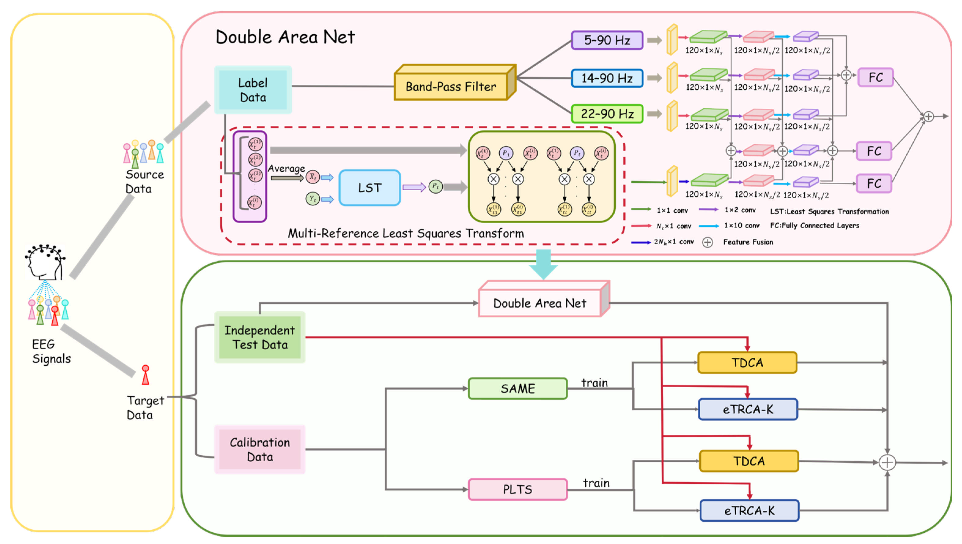
As shown in Figure 1, the proposed procedure consists of the following six steps:

Figure 1. Technical roadmap of the proposed method.

Step 1: Data Splitting. For dataset partitioning, a leave-one-subject-out cross-validation scheme is employed. Using the Benchmark dataset as an example, which includes 35 subjects, data from 34 subjects are used as the source-domain data in each iteration, while the remaining subject serves as the target-domain data. This procedure is repeated 35 times to ensure that every subject is used exactly once as the target-domain subject.

Step 2: Training the Double-Area network using source-domain data. The Double-Area network is designed to exploit the complementary characteristics of SSVEP representations, including multi-band harmonic information and stimulus-related periodic and phase-locked characteristics. Accordingly, the input EEG is processed through two parallel pathways with different representation mechanisms.

The first pathway is the Filter Path. SSVEP responses contain discriminative information not only at the fundamental stimulus frequency but also at multiple harmonic frequencies, and the relative strengths of these components may vary across participants and data lengths. Therefore, using only a single frequency band may not sufficiently exploit the complementary harmonic information. To address this issue, the Filter Path decomposes the EEG signals into three overlapping frequency bands (5–90 Hz, 14–90 Hz, and 22–90 Hz). The 5–90 Hz band preserves the fundamental and broad harmonic components, whereas the 14–90 Hz and 22–90 Hz bands progressively emphasize higher-frequency harmonic information. This hierarchical filter-bank design enables the network to learn complementary representations from different harmonic ranges rather than treating the entire spectrum uniformly.

After bandpass filtering, spatial features are extracted using 120 convolution kernels with size of Nc × 1, where Nc denotes the number of EEG channels. Subsequently, convolutional layers with kernel sizes 1 × 2 and 1 × 10 are applied to capture temporal-scale features, and the feature representations from the different sub-bands are then fused. The kernel size Nc × 1 indicates that spatial filtering is performed across all EEG channels, while the 1 × 2 and 1 × 10 kernels represent temporal convolution operations with different receptive fields. The number of convolution kernels (120) denotes the number of feature maps generated in each convolutional layer.

The second pathway is the Multi-Reference Least-Squares (MRLS) Path. Unlike the Filter Path, which learns data-driven representations from multiple harmonic bands, the MRLS Path incorporates prior knowledge of the periodic and phase-locked properties of SSVEP signals. Because SSVEP responses are synchronized with the visual stimulation, class-specific sine–cosine templates provide explicit references for the expected periodic response patterns. The MRLS transformation maps the EEG signals into this stimulus-related reference space through least-squares fitting, thereby emphasizing components consistent with the stimulus frequency and phase while reducing the influence of unrelated background activity. This reference-guided linear representation complements the nonlinear features learned by the Filter Path and provides additional stability when only limited calibration data are available.

The least-squares transform is a commonly used statistical method that constructs a linear relationship model between variables. Its primary objective is to estimate the parameters of the regression model by minimizing the sum of squared residuals, thereby quantifying the discrepancy between predicted values and actual observations. When $X$ and $Y$ represent two two-dimensional variables, the goal of the least-squares transform is to determine a transformation matrix $P$ by solving Equation (1):

$$\underset{P}{argmin}\parallel Y-PX{\displaystyle {\parallel }_F^2}$$

(1)

The solution to Equation (1) can be obtained using Equation (2):

$$P=Y{X}^T{(X{X}^T)}^{-1}$$

(2)

In this study, the Multi-Reference Least-Squares Transform is applied to each trial corresponding to each stimulus to generate a new multi-channel signal. Let ${\displaystyle X_t^{(i)}}\in R^{N_c\times N_s}$ denote the i-th trial of the t stimulus (corresponding to the i-th block of data for the t-th character), and let $Y_t$ represent the sine–cosine template associated with the stimulus frequency of the t-th stimulus. The objective of the MRLS Transform (MRLST) is to map the SSVEP signals from different subjects onto the sine–cosine template using Equation (3).

$$\underset{P_t}{\arg \min }\parallel Y_t-P_t{\overline{X}}_t{\displaystyle {\parallel }_F^2}$$

(3)

${\overline{X}}_t$ represents the average signal across all trials of the t-th stimulus. The sine–cosine template $Y_t$ corresponding to the t-th stimulus can be obtained using Equation (4).

$$Y_t=\left[\begin{array}{l}\hspace{1em}sin(2p{f}_t+f_t)\\ \hspace{1em}cos(2p{f}_t+f_t)\\ \hspace{1em}\hspace{1em} \dots \\ sin(2N_{h}p{f}_t+N_h{f}_t)\\ cos(2N_{h}p{f}_t+N_h{f}_t)\end{array}\right],t=[{\displaystyle \frac{1}{f_s}},{\displaystyle \frac{2}{f_s}},\dots {\displaystyle \frac{N_s}{f_s}}]$$

(4)

Here, $N_h$ denotes the number of harmonics (dimensionless), $f_t$ denotes the frequency of the t-th stimulus (Hz), ${\varphi }_t$ denotes the stimulus phase (rad), $N_s$ denotes the number of sampling points (points), and $f_s$ denotes the sampling rate (Hz). Once $P_t$ is obtained, the transformation is applied to each trial signal $X_t^{(i)}$ under each stimulus frequency to generate new data, as shown in Equation (5).

$$X_{tt}^{(i)}=P_t\times X_t^{(i)}$$

(5)

For example, in the Benchmark dataset, where there are 40 stimulus classes, 40 corresponding sine–cosine templates are constructed. The data processed by the MRLST are then passed through a convolutional layer with kernel size 1 × 1 for initial feature extraction, followed by a convolutional layer with 120 kernels (size = 2N_h × 1) to extract spatial information across channels, and finally through convolutional layers with 120 kernels of size 1 × 2 and 1 × 10 to capture temporal-scale features. To better leverage the information from both the filter path and the MRLS path, this study fuses the outputs of the first, second, and third convolutional layers from the Filter Path with the outputs of the second, third, and fourth convolutional layers from the MRLS path, and applies an additional convolution to the fused features. Ultimately, the outputs from the two paths are fed into fully connected layers for classification, and the final prediction is obtained by computing a weighted sum of their classification scores.

Step 3: Target-Domain Data Partitioning and Labeled-Data Augmentation. The target-domain data of each subject are first divided into Calibration data and Independent Test data. For each stimulus class, only one sample is selected as Calibration data, while all remaining samples are treated as Independent Test data (for example, in the Benchmark target-domain dataset, each class contains 1 Calibration sample and 5 Test samples). This process is iterated six times to perform cross-validation, ensuring that each sample serves as Calibration data exactly once. The Calibration data are then augmented using the SAME augmentation and PLTS augmentation methods. The detailed procedure is as follows:

(1)

SAME Augmentation

For the Calibration sample $X_t$ of a given stimulus class and the corresponding sine–cosine template $Y_t$ (with t denoting the stimulus class), the transformation matrix $\Phi$ is estimated by minimizing the mean squared error, as shown in Equation (6):

$$\hat{\Phi }=\underset{\Phi }{argmin}\parallel X_t-F{Y}_t{\parallel }_{\Phi }^2$$

(6)

where $\parallel {\parallel }_{\mathrm{F}}$ denotes the Frobenius norm. The solution to Equation (6) can be obtained by solving a least-squares problem The artificially reconstructed template signal ${\widehat{S}}_t$ is defined in Equation (7):

$${\widehat{S}}_t=\widehat{\Phi }{Y}_t$$

(7)

To generate multiple augmented signals, random noise is added to $\widehat{{\mathrm{S}}_{\mathrm{t}}}$. To ensure that the noise intensity added to each channel is proportional to the signal strength of $\widehat{{\mathrm{S}}_{\mathrm{t}}}$, let $s^c\in R^{1\times N_p}$ denote the signal of the c channel of $\widehat{{\mathrm{S}}_{\mathrm{t}}}$ and $\mathrm{D}({\mathit{s}}^{\mathrm{c}})$ denote the variance of the c-th channel signal. The covariance matrix of the noise $\Sigma \in R^{N_c\times N_c}$ can then be computed as shown in Equation (8):

$$\Sigma =diag(D(s^1),D(s^2),\dots ,D(s^{N_c}))$$

(8)

where diag( ) denotes arranging the elements along the diagonal, and Nc represents the number of channels. Finally, the artificially generated signals are produced according to Equation (9):

$${\displaystyle Z_t^{(k)}}={\stackrel{\wedge }{S}}_t+\alpha {\displaystyle W_{noise}^{(k)}},k=1,2,\dots N_a$$

(9)

$N_a$ denotes the number of generated signals. The generated ${\displaystyle W_{noise}^{(k)}}$ follow a Gaussian distribution [17] with a zero mean vector and a covariance matrix $\Sigma$, ${\displaystyle W_{noise}^{(k)}}~N(0,\Sigma )$. The parameter $\alpha$ is used to control the noise intensity and is set to 0.05.

(2)

PLTS Augmentation

To fully exploit the experimental data, in addition to the original samples ${\mathit{x}}_0[d,d+T_w]$ (extracted from time d with a duration of $T_w$ seconds), we assume that the data within each trial’s temporal window $[d+T_w,T_n]$ (where $T_n$ denotes the end time of the trial) can also be used for training the SSVEP model. Since subjects continuously fixate on the flickering stimulus throughout the entire trial, SSVEP responses are persistently elicited during this period. Specifically, the data extracted from any sub-interval $[a_t,a_t+T_w]$ (where $a_t$ denotes the starting point and $a_t+T_w$ denotes the ending point for generating new samples) within the trial should exhibit similar SSVEP characteristics with ${\mathit{x}}_0$ and can therefore serve as additional training samples. The optimal sub-interval for generating new data ${\mathit{x}}_a$ can be determined by locating the sampling point a that yields the maximum similarity, as defined in Equation (10).

$$a=argmax Similarity(x_0,x_a)$$

(10)

The similarity is measured by the correlation between $x_0$ and $x_a$, as defined in Equation (11).

$$Similarity(x_0,x_a)={\displaystyle \frac{\frac{{\displaystyle {\displaystyle {\sum }_{i=1}^{N_s}}(x_0[i]-\overline{x_0})(x_a[i]-\overline{x_a})}}{N-1}}{\sqrt{\frac{{\displaystyle {\displaystyle {\sum }_{i=1}^{N_s}}{(x_0[i]-\overline{x_0})}^2}}{N_s-1}+\epsilon }\sqrt{\frac{{\displaystyle {\displaystyle {\sum }_{i=1}^{N_s}}{(x_a[i]-\overline{x_a})}^2}}{N_s-1}+\epsilon }}}$$

(11)

Here, $\overline{x_0}$ and $\overline{x_a}$ denote the mean values of $x_0$ and $x_a$, respectively, and $N_s$ represents the number of selected data points (points). A small positive constant $\epsilon ={10}^{-8}$ is added to each variance term in the denominator to avoid division by zero when either input signal has zero or extremely small variance. Using a grid-search strategy, the starting point a is iteratively assigned values from the range $d\times f_s+1, d\times f_s+2, \dots , (T_n-T_w)\times f_s$. For each candidate a, the similarity between ${\mathit{x}}_0$ and ${\mathit{x}}_a$ is computed, and the sampling position that yields the highest similarity is chosen as the optimal a.

Based on SSVEP, the similarity between newly extracted samples $x_a$ and the original data $x_0$ exhibits a periodic pattern as the sampling position a varies, and this period equals the reciprocal of the stimulus frequency of the trial [17]. Therefore, for the n class of trial data (with a stimulus frequency of $f_n$ Hz), in addition to the original samples, time-shift-based augmentation can be employed to generate additional samples. The step size for this augmentation $\Delta s_n$ is computed as shown in Equation (12).

$$\Delta s_n={\displaystyle \frac{f_s}{f_n}}$$

(12)

The newly generated samples extracted within the interval of $[a_t,a_t+T_w]$ seconds can thus be used as additional training data. Accordingly, the sampling positions a are computed as defined in Equation (13).

$$a=a_t\times f_s=p\times \Delta s_n,p=1, 2, \dots , N_a$$

(13)

Here, $N_a$ denotes the number of generated signals.

Step 4: The datasets enhanced by the different methods are then separately used to train the eTRCA-K and TDCA models.

(1)

The training procedure of eTRCA-K is generally consistent with that of TRCA and it yields the average signal $\overline{{\mathit{X}}_t}\in R^{N_c\times N_s}(t=1, \dots , N_f)$ for each stimulus class. The main difference is that eTRCA-K integrates multiple spatial filters trained by TRCA into $\mathit{W}\in R^{N_c\times N_f}$, and employs Kendall correlation analysis instead of canonical correlation analysis for classification.

(2)

The training process of the TDCA model follows the description in reference [7]. After TDCA training, the optimal template parameter Q and the center $\overline{{\mathrm{A}}_{\mathrm{t}}}$ for each stimulus frequency are obtained.

Step 5: Classification of the Test Data. For the test data, classification is performed through five pathways: the trained Double-Area fusion network, SAME + eTRCA-K, SAME + TDCA, PLTS + eTRCA-K, and PLTS + TDCA. The classification procedures of eTRCA-K and TDCA are described as follows:

(1)

eTRCA-K

The correlation coefficient between the test data $x\in R^{N_c\times N_{\mathrm{s}}}$ and the average training signal $\overline{{\mathit{X}}_t}\in R^{N_c\times N_s}(t=1, \dots , N_f)$ of each class is computed as defined in Equation (14).

$${\lambda }_t=\varphi ({\mathit{W}}^{T}x,{\mathit{W}}^T{\overline{\mathit{X}}}_t), t=1, 2, \dots , N_f$$

(14)

Here, $\varphi (. , .)$ denotes the two-dimensional correlation analysis between the two signals, where the Kendall rank correlation coefficient is used.

(2)

TDCA

For the test data $x\in R^{N_c\times N_{\mathrm{s}}}$, the Pearson correlation coefficient between the sample and the class-specific center $\overline{A_{\mathrm{t}}}$ is computed, as given in Equation (15).

$$r_t=corr({\mathrm{Q}}^T{\stackrel{-}{\mathit{A}}}_t,{\mathit{Q}}^{T}x)$$

(15)

Step 6: Fusion and Classification of the Five Pathways. Let the feature vector of the k-th pathway be $y_k=[y_k(1),y_k(2),\dots \dots y_k(40)]$, where k = 1, 2, …5 corresponding to the outputs of the Double-Area network, SAME + eTRCA-K, SAME + TDCA, PLTS + eTRCA-K, and PLTS + TDCA, respectively. The fusion of the five pathways proceeds as follows: each output $y_k$ is first linearly normalized, as defined in Equation (16).

$${\displaystyle {\widehat{y}}_k^{(t)}}={\displaystyle \frac{y_k(t)-min(y_k)}{max(y_k)-min(y_k)+\epsilon }}$$

(16)

Here, $min(y_k)$ and $max(y_k)$ denote the minimum and maximum values of ${\mathrm{y}}_{\mathrm{k}}$, respectively, and t represents the t-th stimulus class. A small positive constant $\epsilon ={10}^{-8}$ is used to avoid division by zero when either input signal has zero or extremely small variance. The normalized feature vectors from the five pathways are then fused, as defined in Equation (17).

$$S(t)={\displaystyle {\displaystyle \sum _{k=1}^5}{\displaystyle {\widehat{y}}_k^{(t)}}}$$

(17)

The class t corresponding to the maximum value of $S\left(t\right)$ is identified as the predicted class of the test sample. Following score normalization, the group-balanced fusion ensures comparable contributions from the different pathways without introducing additional learnable parameters.

2.5. Evaluation Metrics and Baseline Methods

(1)

Evaluation Metrics

In this study, the performance of SSVEP recognition is evaluated primarily using two metrics: classification accuracy and ITR. Accuracy (ACC) represents the percentage of correctly identified stimulus classes relative to the total number of stimuli. ITR is the most commonly used performance metric in SSVEP, and is computed as shown in Equation (18).

$$ITR(bits/min)=(lo{g}_{2}N+plo{g}_{2}p+(1-p)lo{g}_2{\displaystyle \frac{1-p}{N-1}}){\displaystyle \frac{60}{T}}$$

(18)

In the formula, N denotes the number of stimulus frequencies, P is the average classification accuracy, and T is the average time (in seconds) required for recognition. In this study, the average time T includes a gaze shift interval of 0.5 s.

(2)

Baseline Methods

To evaluate the performance of the proposed method, it is compared with seven state-of-the-art SSVEP decoding algorithms: msCCA [5], FBCCA [2], TRCA [4], LST [20], Compact CNN [21], Ensemble DNN [22], and OS-SSVEP [15].

2.6. Experimental Settings

All experiments were conducted on a computer equipped with an AMD Ryzen 7 5800H CPU, 16 GB of system memory, and an NVIDIA GeForce RTX 3050 Laptop GPU with 4 GB of video memory. The operating system was 64-bit Windows 10. The software environment consisted of Python 3.10.0, PyTorch 1.12.1, CUDA 11.3, and cuDNN 8.3.2. Deep learning models were evaluated in FP32 on the GPU, whereas the conventional matrix-based methods were executed on the CPU.

(1)

Computational Complexity Analysis

As shown in Table 1, the proposed method contains 0.642 M trainable parameters and requires 108.866 M neural-branch FLOPs per trial. Its standardized fitting/training time and inference latency were 0.921 s and 356.377 ms per trial, respectively, which were higher than those of OS-SSVEP (0.527 s and 177.235 ms). This additional cost mainly arises from combining the complementary SAME and PLTS decision pathways. Nevertheless, the inference latency remained below the 0.5-s EEG acquisition window, and the proposed method required substantially fewer stored parameters than Ensemble DNN (0.642 M versus 15.881 M). Together with the numerically highest classification accuracy at all six data lengths, these results indicate that the proposed method favors decoding performance and complementary feature utilization rather than minimum computational cost, yielding a modest but consistent performance improvement at the expense of additional inference time.

Table 1. Computational complexity comparison of the proposed method and baseline methods on the Benchmark dataset.

Method Names	Parameters (M)	FLOPs (M/Trial)	Timed Fitting/Training (s)	Inference (ms/Trial)	Peak Training Memory (MB)
msCCA	N/A	N/A	0.371	26.649	384.32
FBCCA	N/A	N/A	<0.001	40.022	0.001
TRCA	N/A	N/A	0.13	58.703	2.428
LST	N/A	N/A	0.013	5.237	0.059
CompactCNN	0.055	81.78	0.216	0.595	1565.461
Ensemble DNN	15.881	22.063 × k	1.921	0.941 × k	20.814
OS-SSVEP	0.642	108.866	0.527	177.235	79.688
Ours	0.642	108.866	0.921	356.377	79.688

Note: N/A indicates that parameter count and neural network FLOPs are not applicable to conventional methods without trainable neural networks. The reported fitting/training time represents a standardized profiling workload rather than complete training to convergence. k denotes the number of dynamically activated constituent networks in Ensemble DNN.

(2)

Sensitivity analysis

A preliminary local sensitivity analysis was conducted on the Benchmark dataset using data lengths of 0.5, 0.8, and 1.0 s. In the sensitivity analysis, the noise-intensity coefficient was varied among 0.03, 0.05, and 0.07; the number of SAME-generated samples among 1, 3, and 5; and the number of PLTS-generated samples among 4, 6, and 8. The default settings were a SAME noise-intensity coefficient of 0.05, three SAME-generated samples, and six PLTS-generated samples. Only one parameter was varied at a time, while the remaining parameters were fixed at their default values. The same trained model, data partition, and random seed were maintained across all configurations. The observed within-condition performance variations were 1.50, 0.50, and 0.50 percentage points for data lengths of 0.5, 0.8, and 1.0 s, respectively. Thus, the maximum variation did not exceed 1.50 percentage points, indicating that the proposed framework was relatively stable within the evaluated parameter ranges.

3. Results

3.1. Comparison Between the Proposed Model and State-of-the-Art Methods

As shown in Table 2, for the Benchmark dataset, at data lengths of 0.5–0.6 s, the classification accuracy ranks from highest to lowest as follows: the proposed method, OS-SSVEP, TRCA, Ensemble DNN, msCCA, LST, Compact CNN, and FBCCA; at data lengths of 0.7–0.9 s, the ranking is as follows: the proposed method, OS-SSVEP, TRCA, Ensemble DNN, LST, msCCA, Compact CNN, and FBCCA; at a data length of 1 s, the ranking is as follows: the proposed method, OS-SSVEP, TRCA, LST, Ensemble DNN, msCCA, FBCCA, and Compact CNN. The proposed method achieves the highest ACC on the Benchmark dataset, and all other methods are significantly different from it across all data lengths.

Table 2. Comparison of the ACC (%) on the Benchmark dataset.

Method Categories	Method Names	Data Lengths (s)
		0.5 s	0.6 s	0.7 s	0.8 s	0.9 s	1.0 s
Traditional Methods	msCCA	50.13 ± 3.74 *	56.60 ± 3.89 *	63.95 ± 3.95 *	70.19 ± 3.75 *	74.58 ± 3.64 *	77.89 ± 3.49 *
	FBCCA	20.9 ± 1.94 *	30.6 ± 2.72 *	41.1 ± 3.37 *	49.50 ± 3.58 *	58.3 ± 3.68 *	65.6 ± 3.72 *
	TRCA	62.3 ± 3.73 *	70.7 ± 3.67 *	81.2 ± 2.88 *	83.57 ± 3.12 *	86.95 ± 2.83 *	89.04 ± 2.63 *
	LST	43.22 ± 3.68 *	53.25 ± 3.92 *	64.93 ± 3.99 *	74.04 ± 3.92 *	76.69 ± 3.65 *	83.18 ± 3.42 *
Deep Learning Methods	Compact CNN	33.65 ± 2.94 *	40.70 ± 3.35 *	48.69 ± 3.50 *	56.15 ± 3.56 *	59.99 ± 3.61 *	64.63 ± 3.55 *
	Ensemble Dnn	53.92 ± 3.87 *	61.78 ± 3.82 *	69.01 ± 3.81 *	74.40 ± 3.72 *	78.62 ± 3.61 *	80.88 ± 3.53 *
	OS-SSVEP	76.53 ± 3.05 *	82.65 ± 2.78 *	87.45 ± 2.55 *	90.55 ± 2.19 *	92.79 ± 1.84 *	94.05 ± 1.59 *
	Ours	78.91 ± 2.89	84.22 ± 2.57	88.60 ± 2.32	91.50 ± 2.03	93.29 ± 1.73	94.39 ± 1.53

Note: Boldface indicates the best performance. The asterisks indicate statistically significant differences from the proposed method: * (p < 0.001).

As shown in Table 3, for the Benchmark dataset, at data lengths of 0.5–0.6 s, the ITR ranks from highest to lowest as follows: the proposed method, OS-SSVEP, TRCA, Ensemble DNN, msCCA, LST, Compact CNN, and FBCCA; at 0.7 s, the ranking is as follows: the proposed method, OS-SSVEP, TRCA, Ensemble DNN, LST, msCCA, Compact CNN, and FBCCA; at 0.8–0.9 s, the ranking is as follows: the proposed method, OS-SSVEP, TRCA, LST, Ensemble DNN, msCCA, Compact CNN, and FBCCA; at 1 s, the ranking is as follows: the proposed method, OS-SSVEP, TRCA, LST, Ensemble DNN, msCCA, FBCCA, and Compact CNN. These results indicate that the proposed method achieves the highest accuracy and ITR across all data lengths. A similar pattern is observed for ITR; the proposed method obtains the highest ITR on the Benchmark dataset.

Table 3. Comparison of ITR (bits/min) on the Benchmark dataset.

Method Categories	Method Names	Data Lengths (s)
		0.5 s	0.6 s	0.7 s	0.8 s	0.9 s	1.0 s
Traditional Methods	msCCA	110.79 ± 11.96 *	120.86 ± 11.78 *	133.09 ± 11.47 *	140.60 ± 10.39 *	143.13 ± 9.65 *	142.64 ± 8.80 *
	FBCCA	27.48 ± 4.28 *	48.78 ± 6.70 *	67.83 ± 8.15 *	82.58 ± 8.70 *	98.04 ± 8.83 *	109.49 ± 8.84 *
	TRCA	152.70 ± 12.92 *	168.10 ± 12.10 *	188.08 ± 9.58 *	183.23 ± 9.34 *	180.83 ± 8.13 *	175.28 ± 7.23 *
	LST	89.65 ± 11.07 *	111.01 ± 11.55 *	136.65 ± 11.47 *	153.94 ± 10.85 *	159.52 ± 9.85 *	159.0 ± 8.96 *
Deep Learning Methods	Compact CNN	59.79 ± 8.01 *	73.04 ± 9.08 *	87.33 ± 9.26 *	99.59 ± 9.13 *	102.27 ± 8.72 *	106.5 ± 8.23 *
	Ensemble Dnn	123.28 ± 12.82 *	136.84 ± 12.11 *	148.35 ± 11.47 *	153.28 ± 10.65 *	155.51 ± 10.01 *	151.68 ± 9.27 *
	OS-SSVEP	205.63 ± 11.64 *	210.82 ± 10.13 *	211.83 ± 8.83 *	206.77 ± 7.35 *	199.65 ± 5.99 *	190.50 ± 5.03 *
	Ours	215.15 ± 11.18	216.65 ± 9.59	215.80 ± 8.24	210.11 ± 6.94	201.30 ± 5.73	191.59 ± 4.86

Note: Boldface indicates the best performance. The asterisks indicate statistically significant differences from the proposed method: * (p < 0.001).

3.2. Effect of Data Length on Different Models

(1)

Comparison of Models at Different Data Lengths

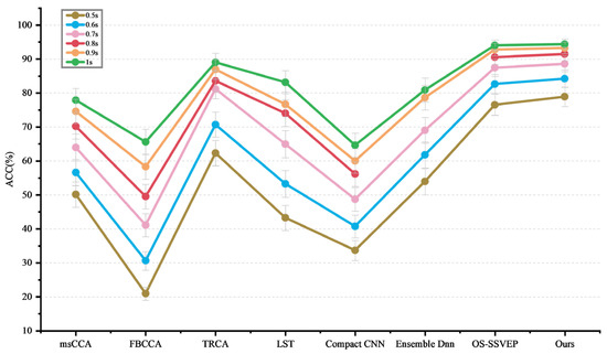
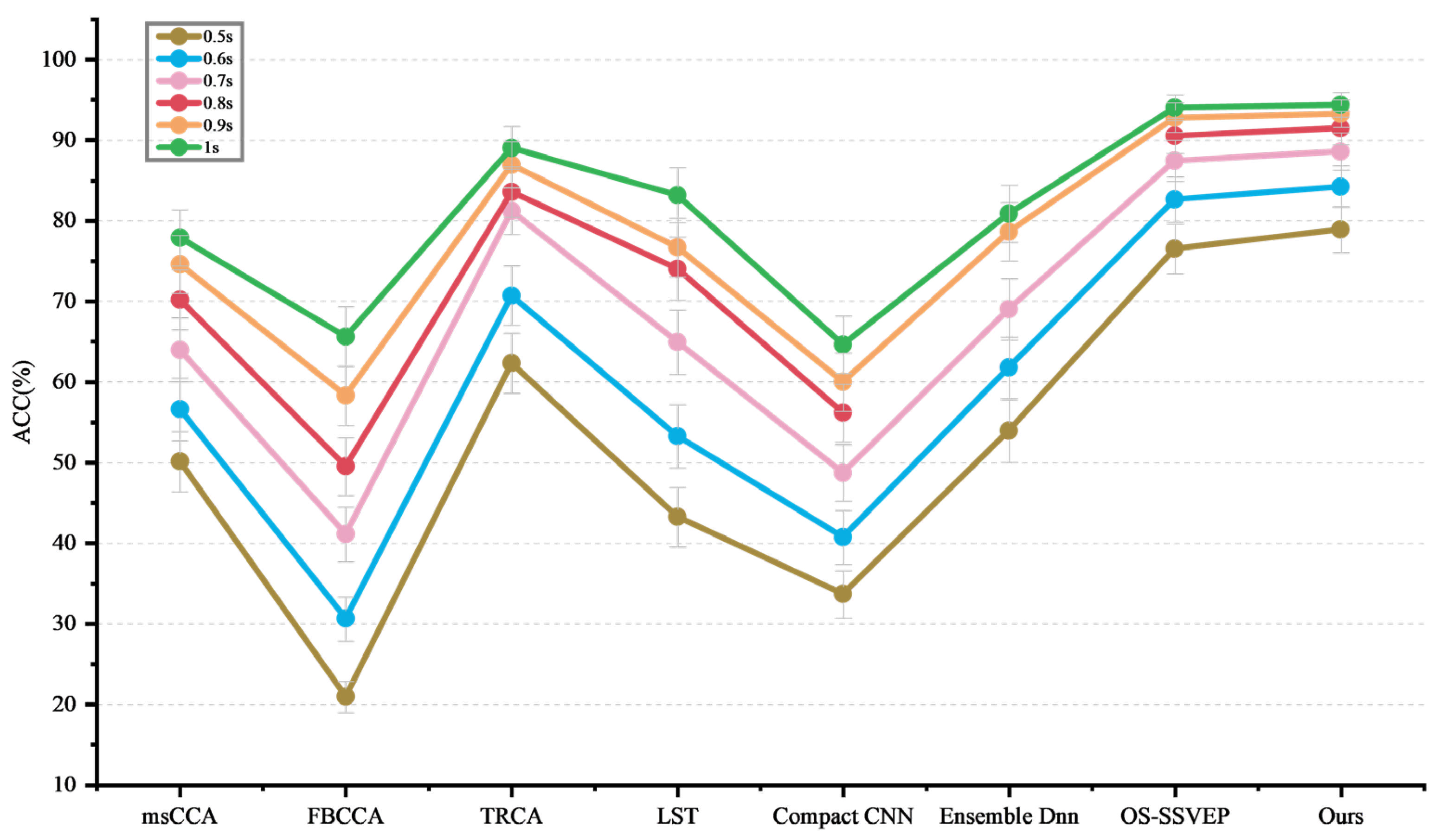
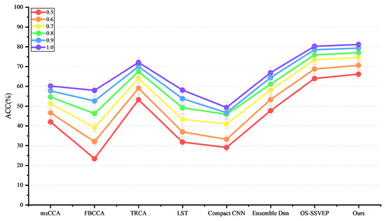
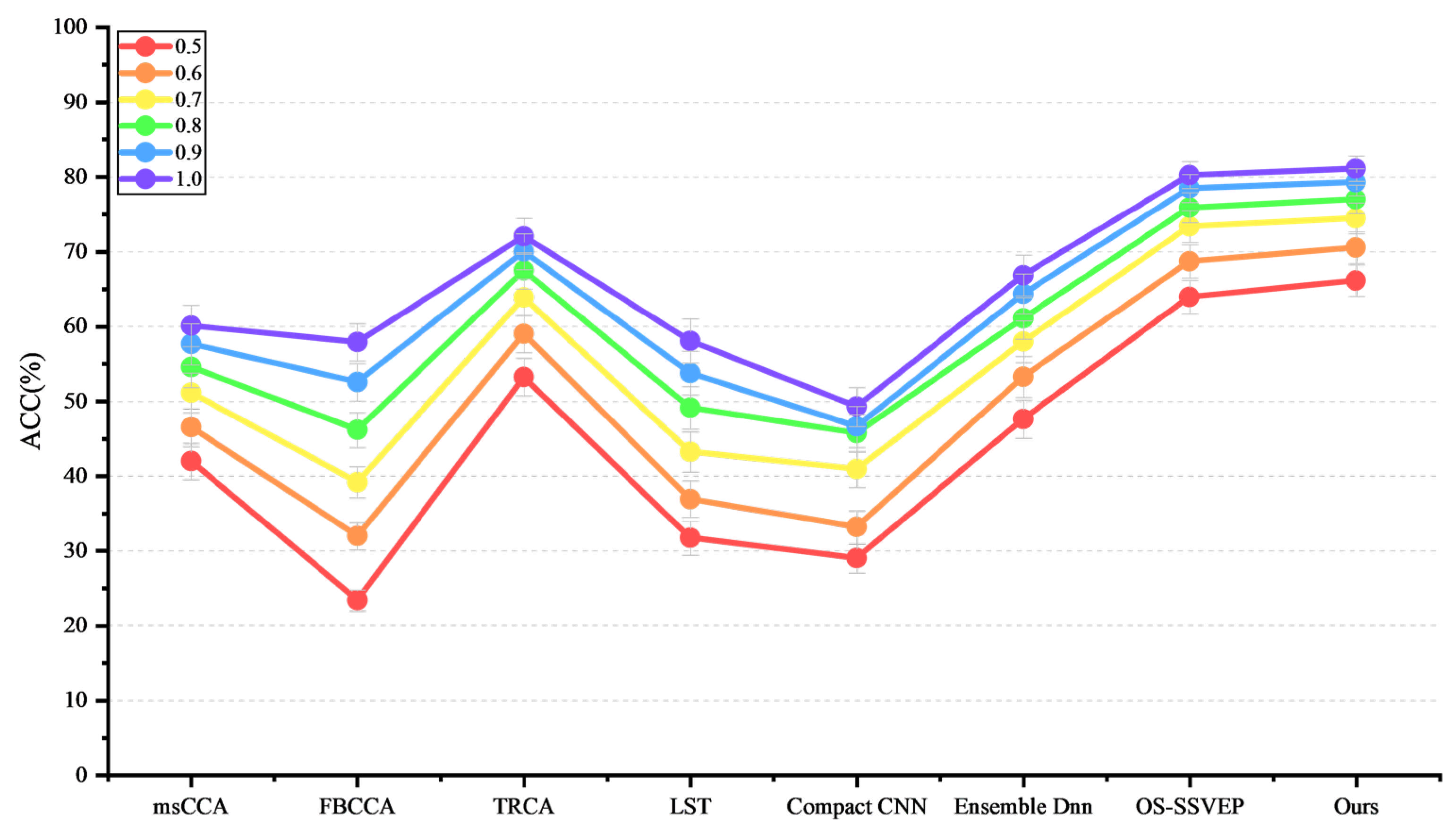
As shown in Figure 2, for all methods, classification accuracy increases with data length, which is consistent with the decoding characteristics of SSVEP. For the Benchmark dataset, considering the concentration of accuracy values over the range of 0.5–1 s, the proposed method exhibits the most concentrated accuracy across all data lengths, followed by OS-SSVEP, while FBCCA performs the worst. Furthermore, the difference in accuracy between the 1 s and 0.5 s data from largest to smallest is as follows: FBCCA (44.7), LST (39.96), Compact CNN (30.98), msCCA (27.76), TRCA (26.74), Ensemble DNN (26.29), OS-SSVEP (17.52), and the proposed method (15.48). This demonstrates that the impact of data length on the accuracy of the proposed method is minimal.

Figure 2. Comparison of the ACC (%) of different methods on the Benchmark dataset.

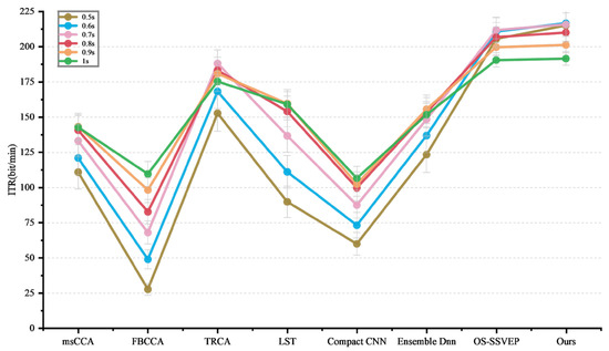
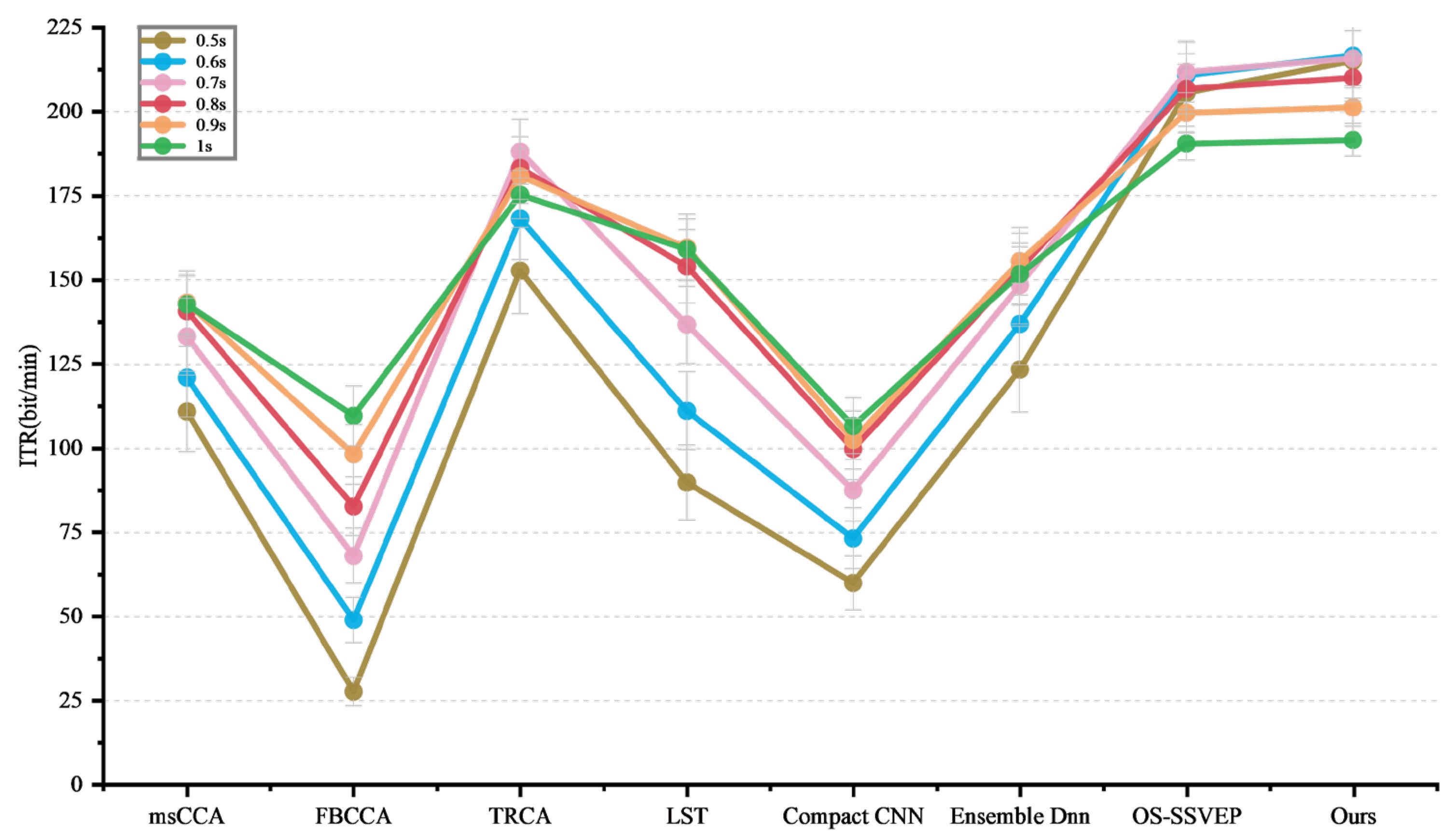
As shown in Table 3, for all methods, the ITR generally increases and then decreases with data length (although this trend is not fully observed for some methods within the 0.5–1 s range), which is consistent with the periodic steady-state characteristics of SSVEP responses. For the Benchmark dataset, as illustrated in Figure 3, the data lengths at which the maximum ITR is achieved for the proposed method, OS-SSVEP, TRCA, Ensemble DNN, LST, msCCA, FBCCA, and Compact CNN are 0.6 s, 0.7 s, 0.7 s, 0.9 s, 0.9 s, 0.9 s, 1 s, and 1 s, respectively. These results indicate that the proposed method reaches the highest ITR in the shortest time, followed by OS-SSVEP and TRCA, then Ensemble DNN, LST, and msCCA, and finally FBCCA and Compact CNN.

Figure 3. Comparison of ITR (bits/min) achieved by different methods on the Benchmark dataset.

(2)

Comparison of Single-Branch Pathways at Different Data Lengths

As shown in Table 4, the proposed method clearly outperforms single-pathway classification. On the Benchmark dataset, the relative importance of the five pathways varies across different data lengths. At 0.5 s and 0.6 s, the classification accuracy ranks from highest to lowest as follows: Double-Area network, TDCA with PLTS, TDCA with SAME, eTRCA-K with PLTS, and eTRCA-K with SAME; at 0.7 s: Double-Area network, TDCA with SAME, TDCA with PLTS, eTRCA-K with PLTS, and eTRCA-K with SAME; at 0.8 s: TDCA with SAME, TDCA with PLTS, eTRCA-K with SAME, Double-Area network, and eTRCA-K with PLTS; at 0.9 s: TDCA with SAME, TDCA with PLTS, Double-Area network, eTRCA-K with SAME, and eTRCA-K with PLTS; at 1.0 s: TDCA with SAME, TDCA with PLTS, eTRCA-K with SAME, Double-Area network, and eTRCA-K with PLTS. These results indicate that different pathways are suited to different data lengths. For shorter data segments, the Double-Area network contributes more significantly to decoding, whereas for longer segments, the importance of SAME-based augmentation becomes more pronounced. Overall, TDCA exhibits substantially better classification performance than eTRCA-K. The proposed method significantly outperforms every single-branch pathway in ACC across all data lengths on the Benchmark dataset.

Table 4. ACC (%) of different single-branch pathways on the Benchmark dataset.

Methods	Data Lengths (s)
	0.5 s	0.6 s	0.7 s	0.8 s	0.9 s	1.0 s
DoubleArea	70.82 ± 3.05 *	76.38 ± 2.97 *	81.23 ± 2.88 *	85.35 ± 2.72 *	87.05 ± 2.57 *	88.44 ± 2.50 *
eTRCA-K with SAME	62.30 ± 3.74 *	70.74 ± 3.67 *	78.18 ± 3.42 *	83.57 ± 3.13 *	86.95 ± 2.83 *	89.04 ± 2.64 *
TDCA with SAME	64.82 ± 3.73 *	73.42 ± 3.71 *	80.32 ± 3.42 *	85.41 ± 3.02 *	88.82 ± 2.61 *	91.11 ± 2.32 *
eTRCA-K with PLTS	64.80 ± 3.54 *	71.85 ± 3.48 *	78.37 ± 3.24 *	83.07 ± 2.97 *	86.10 ± 2.72 *	88.15 ± 2.53 *
TDCA with PLTS	66.30 ± 3.39 *	73.44 ± 3.28 *	80.31 ± 3.01 *	84.89 ± 2.73 *	87.90 ± 2.48 *	89.89 ± 2.26 *
Ours	78.91 ± 2.89	84.22 ± 2.57	88.60 ± 2.32	91.50 ± 2.03	93.29 ± 1.73	94.39 ± 1.53

Note: Boldface indicates the best performance. The asterisks indicate statistically significant differences from the proposed method: * (p < 0.001).

As shown in Table 5, the ITR achieved by the proposed method is clearly superior to that of single-pathway classification. On the Benchmark dataset, the relative importance of the five pathways varies with data length. At 0.5 s and 0.6 s, the ITR ranks from highest to lowest as follows: Double-Area network, TDCA + PLTS, TDCA + SAME, eTRCA-K + PLTS, and eTRCA-K + SAME; at 0.7 s: Double-Area network, TDCA + SAME, TDCA + PLTS, eTRCA-K + PLTS, and eTRCA-K + SAME; at 0.8 s: TDCA + SAME, TDCA + PLTS, eTRCA-K + SAME, Double-Area network, and eTRCA-K + PLTS; at 0.9 s: TDCA + SAME, TDCA + PLTS, Double-Area network, eTRCA-K + SAME, and eTRCA-K + PLTS; at 1.0 s: TDCA + SAME, TDCA + PLTS, eTRCA-K + SAME, Double-Area network, and eTRCA-K + PLTS. These results indicate that different pathways are suitable for different data lengths. For shorter data segments, the Double-Area network achieves better decoding performance, whereas for longer segments, decoding performance after SAME-based augmentation is superior. Overall, TDCA exhibits significantly better classification performance than eTRCA-K. The proposed method significantly improves ITR over all single-branch pathways across all data lengths, confirming the effectiveness of multi-pathway fusion.

Table 5. ITR (bits/min) of different single-branch pathways on the Benchmark dataset.

Methods	Data Lengths (s)
	0.5 s	0.6 s	0.7 s	0.8 s	0.9 s	1.0 s
DoubleArea	181.63 ± 11.26 *	185.89 ± 10.41 *	188.08 ± 9.58 *	188.14 ± 8.64 *	180.25 ± 7.73 *	172.76 ± 7.10 *
eTRCA-K with SAME	152.70 ± 12.92 *	168.10 ± 12.10 *	179.17 ± 10.72 *	183.23 ± 9.34 *	180.83 ± 8.13 *	175.28 ± 7.23 *
TDCA with SAME	161.28 ± 12.96 *	177.21 ± 12.15 *	186.24 ± 10.81 *	189.13 ± 9.26 *	186.51 ± 7.79 *	181.2 ± 6.59 *
eTRCA-K with PLTS	160.97 ± 12.27 *	171.01 ± 11.51 *	178.90 ± 10.28 *	180.65 ± 9.00 *	177.41 ± 7.92 *	171.90 ± 7.06 *
TDCA with PLTS	165.55 ± 11.82 *	175.91 ± 10.88 *	185.06 ± 9.68 *	186.29 ± 8.42 *	182.88 ± 7.36 *	176.92 ± 6.43 *
Ours	215.15 ± 11.18	216.65 ± 9.59	215.80 ± 8.24	210.11 ± 6.94	201.30 ± 5.73	191.59 ± 4.86

Note: Boldface indicates the best performance. The asterisks indicate statistically significant differences from the proposed method: * (p < 0.001).

3.3. Robustness of the Proposed Method Across Datasets

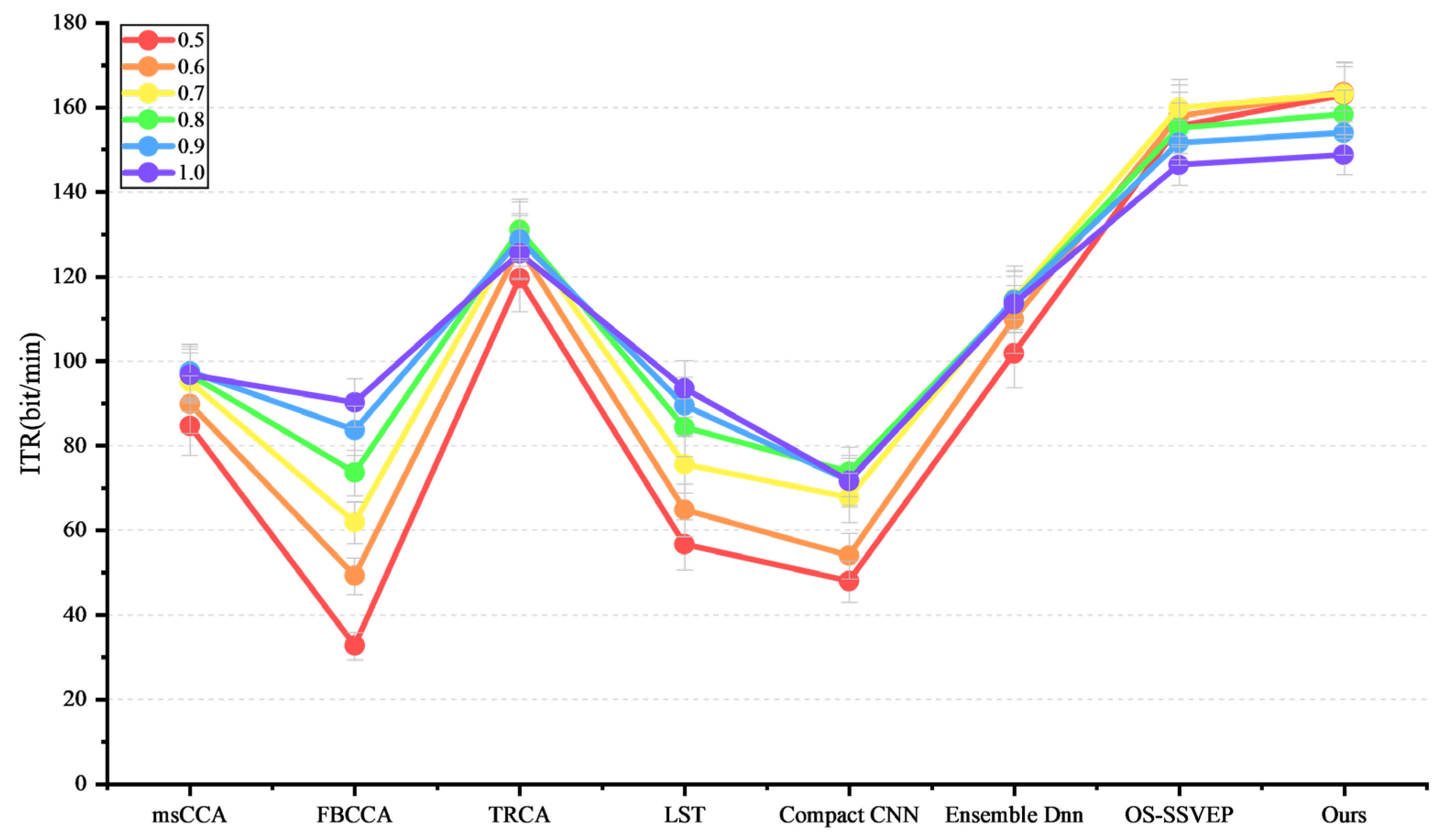
For the BETA dataset, as shown in Table 6 and Table 7, the proposed method achieves the highest classification accuracy and ITR across data lengths from 0.5 s to 1 s. As illustrated in Figure 4 and Figure 5, the impact of data length on SSVEP decoding is minimal for the proposed method (with the most concentrated results, see Figure 4), and the shortest data length required to achieve the optimal ITR is 0.6 s (see Figure 5). On the BETA dataset, the proposed method achieves the highest ACC and ITR across all data lengths, with significant differences from all baseline methods.

Table 6. Comparison of the ACC (%) achieved by different methods on the BETA dataset.

Method Categories	Method Names	Data Lengths (s)
		0.5 s	0.6 s	0.7 s	0.8 s	0.9 s	1.0 s
Traditional Methods	msCCA	41.96 ± 2.42 *	46.51 ± 2.54 *	51.12 ± 2.68 *	54.57 ± 2.73 *	57.65 ± 2.76 *	60.09 ± 2.76 *
	FBCCA	23.37 ± 1.41 *	31.96 ± 1.82 *	39.14 ± 2.08 *	46.15 ± 2.30 *	52.55 ± 2.50 *	57.88 ± 2.51 *
	TRCA	53.22 ± 2.49 *	59.01 ± 2.53 *	63.88 ± 2.52 *	67.48 ± 2.43 *	70.03 ± 2.39 *	72.05 ± 2.38 *
	LST	31.69 ± 2.23 *	36.88 ± 2.45 *	43.20 ± 2.70 *	49.11 ± 2.87 *	53.76 ± 2.91 *	58.05 ± 2.96 *
Deep Learning Methods	Compact CNN	28.98 ± 1.96 *	33.13 ± 2.22 *	40.89 ± 2.42 *	45.71 ± 2.52 *	46.60 ± 2.77 *	49.25 ± 2.60 *
	Ensemble Dnn	47.61 ± 2.55 *	53.26 ± 2.70 *	57.95 ± 2.80 *	61.07 ± 2.73 *	64.35 ± 2.68 *	66.83 ± 2.75 *
	OS-SSVEP	63.94 ± 2.27 *	68.72 ± 2.24 *	73.38 ± 2.12 *	75.88 ± 2.00 *	78.49 ± 1.87 *	80.26 ± 1.77 *
	Ours	66.13 ± 2.13	70.55 ± 2.10	74.46 ± 2.04	77.00 ± 1.91	79.32 ± 1.81	81.11 ± 1.72

Note: Boldface indicates the best performance. The asterisks indicate statistically significant differences from the proposed method: * (p < 0.001).

Table 7. Comparison of the ITR (bits/min) achieved by different methods on the BETA dataset.

Method Categories	Method Names	Data Lengths (s)
		0.5 s	0.6 s	0.7 s	0.8 s	0.9 s	1.0 s
Traditional Methods	msCCA	84.60 ± 6.83 *	89.79 ± 6.78 *	95.04 ± 6.92 *	96.74 ± 6.70 *	97.49 ± 6.52 *	96.72 ± 6.17 *
	FBCCA	32.57 ± 3.27 *	49.16 ± 4.34 *	61.77 ± 4.97 *	73.57 ± 5.42 *	83.60 ± 5.80 *	90.14 ± 5.71 *
	TRCA	119.51 ± 7.80 *	126.85 ± 7.56 *	131.07 ± 7.24 *	131.00 ± 6.63 *	128.68 ± 6.20 *	125.50 ± 5.83 *
	LST	56.55 ± 5.94 *	64.74 ± 6.21 *	75.49 ± 6.71 *	84.28 ± 6.90 *	89.43 ± 6.75 *	93.48 ± 6.57 *
Deep Learning Methods	Compact CNN	47.85 ± 4.90 *	53.92 ± 5.39 *	67.69 ± 5.83 *	73.75 ± 5.87 *	71.62 ± 6.15 *	71.54 ± 5.59 *
	Ensemble Dnn	101.76 ± 8.06 *	109.89 ± 8.02 *	114.65 ± 7.89 *	114.10 ± 7.36 *	114.37 ± 6.89 *	113.51 ± 6.71 *
	OS-SSVEP	155.59 ± 7.96 *	157.98 ± 7.34 *	159.89 ± 6.66 *	155.14 ± 5.97 *	151.62 ± 5.33 *	146.40 ± 4.80 *
	Ours	162.99 ± 7.59	163.68 ± 7.02	163.22 ± 6.50	158.40 ± 5.77	153.99 ± 5.24	148.77 ± 4.72

Note: Boldface indicates the best performance. The asterisks indicate statistically significant differences from the proposed method: * (p < 0.001).

Figure 4. Comparison of ACC (%) of 8 different methods on the BETA dataset.

Figure 5. Comparison of ITR (bits/min) of 8 different methods on the BETA dataset.

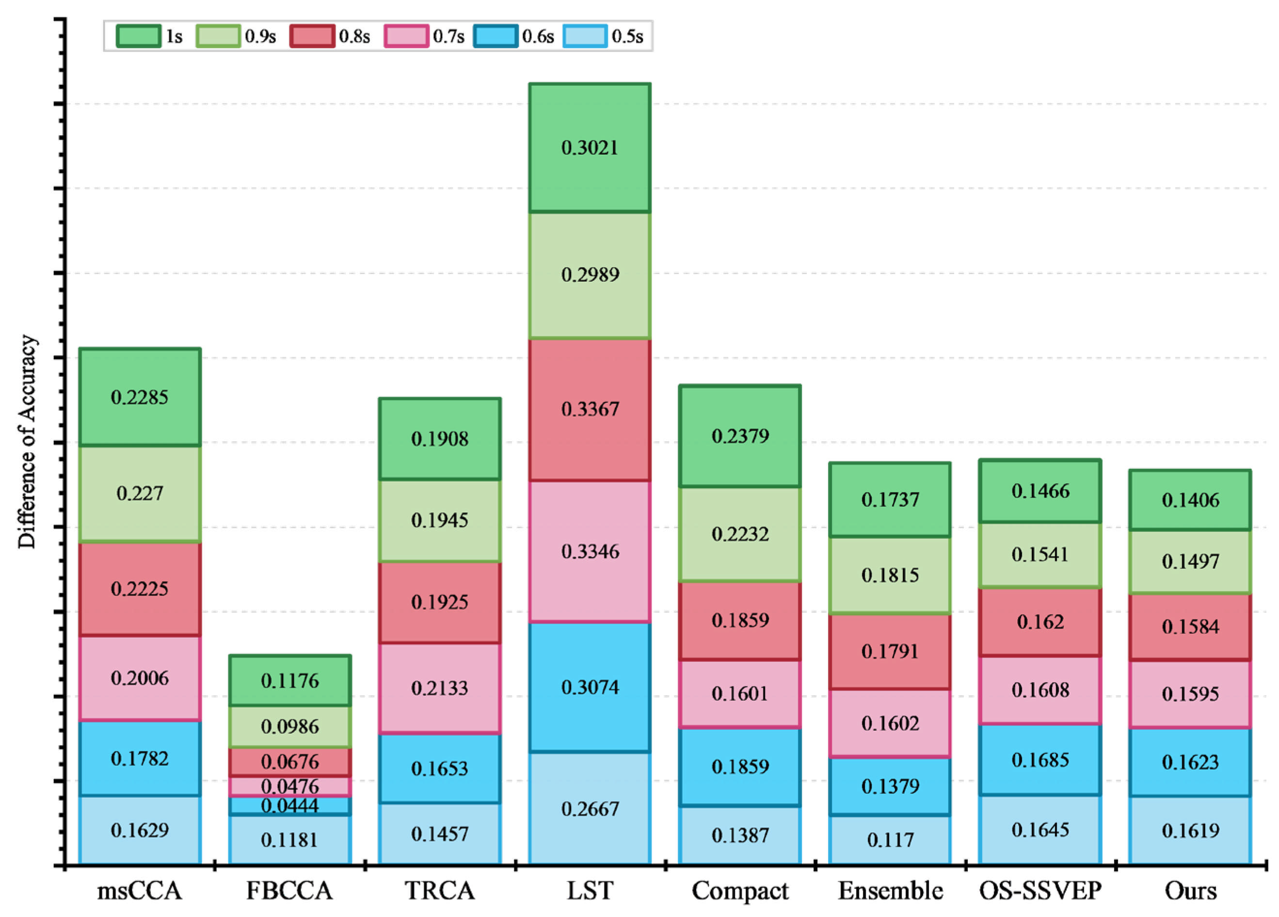
As shown in Figure 6, for the proposed method, the difference in decoding accuracy (Benchmark-Beat/Benchmark) between the two datasets at data lengths of 0.5 s, 0.6 s, 0.7 s, 0.8 s, 0.9 s, and 1 s is 16.19%, 16.23%, 15.95%, 15.84%, 14.97%, and 14.06%, respectively. For OS-SSVEP, the corresponding differences are 16.45%, 16.85%, 16.08%, 16.20%, 15.41%, and 14.66%; for Ensemble DNN: 11.70%, 13.79%, 16.02%, 17.91%, 18.15%, and 17.37%; for Compact CNN: 13.87%, 18.59%, 16.01%, 18.59%, 22.32%, and 23.79%; for LST: 26.67%, 30.74%, 33.46%, 33.67%, 29.89%, and 30.21%; for TRCA: 14.57%, 16.53%, 21.33%, 19.25%, 19.45%, and 19.08%; for FBCCA: 11.81%, 4.44%, 4.76%, 6.76%, 9.86%, and 11.76%; and for msCCA: 16.29%, 17.82%, 20.06%, 22.25%, 22.70%, and 22.85%. From these results, it can be observed that for data lengths greater than 0.7 s, the accuracy difference between the two datasets is the second smallest for the proposed method (the smallest is FBCCA, which has extremely low decoding accuracy and limited practical applicability). The same approach was applied to ITR calculation, yielding results consistent with the accuracy comparison, thereby demonstrating the robustness of the proposed method for cross-dataset SSVEP decoding.

Figure 6. Comparison of decoding accuracy across different data lengths on the Benchmark and BETA datasets.

3.4. Ablation Study

As shown in Table 8, on the Benchmark dataset, for longer data lengths (1 s), removing the Double-Area network module, eTRCA-K + SAME, eTRCA-K + PLTS, TDCA + SAME, and TDCA + PLTS resulted in a decrease in classification accuracy from 94.39% to 91.82% (−2.57%), 94.21% (−0.18%), 94.18% (−0.21%), 94.30% (−0.09%), and 94.27% (−0.12%), respectively. For shorter data lengths (e.g., 0.6 s), accuracy dropped from 84.22% to 77.41% (−6.81%), 83.84% (−0.39%), 83.92% (−0.30%), 84.07% (−0.15%), and 83.91% (−0.31%), indicating that the Double-Area network has the greatest impact on overall model performance, especially for shorter data lengths.

Table 8. ACC (%) in the ablation study on the Benchmark dataset.

Parameter Selections					Data Lengths (s)
Double-Area Network	eTRCA-K with SAME	eTRCA-K with PLTS	TDCA with SAME	TDCA with PLTS	0.6 s	0.7 s	0.8 s	0.9 s	1 s
×	√	√	√	√	77.41 ± 3.22	83.33 ± 2.94	87.45 ± 2.58	90.24 ± 2.28	91.82 ± 2.01
√	×	√	√	√	83.84 ± 2.62	88.34 ± 2.37	91.30 ± 2.08	93.06 ± 1.77	94.21 ± 1.56
√	√	×	√	√	83.92 ± 2.57	88.39 ± 2.32	91.35 ± 2.02	93.15 ± 1.75	94.18 ± 1.55
√	√	√	×	√	84.07 ± 2.61	88.36 ± 2.37	91.43 ± 2.06	93.29 ± 1.75	94.30 ± 1.53
√	√	√	√	×	83.91 ± 2.63	88.26 ± 2.37	91.31 ± 2.08	93.13 ± 1.75	94.27 ± 1.57
√	√	×	√	×	83.15 ± 2.75	87.58 ± 2.50	90.92 ± 2.17	92.84 ± 1.84	94.10 ± 1.61
√	×	√	×	√	82.93 ± 2.66	87.64 ± 2.38	90.74 ± 2.11	92.54 ± 1.83	93.71 ± 1.64
√	√	√	√	√	84.22 ± 2.57	88.60 ± 2.32	91.50 ± 2.03	93.28 ± 1.73	94.39 ± 1.53

Note: Boldface indicates the best performance. The cross (×) in the table represents the absence of this module, and the tick (√) represents the presence of this module.

From the perspective of data augmentation, removing PLTS-related modules (eTRCA-K + PLTS and TDCA + PLTS) led to a decrease in accuracy from 94.39% to 94.10% (−0.29%) at 1 s and from 84.22% to 83.15% (−1.07%) at 0.6 s. Removing SAME-related modules (eTRCA-K + SAME and TDCA + SAME) resulted in performance reductions from 94.39% to 93.71% (−0.68%) at 1 s and from 84.22% to 82.93% (−1.29%) at 0.6 s, suggesting that, among individual augmentation modules, SAME has a greater overall impact on model performance than PLTS.

The ITR results presented in Table 9 are consistent with those in Table 7 and are not repeated here.

Table 9. ITR (bits/min) in the ablation study on the Benchmark dataset.

Parameter Selections					Data Lengths (s)
Double-Area Network	eTRCA-K with SAME	eTRCA-K with PLTS	TDCA with SAME	TDCA with PLTS	0.6 s	0.7 s	0.8 s	0.9 s	1 s
×	√	√	√	√	191.12 ± 9.05	196.44 ± 9.61	195.54 ± 8.16	190.99 ± 6.97	183.15 ± 5.95
√	×	√	√	√	215.21 ± 9.74	214.87 ± 8.38	209.43 ± 7.06	200.53 ± 5.82	190.98 ± 4.93
√	√	×	√	√	215.37 ± 9.59	214.89 ± 8.23	209.46 ± 6.91	200.81 ± 5.76	190.88 ± 4.92
√	√	√	×	√	216.17 ± 9.70	214.95 ± 8.37	209.89 ± 7.00	201.37 ± 5.76	191.33 ± 4.85
√	√	√	√	×	215.56 ± 9.74	214.51 ± 8.37	209.48 ± 7.05	200.75 ± 5.77	191.28 ± 4.96
√	√	×	√	×	212.75 ± 9.37	212.12 ± 8.67	208.20 ± 7.30	199.83 ± 5.99	190.77 ± 5.07
√	×	√	×	√	211.45 ± 9.81	211.97 ± 8.41	207.25 ± 7.16	198.60 ± 5.97	189.30 ± 5.13
√	√	√	√	√	216.65 ± 9.60	215.80 ± 8.24	210.11 ± 6.93	201.30 ± 5.73	191.59 ± 4.86

Note: Boldface indicates the best performance. The cross (×) in the table represents the absence of this module, and the tick (√) represents the presence of this module.

4. Discussion

This study presents an elegant framework that integrates five SSVEP decoding pathways, each with distinct strengths and complementary advantages. The framework leverages the strengths of different pathways under varying data conditions (e.g., data length, signal-to-noise ratio) while mitigating their weaknesses, achieving high-performance, robust, and data-length-insensitive SSVEP decoding.

4.1. Advantages of the Proposed Method

The proposed method does not simply stack similar models; rather, it creatively fuses data-driven deep learning models (Double-Area network) with traditional discriminative models (eTRCA-K and TDCA). The Double-Area network comprises a Filter Path and a MRLS path. The Filter Path employs multiple parallel band-pass filters covering different frequency bands where SSVEP signals may occur, ensuring comprehensive extraction of frequency-domain features. The MRLS path directly uses sine–cosine templates as references for transformation, projecting the data toward ideal SSVEP response patterns and effectively highlighting phase-locked information related to the stimulus frequency. By fusing features from different layers of the two paths, the Double-Area network can simultaneously exploit low-level (detailed) and high-level (abstract) information, enriching the hierarchical representation of features. Consequently, the Double-Area network can automatically learn complex, high-level nonlinear features from raw data without relying on strong assumptions, offering greater adaptability. In contrast, TDCA and eTRCA-K are based on traditional signal correlation and spatial filtering techniques, with clear underlying principles, and are highly effective when the data meet their model assumptions. These two types of discriminative paradigms are fundamentally complementary: when one model underperforms due to specific data characteristics, the other can still provide stable performance, thereby ensuring the overall robustness of the system.

Of course, the high performance achieved in this study also relies on a dual-pronged data augmentation strategy. To address the critical issue of having very few calibration samples in the target domain, two augmentation methods are introduced. SAME augmentation effectively expands the training dataset by adding noise to the template signals that matches the channel signals, enhancing noise robustness and preventing the model from overfitting to the limited samples. PLTS augmentation cleverly exploits the periodic nature of SSVEP signals to generate multiple homologous training samples from a single trial. This not only increases the data volume but allows the model to learn the temporal dynamics and stability (sequential characteristics) of SSVEP signals, thereby enhancing temporal generalization capability.

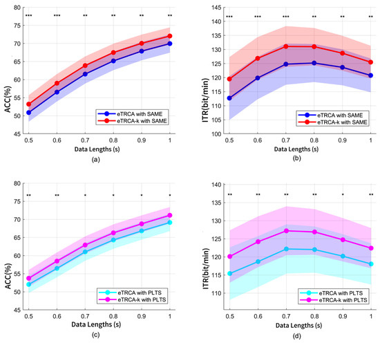
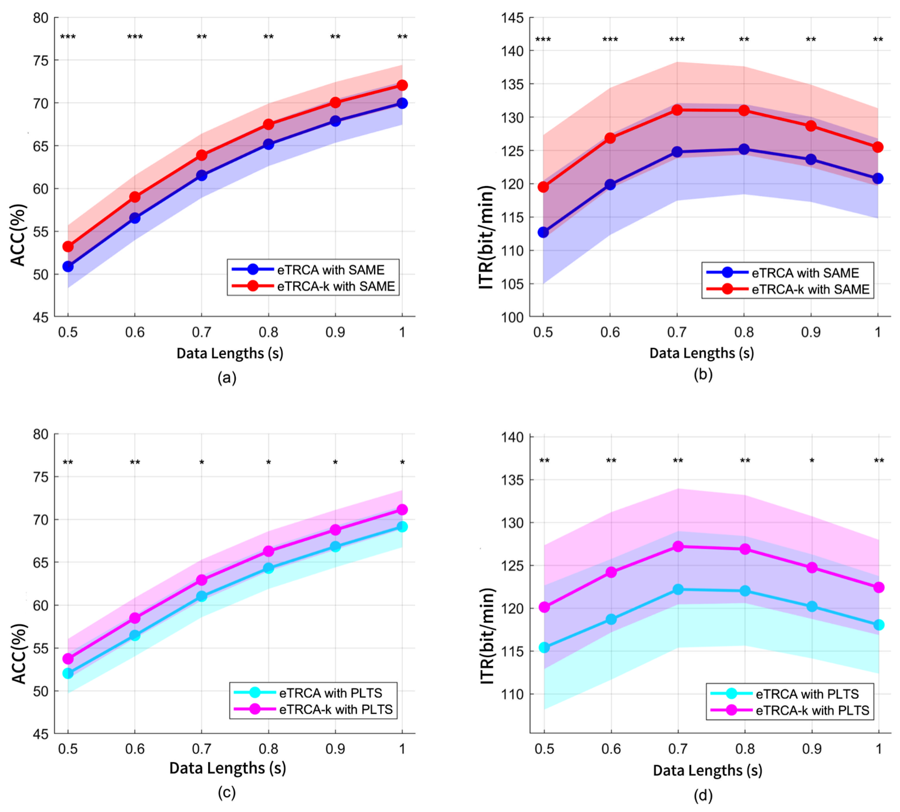
After applying SAME or PLTS augmentation, TDCA’s inter-class optimization strategy converts the supplemented temporal dynamic features into class-discriminative information, enabling the synergistic use of dynamic information and class boundaries, and addressing issues of insufficient feature dimensionality and class overlap. The eTRCA-K replaces the traditional correlation coefficient with Kendall correlation analysis, which is more sensitive to nonlinear temporal correlations. Compared with standard eTRCA, this modification leads to improved SSVEP decoding performance (see Figure 7).

Figure 7. Comparison of eTRCA and eTRCA-K. The shaded regions represent the standard deviation. The asterisks in the figure indicate significant differences determined by Paired T-tests (* denotes p < 0.05, ** denotes p < 0.01, *** denotes p < 0.001).

4.2. Impact of Data Length on SSVEP Decoding

One of the most prominent advantages of the proposed method is its insensitivity to data length, which mainly arises from the multi-level, multi-mechanism synergistic effect. First, the Double-Area network, trained end-to-end, can learn to extract highly discriminative micro-patterns or instantaneous phase features from limited data points, maintaining good performance even with short data segments. Within the Double-Area network, the MRLST transformation is based on least-squares fitting to the ideal template. Even with short data segments, as long as the basic response pattern is present, this transformation can effectively separate signal from noise and map it to the template space, providing fundamental stability.

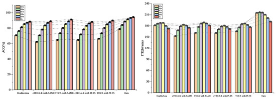
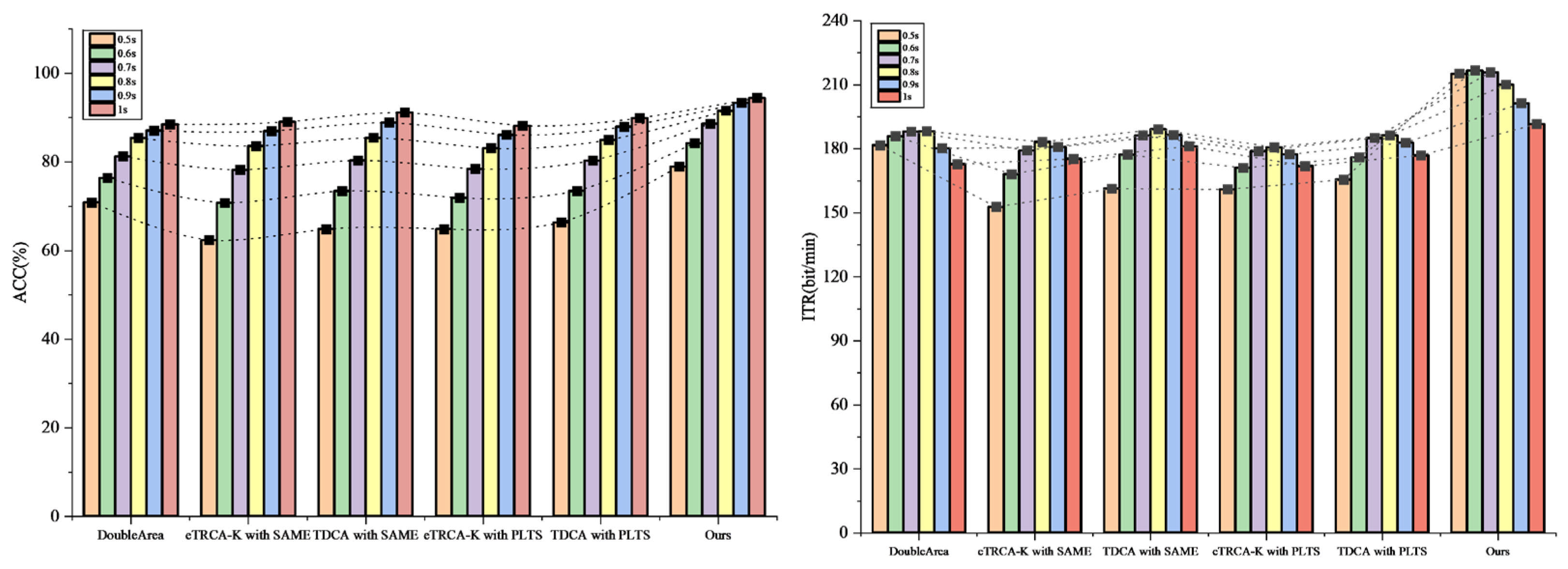
Secondly, methods such as eTRCA-K and TDCA rely on inter-signal correlations, and longer data provide more cycles and more stable statistical properties, making the computed signal templates and correlation measures more reliable, thereby significantly improving performance (as shown in Figure 8).

Figure 8. Classification ACC (%) and ITR (bits/min) achieved by single-branch pathways on the Benchmark dataset.

Thirdly, the SAME and PLTS augmentation strategies reduce interference from random neural activity. SAME first computes the average SSVEP template from the original calibration data and then estimates the mixing matrix based on this template. With medium- to long-length data, the template SNR is higher and the estimation error of the mixing matrix is smaller, allowing the generated artificial EEG signals to accurately match the frequency and phase characteristics of real SSVEP signals, avoiding feature distortion caused by cycle truncation. The main challenge with short- to medium-length data is the complex variation in temporal dynamics and lower robustness, coupled with insufficient individual specificity, which can lead to matching bias. PLTS extracts the time segments with the highest similarity via optimal temporal shifts, supplementing missing temporal dynamics in short- to medium-length data. The synergistic effect of SAME and PLTS thus reduces interference and enhances the feature representation used for classification.

4.3. Analysis of Model Robustness and Generalization

In terms of handling noise and data uncertainty, SAME augmentation introduces noise designed according to the channel variance, exposing the model to simulated realistic noise during training and thereby enhancing its robustness. From the perspective of multi-pathway fusion, even if one or several branches make incorrect predictions due to noise interference, the final fused output can still be correct as long as the other branches make accurate judgments. This greatly reduces the probability of failure caused by local issues.

Regarding information utilization, PLTS and SAME augmentation fully exploit the value of a very small amount of labeled data, mitigating overfitting in small-sample learning and ensuring that the model is adequately trained in the target domain. These factors collectively enable the proposed method to demonstrate stronger robustness when confronted with noise and uncertain data.

5. Limitations and Future Work

Although the proposed method was evaluated on the Benchmark and BETA datasets, both use closely related 40-target joint frequency-phase modulation paradigms. Therefore, the current results demonstrate robustness across participant cohorts and acquisition settings within similar paradigms, rather than broad generalization to substantially different BCI configurations. Moreover, phase coding was not treated as an independent experimental factor. Future studies will evaluate the framework using more diverse target numbers, controlled frequency-phase combinations, stimulation protocols, acquisition devices, and hybrid or multimodal paradigms.

The present evaluation was based on offline public datasets collected under controlled conditions and therefore did not capture motion artifacts, environmental noise, attention fluctuations, inter-session variability, or other challenges of online BCI operation. Under the one-shot Benchmark protocol, the experimental calibration procedure for each stimulus class requires approximately 6 s. Therefore, the total calibration time increases approximately linearly with the number of stimulus classes, reaching approximately 240 s (4 min) when all 40 classes are included. However, electrode preparation, subjective fatigue, visual discomfort, and user acceptance were not measured. Future work will conduct online and session-level usability evaluations incorporating these practical factors.

Finally, the five-path ensemble introduces additional computational cost, while the SAME and PLTS augmentation parameters are manually specified and the current group-balanced fusion uses fixed weights. Although this parameter-free fusion reduces the risk of overfitting under one-shot calibration, it cannot adapt to variations in pathway reliability across participants, trials, or data lengths. Future work will investigate lightweight inference, data-driven augmentation-parameter selection, and confidence-aware or data-length-dependent fusion using an independent validation protocol to avoid overfitting and test-data leakage.

6. Conclusions

In this study, we proposed an individual-adapted SSVEP decoding framework that integrates hybrid data augmentation, collaborative discrimination, and a Double-Area network to address the fundamental challenges of limited calibration data and substantial inter-subject variability in SSVEP-based BCI systems. Building upon a multi-path ensemble architecture, the proposed method incorporates SAME-based static feature augmentation and PLTS-based temporal-dynamic enhancement to enrich subject-specific calibration data, while eTRCA-K and TDCA are employed to strengthen feature extraction across individuals. In parallel, the Double-Area network introduces a complementary deep hierarchical representation that captures nonlinear spatiotemporal patterns and multi-harmonic structures crucial for SSVEP decoding. By jointly modeling subject-level adaptation, harmonic-sensitive feature learning, and pathway-level fusion, the proposed framework effectively mitigates the sensitivity of SSVEP decoding to data length and enhances both robustness and generalization across subjects and datasets. This design addresses the core challenges of data scarcity, individual variability, and temporal instability in SSVEP-based BCIs, enabling more accurate, reliable, and user-friendly target recognition for real-world BCI applications.

References

- Lin, Z.; Zhang, C.; Wu, W.; Gao, X. Frequency recognition based on canonical correlation analysis for SSVEP-based BCIs. IEEE Trans. Biomed. Eng. 2006, 53, 2610–2614. [Google Scholar] [CrossRef] [Scilit]
- Chen, X.; Wang, Y.; Gao, S.; Jung, T.-P.; Gao, X. Filter bank canonical correlation analysis for implementing a high-speed SSVEP-based brain–computer interface. J. Neural Eng. 2015, 12, 046008. [Google Scholar] [CrossRef] [Scilit]
- Zhang, Y.; Xia, M.; Chen, K.; Xu, P.; Yao, D. Progresses and prospects on frequency recognition methods for steady-state visual evoked potential. J. Biomed. Eng. 2022, 39, 192–197. [Google Scholar]
- Nakanishi, M.; Wang, Y.; Chen, X.; Wang, Y.-T.; Gao, X.; Jung, T.-P. Enhancing detection of SSVEPs for a high-speed brain speller using task-related component analysis. IEEE Trans. Biomed. Eng. 2017, 65, 104–112. [Google Scholar] [CrossRef] [Scilit]
- Wong, C.M.; Wan, F.; Wang, B.; Wang, Z.; Nan, W.; Lao, K.F.; Mak, P.U.; Vai, M.I.; Rosa, A. Learning across multi-stimulus enhances target recognition methods in SSVEP-based BCIs. J. Neural Eng. 2020, 17, 016026. [Google Scholar] [CrossRef] [Scilit]
- Xu, M.; Wu, Q.; Xiong, W.; Xiao, X.; Ming, D. Research on encoding and decoding algorithms for medium/high-frequency SSVEP-based brain-computer interface. J. Signal Process. 2022, 38, 1881–1891. [Google Scholar]
- Liu, B.; Chen, X.; Shi, N.; Wang, Y.; Gao, S.; Gao, X. Improving the performance of individually calibrated SSVEP-BCI by task-discriminant component analysis. IEEE Trans. Neural Syst. Rehabil. Eng. 2021, 29, 1998–2007. [Google Scholar] [CrossRef] [Scilit]
- Kwak, N.-S.; Müller, K.-R.; Lee, S.-W. A convolutional neural network for steady state visual evoked potential classification under ambulatory environment. PLoS ONE 2017, 12, e0172578. [Google Scholar] [CrossRef]
- Lawhern, V.J.; Solon, A.J.; Waytowich, N.R.; Gordon, S.M.; Hung, C.P.; Lance, B.J. EEGNet: A compact convolutional neural network for EEG-based brain–computer interfaces. J. Neural Eng. 2018, 15, 056013. [Google Scholar] [CrossRef] [Scilit] [PubMed]
- Waytowich, N.; Lawhern, V.J.; Garcia, J.O.; Cummings, J.; Faller, J.; Sajda, P.; Vettel, J.M. Compact convolutional neural networks for classification of asynchronous steady-state visual evoked potentials. J. Neural Eng. 2018, 15, 066031. [Google Scholar] [CrossRef] [Scilit]
- Guney, O.B.; Oblokulov, M.; Ozkan, H. A deep neural network for ssvep-based brain-computer interfaces. IEEE Trans. Biomed. Eng. 2021, 69, 932–944. [Google Scholar] [CrossRef] [Scilit]
- Pan, Y.; Chen, J.; Zhang, Y.; Zhang, Y. An efficient CNN-LSTM network with spectral normalization and label smoothing technologies for SSVEP frequency recognition. J. Neural Eng. 2022, 19, 056014. [Google Scholar] [CrossRef] [Scilit]
- Deng, Y.; Sun, Q.; Wang, C.; Wang, Y.; Zhou, S.K. TRCA-Net: Using TRCA filters to boost the SSVEP classification with convolutional neural network. J. Neural Eng. 2023, 20, 046005. [Google Scholar] [CrossRef] [Scilit]
- Li, D.; Huang, Y.; Luo, R.; Zhao, L.; Xiao, X.; Wang, K.; Yi, W.; Xu, M.; Ming, D. Enhancing detection of SSVEPs using discriminant compacted network. J. Neural Eng. 2025, 22, 016043. [Google Scholar] [CrossRef] [Scilit]
- Deng, Y.; Ji, Z.; Wang, Y.; Zhou, S.K. OS-SSVEP: One-shot SSVEP classification. Neural Netw. 2024, 180, 106734. [Google Scholar] [CrossRef] [Scilit]
- Luo, R.; Xu, M.; Zhou, X.; Xiao, X.; Jung, T.-P.; Ming, D. Data augmentation of SSVEPs using source aliasing matrix estimation for brain–computer interfaces. IEEE Trans. Biomed. Eng. 2022, 70, 1775–1785. [Google Scholar] [CrossRef] [Scilit]
- Mai, X.; Ai, J.; Wei, Y.; Zhu, X.; Meng, J. Phase-locked time-shift data augmentation method for SSVEP brain-computer interfaces. IEEE Trans. Neural Syst. Rehabil. Eng. 2023, 31, 4096–4105. [Google Scholar] [CrossRef] [Scilit]
- Wang, Y.; Chen, X.; Gao, X.; Gao, S. A benchmark dataset for SSVEP-based brain–computer interfaces. IEEE Trans. Neural Syst. Rehabil. Eng. 2016, 25, 1746–1752. [Google Scholar] [CrossRef] [Scilit]
- Liu, B.; Huang, X.; Wang, Y.; Chen, X.; Gao, X. BETA: A Large Benchmark Database Toward SSVEP-BCI Application. Front. Neurosci. 2020, 14, 627. [Google Scholar] [CrossRef] [Scilit]
- Bian, R.; Wu, H.; Liu, B.; Wu, D. Small data least-squares transformation (sd-LST) for fast calibration of SSVEP-based BCIs. IEEE Trans. Neural Syst. Rehabil. Eng. 2022, 31, 446–455. [Google Scholar] [CrossRef] [Scilit]
- Convolutions, C.-W. Channelnets: Compact and efficient convolutional neural networks via. IEEE Trans. Pattern Anal. Mach. Intell. 2021, 43, 2570–2581. [Google Scholar] [CrossRef] [Scilit]
- Guney, O.B.; Ozkan, H. Transfer learning of an ensemble of DNNs for SSVEP BCI spellers without user-specific training. J. Neural Eng. 2023, 20, 016013. [Google Scholar] [CrossRef] [Scilit]
Disclaimer/Publisher’s Note: The statements, opinions and data contained in all publications are solely those of the individual author(s) and contributor(s) and not of MDPI and/or the editor(s). MDPI and/or the editor(s) disclaim responsibility for any injury to people or property resulting from any ideas, methods, instructions or products referred to in the content. |
© 2026 by the authors. Licensee MDPI, Basel, Switzerland. This article is an open access article distributed under the terms and conditions of the Creative Commons Attribution (CC BY) license.