


Abstract
(1) Background: Phishing remains a pervasive and economically damaging cyberthreat. The dominant detection paradigm has moved toward deep neural and transformer-based classifiers, a literature that reports high accuracy and that does not, in general, expose a per-decision justification, whereas interpretability and auditability are increasingly required in regulated environments; no comparison against transformer-scale detectors is made in this paper. This work asks how far a fully interpretable detector can close the accuracy gap to an opaque text classifier while preserving per-decision explanations, and what such a detector returns that accuracy alone does not measure. (2) Methods: HIEF, an interpretable evidence-fusion framework, is presented. Each email is represented by eighteen human-readable signals: fourteen structural and linguistic cues and four lexical aggregates derived from a published sparse log-odds lexicon. The signals are fused by three transparent layers, namely an -regularized logistic model, a shallow interaction-rule tree, and a calibrated Dempster–Shafer stage that reports belief, disbelief and ignorance masses together with an order-invariant global conflict coefficient derived in closed form. A logistic meta-learner fitted on out-of-fold component scores integrates the three layers. The evidential layer uses a type-aware calibration in which discrete signals are calibrated on their attainable values and continuous signals by isotonic regression. Evaluation uses 38,908 public emails, 38,512 of them after exact-duplicate removal, with near-duplicate control, group-aware partitioning, ten repeated splits, a source-held-out protocol, a two-class cross-source test set, a component ablation and a human audit of 100 messages annotated independently by two evaluators. (3) Results: Under group-aware partitioning, HIEF attains an of 0.855 and the strongest term frequency–inverse document frequency (TF–IDF) baseline 0.954; a compact character n-gram neural reference model, evaluated over the same ten partitions, attains 0.973. The linear layer alone attains 0.872, so the two fusion layers do not improve accuracy over it, and the paired difference of 0.017 excludes zero. Type-aware calibration raises the evidential layer from 0.771 to 0.780 and more than halves its partition-to-partition standard deviation, but does not make it competitive; the weakness, therefore, lies in the fusion formulation rather than in the binning. What the evidential layer does supply is a decomposable account of decision uncertainty: the ignorance mass separates errors from correct decisions, 0.265 against 0.175. The human audit reaches an inter-annotator Cohen’s kappa of 0.950 over the five categories before adjudication, and shows that the permissive corpus label agrees with human phishing judgment at a Cohen’s kappa between 0.18 and 0.21, against 0.70 to 0.77 for the automatic strict rule; the audited block is annotated by two of the authors and its human positives are confined to the advance-fee family, so the audit is a bounded comparison of label assignments and not an independent annotation study. (4) Conclusions: HIEF is positioned as an uncertainty and explanation framework rather than as an accuracy-improving fusion method, since the measured accuracy cost of the fusion layers is not compensated by an accuracy gain. Quantifying how much of the performance reported on these widely used corpora is attributable to template leakage and to label permissiveness is a contribution independent of the detector itself. Cross-source operation has not been demonstrated: specificity falls to 0.041 on an unseen collection, so all evaluation reported here is proof-of-concept and no operational deployment claim is made. The Spanish-language evaluation rests on a small and entirely positive subset and is reported as preliminary.
1. Introduction
Phishing is a social-engineering attack delivered predominantly through electronic mail, in which an adversary impersonates a trusted entity to induce a victim to disclose confidential information or to execute malicious content. Unlike attacks that exploit software vulnerabilities, phishing targets human cognition and, therefore, does not require advanced technical capability on the part of the attacker, which makes it both highly accessible and difficult to eliminate [1,2]. The scale of the problem has grown sharply: annual phishing reports remained below 200,000 from 2013 through 2019, surpassed 500,000 by the end of 2020, and exceeded 1.5 million by 2023 [3].
The associated economic impact is severe. The Verizon Data Breach Investigations Report attributes the large majority of confirmed breaches to a human element, of which phishing is the dominant vector [4]. The IBM/Ponemon Cost of a Data Breach Report places the global average cost of a breach in 2022 at USD 4.35 million [5], and the Internet Crime Complaint Center of the Federal Bureau of Investigation reports adjusted losses from business email compromise in the billions of dollars for the same period [6]. The three quantities are cited separately because each comes from a different source.
Contemporary mail providers filter the overwhelming majority of malicious messages. The operator of the largest consumer mail service reports that its automated defenses stop more than 99.9 percent of spam, phishing and malware, corresponding to nearly fifteen billion unwanted messages per day [7]. This is a vendor-reported operational statistic rather than an independently audited measurement, and it is used here only to motivate the existence of a residual risk surface. The residual fraction that evades filtering reaches end users without any accompanying indication of risk. This observation motivates a complementary line of defense: lightweight, on-device or gateway-level detectors that not only classify a message but also communicate why it was flagged. In high-stakes or regulated environments, the ability to justify an automated security decision in human-readable terms is increasingly a governance requirement rather than a design preference. An opaque classifier that emits only a probability provides no basis for an analyst to audit, contest, or learn from its output.
Phishing is not a monolithic phenomenon, and the heterogeneity of its subtypes is part of what makes detection difficult. Mass-distributed campaigns cast a wide net with generic lures, whereas spear-phishing targets specific individuals with personalized context, and business-email-compromise attacks impersonate executives or vendors to authorize fraudulent transfers. Advance-fee fraud, of which the Nigerian-letter genre is the canonical example, relies on a narrative of unexpected wealth and urgency. These subtypes differ in their surface features. Some are lexically florid and easily separable, while others are terse and structurally indistinguishable from legitimate correspondence. A detector that depends on a single class of signal will, therefore, perform unevenly across subtypes. Part of the design rationale adopted here is that fusing heterogeneous signals provides robustness across this spectrum. Transparent fusion additionally allows an analyst to see which subtype a given decision corresponds to.
The dominant research trend has moved in the opposite direction. State-of-the-art phishing detectors increasingly rely on deep neural architectures and large pre-trained language models that achieve excellent benchmark accuracy at the cost of interpretability, substantial computational demand, and a dependence on large labeled corpora [8,9]. This creates a practical tension. On one hand, simple text classifiers built on term-frequency representations already attain near-perfect benchmark scores. On the other hand, neither these nor their deep-learning successors expose the reasoning behind an individual decision.
This work addresses two questions. The first is how far can a fully interpretable detector close the accuracy gap to an opaque text classifier, while preserving per-decision explanations? The second follows from the answer to the first: if the interpretable detector does not win on accuracy, what does it return that an accuracy comparison does not measure? Both questions are answered with HIEF, an interpretable evidence-fusion framework. The central design principle adopted here is that interpretability and competitive accuracy are not mutually exclusive if (i) hand-engineered signals are augmented with a small and auditable lexical representation rather than a high-dimensional opaque one, and (ii) these signals are combined through fusion operators that are themselves transparent and that explicitly represent uncertainty. The evidence reported below supports the first half of that principle and not the second: the compact lexical representation buys accuracy, whereas the two fusion layers do not. HIEF is, therefore, presented as an uncertainty and explanation framework, and the accuracy of its linear layer is reported as the operative accuracy of the approach.
A second contribution is reported here as a finding of equal standing, and it concerns the benchmark rather than the detector. The public corpora on which phishing detectors are conventionally benchmarked contain large families of templated campaigns, forwarded threads and mailing-list traffic, and their distributed labels pool unsolicited commercial mail with credential phishing. When a message and its near-duplicate fall on opposite sides of a stratified split, the resulting scores measure memorization of templates rather than detection of phishing. Template leakage is quantified here at 0.084 points for the interpretable detector and 0.034 for the strongest opaque baseline. A human audit of 100 messages, annotated independently by two evaluators, further shows that the distributed label agrees with human phishing judgment at a Cohen’s kappa between 0.18 and 0.21. Because an auditable lexicon makes the responsible tokens visible, an interpretable detector is a usable instrument for diagnosing both problems, and it is usable for that purpose whether or not it wins an accuracy comparison.
The contributions of this paper are the following:
- The arbitrary, hand-assigned weights of a conventional heuristic phishing scorer are replaced by statistically learned weights obtained from an -regularized logistic model. The fitted model yields sparse, sign-interpretable coefficients with bootstrap confidence intervals.
- A compact, published lexical representation is introduced: four human-readable aggregate features computed from a sparse log-odds lexicon. These features recover a substantial part of the discriminative power of a 20,000-dimensional term frequency–inverse document frequency (TF–IDF) vector while remaining fully auditable token by token.
- Phishing detection is formulated as an evidence-fusion problem, and a calibrated, continuous Dempster–Shafer stage is developed under a type-aware calibration in which discrete signals are calibrated on their attainable values and continuous signals by isotonic regression. A global conflict coefficient is derived in closed form; it is provably invariant to the order in which sources are combined, whereas the pairwise-sum measure used in earlier formulations is not (Proposition 1).
- The two fusion layers are evaluated against the linear layer on quantities other than , namely the decomposition of decision uncertainty into an ignorance mass and a conflict mass, the separation of those quantities between correct and incorrect decisions, and selective risk under a coverage constraint. The accuracy comparison and the uncertainty comparison are reported together, including where the fusion layers lose.
- The validity of the benchmark itself is quantified: the contribution of template leakage to reported performance, the contribution of corpus-exclusive vocabulary, the collapse of specificity under a genuine source shift, and the agreement between the distributed label, an automatic strict phishing rule and independent human annotation of 100 messages by two evaluators.
The remainder of the paper is organized as follows. Section 2 reviews related work. Section 3 describes the corpora and preprocessing. Section 4 presents the HIEF algorithm in full. Section 5 details the experimental protocol. Section 6 reports results. Section 7 discusses implications and limitations, and Section 8 concludes.
2. Related Work
2.1. Rule-Based and Heuristic Detectors
Early phishing detection relied on hand-crafted rules over message headers, URLs, and body content [2,10,11]. Such systems are transparent and computationally inexpensive, and they remain widely deployed in production mail gateways. Their principal weakness is brittleness: weights and thresholds are typically set by expert judgment rather than learned, and the signals are treated as independent and additive, which fails to capture the conjunctions of weak indicators that characterize many attacks. Subsequent feature-selection studies refined which signals carry the most discriminative power [12,13]. HIEF retains the transparency of this tradition while addressing both weaknesses through learned weights and non-additive fusion.
2.2. Classical Machine Learning
A large body of work applies classical learners to bag-of-words or TF–IDF representations of email text [9,10,14,15,16]. These methods are strong baselines and, as confirmed below, attain very high benchmark accuracy. Semantic and clustering-based feature constructions have also been explored to move beyond raw term frequencies [17,18]. However, a TF–IDF model with tens of thousands of dimensions is not interpretable in any practical sense. Although each coefficient is individually inspectable, the decision for a given message is distributed across hundreds of sparse activations, and the representation overfits corpus-specific vocabulary. The lexical aggregates proposed here deliberately compress this representation into four human-readable quantities backed by a published lexicon.
2.3. Deep Learning and Neural Models
Recent approaches employ convolutional and recurrent networks and, more recently, transformer-based language models fine-tuned for phishing detection [8,19,20], and large-scale studies have characterized enterprise-level lateral phishing that evades conventional filters [21]. This literature is described here as context and not as a comparison. No pre-trained transformer was fine-tuned in this study, so no measured claim is made about the accuracy, the parameter count, the latency or the memory footprint of transformer-scale detectors relative to HIEF, and no such comparison appears in the motivation, in the contributions, or in the conclusions of this paper. Table 1 positions the families of the literature against one another qualitatively, on properties reported by the cited work itself rather than measured here, and no number anywhere in this paper is derived from it. The neural comparison that is reported is confined to a model that was actually trained here under the identical protocol: a compact character n-gram multilayer perceptron trained from scratch on this corpus, described in Section 5.2. Section 7.8 records the absence of a pre-trained transformer baseline as a limitation of the study.
2.4. Evidence Theory in Security
The Dempster–Shafer theory of evidence provides a principled framework for combining uncertain and possibly conflicting sources of information [22,23,24]. It has been applied to intrusion detection and sensor fusion, where the explicit representation of ignorance is valuable, and neural-network classifiers grounded in evidence theory have also been proposed [25]. Its application to interpretable phishing detection, in which each linguistic or structural signal is treated as an evidential source with a calibrated reliability, is comparatively underexplored and is a methodological focus of this paper.
Table 1.
Qualitative positioning of HIEF against representative families of prior work along four axes: whether the weights are learned, whether a per-decision explanation is available, whether uncertainty is modelled, and the size of the representation. The entries for the prior families are properties reported by the cited work, not quantities measured in this study; in particular, the representation size of the deep and transformer family is not a measurement made here, and no number in this paper is derived from this table.
The appeal of evidence theory in this context is that it distinguishes between the absence of evidence and evidence of absence. A classical probabilistic score must commit all of its mass to one of two hypotheses, and it, therefore, cannot express the state in which there is little basis on which to judge a message at all. That state is both common and operationally important, since it identifies the messages that should be escalated to human review. By retaining a mass on the full frame of discernment, the Dempster–Shafer formulation represents this ignorance explicitly. Furthermore, the conflict coefficient produced by Dempster’s rule of combination provides a built-in diagnostic of disagreement among signals, which has no direct analog in an additive score. Both properties are exploited here. The residual ignorance mass and the accumulated conflict become first-class, inspectable outputs of the detector rather than internal quantities discarded at decision time.
2.5. Interpretability and Explainable AI
The growing emphasis on accountable automated decision-making has renewed interest in models that are interpretable by construction rather than explained post hoc through methods such as LIME [26] and SHAP [27], which approximate an opaque model’s local behavior after the fact [28,29]. The distinction drawn in the methodological literature is adopted here, between transparency, which is a structural property of a model and can be established by inspection, and explanation usefulness, which is a property of an interaction between an explanation and a reader and can only be established empirically [30,31]. This paper establishes the former and measures explanation stability; it does not establish the latter.
2.6. Positioning of the Present Work
The literature can be read as occupying two poles. At one pole are transparent but representationally impoverished rule systems; at the other are accurate but opaque statistical and neural models. Comparatively little work attempts to occupy the middle ground deliberately, retaining the auditability of the former while importing enough of the representational power of the latter to be competitive. The closest conceptual neighbors are interpretable-by-design classifiers and evidence-theoretic fusion, but their combination for phishing detection, with a published lexicon that makes the lexical contribution auditable and a calibrated evidential layer that represents uncertainty, does not appear to have been studied. This paper characterizes that middle ground precisely, including a measured accounting of what it costs in accuracy and what it returns in transparency.
Table 1 situates HIEF against representative prior approaches along the axes that this paper argues are decisive.
3. Materials
3.1. Corpora
The evaluation corpus is constructed from three publicly available email collections that are widely used in the phishing- and spam-detection literature. All three are taken from a single public compilation [32], which redistributes each collection as a parsed comma-separated file. The three files do not carry the same fields. The Enron file retains subject, body and label only, whereas the SpamAssassin and advance-fee fraud files additionally retain a sender, a recipient and a date; the consequence for the sender-derived signals is stated in Section 3.2. The primary source of each collection is cited separately below. The Enron material is the Enron–Spam derivative [33,34], in which the legitimate messages are genuine corporate correspondence and the malicious messages were collected independently and pooled with them; they are not injected into mailboxes in any sense that preserves conversational context. The SpamAssassin collection contributes a mixture of legitimate (ham) and unsolicited or malicious messages with header metadata. Its non-ham categories are unsolicited commercial mail rather than phishing as such. The Nigerian Fraud collection consists entirely of advance-fee fraud messages and supplies the attack family used in the external protocol of Section 5.1.2.
After parsing and removing records with missing or non-binary labels, the combined corpus comprises 38,908 messages: 19,026 labeled phishing or malicious and 19,882 labeled legitimate. Table 2 summarizes the composition.
Table 2.
Composition of the evaluation corpus after parsing and label cleaning.
3.1.1. Provenance of the Collections and Definition of the Positive Class
Unsolicited commercial mail, malware-bearing mail and credential phishing are distinct phenomena, and pooling them under a single positive label risks training a classifier that separates registers rather than intent. Table 3 documents, for each collection, the source file, the original class labels as distributed, the mapping rule and the number of records removed at each cleaning step, so that the final corpus can be reconstructed exactly.
Table 3.
Provenance, label mapping and cleaning of every source collection. Counts are those obtained by re-running the released pipeline.
3.1.2. Re-Evaluation Under a Strict Phishing Definition
The pipeline is repeated under a strict target. A message is positive if and only if it carries an explicit deceptive claim about the identity of its sender or about the nature of the transaction it solicits, which covers credential phishing, advance-fee fraud and payload delivery under a false pretext. Messages carrying a positive label but no such claim, predominantly pharmaceutical and commercial spam, are removed from the corpus rather than relabeled, since their correct treatment in a phishing-specific system is out of scope. The rule is applied automatically from a published marker list released with the code, and it operates on the 38,512 records that remain after exact-duplicate removal rather than on the 38,908 records carrying a valid binary label. It removes 14,322 originally positive records and leaves 24,190 messages, of which 4627 are positive and 19,563 negative. A reader who subtracts 14,322 directly from the 19,026 positives of Table 2 should, therefore, expect a discrepancy of 77 positive and 319 negative records; these are the exact duplicates itemized in Table 3.
Unless stated otherwise, every result reported in Section 6 and Section 7 uses the permissive label of Table 3, which is the label under which the prior literature on these collections reports its scores and is, therefore, the only basis on which the numbers reported here are comparable to published ones. Section 3.1.3 measures how far that label departs from human phishing judgment, and the departure is large; the permissive numbers are retained for comparability and are read throughout as measurements of a permissive benchmark rather than as estimates of phishing detection.
Table 4 reports headline results under both definitions. Performance under the strict definition is higher for both model families, because the retained positives are the lexically florid ones. HIEF attains an of 0.946 against 0.985 for the strongest opaque baseline, the mean of three group-aware partitions, seeds 42 to 44.
Table 4.
Headline results under the permissive label of Table 3 and under the strict phishing definition of Section 3.1.2. All values use group-aware partitioning. The permissive column is the mean over ten group-aware partitions, seeds 42 to 51; the strict column is the mean over three, seeds 42 to 44. AUC-PR denotes the area under the precision–recall curve.
3.1.3. Human Audit of the Label
An automatic rule built from lexical markers can reproduce the very lexical biases that the classifier later exploits, so the strict rule cannot validate itself. A human audit was, therefore, conducted. Two evaluators annotated independently, each from a blind sheet carrying only the message identifier, the subject and a body excerpt, in an order randomized independently for each evaluator; the distributed label, the source collection and the automatic strict assignment were withheld. Both applied the same five-category codebook, which is released with the archive: credential phishing, advance-fee fraud, malware or payload delivery, unsolicited commercial mail, and legitimate. The first three categories constitute the strict positive class.
The audit covers 100 messages, and how those 100 were reached is stated exactly rather than described as a fresh draw. A stratified random sample of 400 messages was prepared first, and in an initial pass each evaluator worked through the head of an independently randomized sheet, covering 45 and 57 messages with an overlap of only six. Agreement cannot be estimated on six messages, so a block of 100 was then fixed: the 96 messages covered in the initial pass, plus four drawn at random from the remainder of the 400. Both evaluators completed that block in full, each in a fresh randomized order, with their own earlier answers carried in and revisable; the second evaluator never saw the answers of the first. The block is, therefore, a subset of the stratified sample that is unrelated to message content, but it is not independent of the initial pass, and it is reported as such. Of the 100 messages, 78 come from the Enron collection, 14 from SpamAssassin and 8 from the advance-fee collection, and 58 carry a positive distributed label.
The two evaluators are authors of this paper. No independent annotator was available to us, and that is stated here rather than left to inference: the evaluators are not blind to the design of the automatic strict rule the audit is used to assess, which bounds the exercise and is recorded among the limitations. Both worked from blind sheets and neither saw the other’s answers, so the inter-annotator agreement reported below is unaffected by that dependence; the comparison against the strict rule is.
Agreement over the five categories is 0.970 raw and 0.950 by Cohen’s kappa [35]. On the distinction that the strict definition actually turns on, deceptive against non-deceptive, agreement is 0.980 raw and 0.912 by Cohen’s kappa. Three messages are annotated differently. Two lie on the boundary between advance-fee fraud and unsolicited commercial mail, and both are unsolicited offers of extraordinary return conditioned on a small initial outlay, which is precisely where the deception criterion is genuinely contestable; the third lies on the boundary between unsolicited commercial mail and legitimate mail. The three were not adjudicated. Every quantity that depends on them is reported instead as an interval whose endpoints are the two possible resolutions, one favoring each evaluator, so that no unreported adjudication decision stands behind any number in this paper. The three cases are released in data/label_audit_disagreements.csv.
Table 5 compares the two automatic assignments against the human one, and the result is the principal reason the permissive label is not read as a phishing label in this paper. The distributed label marks 58 of the 100 messages as positive, of which the evaluators judge only 12 to 14 to carry a deceptive claim; its agreement with human judgment is a Cohen’s kappa between 0.180 and 0.211 at a precision between 0.207 and 0.241. The automatic strict rule is far closer to the human annotation, at a kappa between 0.700 and 0.772 and an accuracy between 0.930 and 0.950, though its precision of 0.769 shows that it still over-selects; that precision rests on thirteen predicted positives, and its 95 percent Wilson interval, [0.497, 0.918], bounds the rule only loosely. Both intervals spanned by the unadjudicated disagreements are narrow relative to the distance between the two assignments, so the conclusion does not depend on how those three would have been resolved. One further property of the block must be read together with the table: every human positive in it is advance-fee fraud, since neither evaluator assigned the credential-phishing or the malware-delivery category to any of the 100 messages. That is consistent with the composition of the corpus, but it means the audit validates the strict rule for the advance-fee family alone and establishes nothing about its behavior on credential phishing.
Table 5.
Human label audit on 100 messages drawn from the stratified sample of 400. Two evaluators annotated independently from the subject and a body excerpt, without access to the distributed label, the source collection, or the automatic strict assignment. The three inter-annotator disagreements were not adjudicated: every value below is reported as the interval spanned by the two possible resolutions, and a single value where the two coincide.
Three consequences are carried forward. The permissive results of Section 6 measure separation of registers at least as much as detection of deceptive intent, and are labeled as such throughout. The strict results are the phishing-specific measurement, and they rest on a rule whose agreement with human judgment is now quantified rather than assumed. And two residuals are recorded as limitations in Section 7.8: the gap between the strict rule and the human annotation, and the size of the audited sample, which is 100 messages of the 38,512 in the corpus and supports a comparison of assignments rather than a corpus-wide relabeling.
3.2. Preprocessing and Language Identification
Each message is represented by the concatenation of its subject and body, with the sender field used where available. Light normalization is applied: HTML tags are stripped for the textual signals, URLs and email addresses are masked prior to lexical analysis, and case is folded. Aggressive stemming is not performed, since several of the structural signals depend on surface properties such as capitalization ratios. A lightweight language heuristic tags each message as English or Spanish based on the relative frequency of a small set of Spanish function words. Messages containing fewer than twenty content tokens are tagged as undetermined rather than being forced into one of the two languages, and the heuristic is validated against an independent classifier in Section 6.8. The tag is used only for the per-language analysis and never as a model input. The sender field is not available uniformly across the corpus, and this bounds three of the eighteen signals listed in Table 6. The Enron–Spam file carries no sender column, so the brand-spoofing, free-webmail and domain-reputation signals are identically zero on all 29,422 of its records. A non-empty sender value is present for 8761 of the 38,512 records, and a sender domain parses for 8749 of them, that is 22.7 percent of the corpus, which is also the pool from which the training, validation and test splits are drawn. The advance-fee fraud file carries the sender column but leaves it empty on 329 of its records, so the figure is not the 9090 records supplied by the two files that carry the column at all. Two consequences follow, and both are stated here. The coverages reported for those three signals in Table 7 are bounded above by that figure. And because the signals can fire on only two of the three collections in the pool, they carry information about source identity as well as about sender reputation, which is the same class of artifact that Section 6.4 quantifies for the lexicon. The recursive feature elimination of Section 4.1.4 removes these three signals first and performance is unchanged, so no result reported here depends on them. The per-collection counts are released in the supplementary archive.
The decision to preserve surface form deserves emphasis, because it interacts with interpretability. Many preprocessing pipelines lowercase, stem, and strip punctuation aggressively before modeling, which discards exactly the signals that a human analyst uses to judge a message: shouting capitalization, exclamation density, and the presence of active HTML content. These surface properties are retained as explicit features so that the model’s reasoning aligns with the cues a person would cite. Masking of URLs and addresses before lexical analysis prevents the lexicon from memorizing specific domains or sender strings.
3.3. Reproducibility Note on Data Provenance
Evaluation is performed on these public, redistributable corpora rather than on any private mailbox. This choice is essential for reproducibility: a result obtained on a single user’s live inbox cannot be independently verified, whereas the present pipeline can be rerun end to end from the released code and the public source files with the reported random seeds.
4. The HIEF Algorithm
HIEF transforms a message into an eighteen-dimensional interpretable feature vector and then fuses those features through three transparent layers, whose outputs are combined by a logistic meta-learner. Figure 1 illustrates the architecture.
Figure 1.
The HIEF architecture. A message is converted into eighteen interpretable signals. Three transparent layers process the signals in parallel, and a logistic meta-learner integrates their outputs into a final probability accompanied by a human-readable explanation.
4.1. Feature Representation
The fourteen structural and linguistic signals are summarized in Table 6. They capture sender and domain reputation, URL anomalies, embedded active content, and a range of linguistic cues.
4.1.1. Per-Signal Reliability
Before fusing the signals, it is instructive to examine how each one relates to the label in isolation, since these reliabilities are what the evidence-fusion layer calibrates. Table 7 reports, for each binary signal, the empirical probability that a message is phishing given that the signal is active, together with its coverage; for each continuous signal, it reports the point-biserial correlation with the label. All quantities in that table are estimated on the training split only, since no quantity used for a modeling decision may be estimated on data later used for evaluation. The free-webmail-provider signal is highly reliable when active, at 0.970, but fires on under three percent of messages, which is the profile of a strong but low-coverage cue; the monetary-mention signal is less reliable at 0.742 but fires on almost a quarter of the corpus. The urgency and exclamation signals are moderately and positively correlated with phishing. Two signals, the link-shortener and active-HTML indicators, are constant on the training split of every partition, because the source collections are distributed as parsed text in which anchor markup has not been preserved. The active-HTML indicator is zero on all 38,512 records of the corpus; the link-shortener indicator fires on five of them, none of which falls in a training split. The penalty removes both at no cost.
Table 6.
The eighteen interpretable signals used by HIEF. The first fourteen are structural and linguistic; the final four are lexical aggregates derived from the published log-odds lexicon.
4.1.2. Design Rationale of the Signal Set
The eighteen signals were not obtained by searching the evaluation corpus for discriminative statistics. They were fixed a priori, before any model was fitted, from three families of cues that the phishing-detection literature identifies as diagnostic, subject to two engineering constraints imposed by the deployment scenario. Every signal must be computable from the message itself without a network query at inference time, and every signal must be nameable in a single clause so that it can appear verbatim in an analyst-facing explanation. The three families are sender and domain reputation, message structure and active content, and persuasion-linguistic markers [10,11,12,13]. Table 8 maps each signal to the adversarial technique it is intended to expose and to the prior work that motivates it. Because the set is small and fixed, its adequacy is an empirical question; Section 4.1.3 and Section 4.1.4 quantify redundancy within the set and the sensitivity of performance to its size.
Table 7.
Per-signal reliability computed on the training split only. For binary signals, reliability is the empirical and coverage is the fraction of training messages in which the signal fires. For continuous signals, the value is the point-biserial correlation with the label. These are training-split statistics and are carried over from the first-version run, stored in results/revision1_carried_over.json; the partition is identical and the type-aware calibration of Section 4.5.4 does not enter their computation, so they are unchanged by it and are not among the three analyses listed as not re-executed in Section 7.8.
Table 8.
Mapping of each interpretable signal to the adversarial technique it is intended to expose and to the prior work that motivates its inclusion.
4.1.3. Redundancy Within the Signal Set
Because the fusion layers treat the signals as separate bodies of evidence, statistical redundancy among them is a modeling assumption that must be tested. It is quantified on the training split only, through the largest absolute Spearman correlation of each signal with any other, the variance inflation factor of each signal regressed on the remaining ones, and the condition number of the standardized design [38]. The two constant signals are excluded, since these diagnostics are undefined for them.
The measurement is unambiguous and it changes the design. It is reported on the training split of the fixed-seed group-aware partition and was re-executed for this revision; the values below are those of results/revision2/core.json. The fourteen structural and linguistic signals are close to mutually orthogonal: their largest pairwise Spearman correlation is 0.642 and no variance inflation factor among them exceeds 1.73. The four lexical aggregates are almost perfectly dependent: their largest pairwise correlation is 0.999, and the summed phishing log-odds and the count of high-evidence tokens carry variance inflation factors of 539 and 532, respectively. The condition number of the standardized design is 61.6, above the value of thirty conventionally taken as indicative of harmful collinearity. In Layer 1 the penalty absorbs this redundancy by shrinking correlated coefficients, and the widened bootstrap intervals on exactly those signals are its visible signature. In Layer 2b, however, redundancy is a correctness problem rather than a stability problem, because Dempster’s rule presupposes distinct bodies of evidence; Section 4.5.1 introduces the pooling and discounting scheme that removes it.
4.1.4. Sensitivity to the Size of the Representation
Two constants govern the size of the representation: the number of signals and the number of tokens retained per class in the lexicon. Both are swept over two group-aware partitions, seeds 42 and 43.
For the number of signals, recursive feature elimination is applied with the Layer-1 model as the estimator. Performance rises sharply between five and seven signals and is flat from seven upward, peaking at seven: the best subset attains an of 0.8744 against 0.8706 for the full eighteen, a difference of 0.004 points that is an order of magnitude smaller than the partition-to-partition spread reported in Section 6.1, so the additional signals contribute nothing measurable on this corpus. All eighteen are nevertheless retained, on operational rather than statistical grounds: the signals eliminated first are those with near-zero coverage here, and pruning them would tune the detector to a property of this benchmark rather than of phishing.
For the lexicon, Table 9 shows a gain that is monotone in the number of tokens and does not saturate within the grid. rises from 0.817 at fifty tokens per class to 0.849 at the three hundred used in the main experiments, and continues to 0.935 at two thousand. The configuration adopted in this paper, therefore, costs approximately 0.086 points relative to the largest lexicon tested. The reason for the choice is auditability rather than accuracy: three hundred tokens per class was chosen so that a human can read the entire lexicon in one sitting, and that auditability constraint, not accuracy, is what justifies it. A deployer who does not require token-level auditability should use a larger lexicon.
Table 9.
Sensitivity of test performance to the number of tokens retained per class in the log-odds lexicon. Means over two group-aware partitions, seeds 42 and 43. Re-executed for this revision; only is retained by the re-executed sweep, and the values are those of results/revision2/core.json.
4.2. The Interpretable Lexical Representation
A purely structural representation leaves a large accuracy gap to a text classifier, because it cannot capture the lexical content that distinguishes a benign business email from a fraudulent one with similar structure. To close this gap without resorting to an opaque high-dimensional vector, a sparse log-odds lexicon is learned on the training split only. For each token t occurring at least five times, a smoothed log-odds score is computed,
where and are the numbers of phishing and legitimate messages containing t, and are the class sizes, and is a Laplace smoothing constant. The 300 most phishing-indicative and 300 most legitimate-indicative tokens are retained, and four aggregate features per message are derived from them. The entire lexicon is published, so any individual decision can be traced to the specific tokens that contributed to it; this property is not available for an individual TF–IDF coordinate.
Table 10 lists the twelve most indicative tokens on each side. The phishing side is dominated by advance-fee and pharmaceutical vocabulary, which is semantically sensible, and the legitimate side by Enron-specific proper nouns and trading jargon. The fact that these tokens are visible and inspectable is what makes the representation auditable, and it is what allows the corpus artifacts to be diagnosed and removed in Section 6.4.
Table 10.
The twelve most phishing-indicative and twelve most legitimate-indicative tokens in the learned lexicon, with their log-odds scores from Equation (1). Values are those obtained under the group-aware training split.
4.3. Layer 1: Learned Sparse Weights
The first layer is an -regularized logistic regression over the eighteen standardized features,
with the penalty inducing sparsity, so that uninformative signals receive exactly zero weight. The sign and magnitude of each surviving coefficient are directly interpretable. The stability of every weight is quantified with a 200-sample bootstrap, and 95% confidence intervals are reported.
The choice of an penalty rather than an penalty serves interpretability directly [39]. Weak or redundant signals are driven to exactly zero, producing a model that an analyst can read in its entirety. This replaces the arbitrary integer point values of a conventional heuristic scorer with a sparse set of statistically estimated coefficients, each accompanied by an interval that communicates how much confidence the data warrant.
4.4. Layer 2a: Interaction-Rule Tree
Linear models cannot represent the conjunctions of weak signals that characterize many attacks. The second layer is, therefore, a shallow decision tree of depth at most five, which learns such conjunctions as a small set of human-readable rules. Restricting the depth keeps the rule set auditable while still capturing the most salient interactions.
4.5. Layer 2b: Calibrated Dempster–Shafer Fusion
The third layer treats each signal as an evidential source. The frame of discernment adopted is , where P denotes phishing and L denotes legitimate. Each signal j, given its observed value v, contributes a mass function over the power set of :
Here is the mass assigned to ignorance. These masses are calibrated on the training data. For signal j, the observed values are binned into deciles. Within each bin, the empirical phishing rate is estimated. The committed mass is proportional to the distance of this rate from one half, scaled by a discount factor :
The discount factor guarantees that every signal leaves a residual mass on . For two mass functions and , Dempster’s rule of combination gives, for ,
where K is the pairwise conflict coefficient. After all signals are fused, the mass function is converted into a decision score by the pignistic transform,
4.5.1. Dependence Among Evidential Sources
Dempster’s rule presupposes that the mass functions being combined arise from distinct bodies of evidence. The present signal set does not satisfy this assumption uniformly. Section 4.1.3 shows that the four lexical aggregates are computed from a single lexicon and are almost perfectly dependent. Combining them as if they were independent counts the same evidence four times. The consequence is a fusion driven toward saturation. The problem is addressed at its source rather than by tuning the discount factor.
Two modifications are introduced. The first concerns the lexical block. The four lexical aggregates are pooled into a single evidential source before combination. Their calibrated phishing rates are averaged in log-odds space, and one mass triple is derived from the pooled rate. Lexical evidence, therefore, enters the combination exactly once. The four aggregates retain individual discount factors, which are recorded in the released parameter file and which enter the pooling as weights. The block is reduced to a single source at the combination step and not at the discounting step. The second modification applies to every remaining source. Each source is subjected to Shafer’s discounting operator with a reliability factor derived from its measured dependence on the others,
where is the Spearman correlation estimated on the training split [22,40]. A source redundant with the rest of the ensemble is discounted toward ignorance. This is the standard evidence-theoretic treatment of a non-distinct source. The scheme reduces to the original formulation when the signals are uncorrelated. The effect is measurable. Under the type-aware calibration of Section 4.5.4, the mean global conflict falls from 0.550 when the sources are treated as independent to 0.271 under pooling and discounting, at a cost of 0.019 points on the evidential layer. The halving of the conflict mass indicates that the original formulation was counting the lexical block four times.
4.5.2. An Order-Invariant Global Conflict
The running sum of the pairwise conflict coefficients produced during sequential combination is not a well-defined global conflict measure. Dempster’s rule is commutative and associative, so the fused mass function is invariant to the order of combination. The sequence of intermediate coefficients is not invariant, and neither is their sum. The sum is, therefore, replaced by a quantity defined directly on the joint combination.
Let the discounted sources be , and write , , . The unnormalized conjunctive combination assigns to a subset A the mass . The global conflict is . On a binary frame, this quantity admits a closed form.
Proposition 1.
For and d sources with masses ,
and consequently
Proof.
A selection with has intersection P if and only if every and at least one ; summing over all such selections gives . The argument for L is symmetric, and the intersection equals only when every . All remaining selections intersect to ⌀, which gives Equation (11) because the masses sum to one over the selections. □
Equation (11) is a symmetric function of the sources. It is, therefore, invariant under any permutation of them. It is computable in operations in a single pass, and it reduces to Equation (6) when . The normalized Dempster combination is recovered as for . The invariance was verified empirically over one hundred random permutations of the combination order on the test set. The standard deviation of the fused pignistic score is , that is, at the level of floating-point accumulation. The standard deviation of the superseded sum of pairwise coefficients over the same permutations is on a mean of 0.253.
4.5.3. Numerical Safeguards
The products in Equation (10) are accumulated in the logarithmic domain and exponentiated once, which prevents underflow when several are small. The discount in Equation (8) leaves a strictly positive mass on for every source. The product is, therefore, strictly positive, and holds exactly. The normalization cannot divide by zero. The implementation nevertheless raises an explicit error below . Dempster normalization behaves counterintuitively under high conflict [41,42]. A documented fallback, therefore, transfers the conflicting mass to the ignorance state according to Yager’s rule whenever . On the test set, the mean global conflict is approximately 0.22, and the fallback is never triggered. It is a safeguard rather than a routine path.
4.5.4. Type-Aware Calibration of the Evidential Sources
A quantile calibration applied uniformly to signals of mixed type silences the discrete ones. Decile boundaries computed on a variable that is zero for the large majority of messages are not distinct, so the six binary reputation and structure indicators and the monetary-mention indicator collapse into a single bin carrying the corpus base rate. Under that treatment, eight of the fifteen evidential sources carry a mean committed mass below 0.015 on the training split and contribute almost nothing to the combination. This is a defect of the calibration step and not of the combination rule, and it is repaired here rather than deferred.
The calibration is made type-aware. A signal with at most two attainable values on the training split is calibrated on those two values, each receiving its own empirical phishing rate under an m-estimate shrinkage toward the base rate with , which keeps a sparsely observed value from acquiring a rate estimated from a handful of messages. Every remaining signal is calibrated by isotonic regression fitted on the training split, with the direction of monotonicity inferred from the data rather than assumed. Nothing else changes: the discounting operator of Equation (8), the pooling of the lexical block, the closed-form global conflict of Equation (11) and the pignistic transform are untouched.
The repair works on the quantity it targets. The number of sources with mean committed mass below 0.015 falls from eight to 4.9 on average over the ten group-aware partitions, with a standard deviation of 0.32. On the fixed-seed repetition, the monetary-mention indicator rises from 0.012 to 0.192, the free-webmail indicator from 0.013 to 0.050 and the excess-subdomain indicator from 0.013 to 0.019; the corresponding means over the ten partitions are 0.012 to 0.190, 0.013 to 0.052 and 0.013 to 0.018. The sources that remain below the threshold are not calibration artifacts and should not be forced upward: the active-HTML indicator is identically zero on all 38,512 records, the link-shortener indicator fires on five of them, and the brand-spoofing and domain-reputation indicators have very low coverage on this corpus. A calibration that assigned them substantial mass would be misreporting the evidence.
The repair does not, however, make the layer competitive. Over the ten group-aware partitions, the evidential layer rises from an of 0.771 to 0.780, a paired difference of 0.009 whose bootstrap interval, from 0.003 to 0.015, excludes zero; its partition-to-partition standard deviation falls from 0.012 to 0.005, so the stronger effect of the repair is on stability rather than on the mean. The full system moves from 0.863 to 0.855 and the linear layer is unchanged at 0.872. The conclusion that the evidential layer is the weakest of the three, therefore, survives the repair, and the weakness is attributed here to the fusion formulation applied to these signals rather than to the binning. Section 7.3 states what the layer does supply in exchange. All results reported in Section 6 and Section 7 use the type-aware calibration; the quantile calibration is retained only where the two are explicitly compared.
4.5.5. Sensitivity of the Fusion Stage
Table 11 reports sensitivity to the design choices and to the combination rule. The stage is robust to all of them except the treatment of source dependence. Varying the discount factor from 0.5 to 0.99 changes the of the evidential layer by 0.005 points while the mean global conflict rises from 0.112 to 0.308. Varying the number of calibration bins changes it by at most 0.010. Replacing Dempster’s rule by Yager’s rule or by the Dubois–Prade disjunctive rule raises it by 0.005 and leaves the conflict unchanged. Treating the sources as independent gives the highest score of the grid, 0.799, at a mean global conflict of 0.550, which is exactly the double counting that the pooling and discounting scheme removes; the pooled and discounted configuration scores 0.780 at a conflict of 0.271. The apparent loss of 0.019 points is, therefore, the price of not counting the lexical block four times, and the halved conflict is the evidence that it was being counted four times.
Table 11.
Sensitivity of the evidence-fusion stage to the discount factor, the number of calibration bins, the combination rule, the treatment of source dependence and the calibration scheme. Means over two group-aware partitions, seeds 42 and 43, which is why the values of the default configuration differ slightly from the ten-partition means reported in Section 6.1.
4.6. Layer 3: Transparent Meta-Fusion and Decision
The three layers yield three scalar scores per message. A final logistic meta-learner with only three input weights combines them, so that the relative contribution of each fusion strategy is itself interpretable. The meta-learner is fitted exclusively on out-of-fold component scores, as specified in Section 5.1.3. The decision threshold is calibrated on a held-out validation set to maximize ; the full threshold sweep is additionally reported so that an operator can select a different precision–recall trade-off.
4.7. Computational Complexity
For a message of length n tokens, structural signal extraction is , lexical aggregation is given an lexicon lookup per token, and the fusion of a fixed number of signals is . Inference is, therefore, linear in message length and requires no training at decision time. Section 6.10 reports the measured latency, which is dominated by feature extraction rather than by fusion.
5. Experimental Setup
5.1. Data Partitioning
The Enron–Spam and SpamAssassin collections, which contain both classes, form the main pool. Stratified sampling on the label at the level of individual messages is retained only as a point of comparison, since it is the protocol under which the prior literature on these collections reports its scores; all results reported here use the group-aware protocol described next. The advance-fee fraud collection participates in the pooled corpus and is, therefore, present in all three partitions under the group-aware scheme; the attack-family recall test of Section 6.6 measures recall on its test-split portion. The measurement in which this attack family is genuinely unseen is the two-class external protocol of Section 5.1.2, in which training is confined to Enron–Spam alone.
5.1.1. Duplicate Control and Group-Aware Partitioning
A stratified split on the label alone does not prevent a message and its near-duplicate from falling on opposite sides of the partition, and these collections contain large families of templated campaigns, forwarded threads and mailing-list traffic. The protocol adopted here partitions groups of related messages rather than individual messages.
Groups are built in three stages. Exact duplicates are removed after normalization that lowercases, collapses whitespace and strips quoted reply blocks and forwarding separators; a SHA-256 digest is the key, and 396 records are removed. Near-duplicates are then detected with MinHash over five-token shingles under banded locality-sensitive hashing, with a Jaccard threshold of 0.8 applied to 205,685 candidate pairs [43]. Finally, an undirected graph is built whose edges join near-duplicate pairs, messages sharing a normalized subject line after removal of reply and forward prefixes, and messages sharing a sender address; its connected components are the groups. Partitioning is performed over groups, stratified on the group-majority label. The 38,512 remaining messages collapse into 27,125 groups, of which the largest contains 1650 messages.
5.1.2. Construction of a Two-Class External Test Set
A positive-only collection supports a recall measurement and nothing more: with no negatives, specificity, precision and calibration under shift are undefined. The Nigerian Fraud experiment is, therefore, retained and labeled as an attack-family recall test, and a genuine two-class external set is added.
The external set is constructed by training on the Enron–Spam collection alone and testing on the union of SpamAssassin, which supplies 1709 unseen positives and 4090 unseen negatives from a different organization and period, and the advance-fee fraud collection, which supplies 3291 positives of an attack family absent from training, for a total of 9090 messages. No message from the test side participates in feature construction, lexicon estimation, component fitting, meta-learner fitting, or threshold calibration. On this set, the reported quantities are precision, recall, specificity, , and the expected calibration error (ECE) over ten equal-width bins [44]. A detector whose scores drift becomes unusable at a threshold fixed in the laboratory.
5.1.3. Nested Protocol for Fitting the Meta-Learner
If the three component scores used to fit the logistic meta-learner are produced by components evaluated on the records that fitted them, the meta-learner is trained on in-sample scores whose optimism it cannot detect. The protocol specified here removes this path. Fitting proceeds in five ordered stages. The training split is divided into five folds by the group-aware scheme of Section 5.1.1. For each fold the lexicon, the standardization statistics, the Layer-1 model, the rule tree and the calibration bins are estimated on the other four folds and applied to the held-out fold, which yields out-of-fold scores for every training record. The meta-learner is fitted once, on these scores only. The components are then refitted on the entire training split, and it is these refitted components that are paired with the meta-learner at inference time. The validation split is used for one purpose only: the selection of the decision threshold, and the test split is consulted once. Figure 2 shows the sequence and the data visible at each stage.
Figure 2.
Order of the fitting operations and the data visible at each stage. The meta-learner is fitted exclusively on out-of-fold component scores, the validation split is used only to select the decision threshold, and the test and external sets are evaluated once.
5.2. Baselines
HIEF is compared against three classical text classifiers trained on a TF–IDF representation [45] with unigrams and bigrams and up to 20,000 features: multinomial Naive Bayes, logistic regression, and a linear support vector machine with probability calibration.
Three further families are added and, in this revision, every one of them is executed over the same ten group-aware partitions as HIEF, under the identical training, validation and threshold-selection policy; means, standard deviations and confidence intervals are reported for all of them in Section 6.1, and they enter the paired comparison of Section 6.2. The first is automated representation learning without a language model: character four-gram to five-gram term frequencies reduced to sixty-four dimensions by truncated singular value decomposition and classified by logistic regression. This is the appropriate control for the central design claim of this paper, because it compresses the same lexical evidence automatically rather than by construction. The second is a gradient-boosted additive model over the same eighteen signals [46,47]. This baseline was described as additive in the previous version but was fitted without an interaction constraint, which made it a general tree ensemble rather than an additive model; it is refitted here under an explicit no-interaction constraint, so the fitted function is a sum of univariate shape functions over the eighteen signals, and its score changes accordingly. The third is a compact neural model trained from scratch on this corpus, namely a two-layer multilayer perceptron over a 128-dimensional character n-gram embedding, which requires no pre-trained weights and is reproducible without external model downloads. It is the strongest model measured in this study and is, therefore, evaluated under exactly the protocol applied to HIEF. No pre-trained transformer was fine-tuned, and consequently no comparison against transformer-scale detectors is made anywhere in this paper.
5.3. Metrics
Precision, recall and for the phishing class are reported, together with the area under the receiver operating characteristic curve (AUC-ROC) and the area under the precision–recall curve (AUC-PR). Specificity is additionally reported, since Section 6.4 shows it to be the quantity that collapses under distribution shift. Inference time per message is reported for every model, and training time is reported for the models whose fitting cost is not dominated by a single closed-form pass.
The score is emphasized over raw accuracy because, in a security setting, the two error types carry asymmetric costs and the operating point is rarely the default of one half. A false negative admits a malicious message to a user’s inbox; a false positive quarantines or flags a legitimate message and erodes trust in the system if frequent. The precision–recall curve and the explicit threshold sweep allow a deployer to locate the operating point appropriate to their own cost ratio.
5.4. Implementation
The pipeline is implemented in Python 3.12.3 (CPython) with scikit-learn 1.8.0, NumPy 2.4.4 and SciPy 1.17.1 for the learners and the numerical work, and a custom implementation of the continuous Dempster–Shafer fusion stage. All figures are produced by the released plotting scripts, which are provided in Python with Matplotlib 3.10.8 form, so that every figure can be regenerated exactly from the released archive. Table 12 consolidates every hyperparameter and design constant.
Table 12.
Key hyperparameters and design constants of HIEF. All values were fixed before the final test-set evaluation; the decision threshold is the only quantity tuned on the validation split.
Provenance of the reported values is treated as part of the implementation and is stated here once. Every number reported in a table of this paper is indexed in results/paper_value_index.csv of the released archive against the stored result file and the script that produced it, so that any tabulated quantity can be traced to its execution without re-running the pipeline. Quantities quoted only in the text are indexed in the same file where they are measured directly; where such a quantity is a difference between two measured values, as the accuracy gaps quoted in Section 7.1 are, the index carries the difference together with the two indexed values from which it is formed. A cross-check of the manuscript against that index and against the response letter was performed before this revision was submitted; it is documented in the archive, and the three discrepancies it found, a superseded difference of means in the supplementary reader guide, a pair of superseded precision and recall values in Section 7.7 and a mis-rounded accuracy gap quoted five times in the discussion and the conclusions, have been corrected in the versions released here. Quantities that were not re-executed under the type-aware calibration of Section 4.5.4 are enumerated in Section 7.8 and carry an explicit statement of that provenance at every point of use, in the caption of the table concerned as well as in the surrounding text, so that no carried-over value can be mistaken for one produced under the repaired calibration.
6. Results
6.1. Overall Performance and the Contribution of Template Leakage
Two protocols are reported side by side, because the difference between them is itself a result. This experiment is a paired measurement of its own for HIEF, Layer 1 and the three term-frequency baselines: those five models are run over the same five partitions, seeds 42 to 46, in both arms, so that the two protocols are compared on the same repetitions, and their group-aware arm is, therefore, not the ten-partition protocol under which the main results of this section are reported, from which it differs in the third decimal. The remaining cells of Table 13 were not recomputed under that protocol and are carried either from the ten-partition run or from the first-version run; they are marked in the table, and the two leakage magnitudes given below are computed only from the paired cells. Under a message-level stratified split, HIEF attains an of 0.940 and the strongest opaque baseline 0.988. Under group-aware partitioning over the same five partitions, the identical code attains 0.856 and 0.955. Template leakage, therefore, inflates the interpretable model by 0.084 points and the opaque model by 0.034. Table 13 gives the full comparison and Figure 3 visualizes it. Every subsequent result in this paper uses the group-aware protocol, and scores obtained under message-level partitioning, including those reported for these collections elsewhere in the literature, should be read as measurements of a leaky protocol rather than as estimates of detection performance.
Table 13.
Effect of duplicate control and group-aware partitioning on test performance. The left block reproduces a message-level stratified split; the right block uses the grouped split adopted here. Means with standard deviations in parentheses, over five repetitions of each protocol, seeds 42 to 46. Both arms use the same five partitions so that the comparison is paired; the group-aware arm of this table is, therefore, a five-partition measurement and is not the ten-partition protocol of Table 14, from which it differs in the third decimal. The message-level protocol is reported only as the reference point against which template leakage is measured and supports no claim of its own.
Figure 3.
Test under message-level and group-aware partitioning. Error bars are one standard deviation over repeated partitions. Both model families lose accuracy once template leakage is removed.
Table 14 reports the performance of every model on the test set under the group-aware protocol, and Figure 4 visualizes the comparison. The full HIEF system attains a precision of 0.773, a recall of 0.958 and an of 0.855. The linear layer alone attains 0.872 and the rule tree 0.877, so neither fusion stage improves on the linear layer; Section 7.3 treats that finding as the principal architectural result of the paper rather than as an incidental observation. The strongest opaque baseline, the character n-gram multilayer perceptron, attains 0.973, and the strongest term-frequency baseline 0.954. The residual gap between the linear layer of HIEF and the best model in the study is, therefore, approximately 0.101 points, and the gap to the strongest term-frequency baseline approximately 0.082 points. These differences represent the measured accuracy cost of the interpretable representation under the evaluated protocol. No claim of parity with the opaque models is made anywhere in this paper.
Table 14.
Performance on the test set under the group-aware protocol. Every model, including the three reference families added in revision, is evaluated over the same ten group-aware partitions under the identical training, validation and threshold-selection policy. Values are means over ten repetitions with standard deviations in parentheses. Best interpretable result in each column in bold; the italicized value is the best result obtained by any model in this study.
Figure 4.
Precision, recall and for all models on the test set under the group-aware protocol, with error bars of one standard deviation over ten repetitions. The dashed line separates the interpretable models from the opaque baselines.
Table 15 summarizes the comparison along the axes that matter for deployment, rather than accuracy alone. As a lower-bound reference, the original hand-weighted heuristic scorer from which HIEF evolved, whose integer point values and acceptance cut-off are transcribed from the original implementation and asserted at import time by the released code, attains an of only 0.424 on the same group-aware test partition, which quantifies the starting point that the learned components improve upon. Three properties of this comparison are stated so that it is not read as more favorable to the learned models than it is. The scorer is applied at its original uncalibrated cut-off of twenty points, whereas every learned model in this study selects its threshold on the validation split; its cannot in any case be improved by threshold selection, since the maximum over the sweep, 0.660, is attained at a cut-off of zero points and is, therefore, the degenerate all-positive classifier. One of its ten weighted indicators, the active-HTML indicator, is exactly zero on all 38,512 records (Table 7), so 35 of its available points can never be awarded here. And six further cues of the original scorer depend on message parts that these collections do not preserve, such as Reply-To headers, anchor markup and MIME attachments, and are, therefore, not reimplemented at all; the released provenance record itemizes each of them. The value of 0.424 is a lower bound obtained under the scorer’s own operating point on a corpus that cannot exercise all of its cues.
Table 15.
Multi-axis comparison of the model families. Accuracy favors the opaque baselines; transparency, explanation granularity and auditability favor HIEF. The contribution of this paper is to make the magnitude of each trade-off explicit.
The discrimination of HIEF and the strongest baselines is further characterized by the ROC and precision–recall curves in Figure 5 and Figure 6. Both figures include the linear support vector machine, which is the strongest baseline reported in Table 14.
Figure 5.
Receiver operating characteristic curves on the test set for HIEF and for the two strongest opaque baselines. The dotted diagonal is the line of no discrimination, that is, the performance of a random classifier.
Figure 6.
Precision–recall curves on the test set for HIEF and for the two strongest opaque baselines.
6.2. Statistical Validation
Statistics computed on one fixed partition quantify sampling variation within that partition but not variation caused by the partition itself. The protocol adopted here, therefore, repeats the complete pipeline, from duplicate control and grouping through lexicon estimation, out-of-fold meta-learning and threshold selection, ten times with different random seeds, for every model in the study without exception. Table 14 reports the resulting mean and standard deviation of every principal metric for every model, interpretable and opaque alike.
Paired hypothesis tests are conducted on the predictions of the fixed-seed repetition using McNemar’s exact test and are corrected across the family of eleven planned comparisons by the Holm procedure [48]. Table 16 reports raw and adjusted p-values together with bootstrap intervals for each difference in over two thousand resamples. The comparison now includes the two reference families and the neural model that were previously reported on a single partition without a test. The additive model is not included: its refitting under the no-interaction constraint of Section 5.2 postdates the stored single-partition predictions, so a paired test against it would compare HIEF with the superseded unconstrained ensemble. The comparison is, therefore, withdrawn from this family rather than reported against the wrong model, and the ten-partition difference of Table 14 is quoted instead. Four findings follow.
Table 16.
Paired comparisons on the fixed-seed repetition, with Holm-adjusted p-values over the family of eleven planned comparisons and bootstrap intervals for the difference in over two thousand resamples. A positive difference favors the first model.
First, the difference between HIEF and every opaque baseline survives correction. Against the character n-gram multilayer perceptron, it is 0.130 points on this repetition, with a bootstrap interval from 0.122 to 0.138.
Second, and most consequentially for the architecture, HIEF is significantly worse than its own linear layer. The paired difference is 0.021 points with a bootstrap interval from 0.016 to 0.025, and the Holm-adjusted p-value is . Over the ten repeated partitions, the same comparison gives 0.017 points with an interval from 0.012 to 0.021. Both intervals exclude zero in the same direction, so the conclusion does not rest on one partition.
Third, the rule tree is also significantly better than the full system, by 0.026 points on this partition and by 0.022 points as a mean over the ten partitions of Table 14. The meta-learner, therefore, does not recover the information that the evidential layer costs.
Fourth, the two strongest opaque baselines are not statistically indistinguishable (), so they cannot be treated as a single reference family.
6.3. Ablation Study
Figure 7 isolates the contribution of each component. Using only the fourteen structural and linguistic signals, an logistic model reaches an of 0.729 with a standard deviation of 0.005 over the ten group-aware partitions, confirming that structure alone is insufficient. The four lexical aggregates alone reach 0.804, and combining the two representations raises the same linear model to 0.872. That increase of 0.143 points over the structural representation is the single largest improvement measured in this study and validates the central design choice: a compact, auditable lexical representation recovers most of the discriminative power that a purely structural detector lacks. The rule tree attains 0.877 and the evidence-fusion stage 0.780. Fusing all three layers yields 0.855, which is lower than the linear layer alone; Section 7.3 addresses this directly. The ablation was repeated under the type-aware calibration of Section 4.5.4, so the evidence-fusion bar reflects the repaired calibration and not the superseded quantile scheme.
Figure 7.
Cumulative contribution of the model components to the test . Bars show, from left to right, the structural signals alone, the lexical aggregates alone, the full eighteen-signal linear model, the rule tree, the evidence-fusion layer and the complete HIEF system. Error bars are one standard deviation over ten group-aware partitions, seeds 42 to 51.
6.4. Source-Held-Out, External and Artifact-Controlled Evaluation
Three experiments separate what the detector has learned about phishing from what it has learned about the corpora.
In the source-held-out experiment, one collection is reserved entirely for testing, and every fitting step, including lexicon construction and threshold calibration, is confined to the remainder. Performance decreases substantially under both configurations. With Enron–Spam held out, HIEF attains an of 0.512 against 0.784 for the opaque baseline. With SpamAssassin held out, HIEF attains 0.460 at a specificity of 0.041. At that specificity, the detector flags almost every legitimate message in an unseen collection. These results are reported without mitigation. Under a genuine cross-source shift, neither family is usable at a threshold calibrated elsewhere, and the in-distribution numbers must not be read as estimates of field accuracy.
On the two-class external set, HIEF attains a precision of 0.556, a recall of 0.982, a specificity of 0.041 and an of 0.710, against 0.750 for the opaque baseline. The expected calibration error (ECE) is 0.413 for HIEF and 0.267 for the baseline. The combination of high recall with near-zero specificity indicates that the shift is absorbed almost entirely as a positive bias. A recall-only experiment does not distinguish that case from genuine transfer. Table 17 reports all three settings.
Table 17.
Source-held-out and two-class external evaluation. In each row, the named collection is excluded from every fitting step, including lexicon construction and threshold calibration.
These three measurements are the reason no operational deployment claim appears in this paper. A detector that retains 0.98 recall while flagging 96 percent of the legitimate mail of an unseen collection is not deployable at a gateway, and the present evaluation is accordingly described throughout as proof-of-concept. Cross-source operation has not been demonstrated. A genuinely independent two-class corpus from a different organization and period would be required to demonstrate it; no such corpus was available for this study, and Section 7.8 records that absence.
As an attack-family recall test, and labeled as such, the advance-fee fraud collection is recalled at 0.982 by HIEF and 0.997 by the opaque baseline (Section 6.6).
The artifact-controlled experiment removes from the lexicon the 14 tokens that occur in a single source collection above a document-frequency threshold of two percent within that collection, together with the 197,465 tokens absent from both the English and the Spanish dictionary. The first control eliminates corpus-specific proper nouns. The second eliminates the optical-character-recognition corruptions visible among the phishing-indicative tokens of Table 10. This control is evaluated on the fixed-seed repetition. HIEF attains an of 0.847 without the control and 0.868 with it. Removing the artifact tokens, therefore, does not degrade the interpretable model on this corpus; it improves it by 0.021 points, which indicates that the corpus-exclusive vocabulary was contributing noise to the lexical aggregates rather than usable evidence. One limitation of this control is stated explicitly. It is applied to the auditable lexicon and, therefore, to HIEF only, because artifact tokens can be identified and removed in a published lexicon and cannot be identified in a twenty-thousand-dimensional vector.
6.5. Learned Weights
Figure 8 shows the Layer-1 coefficients with bootstrap 95% confidence intervals. Sixteen of the eighteen signals receive non-zero weight; the two that do not are the constant signals identified in Table 7. The lexical aggregates carry the largest weights, and the intervals are widest for exactly the mutually dependent lexical block, which is the visible signature of the redundancy measured in Section 4.1.3.
Figure 8.
Learned logistic coefficients with 95% bootstrap confidence intervals over 200 resamples. Positive weights indicate phishing and negative weights indicate legitimacy. The signals are ordered by the value of the point estimate.
Three of the fitted signs merit a note, and none of them is an error. The legitimate-lexicon signal is a sum of negative log-odds, so a message rich in legitimate-register vocabulary takes a strongly negative value and a message poor in it takes a value near zero; a positive coefficient, therefore, encodes the absence of benign vocabulary as evidence of phishing, which is the intended reading. The domain-reputation signal carries a sign opposite to the direction in which Table 8 lists the corresponding cue, because its empirical reliability on the training split is 0.428 (Table 7), so on this corpus it is mildly indicative of legitimacy rather than of phishing and the fitted sign follows the measurement. The link-count signal is its most strongly correlated partner (Section 4.1.3), and the fit distributes their joint contribution between them.
6.6. Threshold Calibration and Attack-Family Recall
Figure 9a presents the precision, recall and of HIEF as the decision threshold varies, allowing an operator to select an operating point appropriate to the relative cost of false positives and false negatives. Figure 9b reports recall on the test-split advance-fee fraud collection, labeled as an attack-family recall test rather than as evidence of out-of-distribution generalization, for which Table 17 is the appropriate evidence.
Figure 9.
(a) Sensitivity of HIEF to the decision threshold. The vertical dashed line marks the decision threshold selected on the validation split, which is the operating point used throughout the paper. (b) Recall on the test-split advance-fee fraud collection for HIEF and the strongest opaque baseline.
6.7. Error Analysis
Figure 10 shows the HIEF confusion matrix on the test set. Counts cannot be averaged across partitions of different composition, so this matrix is that of the fixed-seed repetition rather than a mean over the ten partitions. On that repetition, HIEF attains a precision of 0.755, a recall of 0.966 and an of 0.848, so this partition is close to the ten-partition mean of Table 14 in and slightly below it in precision. Of the 7702 test messages, 3912 are legitimate and 3790 are phishing. Of the legitimate messages, 1189 are misclassified as phishing, and of the phishing messages, 128 are missed. The strongly asymmetric error profile, a recall near 0.97 against a specificity near 0.70, is the principal driver of the precision gap to the opaque baselines and is consistent with the limited lexical vocabulary available to an eighteen-signal model.
Figure 10.
Confusion matrix of HIEF on the test set under the group-aware protocol. Cells report absolute counts and row-normalized rates. The color intensity encodes the row-normalized rate printed in the cell and carries no additional information.
Quantitative Taxonomy of the Errors
An error account based on inspection does not support quantitative comparison across failure modes. Every misclassified test message is assigned to a mutually exclusive category by a codebook fixed in advance and applied automatically, so that the assignment is reproducible from the released code. In the previous version, that codebook left 64.6 percent of the false positives unclassified, so it characterized only a minority of them. The residual cases were, therefore, inspected and seven recurrent categories were added to the codebook: scheduling and calendar correspondence, contract and deal documentation, energy-trading and operational scheduling mail, forwarded threads and quoted reply chains, numeric report, table and attachment references, recruitment or administrative notices, and conference and event announcements. The bulk-marketing category was not added in revision, but its pattern was widened, which is why it grows from a marginal share to the second largest. The residual falls from 64.6 percent to 18.0 percent, so the taxonomy now accounts for 82 percent of the false positives. One property of that comparison is stated so that it is not read as a controlled measurement: the two percentages are computed on different sets of errors, since the 64.6 percent figure is the residual of the 644 false positives of the first-version run and the 18.0 percent figure is the residual of the 1189 false positives of the re-executed type-aware run. The five original categories account for at most 449 of the current false positives, so the original codebook would leave at least 62 percent of them unclassified. The reduction is, therefore, indicative of the coverage the expanded codebook provides, not an isolated estimate of the effect of adding categories. Table 18 reports the distribution together with the mean global conflict and the mean ignorance mass of each category, which relates each failure mode to the quantities the evidence-fusion layer exposes.
Table 18.
Expanded taxonomy of the misclassified test messages on the fixed-seed group-aware partition, with the mean global conflict and mean ignorance mass assigned by the evidence-fusion layer in each category. The unclassified residual is 18.0 percent of the false positives here, against 64.6 percent under the original five-category codebook; the two figures are measured on different error sets, that of the re-executed run and that of the first-version run, respectively, and the comparison is indicative rather than controlled.
Four observations follow. First, the dominant false-positive category is not a phishing-like register at all but a structural one: forwarded threads and quoted reply chains account for 33.6 percent of the false positives. HIEF has no signal for quotation depth or thread structure, and this is the clearest indication the error analysis gives of a missing feature. Second, bulk marketing traffic accounts for a further 24.2 percent, which is a direct consequence of the permissive label documented in Section 3.1.3: messages that the human annotators classify as unsolicited commercial mail rather than as phishing are exactly the ones the detector is trained to flag. Third, the categories separate cleanly on the evidential quantities. Free-webmail personal correspondence carries the highest mean conflict of the false-positive categories, 0.440, with the lowest ignorance mass, 0.120, which is the signature of sources that commit strongly and disagree; scheduling correspondence carries the lowest conflict, 0.192. Fourth, among the false negatives, the two dominant modes are messages from a plausible sender with no reputation cue, at 46.9 percent, and terse lures with no lexical evidence, at 25.8 percent, with a median length of 30 tokens. Only 11.7 percent of the false negatives are also missed by the strongest opaque baseline, which locates the deficit in the representation rather than in the messages. Table 19 reports, on the same partition, a carried-over set of four controlled evasion transformations applied to phishing messages that the detector classified correctly; the transformations and their interpretation are discussed in Section 7.6.
Table 19.
Carried-over analysis: not re-executed under the type-aware calibration of Section 4.5.4, and reported as obtained under the superseded quantile calibration. Effect of four controlled evasion transformations on recall. The probes are applied to 600 phishing test messages that HIEF classified correctly under the fixed-seed group-aware partition, so the control recall of HIEF is one by construction. The term-frequency baseline is evaluated on that same subset rather than on its own correctly classified messages, which is why its control recall is 0.987. The probes are heuristic and do not constitute a formal adversarial evaluation. No conclusion of this paper rests on the values below, and Section 7.8 records the exception.
6.8. Per-Language Performance
The detector includes English- and Spanish-language resources by construction: its urgency patterns and dictionaries cover both languages, and the lexicon admits tokens in either. That is an architectural property, established by inspecting the released resources, and it is distinct from the empirical claim that the detector detects phishing in both languages. Having dictionaries and patterns for two languages does not demonstrate bilingual detection performance, and the present evaluation does not demonstrate it; the remainder of this section reports the evidence that bounds the claim, and every part of that evidence is unfavorable to the stronger reading.
Language assignment uses a function-word heuristic, which is validated against an independent automatic classifier that uses no function words at all, assigning a language by the relative frequency of tokens exclusive to the English and to the Spanish dictionary. The two assignments are released for every record in data/record_manifest.csv and the comparison below is recomputed from that file by code/recompute_language_check.py. They agree on 97.5 percent of the corpus with a Cohen’s kappa of 0.798 [35]. The agreement is, therefore, moderate rather than close, and the structure of the disagreement is one-sided: of the 950 messages on which the two differ, 622 are messages that the dictionary classifier declines to assign at all because they carry too few dictionary tokens to decide, and the remaining 328 are messages that the heuristic assigns to Spanish and the dictionary assigns to English. The dictionary classifier never assigns Spanish where the heuristic assigns English. Both methods are automatic; no human confirmation of the language labels was obtained, and Section 7.8 records that absence.
The validation does not support a bilingual claim, and its outcome is reported as measured, including the part of it that is unfavorable to the heuristic. The dictionary-based classifier assigns 124 messages of the whole corpus to Spanish against 474 for the function-word heuristic, so the heuristic over-assigns Spanish by roughly a factor of 3.8. Restricting the Spanish subset to the messages on which both methods agree leaves 124 messages, and not one of them is negative under the distributed label: the intersection contains no legitimate message at all. The composition of that intersection is reported here and not only its size, since it qualifies the statement. All 124 come from the two collections that supply the negatives, 122 from Enron–Spam and 2 from SpamAssassin, and under the strict positive definition of Section 3.1.2 only 10 of them carry an explicit deceptive claim. The absence of negatives is, therefore, a property of the permissive label, which Section 3.1.3 shows conflates unsolicited commercial mail with phishing, and not evidence that the Spanish subset is uniformly deceptive. A subset with no negatives admits no precision estimate of any kind, and therefore cannot support any claim about bilingual detection. Every statement about Spanish in this paper is accordingly preliminary, and no sentence anywhere asserts that bilingual performance has been validated.
One further quantity is stated here so that it is not mistaken for the validation above. A sensitivity check that varies the threshold of the function-word score itself, from 0.06 to 0.10, agrees with the heuristic on 99.5 percent of the corpus at a Cohen’s kappa of 0.954 and returns 275 Spanish messages; those values are stored under language in results/revision2/errors_stats_efficiency.json. That check varies one constant of a single method and is not an independent validation, so it is not used as one here. The independent comparison is the dictionary one, and it is the weaker of the two.
Table 20 reports per-language performance on the test set with class composition made explicit and with 95 percent Wilson intervals [49]. The Spanish test subset under the heuristic contains 103 messages, 96 phishing and 7 legitimate; its confusion matrix is . The apparent near-perfection of its precision is an artifact of composition rather than evidence of capability: with seven legitimate messages, a single additional false positive would move the estimate by more than a point. The undetermined subset attains an of 0.813 at a recall of 0.823, the lowest of the three subsets, which identifies very short messages as the systematic weak point of the detector and connects directly to the terse-lure failure mode of Section 6.7. The scarcity of Spanish-language phishing in public redistributable corpora is a substantive obstacle, and its removal is the precondition for the multilingual extension proposed in Section 7.9.
Table 20.
Per-language performance of HIEF on the test set, with the class composition of each subset and 95 percent Wilson intervals. The Spanish subset is too small and too skewed to support an inferential claim.
6.9. A Worked Interpretability Example and the Evaluation of Explanations
The practical value of HIEF lies in the legibility of its individual decisions. For a message that the detector flags, HIEF does not merely emit a probability; it produces an explicit account of the signals that produced the decision, of the three fused evidential masses and of the global conflict among the sources, in the form shown in Table 21. An analyst can read which named signals carried the decision and verify each against the message. In contrast, the logistic TF–IDF baseline would assign a similar probability but distribute its justification across hundreds of sparse token weights.
Table 21.
Carried-over analysis: the masses and the global conflict below were not re-computed under the type-aware calibration of Section 4.5.4 and are those of the superseded quantile calibration, so they do not agree with the parameters released in model/model_parameters.json. Worked HIEF explanations for four individual decisions: a correct positive decision, a false positive, a false negative and the decision carrying the largest global conflict on the test set. All quantities are measured on the fixed-seed group-aware test partition and were produced by code/make_worked_examples.py in the released archive under that superseded calibration. Selection of each case is by a stated deterministic rule and not by inspection. No message text is reproduced. No conclusion of this paper rests on the values below.
A single correct decision does not characterize the behavior of the explanation mechanism. The evidential quantities emitted by Algorithm 1 are, therefore, reported for every failure mode rather than for one case. Table 18 gives the mean global conflict and the mean ignorance mass of each error category on the fixed-seed test partition, and the pattern it shows is that the failure modes quantified in Section 6.7 are legible in the explanation rather than concealed by it. The two dominant false-negative modes carry mean ignorance masses of 0.249 and 0.261 against 0.175 on correct decisions, that is, little committed evidence in either direction; this is the signature that would identify a message for escalation rather than acceptance of the negative decision. The obfuscated-link category carries the highest global conflict among the false negatives, 0.384, and the free-webmail category the highest among the false positives, 0.440, at the lowest ignorance mass of any category, 0.120. Those are the opposite signature, namely sources that commit strongly and disagree. The two are distinguishable from the emitted masses alone and are not distinguishable from a probability near the threshold. Four individual decisions are reported in Table 21, one for each situation named above: a correct positive decision, a false positive, a false negative and the decision carrying the largest global conflict on the test set. Each is selected by a deterministic rule stated in the released script rather than by inspection, so the four cases are reproducible and were not selected to favor the method. These four decisions were not re-computed under the type-aware calibration of Section 4.5.4: the masses and the global conflict shown are those of the superseded quantile calibration, and they are reported here to illustrate the form of the explanation rather than to supply a quantity used elsewhere in the paper. The category-level masses of Table 18, which are the quantities the argument of Section 7.3 rests on, do use the type-aware calibration. The consequence for a reader who reproduces these four cases from the published parameters is stated rather than left to be discovered: the calibration released in model/model_parameters.json is the type-aware one, so recomputing these four decisions from it does not return the masses printed below. The divergence is recorded in results/worked_examples.json and reaches 0.28 on the ignorance mass and 0.43 on the global conflict, which is large enough to change how an individual case reads. The scores, the decisions and the Layer-1 contributions are unaffected, since they do not pass through the evidential calibration. The table reports the emitted score, the three fused masses, the global conflict and the strongest Layer-1 contributions, and it reproduces no message text.
| Algorithm 1 HIEF inference for a single message | |
| Require: message x; learned models ; lexicon ; threshold | |
| |
In the last row of that table, the emitted score and the pignistic score of the evidential layer point in opposite directions. The masses are nearly balanced, 0.474 against 0.413, and carry the largest global conflict on the test set, whereas the meta-score is 0.024 and the decision is legitimate. The meta-learner weights the Layer-1 probability most heavily and the Layer-1 evidence on that message is unambiguous, so the disagreement is between layers rather than within one. That disagreement is itself visible in the table, which is what a decomposable account is for and what a single probability near the threshold cannot supply.
Transparency is a structural property and explanation usefulness is not. The two properties that can be measured here are reported below, and no claim is made beyond them.
Fidelity is exact by construction rather than estimated. The reported explanation is a restatement of the decision: the Layer-1 contribution is reconstructed from the listed signal weights, the Layer-2a contribution from the traversed rule path, and the Layer-2b contribution from the listed masses, and the reconstructed meta-score reproduces the emitted score to floating-point tolerance for every test message.
Carried-over analysis. Stability was measured under the superseded quantile calibration and was not re-executed; it is reported here unchanged, is not used to support any conclusion of this paper, and Section 7.8 records this. Stability is measured under three class-preserving perturbations. HIEF attains top-five signal overlaps of 0.942 under formatting noise, 0.967 under five percent token dropout and 0.950 under synonym substitution, with Kendall rank correlations of 0.975, 0.968 and 0.978, respectively. The token attributions of the term-frequency baseline are of comparable stability, at 1.000, 0.956 and 1.000. Stability, therefore, does not distinguish the two. What distinguishes them is that HIEF’s five contributions are named signals drawn from a fixed and published vocabulary of eighteen, whereas the baseline’s are five tokens drawn from twenty thousand and differ from message to message.
Usefulness is not established by this paper and no claim is made about it. Establishing it would require a counterbalanced within-subject study with analysts, conducted under institutional ethics approval with informed consent. No such study was conducted here, and its absence is recorded among the limitations [50]. The same caution applies to the post-hoc explanation methods against which interpretable models are usually compared, whose operational usefulness on this task is equally unestablished.
6.10. Efficiency
Interpretable feature extraction is often assumed to be cheap, and the previous version of this paper reported it as expensive on the basis of a partial measurement. Every model in the study is measured here on one machine under one protocol: end-to-end inference from raw message text, median of two hundred single-message inferences after fifty warm-up calls on a single central processing unit (CPU) core with no parallelism; training time on the same partition; the full parameter count, including vocabulary indices and projection matrices and the size of the serialized model. The previous accounting omitted the vocabulary index and the projection matrix of the neural and reduced-dimension models, which understated their footprint by three orders of magnitude.
Under the complete accounting, the compact architecture is best in the study on model footprint and mid-ranked on computational cost. The two statements are separated here because Table 22 supports them to different degrees, and the earlier formulation, which described the architecture as favorable on every axis except accuracy, was stronger than the measurements.
Table 22.
Accuracy, footprint and cost of every model under a single measurement protocol on one machine. Latency is the median of two hundred single-message inferences from raw message text after fifty warm-up calls, on one CPU core with no parallelism. Parameter counts include vocabulary indices and projection matrices. Training time is measured on the same partition.
On the two footprint axes, HIEF is the smallest complete detector measured. It carries 737 parameters, comprising the eighteen standardized coefficients, the meta-learner weights, the rule-tree nodes and the six-hundred-entry lexicon, against 1436 for the additive model, 40,000 to 80,000 for the three term-frequency baselines, 3.25 million for the reduced-dimension character n-gram model and 6.47 million for the multilayer perceptron. Serialized, it occupies less than 0.1 megabytes, 0.031 as measured, against 0.9 to 1.4 megabytes for the term-frequency baselines and 53.5 for the multilayer perceptron. One row of Table 22 is smaller on both axes, namely the linear layer of HIEF itself, at 619 parameters and 0.019 megabytes. Layer 1 shares the representation and, therefore, the extraction cost of the full system, so it is an ablation of HIEF and not an independent detector, and the footprint claim made here is against the six independent models of the table and not against it. On the two time axes, it is neither the fastest nor the slowest. End-to-end inference takes 1.23 ms per message, which is 7.5 times faster than the multilayer perceptron at 9.19, 2.9 times faster than the reduced-dimension model at 3.52, 1.7 times faster than the additive model at 2.13 and marginally faster than the calibrated support vector machine at 1.44; it is, however, 3.8 times slower than the logistic term-frequency baseline at 0.32, twice as slow as the multinomial naive Bayes baseline at 0.62 and 3.2 times slower than its own linear layer at 0.39, the difference from the linear layer being the rule traversal and the evidential fusion. Training takes 8.3 s, faster than the reduced-dimension model at 15.7 and the multilayer perceptron at 42.6, but one to two orders of magnitude slower than the three term-frequency baselines, which fit in 0.04 to 0.6 s. HIEF is, therefore, fourth of eight on latency and fifth of eight on training time.
The efficiency claim of this paper is accordingly stated in the precise form that Table 22 supports and in no stronger form. HIEF provides a favorable model-footprint and representation-size trade-off, being the smallest of the independent models measured on both parameter count and serialized size, by three to four orders of magnitude relative to the neural references, while retaining an inference cost of the same order as the term-frequency baselines and well below that of either neural model. No superiority on every efficiency metric is claimed: on latency and on training time, HIEF is mid-ranked, and a deployment whose binding constraint is raw throughput or retraining cadence would be better served by a term-frequency baseline. The claim made in the previous version, that efficiency is the dimension on which the interpretable model dominates, is withdrawn and replaced by this one. What the measurements do establish is the weaker and sufficient statement that the accuracy deficit is not compounded by a computational one: on no axis of Table 22 is HIEF the most expensive model, and on the two axes that determine whether a model fits within a fixed memory budget no independent model is less expensive. Latency was measured on a single machine whose specification is recorded in the released environment file, so the absolute values are a property of that machine while the ratios are the quantity of interest.
7. Discussion
7.1. Interpretability as the Central Trade-Off
The measured trade-off is the following. On the group-aware benchmark, the strongest term-frequency classifier reaches an of 0.954, a compact character n-gram neural model reaches 0.973, and the interpretable family reaches 0.878 in its best configuration, the additive model over the eighteen signals, and 0.872 for the linear layer of HIEF. The residual gap between the interpretable family and the best model in the study is approximately 0.096 points, the difference of the unrounded ten-partition means and not the three-decimal values quoted above. In the opposite direction, the gap between the hand-weighted heuristic from which HIEF evolved and the linear layer is 0.448 points.
These figures admit a direct interpretation. What the interpretable detector returns in exchange for the deficit is a per-decision account that is structurally transparent: every decision is accompanied by a human-readable list of the signals that produced it, drawn from a published lexicon and a small set of named structural cues, together with a decomposable measure of how internally consistent the evidence is. It is also the smallest of the independent models measured, at 737 parameters and a serialized size below 0.1 megabytes against 6.47 million parameters and 53.5 megabytes for the strongest neural reference, and its inference cost of 1.23 ms per message is of the same order as the term-frequency baselines and 7.5 times below the 9.19 ms of that reference; it is not, however, the fastest model measured, and Section 6.10 gives its rank on each axis. These are structural and computational properties, established by inspection and by measurement, respectively.
Three limitations bound this interpretation, and they are stated together because they are easy to conflate. The value 0.096 is a property of the present benchmark and of the models compared here, not a general estimate of the cost of interpretability. The transparency established here is mathematical and not operational: no analyst study was conducted, so nothing in this paper establishes that the explanations are useful to a human reader, and Section 7.8 records that absence. And the accuracy figures themselves are measured under a permissive label whose agreement with human phishing judgment is a Cohen’s kappa between 0.180 and 0.211 (Section 3.1.3), so they should be read as separating registers at least as much as detecting deceptive intent.
7.2. Why the Lexical Aggregates Matter
The ablation isolates the mechanism. Adding the four lexical aggregate features raises a linear model from an of 0.729 to 0.872, an increase of 0.143 points, which is the largest single improvement measured in this study.
The interpretation is that the historical weakness of rule-based detectors is not their transparency but their impoverished representation of lexical content. Compressing a sparse log-odds lexicon into four auditable quantities recovers a substantial part of the discriminative power of a text model. It does so while preserving the property that a human can trace the evidence behind any decision to specific tokens.
The control experiment bounds that claim rather than supporting it. An automatic sixty-four-dimensional character n-gram compression of the same lexical evidence attains 0.958, so automatic compression is the more accurate of the two constructions by 0.086 points. The four aggregates are justified by traceability and by footprint, 737 parameters against 3.25 million, and not by an accuracy advantage.
7.3. What the Additional Layers Contribute, and What They Do Not
This section states the principal architectural finding of the paper. Under the group-aware protocol, the measurements do not support an accuracy justification for the two additional layers, and the paper is positioned accordingly.
The measured result is unambiguous. Over ten repeated group-aware partitions, the linear layer attains an of 0.872 and the full three-layer system 0.855, so the full system is 0.017 points lower on average, with a paired bootstrap interval from 0.012 to 0.021 that excludes zero. On the fixed-seed repetition, the paired difference is 0.021 points with an interval from 0.016 to 0.025 and a Holm-adjusted p-value of . The rule tree is also better than the full system, by 0.026 points. The marginal accuracy return of the interaction-rule tree and of the evidence-fusion stage is, therefore, not merely absent but negative, and a practitioner whose only objective is should deploy the linear layer alone.
The calibration defect identified in the previous version was repaired before this conclusion was drawn, so the conclusion cannot be attributed to it. Under the type-aware calibration of Section 4.5.4 the number of evidential sources carrying a committed mass below 0.015 falls from eight to 4.9 on average, and the evidential layer rises from 0.771 to 0.780 with a paired interval from 0.003 to 0.015. That is a real improvement, and its larger effect is on stability: the partition-to-partition standard deviation falls from 0.012 to 0.005. It is not, however, an improvement that changes the ranking. The weakness of the evidence-fusion layer on this corpus originates in the fusion formulation applied to these signals, not in the binning scheme.
A stronger functional claim was also tested and was not confirmed, namely that the evidential layer supports a better abstention policy. Test messages were ranked by the confidence measure the layer supplies, one minus half the sum of the ignorance mass and the global conflict, and the risk–coverage curve was computed [51]. The area under that curve is 0.084 for the full system against 0.044 for the linear layer ranked by its own probability margin (Figure 11). The calibrated probability is the better confidence ranking by a factor of nearly two, and the hypothesis is rejected by these data.
Figure 11.
Risk–coverage curves for the full HIEF system, whose confidence measure is the ignorance mass and global conflict returned by the evidence-fusion layer, and for the Layer-1 model, whose confidence measure is its own probability margin. Lower is better. The linear layer provides the better confidence ranking.
What survives is narrower and is the reason the framework is retained. The ignorance mass carries information about error that a scalar probability does not: its mean is 0.265 on the errors of the full system and 0.175 on correct decisions. Its value is not that it ranks confidence better than a probability, which it does not, but that it is decomposable. A probability near the threshold does not distinguish signals in balanced opposition from signals that are jointly uninformative; the pair consisting of the ignorance mass and the global conflict does distinguish them, and the error taxonomy of Table 18 shows the separation empirically: free-webmail personal correspondence carries a mean conflict of 0.440 with an ignorance mass of 0.120, while scheduling correspondence carries 0.192 and 0.291. Those are opposite diagnostic signatures that a single probability collapses into one number.
The architectural claim of this paper is, therefore, stated in the following form, and the title reflects it. The compact lexical representation buys accuracy. The rule tree and the evidential stage buy a decomposable and traceable account of why a decision is uncertain, at a measured cost of 0.017 points and no gain in selective risk. HIEF is presented as an uncertainty and explanation framework and not as an accuracy-improving fusion method, and a deployer who does not require the decomposition should use the linear layer.
7.4. Corpus Artifacts and the Limits of the Benchmark
The artifacts present in the corpus are identified and quantified here. Inspection of the learned lexicon shows that the most legitimate-indicative tokens are largely Enron-specific proper nouns and jargon, the six strongest being enron, kaminski, hou, hourahead, ena and westdesk, and that several phishing-indicative tokens are optical-character-recognition corruptions of common words. Section 6.4 measures their contribution: removing them changes the interpretable model by 0.021 points, and the change is an improvement rather than a loss, so the corpus-exclusive vocabulary was contributing noise rather than usable evidence. Template leakage costs a further 0.084 points. Under a cross-source shift, the specificity of the interpretable detector falls from 0.727 in distribution to 0.041, a loss of approximately sixty-nine percentage points. And the label audit of Section 3.1.3 shows that the distributed positives of these collections agree with human phishing judgment at a Cohen’s kappa between 0.180 and 0.211.
The interpretation is that the absolute scores reported in this literature, for HIEF and for the baselines alike, should be read as benchmark performance and not as estimates of field accuracy. The relative comparison between interpretable and opaque models remains informative, because both families are exposed to the same artifacts. The quantification of these three effects is a contribution independent of the detector, and an auditable lexicon is what made it straightforward to obtain.
The measurement is nonetheless bounded by the corpora on which it was made. The three effects are quantified on two historical collections, and their magnitude on a contemporary operational corpus is unknown.
7.5. Generalization to Unseen Attacks
On the advance-fee fraud messages of the test split, HIEF recalls 0.982 and the opaque baseline 0.997. On the external protocol, in which training is confined to Enron–Spam and the entire advance-fee family is unseen, HIEF recalls 0.982 (Table 17).
These figures do not support the hypothesis under which the experiment was designed, namely that the structural, language-agnostic signals would give the interpretable model a generalization advantage. The two-class external evaluation is more informative than either recall figure. It shows that under a genuine source shift both families retain recall while losing almost all specificity, 0.041 for HIEF and 0.188 for the opaque baseline, so the shift is absorbed as a positive bias rather than as a loss of sensitivity.
The negative result is reported in place of the hypothesis. Its consequence for the framing of this paper is stated in Section 7.6: cross-source operation has not been demonstrated and no operational deployment claim is made.
7.6. Threat Model and the Limits of the Present Evaluation
The evaluation reported in this paper is proof-of-concept. It establishes that a compact, auditable representation attains a measurable fraction of the accuracy of an opaque text classifier on two historical public collections under a leakage-controlled protocol, and that the evidential layer supplies a decomposable uncertainty account. It does not establish that any configuration of HIEF is usable in an operational mail path, and the following is stated so that no reader draws that conclusion. Under a genuine cross-source shift, the specificity of the interpretable detector falls to 0.041 and its expected calibration error rises to 0.413. A detector that flags roughly 96 percent of the legitimate mail of an unseen collection cannot be deployed at a gateway at a threshold calibrated elsewhere. Gateway and on-device deployment are, therefore, described here as the motivating scenario for the design, and not as a demonstrated capability.
Within the in-distribution setting, the evasion probes of Section 6.7 provide the relevant measurement: no single transformation reduced recall by more than 0.010, and all four applied together reduced it by 0.013. The interpretation is that the diversity of the signal set, which spans sender reputation, structure, linguistic register and lexical content, obliges an attacker to suppress several heterogeneous cues simultaneously while preserving the persuasive payload.
This interpretation is bounded by the nature of the probes. They are heuristic; no formal adversarial evaluation was performed, and no robustness guarantee is claimed.
7.7. Conditions Under Which the Measured Accuracy Cost Is Justified
A reasonable objection is that, if an opaque model is approximately ten points more accurate, accuracy should simply be preferred. The question is quantitative, and it is addressed here with an explicit cost model. The model is stated first, then solved for its break-even point, and only then applied to deployment scenarios, so that no scenario is presented as a demonstrated instance of an inequality that has not been evaluated numerically.
Let and denote the cost of a false positive and of a false negative, the cost of manually reconstructing a justification when the model does not supply one, q the fraction of positive decisions for which a justification must be produced, and r the positive rate. Let denote the shadow price of one unit of resident resource footprint and the footprint of the deployed model in those units; this fourth term is carried explicitly so that a resource-constrained deployment is priced inside the model rather than argued alongside it. The expected cost per message of a detector M is
where is the rate at which M emits positive decisions and is zero for a system that emits its own justification. Write , and for the three cost ratios, and let and denote the excess error rates of the interpretable system H over the opaque system O. Dividing Equation (12) by , the interpretable detector is preferable exactly when
Two properties of Equation (13) are worth stating before it is evaluated. The justification term is proportional to the positive rate of the opaque system, because it is the positive decisions of the deployed opaque model that would have to be justified by hand. And the inequality is homogeneous of degree zero in the costs, so it depends only on the ratios , and and not on absolute monetary values, which is what makes it evaluable without pricing a false positive.
The measured rates are substituted next, and they are the ten-partition group-aware means of Table 14. HIEF attains a precision of 0.773 and a recall of 0.958, against 0.925 and 0.985 for the strongest term-frequency baseline, which gives and ; against the character n-gram neural model the two excesses are 0.231 and 0.031. The false-positive term dominates in both comparisons, and it dominates more heavily as the positive rate falls, since it is weighted by while the false-negative term is weighted by r. The exchange is, therefore, between additional quarantined legitimate mail and the cost of producing justifications by hand.
Setting , that is charging nothing whatever for the difference in footprint, Equation (13) solves for the break-even justification cost
above which the interpretable detector has the lower expected cost. Because suppresses the only term that favors the compact model, is an upper bound on the true break-even point: any positive price on resident memory lowers it. Table 23 evaluates over the three quantities that this study cannot measure, namely the positive rate of the stream, the justification fraction and the relative cost of a miss. It is computed by code/analysis_cost_model.py in the released archive and stored in results/revision3/cost_model.json.
Table 23.
Break-even justification cost of Equation (14), above which the interpretable detector has the lower expected cost of Equation (12). Error rates are the ten-partition group-aware means of Table 14. A value of 1.00 means that one manual justification must cost as much as one quarantined legitimate message; is an upper bound, since the footprint term is set to zero.
Three regularities follow from Table 23, and they replace the categorical assertion made in the previous version that three deployment settings satisfy the inequality and one does not. First, the inequality is easy to satisfy at the benchmark positive rate and demanding at operational ones: at with and a single manual justification need cost only about one fifth of one quarantined legitimate message, whereas at with it must cost nearly nine of them. Second, q is the decisive quantity, since is inversely proportional to it; as the inequality cannot be satisfied at any finite justification cost. Third, is nearly irrelevant on skewed streams: multiplying the cost of a miss by twenty changes by less than three percent at , because the excess error of the interpretable detector is concentrated in false positives. A deployer applying this model, therefore, needs an estimate of q and of r, and needs only when the stream is close to balanced.
The deployment settings named in the previous version are accordingly restated as illustrative scenarios in which the inequality may be satisfied, rather than as cases demonstrated by Equation (13). A regulated financial or healthcare mail gateway operates under supervisory expectations that an automated action affecting a customer be explicable on request, so q is set by policy rather than chosen; that places the deployment in the rows of Table 23 where is smallest, but whether the inequality actually holds still depends on the local cost of producing a justification, which this study does not measure. A user-facing warning layer has an objective that and do not represent at all, since the purpose of the annotation is to teach the recipient which cues to attend to and an opaque warning that is right more often conveys no transferable knowledge; that scenario lies outside the scope of Equation (13) rather than being an instance of it, and it is offered as a motivation and not as a solved case. Conversely, in a high-volume consumer backend where decisions are not individually contested, q is effectively zero, diverges and the inequality cannot hold at any justification cost, so an opaque classifier is the correct choice. That negative case is the only one of the four that Table 23 settles unconditionally, and it is stated with the same emphasis as the others.
The memory-limited case is treated separately, because it is a feasibility question and not a cost trade-off. An on-device or branch deployment imposes a hard budget B on resident footprint, and a model is admissible only if ; that constraint is applied before Equation (13) is evaluated, and the term of Equation (12) prices only the resources of models that already satisfy it. The relevant measurements are those of Table 22: HIEF serializes below 0.1 megabytes and requires no resident vocabulary index, whereas the term-frequency baselines carry a twenty-thousand-term index at 0.9 to 1.4 megabytes and the two neural references occupy 27.3 and 53.5 megabytes. For a budget lying between those values the constraint decides the question by itself and no accuracy comparison arises; for a budget above all of them the constraint is inactive and the question returns to Equation (13) with a small . No numerical value of B is asserted here, since it is a property of a deployment target and not of this study.
A second argument does not depend on the cost model. Interpretable signals are auditable and correctable. The four benchmark effects quantified in this paper, namely template leakage, corpus-exclusive vocabulary, the collapse of specificity under source shift and the divergence between the distributed label and human phishing judgment, were diagnosed by reading the lexicon, the per-signal error taxonomy and the annotated sample. An opaque model exhibits the same pathologies and offers no comparable handle for detecting them. Template leakage alone inflates the reported by 0.084 points, which is comparable to the 0.096-point accuracy deficit of the interpretable family on the same benchmark, and the label divergence is larger than either.
7.8. Limitations
Twelve limitations qualify the conclusions of this study. First, absolute scores on these collections are inflated by template leakage unless duplicate control and group-aware partitioning are applied. Those two controls bound the effect, but the corpora remain historical, and evaluation on a contemporary operational corpus is still required. Second, the source-held-out and external results show that neither model family transfers across collections at a threshold calibrated elsewhere; cross-source operation has not been demonstrated and none of these numbers should be read as field accuracy. Third, the Spanish evaluation rests on 103 test messages of which 7 are legitimate, and on the stricter two-method criterion on 124 corpus messages of which none is legitimate. It supports no bilingual claim, and the language assignment itself is validated only against a second automatic method, never against human confirmation; that second method agrees with the heuristic at a Cohen’s kappa of 0.798 and assigns Spanish to a quarter as many messages, so the heuristic over-assigns Spanish and the size of the Spanish subset reported here is an upper bound. Fourth, the human label audit covers 100 messages drawn from a stratified sample of 400, not the whole corpus, and it establishes that the automatic strict rule agrees with human judgment at a Cohen’s kappa between 0.700 and 0.772; the residual disagreement, a precision of 0.769 against human positives, means the strict rule still over-selects, the three inter-annotator disagreements were left unadjudicated and are carried through the paper as bounds, a full human relabeling of the corpus was not attempted, the two evaluators are authors of this paper and were, therefore, not blind to the design of the rule they assessed, and every human positive in the audited block is advance-fee fraud, so the audit bounds the strict rule for that family alone and not for credential phishing. Fifth, the evasion probes are heuristic, and no formal adversarial evaluation was performed. Sixth, the lexicon is estimated once and will drift, so periodic re-estimation is a deployment requirement rather than an option. Seventh, the operational usefulness of the explanations is not established, since no analyst study was conducted; every claim about the explanations in this paper is structural. Eighth, no pre-trained transformer baseline was fine-tuned, and consequently no comparison against transformer-scale detectors is made anywhere in this paper; whether such a model would widen or narrow the measured gap is unknown. Ninth, the two fusion layers do not improve over the linear layer and do not improve risk–coverage ranking, so the case for the full architecture rests entirely on the decomposability of its uncertainty account. Tenth, and most consequentially for the accuracy argument, a compact neural model over character n-grams outperformed every interpretable configuration tested here, by 0.096 points against the best of them, the additive model, and by 0.118 points against the full HIEF system, so the case for an interpretable detector on this benchmark rests on traceability and footprint rather than on accuracy. Eleventh, three analyses were not re-executed under the type-aware calibration and are reported as obtained under the superseded quantile calibration: the controlled evasion probes of Table 19, the perturbation-stability measurements of Section 6.9 and the four worked decisions of Table 21. Each is marked at its point of use, and no conclusion of this paper rests on them. Part of Table 13 is carried over in the same way and is marked in that table: its message-level AUC-PR column and the message-level of Layers 2a and 2b are values of the first-version run, and the group-aware entries for those two layers are ten-partition means rather than the five-partition measurement of that table. The leakage magnitudes reported in Section 6.1 are computed only from the unmarked, paired cells, so they are unaffected. Twelfth, the deployment cost model of Section 7.7 is analytic rather than empirical. Its error rates are measured, but the justification fraction q, the relative cost of a miss and the operational positive rate r are not quantities this study measures, and no cost of producing a justification by hand was elicited from any operator. Table 23 therefore bounds the conditions under which an interpretable detector would be preferable; it does not establish that any particular deployment satisfies them, and the deployment scenarios discussed in that section are illustrative.
7.9. Future Work
Beyond addressing the limitations above, four extensions follow directly from the measurements reported here. The error taxonomy of Table 18 identifies the largest single false-positive category as forwarded threads and quoted reply chains, at 33.6 percent, for which HIEF has no signal; a quotation-depth and thread-structure signal is the most concretely indicated addition to the representation. The decomposition of decision uncertainty is retained, but its confidence ranking is inferior to a calibrated probability, so a principled abstention mechanism would require a better confidence measure than the current masses supply, or a combination of the two. The lexical-aggregate construction could be extended to multilingual settings beyond English and Spanish, for which the construction of a public, balanced Spanish phishing corpus with human-confirmed language labels is the precondition. Finally, an adversarial evaluation that measures the cost to an attacker of suppressing each signal would quantify the practical robustness of the approach.
Two further directions concern the benchmark rather than the detector. Duplicate control and group-aware partitioning are inexpensive, and their omission inflates reported performance by an amount comparable to the differences between competing methods in this literature; a systematic re-evaluation of published phishing detectors under group-aware protocols would establish how much of the reported progress in this area is real. And the label audit of Section 3.1.3 suggests that the same exercise is needed for the labels: a corpus whose distributed positives agree with human phishing judgment at a kappa near 0.2 is measuring something other than phishing, and the field would benefit from a public collection annotated against an explicit deception criterion.
7.10. Practical Recommendations
For practitioners considering an interpretable detector of this kind, the results reported here support six concrete recommendations. First, apply exact and near-duplicate control and partition by groups before measuring anything at all; on these corpora the omission is worth 0.084 points for the interpretable detector and 0.034 for the strongest opaque baseline. Second, audit the labels against human judgment on a stratified sample before interpreting any score, since the distributed labels of these widely used collections agree with human phishing judgment at a kappa between 0.180 and 0.211. Third, invest in a compact, auditable lexical representation before adding architectural complexity, since the representation accounts for an improvement of 0.143 points while the two fusion layers cost 0.017. Fourth, calibrate evidential sources according to their type, since a uniform quantile scheme silences every discrete signal. Fifth, evaluate on a held-out source and on a two-class external set, not only on a stratified split, because specificity collapses under source shift in a way that in-distribution metrics do not reveal. Sixth, publish the lexicon and the learned weights alongside the model, since their visibility is what converts a nominally interpretable model into a traceable one.
8. Conclusions
This paper has presented HIEF, an interpretable evidence-fusion framework for phishing email detection. HIEF augments fourteen structural and linguistic signals with four auditable lexical aggregates and fuses them through three transparent layers: a sparse logistic model with learned weights, a shallow interaction-rule tree, and a calibrated Dempster–Shafer stage under a type-aware calibration, for which a global conflict coefficient that is provably invariant to the order of combination is derived in closed form. On a corpus of 38,908 public emails, 38,512 of them after exact-duplicate removal, under duplicate-controlled group-aware partitioning, the linear layer attains an of 0.872 and the full system 0.855, against 0.954 for an opaque TF–IDF model and 0.973 for a compact character n-gram neural model evaluated over the same ten partitions. The urgency patterns, dictionaries and lexicon admit English and Spanish alike, so the architecture accommodates signals in both languages; that is a property of the construction and not a performance result, and the present evaluation does not establish bilingual detection empirically: the Spanish test subset contains seven legitimate messages, and the corpus subset on which the two automatic language methods agree contains none at all, so no precision estimate of useful width is available. The Spanish results are, therefore, reported as preliminary evidence of feasibility, and no bilingual performance claim is made.
The central architectural finding is negative and is reported as such. The two fusion layers do not improve over the linear layer; they cost 0.017 points, with a paired interval that excludes zero, and they do not improve risk–coverage ranking, where the area under the selective-risk curve is 0.084 against 0.044 for a calibrated probability. The calibration defect identified in the previous version was repaired before this conclusion was drawn: type-aware calibration raises the evidential layer from 0.771 to 0.780 and more than halves its partition-to-partition standard deviation, and it reduces the number of silenced evidential sources from eight to 4.9, but it does not change the ranking. HIEF is, therefore, presented as an uncertainty and explanation framework rather than as an accuracy-improving fusion method. What the evidential layer supplies is a decomposable account of decision uncertainty in which the ignorance mass separates errors from correct decisions, 0.265 against 0.175, and in which conflict and ignorance carry opposite and independently readable diagnostic signatures.
Beyond the detector, this study contributes four measurements of the benchmark itself. On the Enron and SpamAssassin collections, template leakage under message-level splitting inflates reported by approximately 0.084 points for interpretable models and 0.034 for opaque ones. Corpus-exclusive vocabulary contributes a further 0.021 points in the opposite direction, since removing it improves the interpretable model. Under a genuine cross-source shift, specificity falls to 0.041, so cross-source operation has not been demonstrated and every claim in this paper is confined to proof-of-concept evaluation. And a human audit of 100 messages, annotated independently by two evaluators at an inter-annotator Cohen’s kappa of 0.950, shows that the distributed corpus label agrees with human phishing judgment at a Cohen’s kappa between 0.180 and 0.211, against 0.700 to 0.772 for the automatic strict rule. The scope of that audit is to be read together with the figure. It covers 100 of the 38,512 messages; the two evaluators are authors of this paper and were, therefore, not blind to the design of the automatic rule the audit assesses; three inter-annotator disagreements were left unadjudicated and are carried as the endpoints of the intervals quoted above and every human-positive message in the audited block belongs to the advance-fee family, since neither evaluator assigned the credential-phishing or malware-delivery category to any of the 100. The divergence is, therefore, established for that family and not across phishing subtypes, and the kappa values above are a comparison of label assignments on a small author-annotated block rather than an independent expert annotation study. These four effects are of the same order as, or larger than, the differences between competing methods that this literature routinely reports.
The prevailing narrative in applied security machine learning treats interpretability and accuracy as endpoints of a single axis. The measurements reported here separate that axis into two components. The gap of 0.448 points between a hand-weighted heuristic and the linear layer of HIEF, and the gap of 0.096 points between the interpretable family and the strongest neural reference, are not two samples from one smooth trade-off curve. The first is a representation bottleneck, which four auditable lexical aggregates close almost entirely. The second is a capacity bottleneck, which a 737-parameter model does not close without surrendering the traceability that motivates it. Distinguishing the two bottlenecks indicates where additional effort is repaid. HIEF is accordingly offered as a measurement instrument as much as a detector: the artifacts and the label noise of a widely used benchmark were found and quantified with it, and that diagnostic capability does not depend on the outcome of an accuracy comparison.
Supplementary Materials
The following supporting information can be downloaded at https://www.mdpi.com/article/10.3390/a19090741/s1, comprising the complete replication archive for this study: the analysis and figure-generation code, the fitted model parameters together with the 600-entry log-odds lexicon and the induced rule tree printed in full, the stored per-partition and aggregate results underlying every quantity reported here, the completed sheets of the two annotators of the human label audit with their codebook and the list of unadjudicated disagreements, the error-taxonomy codebook, the record manifest, the SHA-256 digests of the three source collections, and the environment and hardware records. The file results/paper_value_index.csv maps every quantity reported in the manuscript to the stored result file and the script that produced it, and code/verify_archive.py recomputes the aggregates from their constituents. The reader guide SUPPLEMENTARY_GUIDE.md and the change log REVISION3_CHANGES.md orient the reader. The three source collections are public and are not redistributed in the archive.
Author Contributions
Conceptualization, C.D.-V.-S. and C.-S.C.-D.; methodology, C.D.-V.-S. and C.-S.C.-D.; software, C.-S.C.-D. and C.D.-V.-S.; validation, C.D.-V.-S., C.-S.C.-D. and M.C.; formal analysis, C.D.-V.-S. and C.-S.C.-D.; investigation, C.D.-V.-S., C.-S.C.-D. and H.P.; resources, C.D.-V.-S., L.J.V. and P.V.; data curation, C.-S.C.-D. and C.D.-V.-S.; writing—original draft preparation, C.D.-V.-S. and C.-S.C.-D.; writing—review and editing, C.D.-V.-S., C.-S.C.-D., M.C., H.P., L.J.V. and P.V.; visualization, C.-S.C.-D. and C.D.-V.-S.; supervision, C.D.-V.-S.; project administration, C.D.-V.-S.; funding acquisition, C.D.-V.-S. and P.V. All authors have read and agreed to the published version of the manuscript.
Funding
This research received no external funding.
Institutional Review Board Statement
Not applicable.
Informed Consent Statement
Not applicable.
Data Availability Statement
This study uses publicly available email corpora only, namely the Enron–Spam, SpamAssassin and Nigerian Fraud collections. The complete replication archive is published with this article as Supplementary Material, and the same archive is mirrored at the address given below. The record manifest with group assignments and language tags, the complete learned log-odds lexicon, the Layer-1 coefficients with their bootstrap intervals, the calibration bins and discount factors of the evidence-fusion stage, the meta-learner weights, the selected decision thresholds, the error-taxonomy codebook, the stratified 400-message annotation sample with its codebook and the completed sheets of the two annotators, the provenance record of the hand-weighted heuristic scorer, the source code of the feature pipeline and of the fusion module, the induced rule tree printed in full, the baseline training scripts, the figure-generation scripts in Python, and an environment specification pinning the versions of Python, scikit-learn, NumPy and SciPy are published with this article as Supplementary Material and are also archived at https://drive.google.com/drive/folders/1JPGgFxAmD7PN2c1b4DV9DrEbuDkcD7yP (accessed on 26 August 2026). The archive records two machines separately: the environment specification identifies the machine on which the timings of Section 6.10 were measured, and the accompanying hardware record documents the memory envelope of the machine on which the pipeline was executed. The three source collections are public [32] and are not redistributed in the archive; their SHA-256 digests, record counts and date coverage are recorded so that the specific snapshot used here can be verified. All experiments reproduce end to end from the released code with the reported seeds.
Acknowledgments
This work was (partially) supported by Programa Iberoamericano de Ciencia y Tecnología para el Desarrollo (CYTED) (through Red 425RT0173-RITACI).
Conflicts of Interest
The authors declare no conflicts of interest.
References
- Murtaza, A.S.; Pak, W.; Siddiqi, M.A. A Study on the Psychology of Social Engineering-Based Cyberattacks and Existing Countermeasures. Appl. Sci. 2022, 12, 6042. [Google Scholar] [CrossRef] [Scilit]
- Khonji, M.; Iraqi, Y.; Jones, A. Phishing detection: A literature survey. IEEE Commun. Surv. Tutor. 2013, 15, 2091–2121. [Google Scholar] [CrossRef] [Scilit]
- Anti-Phishing Working Group. Phishing Activity Trends Report; APWG: Lexington, MA, USA, 2023. [Google Scholar]
- Verizon Business. 2022 Data Breach Investigations Report; Verizon: New York, NY, USA, 2022; Available online: https://www.verizon.com/business/resources/reports/dbir/ (accessed on 3 August 2026).
- IBM Security; Ponemon Institute. Cost of a Data Breach Report 2022; IBM Corporation: Armonk, NY, USA, 2022; Available online: https://www.ibm.com/reports/data-breach (accessed on 3 August 2026).
- Federal Bureau of Investigation; Internet Crime Complaint Center. Internet Crime Report; FBI: Washington, DC, USA, 2024. Available online: https://www.ic3.gov/AnnualReport/Reports (accessed on 3 August 2026).
- Google. Gmail Introduces New Requirements to Fight Spam. The Keyword—Google Blog, 3 October 2023. Available online: https://blog.google/products-and-platforms/products/gmail/gmail-security-authentication-spam-protection/ (accessed on 3 August 2026).
- Bountakas, P.; Xenakis, C. HELPHED: Hybrid Ensemble Learning PHishing Email Detection. J. Netw. Comput. Appl. 2023, 210, 103545. [Google Scholar] [CrossRef] [Scilit]
- Do Quang, N.; Selamat, A.; Krejcar, O.; Herrera-Viedma, E.; Fujita, H. Deep Learning for Phishing Detection: Taxonomy, Current Challenges and Future Directions. IEEE Access 2022, 10, 36429–36463. [Google Scholar] [CrossRef] [Scilit]
- Fette, I.; Sadeh, N.; Tomasic, A. Learning to detect phishing emails. In Proceedings of the WWW ’07: Proceedings of the 16th International Conference on World Wide Web, Banff, AB, Canada, 8–12 May 2007; pp. 649–656. [Google Scholar]
- Chandrasekaran, M.; Narayanan, K.; Upadhyaya, S. Phishing email detection based on structural properties. In Proceedings of the 9th Annual New York State (NYS) Cyber Security Conference, Albany, NY, USA, 14–15 June 2006. [Google Scholar]
- Toolan, F.; Carthy, J. Feature selection for spam and phishing detection. In Proceedings of the 2010 eCrime Researchers Summit, Dallas, TX, USA, 18–20 October 2010; pp. 1–12. [Google Scholar]
- Bergholz, A.; De Beer, J.; Glahn, S.; Moens, M.-F.; Paass, G.; Strobel, S. New filtering approaches for phishing email. J. Comput. Secur. 2010, 18, 7–35. [Google Scholar] [CrossRef] [Scilit]
- Abu-Nimeh, S.; Nappa, D.; Wang, X.; Nair, S. A comparison of machine learning techniques for phishing detection. In Proceedings of the eCrime ’07: Proceedings of the Anti-Phishing Working Groups 2nd Annual eCrime Researchers Summit, Pittsburgh, PA, USA, 4–5 October 2007; pp. 60–69. [Google Scholar]
- Gangavarapu, T.; Jaidhar, C.D.; Chanduka, B. Applicability of machine learning in spam and phishing email filtering. Artif. Intell. Rev. 2020, 53, 5019–5081. [Google Scholar] [CrossRef] [Scilit]
- Salloum, S.; Gaber, T.; Vadera, S.; Shaalan, K. A Systematic Literature Review on Phishing Email Detection Using Natural Language Processing Techniques. IEEE Access 2022, 10, 65703–65727. [Google Scholar] [CrossRef] [Scilit]
- Verma, R.; Hossain, N. Semantic feature selection for text with application to phishing email detection. In Proceedings of the 18th International Conference on Information Security and Cryptology (ICISC 2015), Seoul, Republic of Korea, 25–27 November 2015; pp. 455–468. [Google Scholar]
- Hamid, I.R.A.; Abawajy, J. Profiling phishing email based on clustering approach. In Proceedings of the 2013 12th IEEE International Conference on Trust, Security and Privacy in Computing and Communications, Melbourne, VIC, Australia, 16–18 July 2013; pp. 628–635. [Google Scholar]
- Smadi, S.; Aslam, N.; Zhang, L. Detection of online phishing email using dynamic evolving neural network. Decis. Support Syst. 2018, 107, 88–102. [Google Scholar] [CrossRef] [Scilit]
- Doshi, J.; Parmar, K.; Sanghavi, R.; Shekokar, N. A Comprehensive Dual-Layer Architecture for Phishing and Spam Email Detection. Comput. Secur. 2023, 133, 103378. [Google Scholar] [CrossRef] [Scilit]
- Ho, G.; Cidon, A.; Gavish, L.; Schweighauser, M.; Paxson, V.; Savage, S.; Voelker, G.M.; Wagner, D. Detecting and Characterizing Lateral Phishing at Scale. In Proceedings of the 28th USENIX Security Symposium (USENIX Security 19); USENIX Association: Santa Clara, CA, USA, 2019; pp. 1273–1290. Available online: https://www.usenix.org/conference/usenixsecurity19/presentation/ho (accessed on 3 August 2026)ISBN 978-1-939133-06-9.
- Shafer, G. A Mathematical Theory of Evidence; Princeton University Press: Princeton, NJ, USA, 1976. [Google Scholar]
- Sentz, K.; Ferson, S. Combination of Evidence in Dempster–Shafer Theory; Sandia National Laboratories: Albuquerque, NM, USA, 2002.
- Dempster, A.P. Upper and lower probabilities induced by a multivalued mapping. Ann. Math. Stat. 1967, 38, 325–339. [Google Scholar] [CrossRef] [Scilit]
- Denœux, T. A neural network classifier based on Dempster–Shafer theory. IEEE Trans. Syst. Man Cybern. A 2000, 30, 131–150. [Google Scholar] [CrossRef] [Scilit]
- Ribeiro, M.T.; Singh, S.; Guestrin, C. “Why Should I Trust You?” Explaining the Predictions of Any Classifier. In Proceedings of the KDD ’16: The 22nd ACM SIGKDD International Conference on Knowledge Discovery and Data Mining, San Francisco, CA, USA, 13–17 August 2016; pp. 1135–1144. [Google Scholar]
- Lundberg, S.M.; Lee, S.-I. A Unified Approach to Interpreting Model Predictions. In Proceedings of the NIPS’17: Proceedings of the 31st International Conference on Neural Information Processing Systems, Long Beach, CA, USA, 4–9 December 2017; Volume 30, pp. 4765–4774. [Google Scholar]
- Rudin, C. Stop explaining black box machine learning models for high stakes decisions and use interpretable models instead. Nat. Mach. Intell. 2019, 1, 206–215. [Google Scholar] [CrossRef] [Scilit] [PubMed]
- Molnar, C. Interpretable Machine Learning, 2nd ed.; Leanpub: Victoria, BC, Canada, 2022. [Google Scholar]
- Doshi-Velez, F.; Kim, B. Towards a rigorous science of interpretable machine learning. arXiv 2017, arXiv:1702.08608. [Google Scholar]
- Lipton, Z.C. The mythos of model interpretability. Commun. ACM 2018, 61, 36–43. [Google Scholar] [CrossRef] [Scilit]
- Alam, N.A. Phishing Email Dataset. Kaggle. 2024. Available online: https://www.kaggle.com/datasets/naserabdullahalam/phishing-email-dataset (accessed on 12 January 2026).
- Klimt, B.; Yang, Y. The Enron Corpus: A New Dataset for Email Classification Research. In Proceedings of the European Conference on Machine Learning (ECML), Pisa, Italy, 20–24 September 2004; pp. 217–226. [Google Scholar]
- Metsis, V.; Androutsopoulos, I.; Paliouras, G. Spam filtering with Naive Bayes—Which Naive Bayes? In Proceedings of the Third Conference on Email and Anti-Spam (CEAS 2006), Mountain View, CA, USA, 27–28 July 2006. [Google Scholar]
- Cohen, J. A coefficient of agreement for nominal scales. Educ. Psychol. Meas. 1960, 20, 37–46. [Google Scholar] [CrossRef] [Scilit]
- Le Pochat, V.; Van Goethem, T.; Tajalizadehkhoob, S.; Korczyński, M.; Joosen, W. Tranco: A research-oriented top sites ranking hardened against manipulation. In Proceedings of the Network and Distributed System Security Symposium (NDSS) 2019, San Diego, CA, USA, 24–27 February 2019. [Google Scholar]
- Dhamija, R.; Tygar, J.D.; Hearst, M. Why phishing works. In Proceedings of the CHI ’06: Proceedings of the SIGCHI Conference on Human Factors in Computing Systems, Montréal, QC, Canada, 22–27 April 2006; pp. 581–590. [Google Scholar]
- Belsley, D.A.; Kuh, E.; Welsch, R.E. Regression Diagnostics; Wiley: New York, NY, USA, 1980. [Google Scholar]
- Tibshirani, R. Regression shrinkage and selection via the lasso. J. R. Stat. Soc. B 1996, 58, 267–288. [Google Scholar] [CrossRef] [Scilit]
- Smets, P.; Kennes, R. The transferable belief model. Artif. Intell. 1994, 66, 191–234. [Google Scholar] [CrossRef] [Scilit]
- Yager, R.R. On the Dempster–Shafer framework and new combination rules. Inf. Sci. 1987, 41, 93–137. [Google Scholar] [CrossRef] [Scilit]
- Dubois, D.; Prade, H. Representation and combination of uncertainty with belief functions and possibility measures. Comput. Intell. 1988, 4, 244–264. [Google Scholar] [CrossRef] [Scilit]
- Broder, A.Z. On the resemblance and containment of documents. In Proceedings of the Compression and Complexity of Sequences 1997, Salerno, Italy, 13 June 1997; pp. 21–29. [Google Scholar]
- Guo, C.; Pleiss, G.; Sun, Y.; Weinberger, K.Q. On calibration of modern neural networks. In Proceedings of the 34th International Conference on Machine Learning, Sydney, Australia, 6–11 August 2017; Volume 70, pp. 1321–1330. [Google Scholar]
- Salton, G.; Buckley, C. Term-Weighting Approaches in Automatic Text Retrieval. Inf. Process. Manag. 1988, 24, 513–523. [Google Scholar] [CrossRef] [Scilit]
- Lou, Y.; Caruana, R.; Gehrke, J.; Hooker, G. Accurate intelligible models with pairwise interactions. In Proceedings of the KDD’ 13: The 19th ACM SIGKDD International Conference on Knowledge Discovery and Data Mining, Chicago, IL, USA, 11–14 August 2013; pp. 623–631. [Google Scholar]
- Nori, H.; Jenkins, S.; Koch, P.; Caruana, R. InterpretML: A unified framework for machine learning interpretability. arXiv 2019, arXiv:1909.09223. [Google Scholar]
- Holm, S. A simple sequentially rejective multiple test procedure. Scand. J. Stat. 1979, 6, 65–70. [Google Scholar]
- Wilson, E.B. Probable inference, the law of succession, and statistical inference. J. Am. Stat. Assoc. 1927, 22, 209–212. [Google Scholar] [CrossRef]
- Poursabzi-Sangdeh, F.; Goldstein, D.G.; Hofman, J.M.; Wortman Vaughan, J.; Wallach, H. Manipulating and measuring model interpretability. In Proceedings of the CHI ’21: Proceedings of the 2021 CHI Conference on Human Factors in Computing Systems, Yokohama, Japan, 8–13 May 2021; pp. 1–52. [Google Scholar]
- Geifman, Y.; El-Yaniv, R. Selective classification for deep neural networks. In Proceedings of the 31st Annual Conference on Neural Information Processing Systems, Long Beach, CA, USA, 4–9 December 2017; Volume 30, pp. 4878–4887. [Google Scholar]
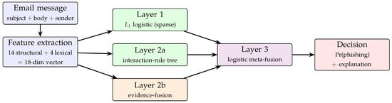
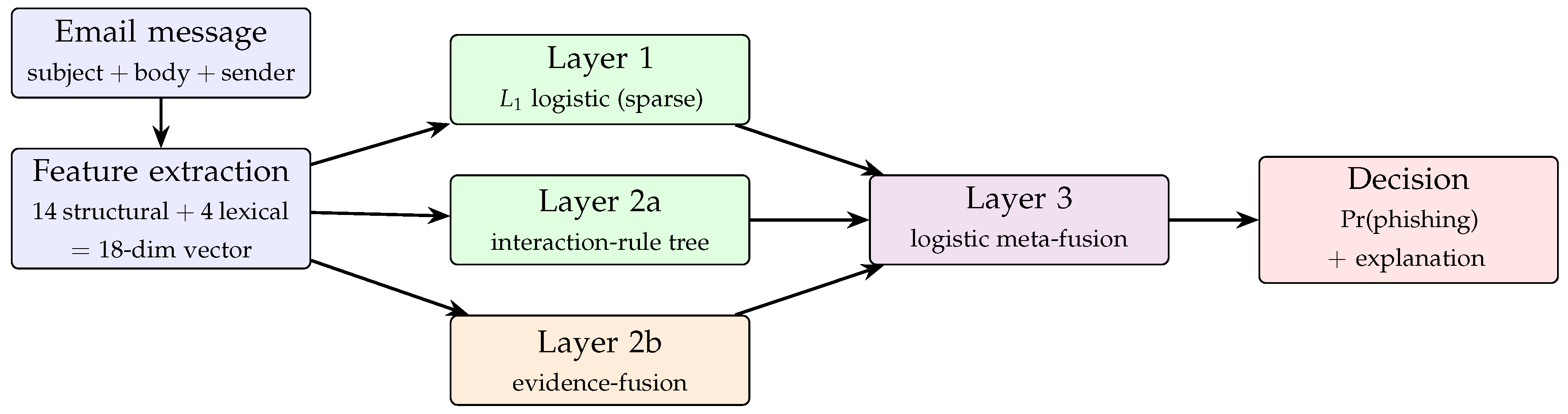
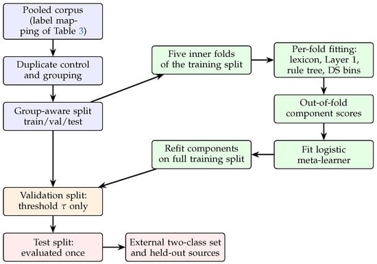
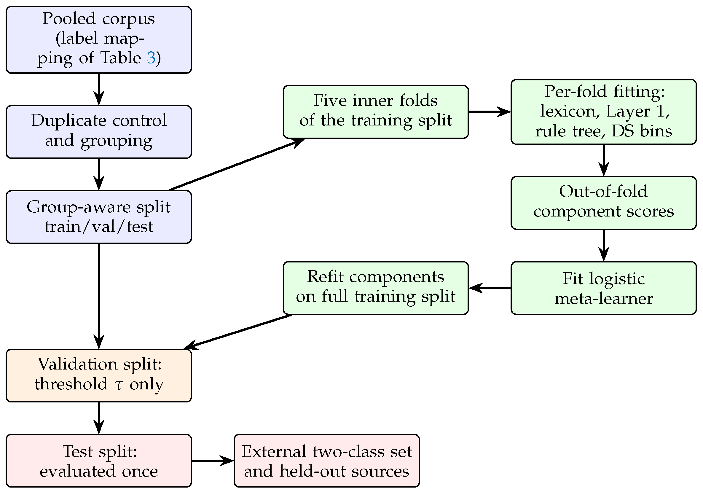
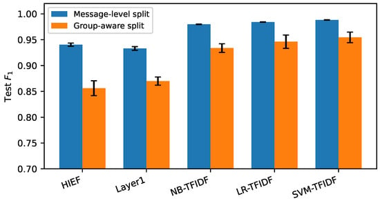
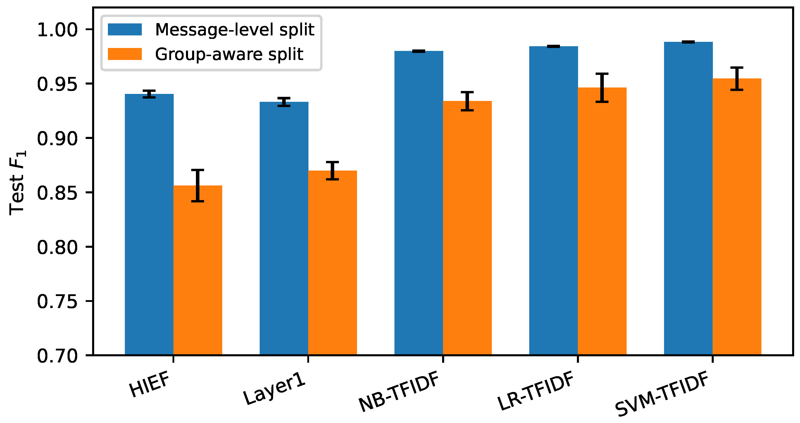
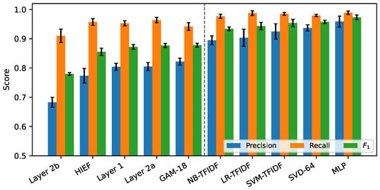
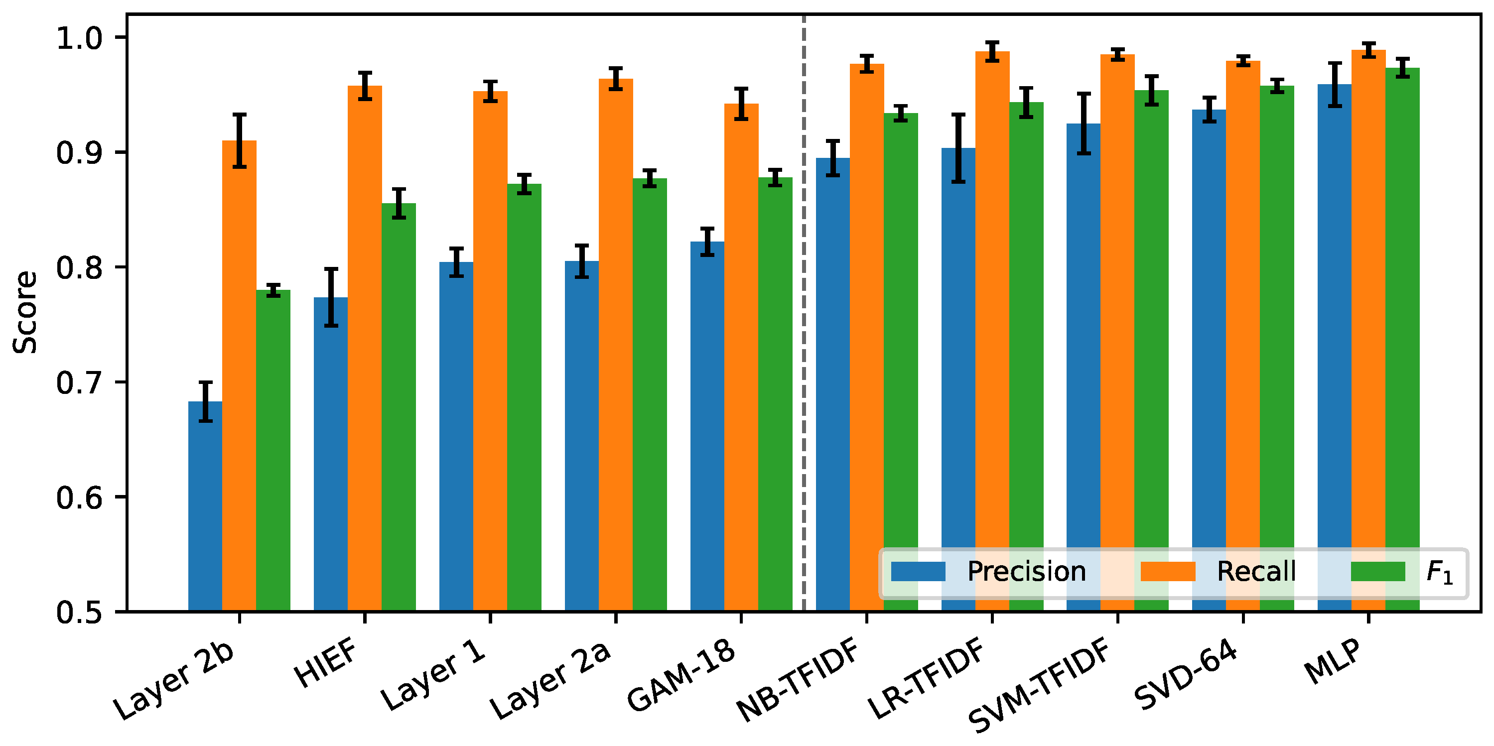
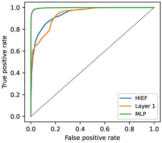
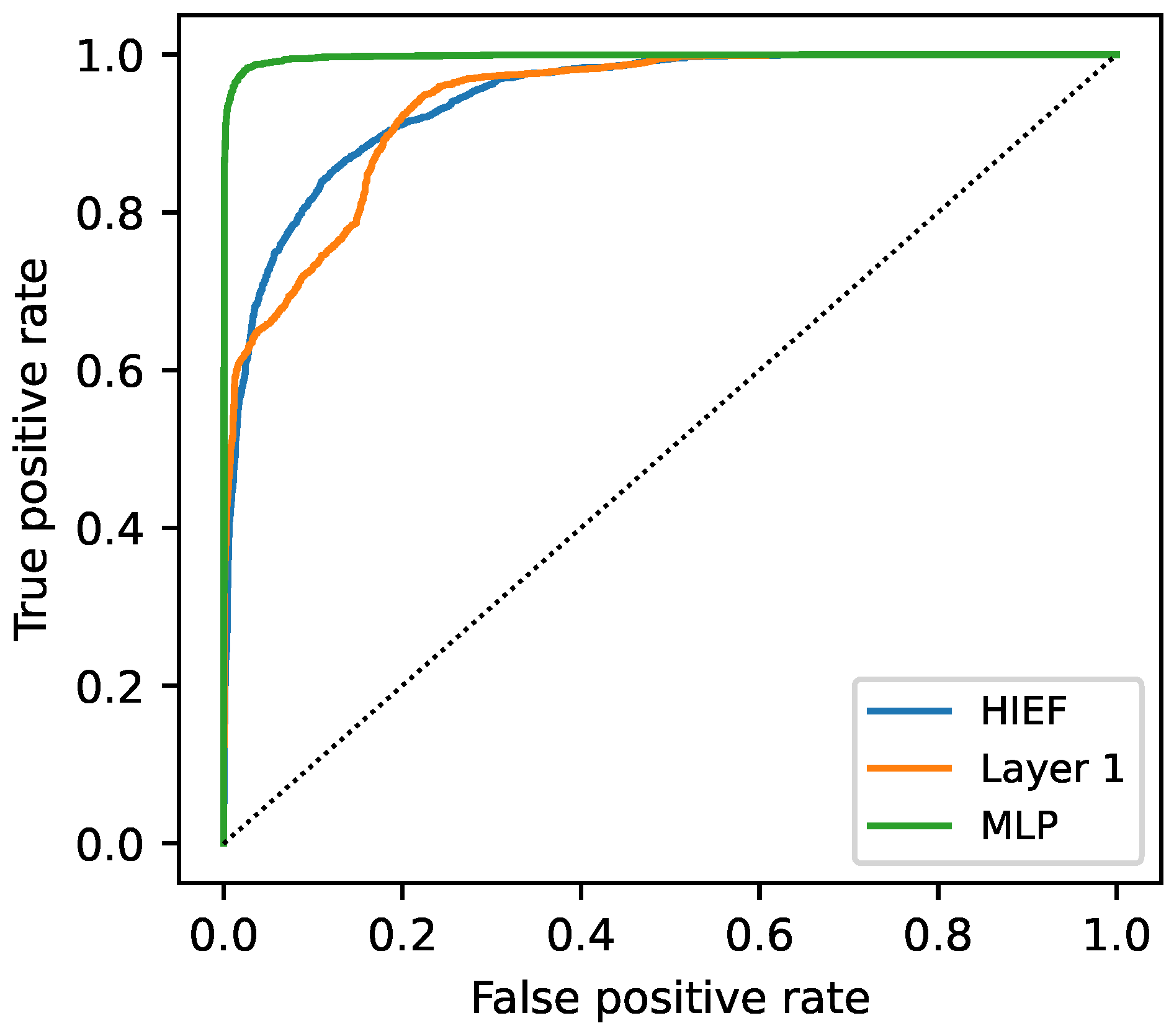
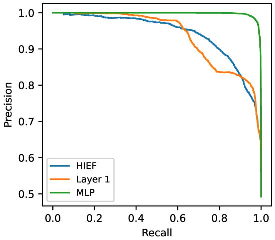
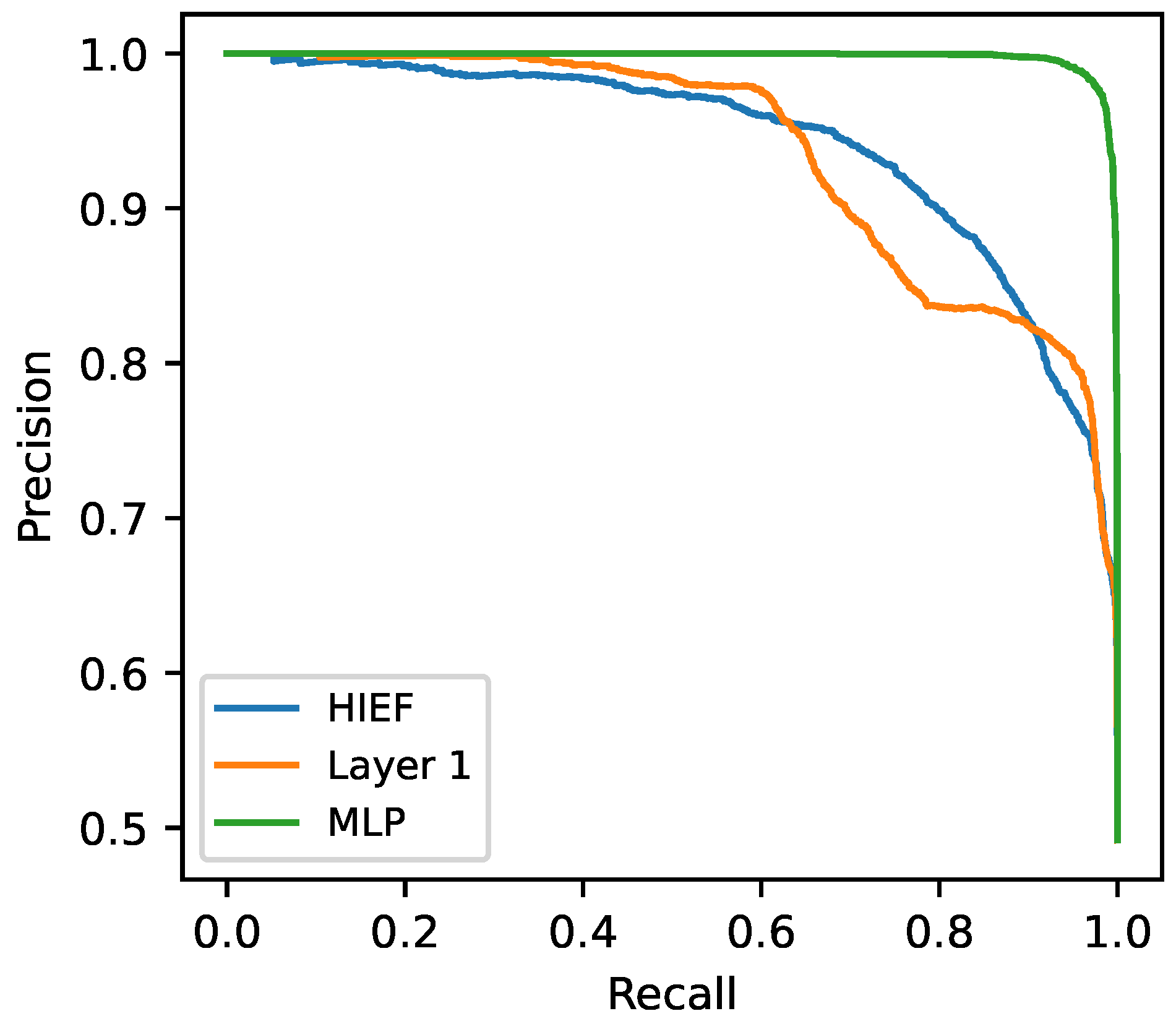
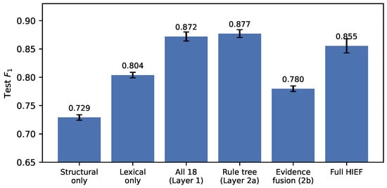
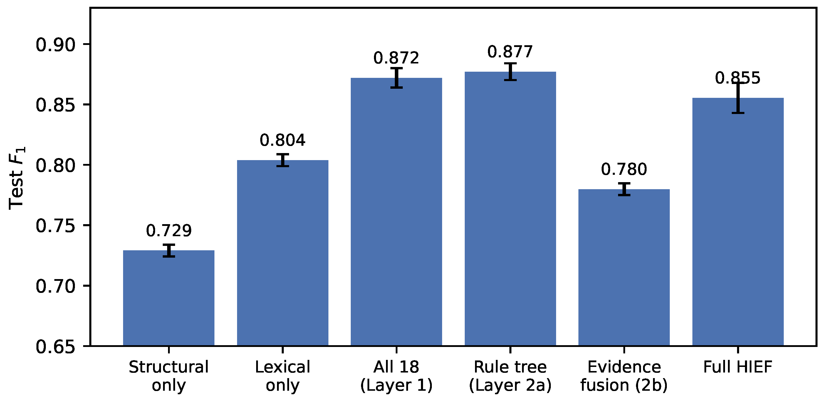
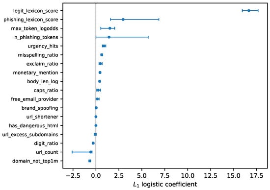
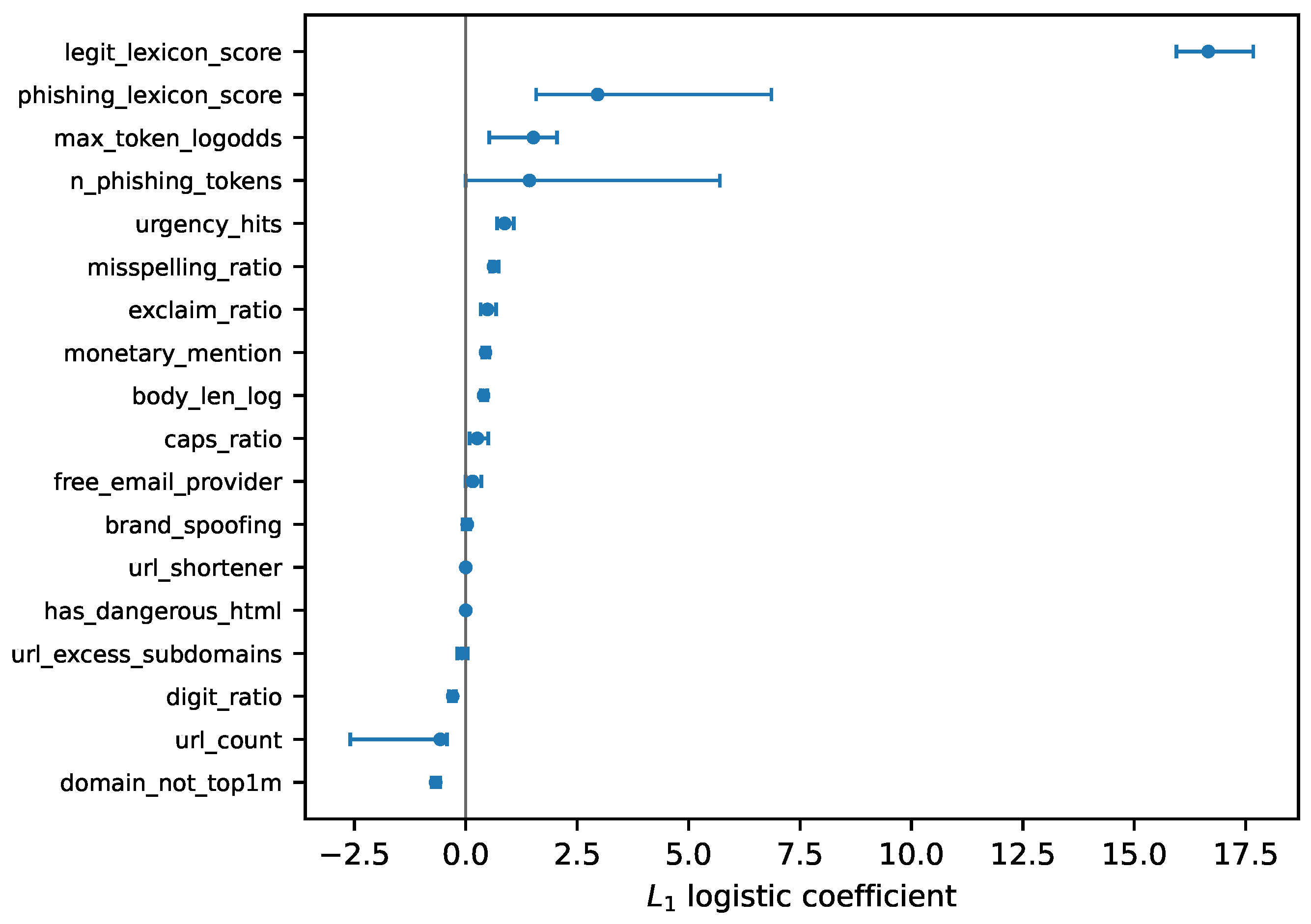
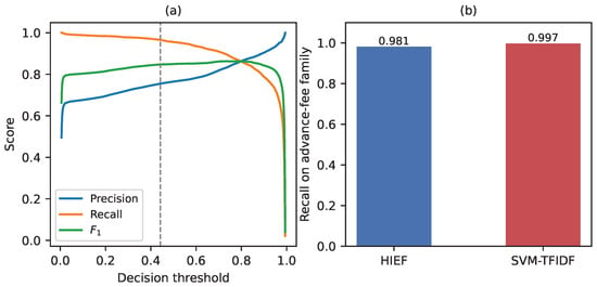
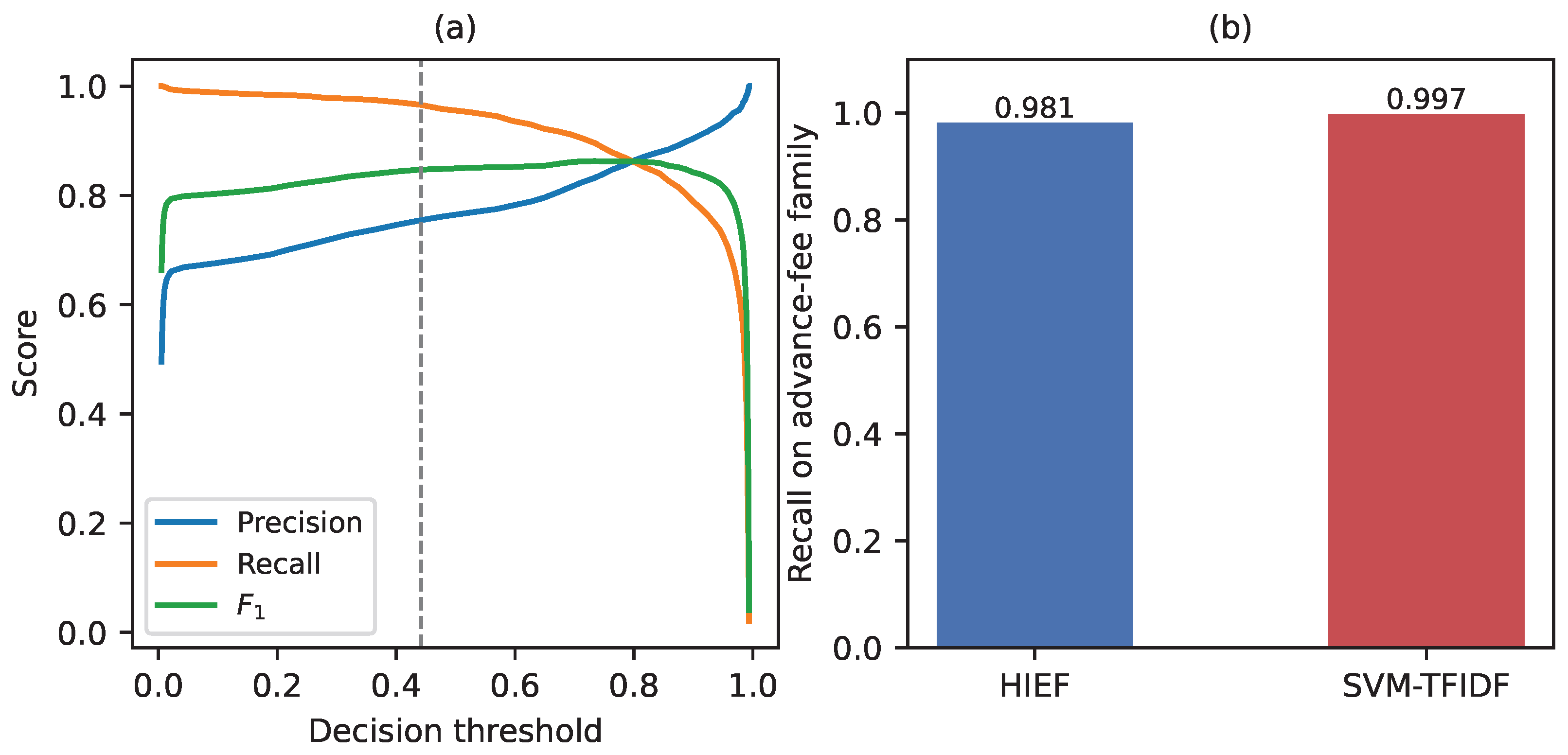
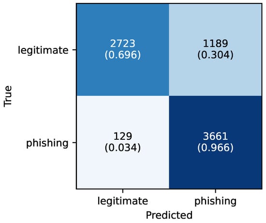
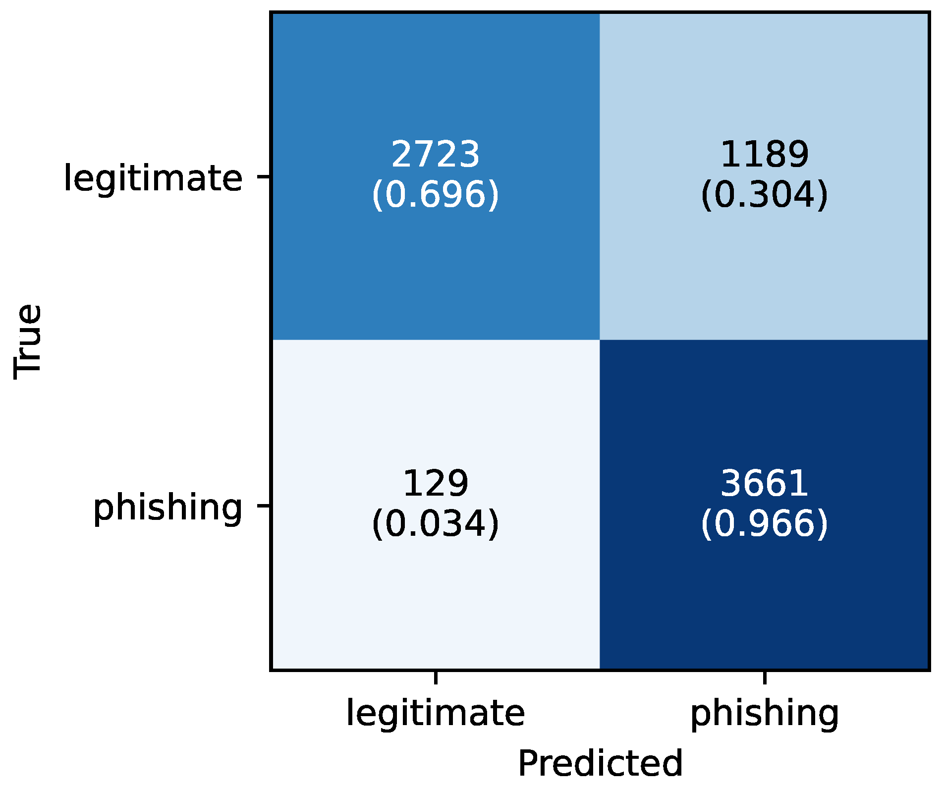
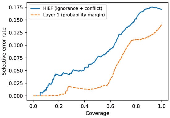
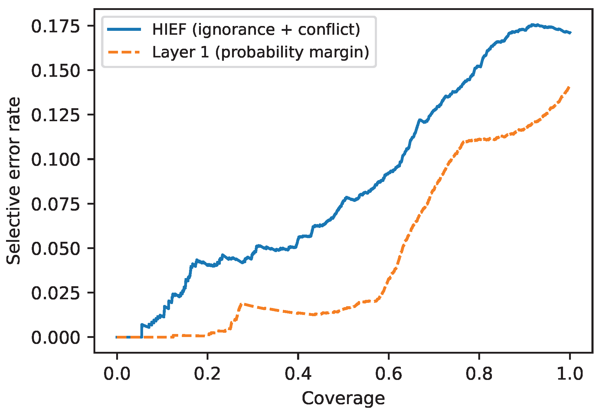

Disclaimer/Publisher’s Note: The statements, opinions and data contained in all publications are solely those of the individual author(s) and contributor(s) and not of MDPI and/or the editor(s). MDPI and/or the editor(s) disclaim responsibility for any injury to people or property resulting from any ideas, methods, instructions or products referred to in the content. |
© 2026 by the authors. Licensee MDPI, Basel, Switzerland. This article is an open access article distributed under the terms and conditions of the Creative Commons Attribution (CC BY) license.