Ultrasonic Lamb Wave Denoising Algorithm for Aluminum Plates Based on ICPO-VMD Combined Improvement of Wavelet Threshold

Abstract

In ultrasonic Lamb wave non-destructive testing of aluminum plates, Lamb wave signals are susceptible to industrial interference, which may obscure useful information. To address this issue, this paper developed a signal denoising method combining Improved Crested Porcupine Optimizer (ICPO) and Variational Mode Decomposition (VMD) with an improved wavelet threshold. The ICPO algorithm optimizes VMD parameters using fuzzy entropy as the fitness function. The decomposed modes are categorized into signal-dominant, mixed, and noise-dominant modes by the correlation coefficient method. The mixed modes are denoised using wavelet thresholding, and the final signal is reconstructed from the signal-dominant modes and the denoised mixed modes. Compared with VMD, direct wavelet thresholding, and ICPO-VMD combined with soft or hard thresholding, the proposed method outperforms the compared methods in both quantitative metrics and waveform preservation. These results confirm the effectiveness of the proposed method for aluminum plate Lamb wave denoising under the tested conditions.

1. Introduction

Ultrasonic testing technology has gained widespread application in the field of non-destructive testing due to its advantages of ease of operation, strong penetration capability, and high detection sensitivity [1]. Ultrasonic Lamb waves exhibit propagation characteristics such as extensive propagation range and low attenuation within aluminum plate structures [2]. These advantages make Lamb waves the preferred method for detecting defects in aluminum plates. However, in industrial practice, Lamb wave signals are often disrupted by multi-source noise [3], significantly compromising the accuracy and reliability of inspection results, making signal feature extraction critically important in Lamb wave non-destructive testing [4].

Ultrasonic Lamb wave signals typically exhibit nonlinear and non-stationary behavior during propagation [5] and also exhibit multimodal characteristics. These features make Lamb wave signals susceptible to noise interference, making noise reduction for these signals essential [6]. Currently, there are several commonly used methods in the field of signal denoising, such as the Fourier transform (FT) [7], wavelet transform (WT) [8], empirical mode decomposition (EMD) [9], and variational mode decomposition (VMD) [10]. Among these, FT serves to map temporal waveforms onto their corresponding spectral components, thereby precisely identifying the primary frequency components of the signal. However, the theory of FT is based on stationary signals; hence, it is incapable of reflecting the time-dependent behavior of non-stationary signals [11]. In contrast, the wavelet transform affords joint time–frequency localization. Its basis functions can be scaled and translated in both time and magnitude [12], enabling effective analysis of non-stationary signals. The wavelet thresholding method is the most common approach in wavelet transform-based denoising techniques. This method first decomposes the signal into wavelets; thresholding is subsequently performed on the wavelet coefficients to achieve denoising [13].

EMD adaptively splits complex signals into several intrinsic modal functions (IMFs) based on their inherent characteristics. Guo et al. [14] applied EMD to the detection and localization of leaks in water supply pipelines, effectively reducing the error in pinpointing leak locations. However, during decomposition, EMD is plagued by mode mixing and boundary effects [15]. To address this shortcoming, Konstantin and Zosso [16] proposed the VMD. This method effectively decomposes the signal into several band-limited IMFs through the formulation and optimization of a constrained variational framework. Due to its superior modal separation capability, noise resistance, and result stability, VMD has emerged as a predominant technique in signal processing. Zhou et al. [17] proposed using VMD to decompose vibration signals of rotating machinery. Experiments confirm that this method accurately captures signal features while removing noise. Wang et al. [18] employed VMD to suppress sea noise in ship axis velocity signals. In comparison, VMD outperforms discrete wavelet transform and EMD in signal processing capability.

However, two user-defined parameters, namely the mode number K and the penalty factor α, have a significant influence on the performance of VMD, and thus the outcomes often exhibit a strong degree of subjectivity [19]. To address this issue, numerous scholars have proposed various optimization algorithms. Hu et al. [20] employed the Gray Wolf Optimization (GWO) algorithm to optimize VMD parameters for wind turbine gearbox vibration signals. The optimized VMD offered better decomposition performance and maintained the main features of the signal. In 2024, Mohamed Abdel Basset et al. [21] proposed the CPO optimization algorithm, which achieves optimization by emulating the four defensive responses of the crown porcupine, demonstrating strong global search capabilities. However, when confronted with more complex signal processing tasks, traditional CPO may exhibit insufficient adaptability and slow convergence speed. Therefore, optimization strategies can be incorporated to enhance its ability to find optimal solutions [22] and further enhance the decomposition effect of VMD. In these optimization frameworks, choosing an appropriate fitness function is equally critical. Fuzzy entropy, as a nonlinear metric characterizing the complexity and regularity of time series [23], has been widely adopted as an effective fitness function in signal processing. Zhou et al. [24] employed fuzzy entropy as the fitness function to optimize VMD parameters, achieving improved decomposition and better denoising performance for sensor noise reduction in MEMS accelerometer signals.

Additionally, during the VMD decomposition process, noise components are likely to be assigned to IMF components, leading to the loss of signal detail [25], which will have a negative impact on subsequent analysis. As briefly introduced earlier, the wavelet thresholding method demonstrates strong noise suppression capabilities across different scales. Consequently, numerous studies in recent years have combined the two approaches to simultaneously enhance signals and suppress noise while separating different modal components of the signal.

Although the above hybrid optimization-based VMD-wavelet thresholding frameworks have achieved satisfactory results in various engineering fields, their direct application to ultrasonic Lamb wave signals still faces three critical limitations. First, optimization algorithms with poor search capability often fail to achieve thorough VMD decomposition, resulting in mode mixing and loss of effective information. Second, most existing frameworks treat all IMF components uniformly after VMD decomposition, typically applying wavelet thresholding to all IMFs or simply discarding low-energy components. However, Lamb wave signals contain multiple physical propagation modes, and low-amplitude components may carry critical defect information rather than being purely noise. Third, both traditional soft thresholding methods [26] and hard thresholding methods [27] have their own limitations. Hard thresholding methods may cause significant signal oscillation due to function discontinuity; soft thresholding methods may result in signal feature loss due to constant bias [28], which can distort the envelope shape of Lamb wave tone-burst signals and compromise subsequent feature extraction.

To address these limitations, this paper proposes an improved denoising framework with three specific methodological advances over existing hybrid approaches. First, an improved CPO strategy combining fuzzy entropy as the fitness function is adopted for VMD parameter optimization. Compared with conventional approaches, this strategy can decompose the signal more thoroughly. Second, a correlation-coefficient-based three-level classification scheme is developed to separate IMFs into signal modes, mixed modes, and noise modes. This ensures that IMFs with relatively low correlation coefficients but physically meaningful Lamb wave information are preserved rather than discarded, a critical requirement for multimodal signal processing. Third, an improved wavelet threshold function with adaptive adjustment is designed to overcome the discontinuity of hard thresholding and the constant bias of soft thresholding, thereby preserving the tone-burst envelope while effectively suppressing noise. These advances collectively make the proposed method particularly suitable for Lamb wave signal denoising, where preserving both modal components and waveform morphology is essential for reliable defect characterization. In summary, the key novelties of this study include:

• An improved crested porcupine optimizer (ICPO) algorithm is developed with dynamic parameter adjustment and random perturbation as algorithmic innovations, while parallel computing is employed as an implementation strategy to accelerate optimization.
• A correlation-based three-level IMF classification scheme is proposed to separate IMFs into signal-dominant, mixed, and noise-dominant modes.
• An improved wavelet threshold function with adaptive adjustment is designed to overcome the discontinuity and constant bias of conventional thresholding.

2. Basic Principles

2.1. Variational Mode Decomposition

VMD formulates a constrained variational framework, where the input signal is decomposed into multiple IMFs through an iterative variational optimization procedure, each of which is confined to a finite bandwidth. Unlike EMD decomposition, each mode in VMD decomposition is represented as a function with both amplitude and frequency modulation, as given by Equation (1):

$$u_k\left(t\right) ={ A}_k\left(t\right)\cos \left({\phi }_k\left(t\right)\right)$$

(1)

where${ u}_k\left(t\right)$represents the mode component,${ A}_k\left(t\right)$denotes the envelope amplitude of the IMF, and${ \phi }_k\left(t\right)$ signifies the instantaneous phase of the IMF. The method for establishing and solving the variational problem proceeds as follows:

First, each modal component is transformed via the Hilbert transform to derive its analytical signal. Subsequently, the corresponding unilateral spectral function$\eta \left(t\right)$is calculated to describe the signal’s components and amplitude in the frequency domain, as expressed mathematically in Equation (2):

$$\begin{array}{c}\eta \left(t\right)=\left(\delta \left(t\right)+{\displaystyle \frac{j}{\pi t}}\right)u_k\left(t\right)\end{array}$$

(2)

where $\delta \left(t\right)$is the impact function.

Then, a frequency shift of each mode’s unilateral spectrum is performed by multiplying$\eta \left(t\right)$by the complex exponential of the derived center frequency, shifting every IMF’s center frequency to the baseband. This process is given by Equation (3):

$${\hat{u}}_k\left(t\right)=\left[\left(\delta \left(t\right)+{\displaystyle \frac{j}{\pi t}}\right)u_k\left(t\right)\right]e^{-j{\omega }_{k}t}$$

(3)

where${\omega }_k$ denotes the k-th center frequency.

For each mode, the bandwidth is characterized using the squared L2 norm of the gradient, establishing a constrained variational optimization problem as shown in Equation (4):

$$\begin{array}{r}\{\begin{array}{l}\underset{\left\{u_k\right\},\left\{{\omega }_k\right\}}{\min }\left\{{{\displaystyle \sum _{k=1}^K}\Vert {\partial }_t\left[\left(\delta \left(t\right)+{\displaystyle \frac{j}{\pi t}}\right)*u_k\left(t\right)\right]{\mathrm{e}}^{-j{\omega }_{k}t}\Vert }_2^2\right\}\\ \mathrm{s}.\mathrm{t}.{\displaystyle \sum _{k=1}^K}{u}_k=f\end{array}\end{array}$$

(4)

where $K$ denotes the number of IMFs, $f$ represents the input signal, and $*$ denotes convolutional symbol.

The constrained variational formulation is converted into an augmented Lagrangian problem by introducing the penalty factor α and a Lagrange multiplier$\lambda \left(t\right)$, thereby reformulating it as an unconstrained problem for solution. The augmented Lagrangian is expressed as Equation (5):

$$\begin{array}{c}L\left(u_k,{\omega }_k,\lambda \left(t\right)\right)=\alpha {{\displaystyle \sum _{k=1}^K}\Vert {\partial }_t\left[\left(\delta \left(t\right)+{\displaystyle \frac{j}{\pi t}}\right)*u_k\left(t\right)\right]{\mathrm{e}}^{-j{\omega }_{k}t}\Vert }_2^2+{\Vert f\left(t\right)-{\displaystyle \sum _{k=1}^K}{u}_k\left(t\right)\Vert }_2^2\\ +⟨\lambda \left(t\right),f\left(t\right)-{\displaystyle \sum _{k=1}^K}{u}_k\left(t\right)⟩\end{array}$$

(5)

The mode numbers, center frequencies, and Lagrange multipliers are updated iteratively within the framework of the alternating direction method of multipliers. The process terminates upon meeting the stopping criteria, as expressed in Equations (6)–(9):

$${\hat{u}}_k^{n+1}\left(\omega \right)={\displaystyle \frac{\hat{f}\left(\omega \right)-{\sum }_{i\ne k}{\hat{u}}_i\left(\omega \right)+\hat{\lambda }\left(\omega \right)/2}{1+2\alpha {\left(\omega -{\omega }_k\right)}^2}}$$

(6)

$${\omega }_k^{n+1}={\displaystyle \frac{{\int }_0^{\infty }\omega {\left|{\hat{u}}_k(\omega )\right|}^2 \mathrm{d}\omega }{{\int }_0^{\infty }{\left|{\hat{u}}_k\left(\omega \right)\right|}^2 \mathrm{d}\omega }}$$

(7)

$${\hat{\lambda }}^{n+1}\left(\omega \right)={\hat{\lambda }}^n\left(\omega \right)+\tau \left(\hat{f}\left(\omega \right)-\sum _k{\hat{u}}_k^{n+1}\left(\omega \right)\right)$$

(8)

$$\sum _k{\displaystyle \frac{{\Vert {\hat{u}}_k^{n+1}-{\hat{u}}_k^n\Vert }_2^2}{{\Vert {\hat{u}}_k^n\Vert }_2^2}}<\epsilon$$

(9)

where$\hat{f}\left(\omega \right)$, ${\hat{u}}_k\left(\omega \right)$, and $\hat{\lambda }\left(\omega \right)$ respectively denote the Fourier transforms of $f\left(t\right)$, $u_k\left(t\right),$ and $\lambda \left(t\right)$,$\tau$is the stride parameter, and$\epsilon$is the termination threshold.

2.2. Crested Porcupine Optimizer Algorithm

The CPO algorithm is inspired by four cardinal defense mechanisms exhibited by the crested porcupine—namely, visual deterrence, auditory alarm, olfactory signaling, and direct physical retaliation [21]—thereby effectively balancing the exploration and exploitation phases within the search space. The specific algorithm can be explained in the following three stages:

• Initialization phase

At the initial stage of the CPO algorithm, a population of crown porcupines is randomly generated within the search boundaries. Each individual represents a candidate solution, and each candidate solution$X_i$is generated randomly within the search boundaries, as illustrated in Equation (10).

$$\overrightarrow{X_i}=\overrightarrow{L}+\overrightarrow{r}\left(\overrightarrow{U}-\overrightarrow{L}\right),i=1,2,\dots N$$

(10)

where$N$indicates the population size,$X_i$denotes the i-th candidate solution in the solution boundaries,$\overrightarrow{L}$and $\overrightarrow{U }$ are lower and upper search bounds, and $\overrightarrow{r}$ indicates a stochastic vector, with each component constrained to the interval [0, 1].

2.

Exploration phase

The visual deterrence strategy is designed for global exploration. Equation (11) represents the crown porcupine’s position update formula:

$$\overrightarrow{X_i^{t+1}}=\overrightarrow{X_i^t}+{\tau }_1\times \left|2\times {\tau }_2\times \overrightarrow{X_{\mathit{CP}}^t}-\overrightarrow{y_i^t}\right|$$

(11)

$\mathrm{w}\mathrm{h}\mathrm{e}\mathrm{r}\mathrm{e} \overrightarrow{X_i^{t+1}}$indicates the current solution,${ \tau }_1$is a number that follows a normal distribution,${\tau }_2$is generated from a uniform distribution with a range of (0, 1),$\overrightarrow{X_{\mathit{CP}}^t}$denotes the optimal solution recorded by the algorithm during the t-th function evaluation, and$\overrightarrow{y_i^t}$denotes the location of the predator in the t-th iteration.

The auditory alarming strategy is also designed for exploration to enhance population diversity, with the position evolution equation given by Equation (12):

$$\overrightarrow{x_i^{t+1}}=\left(1-\overrightarrow{U_1}\right)\times \overrightarrow{x_i^t}+\overrightarrow{U_1}\times \left(\overrightarrow{y_i^t}+{\tau }_3\times \left(\overrightarrow{x_{r1}^t}-\overrightarrow{x_{r2}^t}\right)\right)$$

(12)

$\mathrm{where} \overrightarrow{U_1}$is a binary vector containing only 0s and 1s,${\tau }_3$ represents a random variable obeying a normal distribution, and r1 and r2 represent two integers randomly drawn from the interval [1, N].

3.

Development phase

The olfactory signaling strategy is designed for local exploitation. The odor defense position is updated according to Equation (13):

$$\overrightarrow{x_i^{t+1}}=\left(1-\overrightarrow{U_1}\right)\times \overrightarrow{x_i^t}+\overrightarrow{U_1}\times \left(\overrightarrow{x_{r1}^t}+S_i^t\times \left(\overrightarrow{x_{r2}^t}-\overrightarrow{x_{r3}^t}\right)-{\tau }_3\times \overrightarrow{\delta }\times {\gamma }_t\times S_i^t\right)$$

(13)

here,$\overrightarrow{x_i^t}$denotes the location vector associated with the i-th search agent in iteration t, r3 represents a random number within the range [1, N],$\overrightarrow{\delta }$is a vector that regulates the search tendency,${\gamma }_t$ represents the defense coefficient,$S_i^t$indicates the odor diffusion coefficient, and ϵ is a minimum value preventing division by zero. The specific expressions are shown in Equations (14)–(16):

$$\overrightarrow{\delta }=\{\begin{array}{c}+1,\mathrm{i}\mathrm{f} \mathrm{rand}\le 0.5\\ -1,\mathrm{Else}\end{array}$$

(14)

where rand is a uniformly distributed random number in [0, 1].

$${\gamma }_t=2\times \mathrm{rand}\times {\left(1-{\displaystyle \frac{t}{t_{\max }}}\right)}^{{\displaystyle \frac{t}{t_{\max }}}}$$

(15)

$$S_i^t=\exp \left({\displaystyle \frac{\mathrm{f}\left(x_i^t\right)}{{\displaystyle {\sum }_{k=1}^N}f\left(x_k^t\right)+ϵ}}\right)$$

(16)

where t is the current iteration number,$t_{\max }$ is the maximum number of iterations, and $f\left(x_i^t\right)$ denotes the fitness value of the $i$-th individual at iteration t.

The physical retaliation strategy is designed for exploitation to accelerate convergence. Equation (17) shows how the position is updated during the fourth stage direct physical retaliation:

$$\overrightarrow{x_i^{t+1}}=\overrightarrow{x_{\mathit{CP}}^t}+\left(\alpha (1-{\tau }_4)+{\tau }_4\right)\times \left(\delta \times \overrightarrow{x_{\mathit{CP}}^t}-\overrightarrow{x_i^t}\right)-{\tau }_5\times \delta \times {\gamma }_t\times \overrightarrow{F_i^t}$$

(17)

$$\overrightarrow{F_i^t}=\overrightarrow{{\tau }_6}\times m_i\times \left(v_i^{t+1}-v_i^t\right)$$

(18)

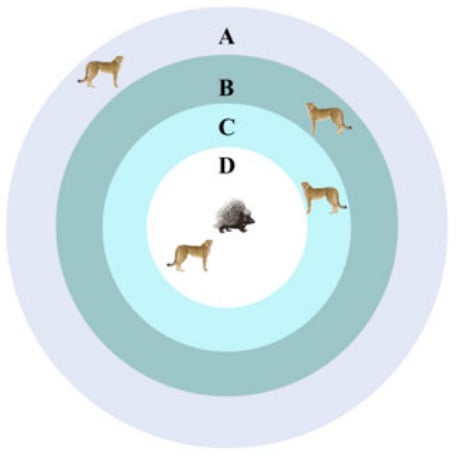
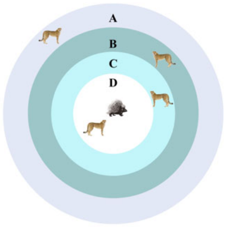
where $\overrightarrow{x_{\mathit{CP}}^t}$denotes the optimal solution at iteration t, α is the convergence rate factor in [0, 1] (with a default value of 0.2 in this study), ${\tau }_4$ and ${\tau }_5$ are random numbers between 0 and 1, and$\overrightarrow{F_i^t}$represents the average force exerted by the i-th predator, as shown in Equation (18).$\overrightarrow{{\tau }_6}$denotes a random vector with entries uniformly distributed between 0 and 1. The mass of the i-th individual is denoted by$m_i$, $v_i^{t+1}$denotes the final velocity of the i-th individual in the subsequent iteration, while$v_i^t$ denotes the terminal velocity in the current iteration. The four specific defense mechanisms are illustrated in Figure 1.

Figure 1. CPO defense mechanism: Four defense mechanisms of the crested porcupine optimizer (CPO) algorithm: visual deterrence (A), auditory alarming (B), olfactory signaling (C), and physical retaliation (D) (adapted from [21] with modifications).

2.3. Fuzzy Entropy

As a nonlinear metric, fuzzy entropy characterizes the complexity and regularity inherent in time series data. It can be used as an adaptability function in optimization algorithms, defined as follows:

• Let the N-point sampling sequence be$\left\{u\left(i\right):1\le i\le N\right\}$, generating an m-dimensional vector in sequence according to Equation (19). Equation (20) represents the mean of the vector within the brackets.

  $$X_i^m=\left\{u\left(i\right),u\left(i+1\right),\cdots ,u\left(i+m-1\right)\right\}-u_0\left(i\right) \left(i=1,\cdots ,N-m\right)$$

  (19)

  $$u_0\left(i\right)={\displaystyle \frac{1}{m}}{\displaystyle \sum _{j=0}^{m-1}}u\left(i+j\right)$$

  (20)
• Define the distance$\mathrm{d}\left[X_i^m,X_j^m\right]$ between$X_i^m$ and$X_j^m$ as the maximum value of their difference, as shown in Equation (21):

  $$\mathrm{d}\left[X_i^m,X_j^m\right]=\max \left\{\left|\left(u\left(i+k\right)-u_0\left(i\right)\right)-\left(u\left(j+k\right)-u_0\left(j\right)\right)\right|\right\}$$

  (21)
• The fuzzy membership function is defined as$D_{\mathit{ij}}^m=\mu \left(d_{\mathit{ij}},r,n\right)=e^{\left(-{\left({\displaystyle \frac{d_{\mathit{ij}}}{r}}\right)}^n\right)}$, where n controls the gradient of the exponential membership boundary and r governs its width.
• Define the average similarity function as shown in Equation (22):

  $${\phi }_m\left(r\right)={\displaystyle \frac{1}{N-m}}{\displaystyle \sum _{i=1}^{N-m}}\left({\displaystyle \frac{1}{N-m-1}}{\displaystyle \sum _{j=1,j\ne i}^{N-m}}{D}_{\mathit{ij}}^m\right)$$

  (22)
• Fuzzy entropy is expressed as shown in Equation (23):

  $$\mathrm{FuzzyEn}\left(m,n,r\right)=\underset{N\to \infty }{\lim }\left[\ln {\phi }_m\left(r\right)-\ln {\phi }_{m+1}\left(r\right)\right]$$

  (23)

2.4. Correlation Coefficient

The correlation coefficient assesses how closely each component correlates with the initial data. The lower the correlation coefficient, the fewer characteristics of the overall data contained within that component; higher correlation coefficients indicate components that better preserve the original signal features. The correlation coefficient is computed as:

• Calculate covariance

$$\mathrm{cov}\left(x,I_k\right)={\displaystyle \frac{1}{N-1}}{\displaystyle \sum _{i=1}^N}\left(x_i-\stackrel{\mathrm{-}}{x}\right)\left(I_{\mathit{ki}}-\overline{I_k}\right)$$

(24)

here,$\overline{x}$ and $\overline{I_k}$represent the arithmetic mean of the original signal and the $k$-th IMF function, respectively.

2.

Calculate the standard deviation

$${\sigma }_x=\sqrt{{\displaystyle \frac{1}{N-1}}{\displaystyle \sum _{i=1}^N}{\left(x_i-\stackrel{\mathrm{-}}{x}\right)}^2},{\sigma }_{I_k}=\sqrt{{\displaystyle \frac{1}{N-1}}{\displaystyle \sum _{i=1}^N}{\left(I_{\mathit{ki}}-\overline{I_k}\right)}^2}$$

(25)

where${\sigma }_x$and${\sigma }_{I_k}$denote the standard deviations of the original signal and the corresponding IMF components, respectively.

3.

Calculate the correlation coefficient

$${\rho }_k={\displaystyle \frac{\mathrm{cov}\left(x,I_k\right)}{{\sigma }_x·{\sigma }_{I_k}}}$$

(26)

2.5. Wavelet Threshold

Wavelet-thresholding exploits the multi-resolution property of the wavelet transform to separate a noisy signal into multi-scale components. An appropriate threshold is then set based on the differences in coefficient magnitudes. Processing wavelet coefficients using thresholding functions preserves the primary signal components and reconstructs them to achieve noise reduction. The specific workflow is illustrated in Figure 2:

Figure 2. Wavelet threshold denoising workflow.

• Wavelet decomposition

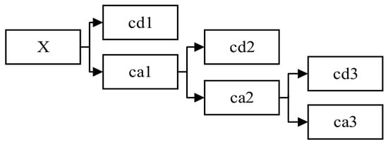
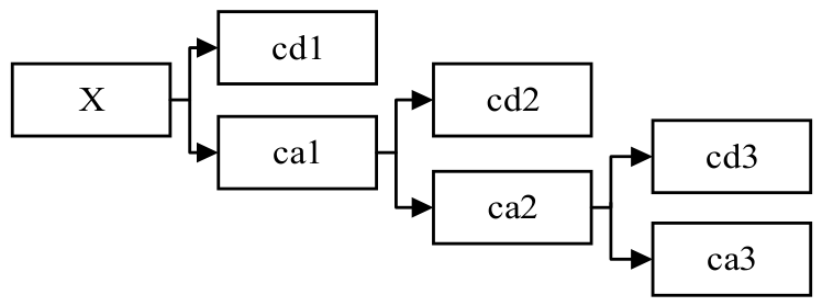
Wavelet decomposition uses high-pass and low-pass filters to progressively separate a noisy signal into approximation coefficients representing the trend and detail coefficients representing the fine features. Through multi-level decomposition, approximation coefficients are further decomposed into new approximation coefficients and detail coefficients, thereby better distinguishing the overall trend and local details of the signal. The specific process is illustrated in Figure 3:

Figure 3. Wavelet decomposition process, where X is the noisy signal, cd is the detail coefficient, and ca is the approximation coefficient.

2.

Threshold processing

Threshold processing is central to wavelet threshold denoising. Selecting an appropriate threshold effectively removes noise while maximizing the preservation of signal features. This paper employed a fixed threshold for denoising, as expressed in Equation (27):

$$\lambda =\sigma \sqrt{2\ln \left(N\right)}$$

(27)

where$\sigma ={\displaystyle \frac{\mathrm{median}\left(\left|{\omega }_j\right|\right)}{0.6745}}$,${\omega }_j$denotes the detail coefficient for each decomposition, 0.6745 represents the median of the absolute values in the standard normal distribution, and in the calculation, the absolute median estimator is converted to the standard deviation σ. N denotes the signal length.

After selecting the threshold, each approximation coefficient obtained from the wavelet decomposition should undergo threshold processing. Conventional thresholding techniques consist of hard and soft thresholding functions. Among these, the hard threshold function is given as shown in Equation (28):

$${\hat{\omega }}_j=\{\begin{array}{c}{\omega }_j, \left|{\omega }_j\right|>\lambda ,\\ 0, \left|{\omega }_j\right|\le \lambda .\end{array}$$

(28)

Equation (29) gives the soft threshold function:

$${\hat{\omega }}_j=\{\begin{array}{c}\mathrm{sgn}\left({\omega }_j\right)\left(\left|{\omega }_j\right|-\lambda \right), \left|{\omega }_j\right|>\lambda ,\\ 0, \left|{\omega }_j\right|\le \lambda .\end{array}$$

(29)

where sgn refers to the sign function, and λ corresponds to the threshold.

The hard threshold method effectively preserves the sharp features and abrupt changes in a signal, but it can cause signal oscillations; soft thresholding achieves smoother denoising results by shrinking the wavelet coefficients, but it may result in the loss of some signal details. Overall, both hard threshold and soft thresholding methods possess their own advantages and limitations, making it challenging to strike a balance between noise suppression and feature preservation. This presents an avenue for research into improving threshold functions.

3.

Wavelet reconstruction

The essence of wavelet reconstruction lies in the inverse transformation of wavelet decomposition. Signal reconstruction involves combining the approximation coefficients of the deepest layer and the thresholded detail coefficients of each decomposition level.

3. Denoising Algorithm Based on Improved Wavelet Threshold Combined with ICPO-VMD

3.1. ICPO Optimization Algorithm

While the CPO algorithm performs well in solving standard optimization problems, several issues remain in practical applications:

• Computational efficiency needs improvement: Traditional CPO algorithms rely on serial computation, resulting in lengthy processing times and often low efficiency for large-scale optimization problems.
• Fixed parameters are difficult to select: In traditional CPO optimization algorithms, the convergence rate α and the proportion of the defense mechanism$T_f$are typically fixed. However, the initial search phase requires larger α and$T_f$values to enable rapid global exploration, while the late search phase necessitates smaller α and$T_f$values to achieve stable convergence. Therefore, fixed parameters cannot adapt to changes in the search space across different optimization stages, thereby affecting the algorithm’s stability and convergence speed.
• Prone to local optima: Traditional CPO algorithms employ multiple defense mechanisms to avoid local optima, with each individual position update driven by both the global optimum and interactions among individuals. However, in certain complex scenarios, when the algorithm approaches a local optimum, individual update steps may become too small or directionally constrained. This can cause the overall process to become trapped in a local optimum, preventing it from continuing to search for a better solution.

To overcome the issues above-mentioned, this paper presents three strategies to improve the optimization efficiency of the CPO algorithm, thereby providing more suitable parameters for subsequent VMD calculations.

• Utilizing parallel computing: In the improved CPO algorithm, the serial for-loop used for population fitness evaluation and iterative updates in the original algorithm has been rewritten as a parallel parfor structure. This enables the MATLAB Parallel Computing Toolbox to launch multiple worker processes and distribute different computational tasks evenly among these processes for simultaneous execution, thereby reducing the algorithm’s computation time.
• Dynamic adjustment of parameters: An α value capable of dynamic adjustment has been introduced into the improved CPO algorithm. This value decreases over time, with its mathematical expression shown in Equation (30):

  $${\alpha }_t={\alpha }_{\max }-\left({\alpha }_{\max }-{\alpha }_{\min }\right)·{\displaystyle \frac{t}{T_{\max }}}$$

  (30)

  $\mathrm{where} {\alpha }_{\max }$ and ${\alpha }_{\min }$ represent the maximum and minimum convergence rates, respectively, set to 0.9 and 0.2 in this experiment. $T_{\max }$ denotes the maximum iteration count.
  The algorithm also incorporates a dynamically adjustable defense mechanism ratio $T_f$, whose mathematical expression is shown in Equation (31):

  $$T_f\left(t\right)={T_f}_{\max }-\left({T_f}_{\max }-{T_f}_{\min }\right)·{\displaystyle \frac{t}{T_{\max }}}$$

  (31)
  $\mathrm{where} {T_f}_{\max }$ and ${T_f}_{\min }$ represent the maximum and minimum values of the defense mechanism ratio, respectively, which were set to 0.8 and 0.5 in this experiment.
• Introduction of random perturbations: A slight random perturbation is introduced into the improved CPO optimization algorithm. In this experiment, a random vector was added to the position of each individual with a 5% probability, enabling it to escape local optima and enhance search diversity. Equation (32) provides the specific formula:

  $$\overrightarrow{X_i^{t+1}}=\overrightarrow{X_i^t}+\sigma ·ϵ$$

  (32)

  where σ represents the perturbation amplitude of $0.01\times \left(\mathit{ub}-\mathit{lb}\right)$, and ϵ denotes a two-dimensional normal random vector with mean 0 and variance 1.

To quantify this benefit, the serial and parallel implementations were compared under identical conditions on an Intel Core i9-14900HX CPU (24 cores, 32 logical processors) with 32 GB RAM, running MATLAB R2024a with 8 parallel workers. The parallel implementation significantly reduces computation time without affecting the optimization results.

The above parameters were determined through preliminary experiments. A sensitivity analysis confirmed that the algorithm’s performance remained stable under reasonable parameter variations.

By incorporating the above three improvement strategies, the ICPO optimization algorithm achieves rapid convergence when tackling complex optimization problems, enabling it to promptly escape local optima and enhance the algorithm’s adaptability.

3.2. Parameter Optimization of ICPO-VMD

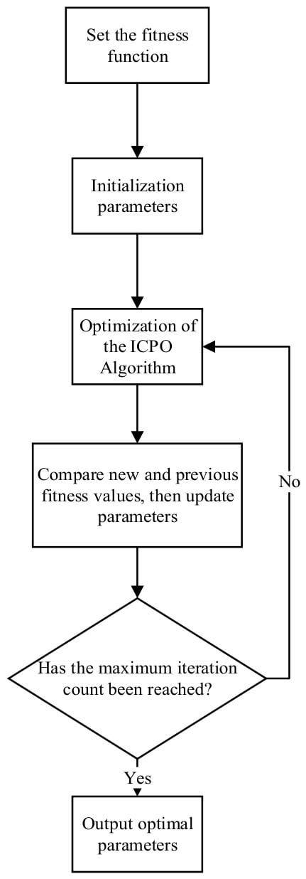
Although VMD decomposition can effectively achieve signal denoising, its performance depends strongly on the parameters K and α, where K determines the number of IMF functions obtained from the VMD decomposition. If K is set too large, the signal becomes over-decomposed, whereas a too-small K causes mode mixing. The penalty factor influences the mode bandwidth and center frequency. A higher value of α imposes a stronger bandwidth constraint, resulting in narrower modes, a smoother mode, and reduced ability to capture high-frequency noise; the smaller the α value, the wider the modal bandwidth, allowing the capture of more signal details. However, this also preserves noise, potentially resulting in less distinct modal separation. The ICPO was adopted to search the VMD decomposition parameters, with fuzzy entropy as the fitness function. The specific optimization steps of ICPO-VMD are illustrated in Figure 4.

Figure 4. ICPO-VMD optimization process.

• Set the fitness function

To enhance the decomposition results, the fitness function is constructed as the total fuzzy entropy of the IMF components derived from each VMD decomposition. The optimization objective is to minimize this fitness value, thereby identifying the optimal combination of parameters K and α.

2.

Initialization parameters

Initialize the parameters for the VMD and ICPO algorithms: population size = 20, maximum iterations = 30, search range for α = [100, 3000], and search range for K = [2, 15]. The population size and maximum iteration count are set based on preliminary experiments: a population of 20 provides sufficient search diversity while maintaining computational efficiency, and the ICPO algorithm typically converges within 30 iterations. The search range for K was set to [2, 15], covering the reasonable number of modes for Lamb wave signals, and α was searched within [100, 3000], covering the typical range reported in VMD-based signal processing literature. The same ranges were applied to all simulated and measured signals to ensure fair comparison.

3.

Parameter update

Each iteration of the ICPO optimization algorithm generates a new generation of candidate parameters $\left(K_i,{\alpha }_i\right)$, calculates their fitness values, and compares them with the fitness values of the corresponding individuals from the previous generation. If the new individual yields a lower fitness value, it replaces the original parameter set.

4.

Iteration termination

When the loop reaches the preset maximum iteration count, the iteration stops and outputs the final global optimal solution $\left(K^{*},{\alpha }^{*}\right)$ as the optimal parameters for the VMD decomposition.

3.3. Improved Wavelet Threshold Function

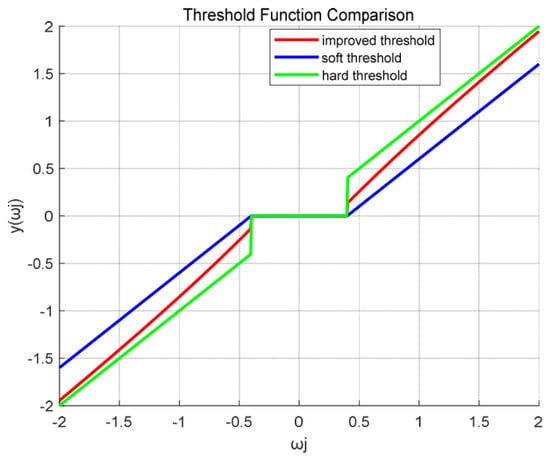
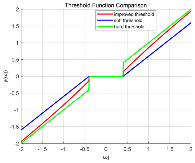
Although traditional wavelet thresholding algorithms are widely applied, their soft and hard thresholding functions each have limitations. Hard threshold functions are discontinuous at the threshold point, and reconstruction is prone to oscillation; although soft threshold functions are continuous, a constant bias always exists between the estimated and actual values, making them prone to errors. To address the limitations of the two thresholding methods, an improved threshold function is introduced. By introducing an adaptive factor, the threshold is dynamically tuned according to the amplitude variation of the signal. The threshold is designed according to the signal’s own amplitude characteristics, where the median amplitude represents the central tendency of the signal’s energy distribution and is more robust against extreme values. The threshold function is defined in Equation (33):

$${\hat{\omega }}_j=\{\begin{array}{c}\mathrm{sgn}\left({\omega }_j\right)·\left(\left|{\omega }_j\right|-\lambda ·{\mathrm{e}}^{-{\displaystyle \frac{\left|{\omega }_j\right|}{\mathrm{median}\left(\left|{\omega }_j\right|\right)+\epsilon }}}\right),\left|{\omega }_j\right|>\lambda \\ 0, \left|{\omega }_j\right|\le \lambda \end{array}$$

(33)

where the median of the amplitudes is denoted as $\mathrm{median}\left(\left|{\omega }_j\right|\right)$, and is adopted instead of the mean value because it is more robust to outliers and extreme values, which are commonly introduced by noise. ε represents a minimal value (set to 10⁻¹⁰ in this study) to prevent the denominator from becoming zero. A graphical comparison of the proposed threshold function with the traditional hard–soft pair is presented in Figure 5.

Figure 5. Comparison of threshold functions.

For the proposed threshold function, the asymptotic and bias properties are proven as follows:

• Progressivity

As${\omega }_j \mathrm{approaches} -\infty$, $\underset{{\omega }_j\to -\infty }{\lim }{\displaystyle \frac{{\hat{\omega }}_j}{{\omega }_j}}={\displaystyle \frac{-\left(\left|{\omega }_j\right|-\lambda ·{\mathrm{e}}^{-\frac{\left|{\omega }_j\right|}{\mathrm{median}\left(\left|{\omega }_j\right|\right)+\epsilon }}\right)}{{\omega }_j}}={\displaystyle \frac{{\omega }_j+\lambda ·{\mathrm{e}}^{-\frac{-{\omega }_j}{\mathrm{median}\left(-{\omega }_j\right)+\epsilon }}}{{\omega }_j}}=1+{\displaystyle \frac{\lambda ·{\mathrm{e}}^{\frac{{\omega }_j}{\mathrm{median}\left(-{\omega }_j\right)+\epsilon }}}{{\omega }_j}}=1$,

As${\omega }_j \mathrm{approaches} \infty$, $\underset{{\omega }_j\to \infty }{\lim }{\displaystyle \frac{{\hat{\omega }}_j}{{\omega }_j}}={\displaystyle \frac{\left|{\omega }_j\right|-\lambda ·{\mathrm{e}}^{-\frac{\left|{\omega }_j\right|}{\mathrm{median}\left(\left|{\omega }_j\right|\right)+\epsilon }}}{{\omega }_j}}={\displaystyle \frac{{\omega }_j-\lambda ·{\mathrm{e}}^{-\frac{{\omega }_j}{\mathrm{median}\left({\omega }_j\right)+\epsilon }}}{{\omega }_j}}=1-{\displaystyle \frac{\lambda ·{\mathrm{e}}^{-\frac{{\omega }_j}{\mathrm{median}\left({\omega }_j\right)+\epsilon }}}{{\omega }_j}}=1$,

Therefore,$\underset{{\omega }_j\to -\infty }{\lim }{\displaystyle \frac{{\hat{\omega }}_j}{{\omega }_j}}=\underset{{\omega }_j\to \infty }{\lim }{\displaystyle \frac{{\hat{\omega }}_j}{{\omega }_j}}=1$, so the proposed threshold function is characterized by the asymptote${\hat{\omega }}_j={\omega }_j$.

2.

Deviation

Since this threshold function is an odd function, when ${\omega }_j\to \pm \infty$:

$$\underset{{\omega }_j\to \infty }{\lim }\left({\hat{\omega }}_j-{\omega }_j\right)=\left({\omega }_j-\lambda ·{\mathrm{e}}^{-{\displaystyle \frac{{\omega }_j}{\mathrm{median}\left({\omega }_j\right)+\epsilon }}}\right)-{\omega }_j=-\lambda ·{\mathrm{e}}^{-{\displaystyle \frac{{\omega }_j}{\mathrm{median}\left({\omega }_j\right)+\epsilon }}}=0,$$

$$\underset{{\omega }_j\to -\infty }{\lim }\left({\hat{\omega }}_j-{\omega }_j\right)=\left(-1\right)\left(\left(-{\omega }_j\right)-\lambda ·{\mathrm{e}}^{-{\displaystyle \frac{-{\omega }_j}{\mathrm{median}\left(-{\omega }_j\right)+\epsilon }}}\right)-{\omega }_j=\lambda ·{\mathrm{e}}^{{\displaystyle \frac{{\omega }_j}{\mathrm{median}\left(-{\omega }_j\right)+\epsilon }}}=0.$$

The above equation demonstrates that the proposed threshold functions${\hat{\omega }}_j$ and${\omega }_j$ exhibit no constant bias, effectively mitigating the bias introduced by soft threshold functions in wavelet threshold denoising.

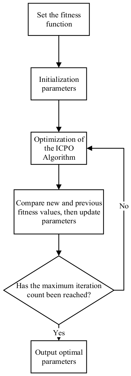
3.4. ICPO-VMD Hybrid-Based Improved Wavelet Threshold Denoising Algorithm

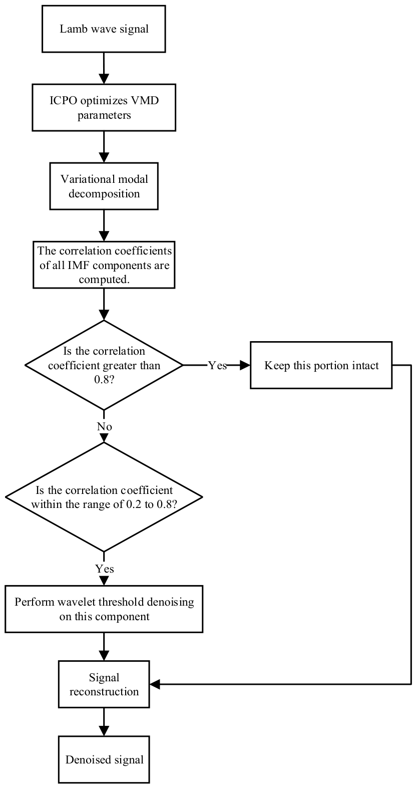
After obtaining the optimal parameters$\left(K^{*},{\alpha }^{*}\right)$ through ICPO algorithm optimization, the initial signal is decomposed by VMD into K* IMFs. Finally, the denoised signal is reconstructed by combining these IMF functions. However, to further enhance signal reconstruction quality, this paper proposes employing a correlation coefficient method to filter the multiple IMFs generated by ICPO-VMD decomposition.

After calculating the correlation coefficients of each IMF function, they are classified into three categories: signal mode, mixed mode, and noise mode. Among these, signal modes with higher correlation coefficients preserve the primary components of the signal and can be retained directly; mixed modes with moderate correlation coefficients simultaneously contain both minor signal components and noise, and therefore require wavelet threshold denoising for this portion of the signal; noise modes are typically regarded as noise-dominated components and are directly eliminated.

According to the experimental results reported in Xu et al. [29], when the correlation coefficient exceeds 0.8, the component exhibits a strong correlation with the original signal; when it falls below 0.2, the component is considered almost irrelevant to the original signal. Based on these criteria, the screening thresholds for the correlation coefficient in this study were set to 0.8 and 0.2. The specific process is as follows: IMFs with correlation coefficients above 0.8 are classified as signal-dominant modes and directly retained; IMFs with coefficients below 0.2 are classified as noise-dominant modes and discarded; and IMFs with coefficients in the intermediate range of 0.2 to 0.8 are classified as mixed modes requiring further wavelet threshold denoising. The overall procedure consists of the following steps:

• Parameter optimization: The optimal pair of VMD parameters—the mode number and penalty factor—is identified using the ICPO algorithm.
• Variational modal decomposition: Based on the optimal solution parameters derived from the ICPO optimization algorithm, the signal is separated into K IMF components.
• IMF selection: Calculate the correlation coefficients for K IMF components, then categorize them into three groups: those with coefficients above 0.8, those between 0.2 and 0.8, and those below 0.2. Components with coefficients above 0.8 are retained directly, while those below 0.2 are discarded outright.
• Wavelet threshold denoising: IMF components with correlation coefficients between 0.2 and 0.8 undergo wavelet threshold denoising before retention.
• Signal reconstruction: Reconstruct IMF components with correlation coefficients above 0.8 and IMF components after wavelet threshold denoising.

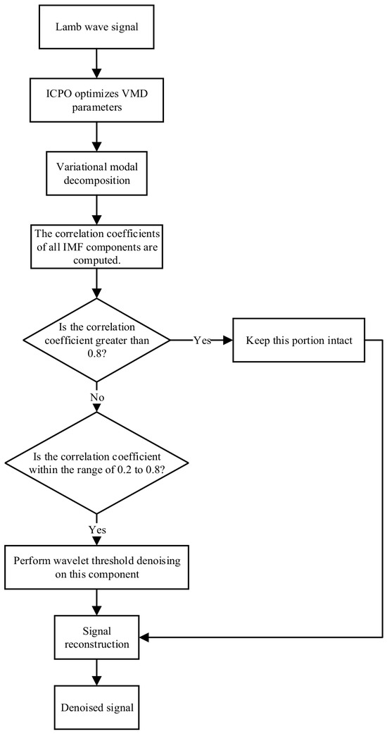
The workflow for wavelet threshold denoising based on the combined improvement of ICPO-VMD is shown in Figure 6:

Figure 6. Flowchart of the ICPO-VMD-based improved wavelet threshold denoising algorithm.

4. Results and Discussion

4.1. Simulated Signal Verification

The performance of the proposed algorithm was first assessed using simulated signals. Combining the physical characteristics of piezoelectric ultrasonic Lamb wave signals, the experiment employed a Gaussian-envelope-modulated sine wave to simulate ultrasonic Lamb wave signals. The mathematical formulation is shown in Equation (34):

$$\mathrm{f}\left(t\right)=A\sin \left(2\pi \mathit{ft}\right)·{\mathrm{e}}^{-{\left({\displaystyle \frac{t-\frac{N}{f}}{\frac{N}{2f}}}\right)}^2}$$

(34)

where A is the amplitude, f is the center frequency, and N is the number of periods.

According to the above expression, the pure simulation signal is designed as shown in Equation (35):

$$\mathrm{f}\left(t\right)=\sin \left(100\pi t\right)·{\mathrm{e}}^{\left[-{\left({\displaystyle \frac{t-0.1}{0.05}}\right)}^2\right]}$$

(35)

Because this signal is obtained through mathematical model simulation, it contains no noise components whatsoever. However, industrial signals are often subject to interference from various noise sources, such as environmental noise and sensor noise. To simulate real operating environments, Gaussian white noise was added to the simulated signal, aiming for a SNR of 10 dB. The simulation serves as a preliminary benchmark to evaluate the basic denoising capability under controlled conditions, while the ultimate purpose lies in experimental measurements that inherently contain realistic noise.

To further validate the stability of the proposed algorithm, both CPO and ICPO were independently run 10 times under identical conditions. The statistical results are summarized in Table 1.

Table 1. Statistical results of CPO and ICPO.

Metric	CPO	ICPO
Mean fuzzy entropy	0.502	0.496
Best value	0.498	0.494
Worst value	0.506	0.500
Standard deviation	0.0027	0.0019
Avg. computational time (s)	22.1	16.2
Orthogonality index	0.0218	0.0197

The results demonstrate that ICPO achieves lower fuzzy entropy values with significantly smaller variance while requiring less computational time compared with CPO. Additionally, the orthogonality index of ICPO is lower than that of CPO, indicating better modal separation.

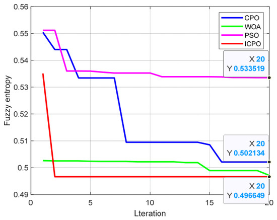
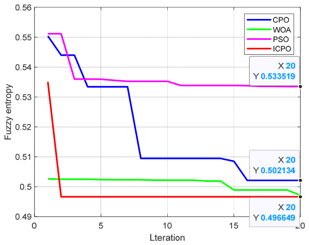
To further validate the superiority of ICPO, a comparison was conducted with two widely used optimization algorithms: particle swarm optimization (PSO) and the whale optimization algorithm (WOA). The convergence curves are shown in Figure 7.

Figure 7. Convergence curves of the four optimization algorithms (simulated signal).

The convergence and statistical comparisons confirm that ICPO achieved the lowest fuzzy entropy (0.496) with the fastest convergence among all compared algorithms.

The superior performance of ICPO can be attributed to its three improvement strategies: dynamic parameter adjustment accelerates convergence, random perturbations help escape local optima, and parallel computing reduces computational time. Accordingly, the optimized parameters derived from ICPO (K = 12, α = 1881) were adopted for subsequent signal decomposition and denoising.

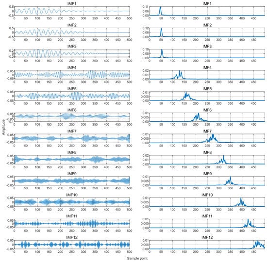
From Figure 8 and Table 2, the spectra and correlation coefficients of each IMF indicate that the decomposed modes exhibit clear separation in the ICPO-VMD decomposition. As listed in Table 2, IMF2 exhibited a correlation coefficient of 0.8093, exceeding the retention threshold of 0.8, indicating that it is dominated by useful signals and can be retained directly. IMF1 and IMF3 yielded coefficients of 0.6617 and 0.6890, respectively, falling within the ambiguous range of 0.2–0.8. To avoid discarding valid information or retaining residual noise, these components were further processed using an improved wavelet threshold denoising method. In contrast, IMF4–IMF12 exhibited coefficients well below 0.2 and were therefore identified as noise-dominated components and discarded.

Figure 8. Waveform and spectrum diagrams of simulated signal decomposition.

Table 2. Correlation coefficients of each IMF component in the simulated signal.

IMF1	IMF2	IMF3	IMF4	IMF5	IMF6	IMF7	IMF8	IMF9	IMF10	IMF11	IMF12
0.6617	0.8093	0.6890	0.0038	0.0023	0.0010	0.0005	0.0003	0.0003	0.0002	0.0002	0.0001

To verify that low-correlation IMFs are noise rather than physically meaningful Lamb wave modes, the dominant frequencies and energy contribution of each IMF were examined in Table 3. IMF1–IMF3 had dominant frequencies of 46 Hz, 50 Hz, and 54 Hz, all matching 50 Hz excitation, with a combined energy contribution of about 92.48%. The remaining IMFs (IMF4–IMF12) had dominant frequencies far above 50 Hz and individual contributions at and below 1.10%. These results confirm that low-correlation components were noise and no physical modes were misclassified. Finally, the denoised signal was obtained by summing the wavelet-denoised IMF1 and IMF3 with the unprocessed IMF2.

Table 3. Dominant frequency and energy contribution of each IMF component in the simulated signal.

IMF	Dominant Frequency	Energy Contribution
IMF1	46	34.77%
IMF2	50	30.76%
IMF3	54	26.95%
IMF4	118	1.03%
IMF5	158	0.75%
IMF6	202	0.70%
IMF7	248	0.97%
IMF8	292	0.58%
IMF9	348	0.79%
IMF10	382	0.79%
IMF11	410	0.80%
IMF12	480	1.10%

To evaluate the performance of the proposed method, a comparison was conducted with the method described earlier. For the proposed method, the db1 wavelet was selected for its suitability in capturing the sharp transient features of the mixed IMF components after VMD decomposition. For standard wavelet thresholding on the whole signal, the coif5 wavelet was adopted, which was selected through preliminary experiments as the best-performing wavelet. The decomposition level of both methods is 3.

SNR and RMSE were simultaneously introduced to evaluate the denoised signal. SNR measures the strength relationship between the desired signal and noise components, and RMSE reflects the overall difference between the denoised signal and the original signal. Their definitions are expressed as Equations (36) and (37), where $x\left(n\right)$ denotes the original signal and$\hat{x}\left(n\right)$ represents the denoised signal, with N representing the length of the signal.

$$\mathrm{SNR}=10{\log }_{10}\left({\displaystyle \frac{{\sum }_{n=1}^N{\left[x\left(n\right)\right]}^2}{{\sum }_{n=1}^N{\left[x\left(n\right)-\hat{x}\left(n\right)\right]}^2}}\right)$$

(36)

$$\mathrm{RMSE}=\sqrt{{\displaystyle \frac{1}{N}}{\displaystyle \sum _{n=1}^N}{\left[x\left(n\right)-\hat{x}\left(n\right)\right]}^2}$$

(37)

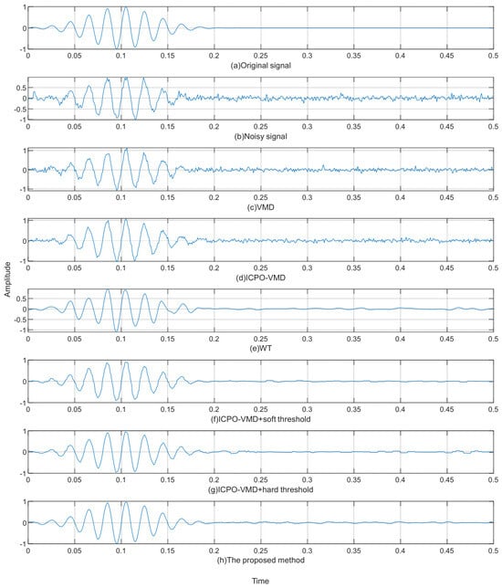
Figure 9 shows the denoising results of the six methods. Compared with VMD (Figure 9c), ICPO-VMD (Figure 9d) provided a slight improvement but still retained some noise. Direct WT denoising on the whole signal (Figure 9e) smoothed the waveform but introduced signal distortion. In contrast, applying wavelet thresholding only to the mixed IMF components after ICPO-VMD decomposition (Figure 9f–h) achieved better detail preservation. The proposed method (Figure 9h) produced the best reconstruction, effectively removing noise while maintaining the signal envelope and peak structure.

Figure 9. Waveform diagrams of simulated signals after noise reduction using six methods.

These visual observations were further corroborated by quantitative evaluation metrics.

Table 4 shows that ICPO-VMD combined with improved wavelet threshold denoising yielded a higher SNR of 20.246 dB and a lower RMSE of 0.0244. This demonstrates that the proposed method effectively enhances signal quality while mitigating noise interference.

Table 4. SNR and RMSE of simulated signals after noise reduction using six methods.

Method/Signal Type	SNR	RMSE
Noisy signal	10	—
VMD	11.354	0.0671
ICPO-VMD	12.095	0.0626
WT	13.827	0.0550
ICPO-VMD + soft threshold	17.468	0.0335
ICPO-VMD + hard threshold	19.182	0.0273
The proposed method	20.246	0.0244

The superior performance of ICPO can be attributed to its three improvement strategies: dynamic parameter adjustment accelerates convergence, random perturbation helps escape local optima, and parallel computing reduces computational time. As shown in Figure 7, ICPO achieved the fastest convergence among all compared algorithms, reaching the optimal solution within approximately five iterations. The statistical results in Table 1 confirm that ICPO consistently obtained lower fuzzy entropy with smaller variance, while the parallel implementation reduced the average processing time from 22.1 s to 16.2 s. A sensitivity analysis confirmed that the algorithm maintained stable performance under reasonable parameter variations.

Furthermore, compared with direct WT denoising and ICPO-VMD combined with soft or hard thresholding, the proposed method achieved better denoising performance by applying improved wavelet thresholding more effectively to the mixed IMF components. Compared to the traditional VMD algorithm, the ICPO-VMD combined with improved wavelet threshold denoising achieved a 78.3% increase in the SNR of the simulated signal and a 63.6% reduction in the RMSE. These improvements were calculated as ${\displaystyle \frac{\mathrm{Value}\text{\_}\mathrm{Proposed}-\mathrm{Value}\text{\_}\mathrm{VMD}}{\mathrm{Value}\text{\_}\mathrm{VMD}}}\times 100\%$. These results demonstrate the effectiveness, robustness, and efficiency of the proposed method for Lamb wave signal denoising.

4.2. Measured Signal Verification

To further substantiate the operational viability of the proposed algorithm, it was implemented in the experimental process of piezoelectric ultrasonic non-destructive testing. The experimental apparatus consisted of a 1000 mm × 1000 mm × 1 mm aluminum plate, a function generator, a power amplifier, a preamplifier, an oscilloscope, piezoelectric sensors, and connecting wires. Eight sensors were arranged on the plate surface in a 3 × 3 grid pattern with adjacent spacing of 50 mm. A 200 kHz sinusoidal excitation signal with an amplitude of 200 mV was generated by a function generator, amplified by a power amplifier, and applied to the transmitting sensor to generate Lamb waves. The propagated signals were captured by the receiving sensors, amplified by a preamplifier, and recorded by an oscilloscope with a sampling interval of 0.4 μs. After acquisition, the signals were transferred to MATLAB for denoising using the proposed algorithm.

For the measured signals, each signal was recorded three times. The results showed negligible differences among the repetitions, confirming the consistency of the measurements. Based on this, the formal experiments were then carried out according to the procedure described below.

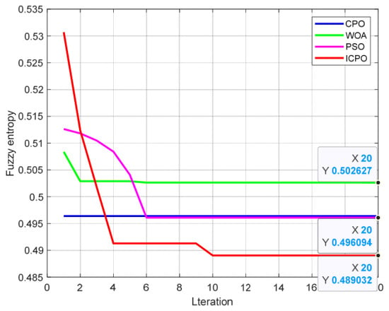
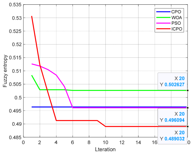
Figure 10 confirms that ICPO achieved the lowest fuzzy entropy with the fastest convergence among all compared algorithms on the measured signal. The average computational time of ICPO was 31.4 s, compared with 40.8 s for CPO. These results demonstrate its effectiveness in accelerating global convergence and escaping local optima in practical detection environments. Therefore, the optimal parameters identified by the ICPO algorithm (K = 6, α = 2475) were selected for this experiment.

Figure 10. Convergence curves of the four optimization algorithms (measured signal).

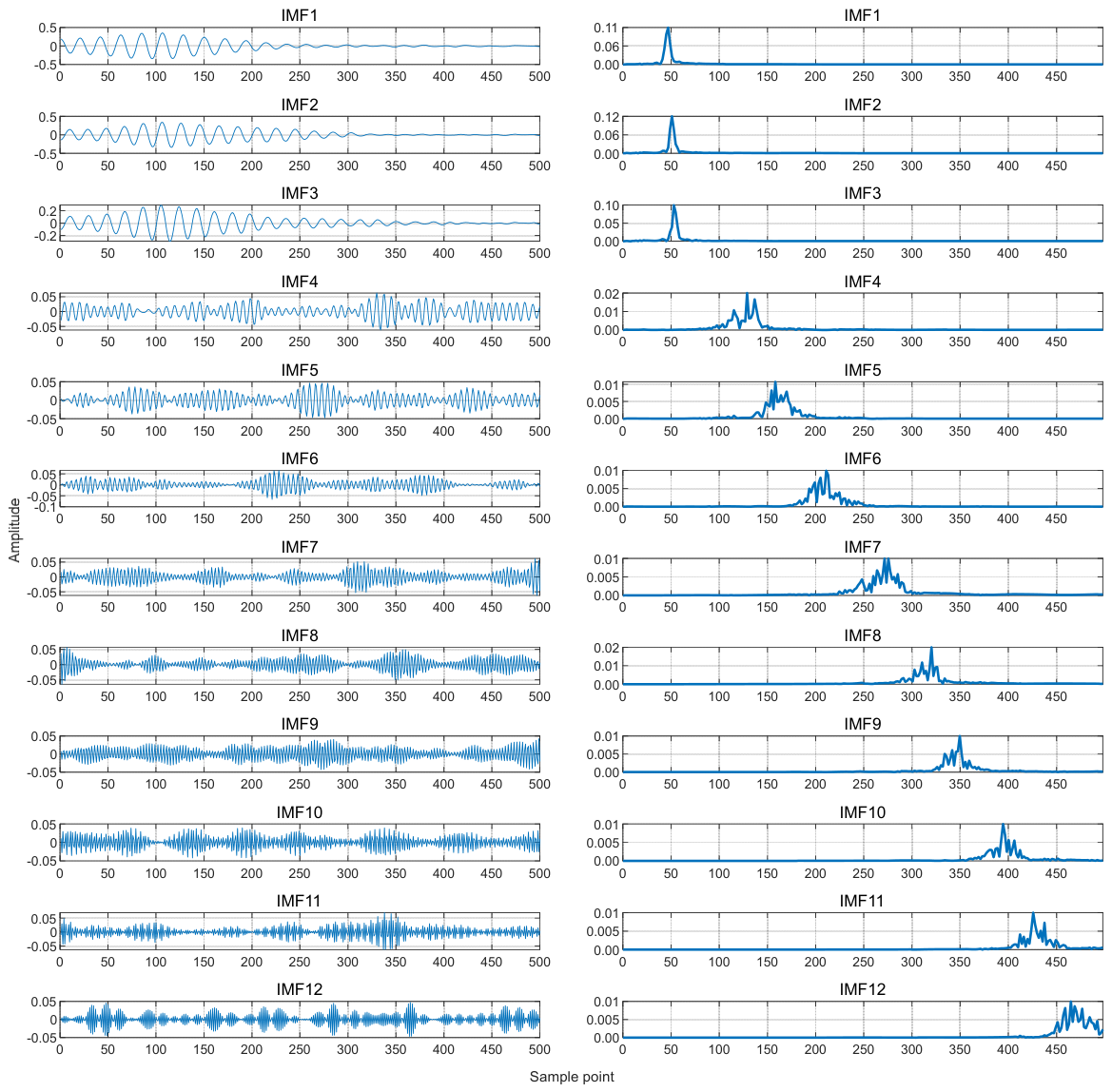
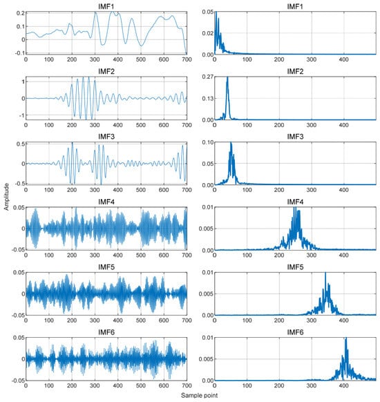
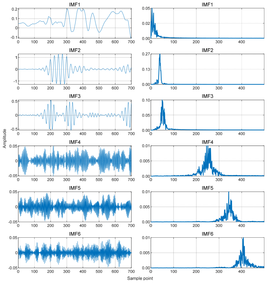
As illustrated in Figure 11 and Table 5, the ICPO-optimized VMD algorithm effectively decomposed the measured signal into low-frequency smooth components and high-frequency noisy components. IMF2 yielded a correlation coefficient of 0.9094 and was therefore retained directly. In contrast, IMF1 and IMF3 exhibited correlation coefficients within the range of 0.2–0.8 and were therefore subjected to the improved wavelet threshold denoising procedure. The reconstructed denoised signal can be generated by combining the processed IMF1 and IMF3 with the unmodified IMF2. To evaluate the method’s efficacy on real-world signals, further comparative experiments were conducted, in which the wavelet decomposition level was fixed at three, and the mother wavelet was set to ‘db1’.

Figure 11. Waveform and spectrum diagram of the decomposed measured signal.

Table 5. Correlation coefficients of each IMF component in the measured signal.

IMF1	IMF2	IMF3	IMF4	IMF5	IMF6
0.2524	0.9094	0.5100	0.0310	0.0209	0.0222

Since pure signals cannot be obtained in practice, SNR and RMSE are no longer applicable as evaluation metrics. To comprehensively evaluate the denoising performance on the measured signals, this paper combined the energy retention ratio (ERR), residual variation rate (RVR), and the normalized cross-correlation coefficient (NCC). The ERR represents the ratio of the total energy of the denoised signal to the total energy of the original signal, as shown in Equation (38). A value closer to 1 indicates better energy preservation during denoising. The RVR is used to assess the smoothness of the denoised signal, as shown in Equation (39). A RVR closer to zero indicates higher signal smoothness, while pure and effective Lamb wave signals are relatively smooth. Additionally, the NCC is introduced to evaluate the waveform similarity between the denoised signal and the original signal, as defined in Equation (40). Its value ranges from 0 to 1, with a value closer to 1 indicating better waveform preservation and less distortion. Therefore, through a comprehensive analysis of these three metrics with waveform comparisons, the effectiveness of the denoising algorithm can be fully evaluated.

$$\mathrm{ERR}={\displaystyle \frac{{\sum }_{i=1}^N{{\hat{x}}_i}^2}{{\sum }_{i=1}^N{x_i}^2}}$$

(38)

$$\mathrm{RVR}={\displaystyle \frac{{\displaystyle {\sum }_{i=1}^{N-1}}{\left[{\hat{x}}_{i+1}-{\hat{x}}_i\right]}^2}{{\displaystyle {\sum }_{i=1}^N}{{\hat{x}}_i}^2}}$$

(39)

$$\mathrm{NCC}={\displaystyle \frac{{\sum }_{i=1}^N\left(x_i-\overline{x}\right)\left({\hat{x}}_i-\overline{\hat{x}}\right)}{\sqrt{{\sum }_{i=1}^N{\left(x_i-\overline{x}\right)}^2}\sqrt{{\sum }_{i=1}^N{\left({\hat{x}}_i-\overline{\hat{x}}\right)}^2}}}$$

(40)

where$x_i$denotes the original signal,${\hat{x}}_i$denotes the denoised signal, $N$is the signal length, and$\stackrel{\mathrm{-}}{x}$ and$\overline{\hat{x}}$ are the mean values of the original and denoised signals, respectively.

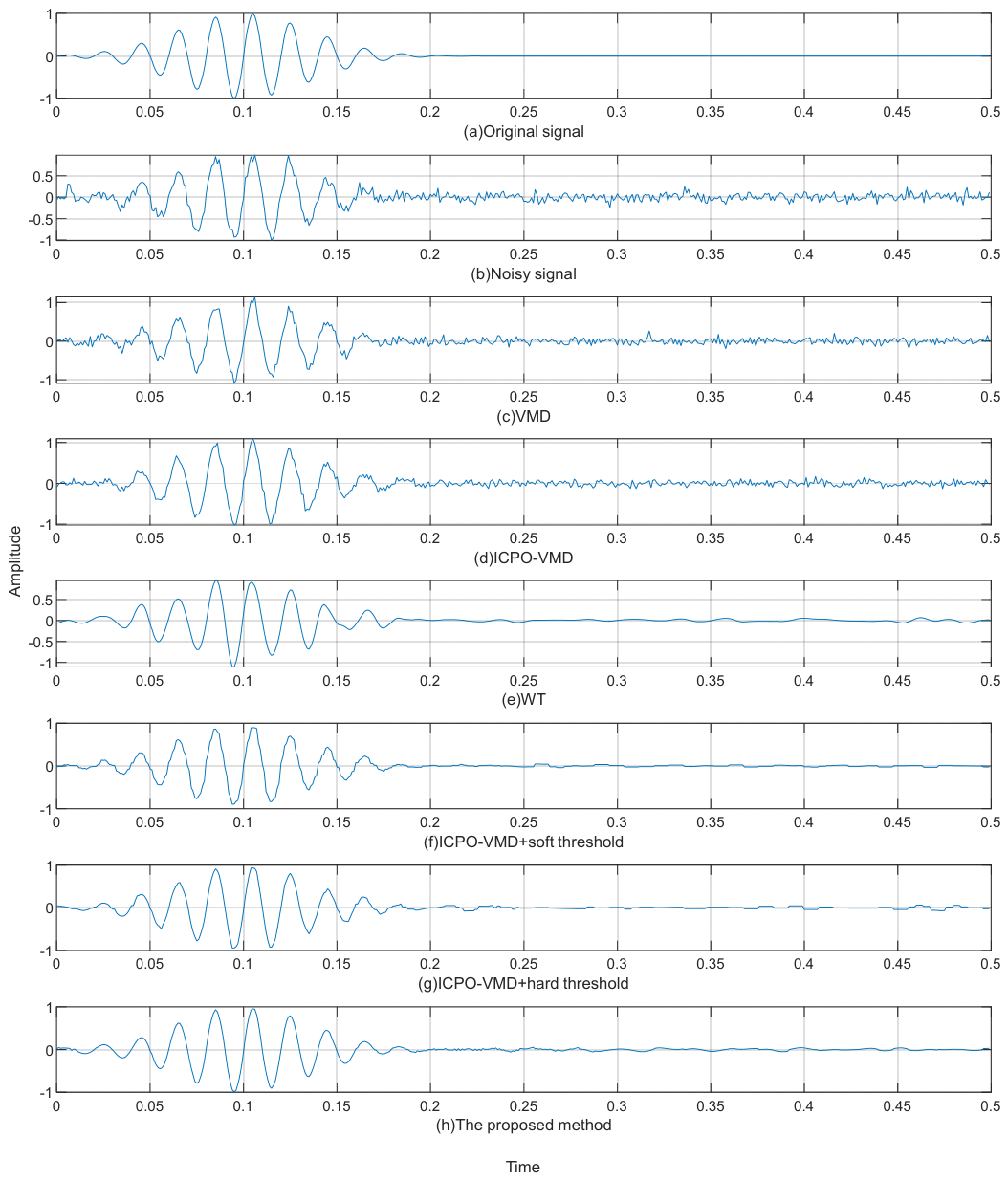
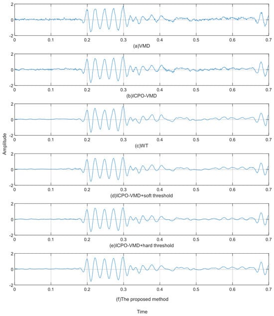
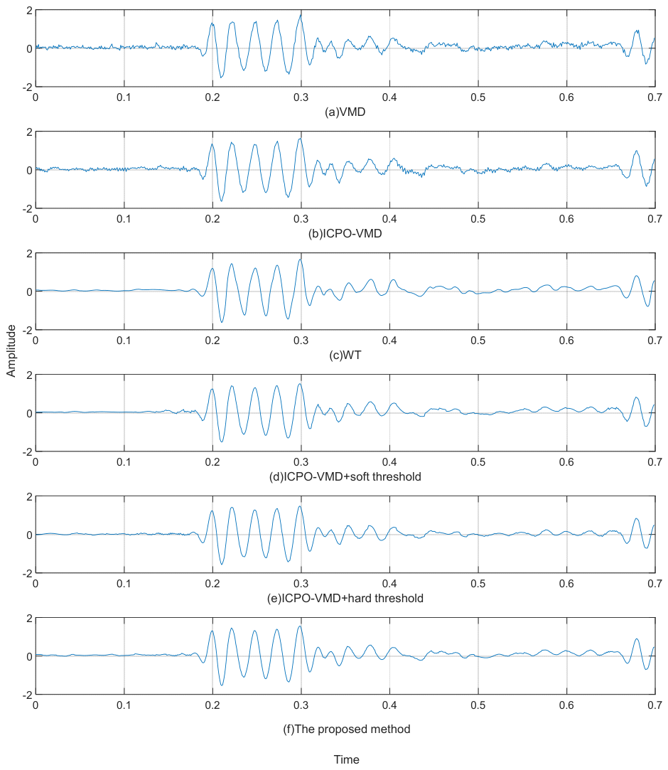
Figure 12 shows the denoising results on the measured signal. The proposed method achieved the best reconstruction among all compared methods, outperforming VMD, WT, and ICPO-VMD combined with soft or hard thresholding, which is consistent with the simulation results.

Figure 12. Waveform diagrams of the measured signals after noise reduction using six methods.

Quantitative assessments of the denoised measured signals are summarized in Table 6. Compared with direct WT denoising and ICPO-VMD combined with soft or hard thresholding, the proposed method achieved better removal of noise components that were unrelated to the main signal structure. Compared with the conventional VMD algorithm, the proposed method achieved a 5.96% increase in ERR, an 11.5% increase in NCC, and a 38.8% reduction in RVR. These results confirm that the proposed method effectively preserves the basic signal content and promotes smoother and more reliable signal reconstruction.

Table 6. ERR, RVR, and NCC after noise reduction of the measured signals using six methods.

Method	ERR	RVR	NCC
VMD	0.8678	0.1084	0.8853
ICPO-VMD	0.8602	0.0994	0.9255
WT	0.9086	0.0702	0.9183
ICPO-VMD + soft threshold	0.9021	0.0782	0.9746
ICPO-VMD + hard threshold	0.9127	0.0736	0.9789
The proposed method	0.9195	0.0663	0.9871

Overall, the superior denoising performance of the proposed method can be attributed to two key factors: ICPO-based VMD parameter optimization and the improved wavelet threshold function. The ICPO algorithm ensures that the VMD decomposition captures the main signal components with minimal mode mixing, while the improved wavelet threshold function effectively removes residual noise from the mixed modes without introducing the bias or discontinuity inherent in conventional soft or hard thresholding. Therefore, the proposed method demonstrates strong feasibility and practical potential in denoising aluminum plate Lamb wave signals for nondestructive testing applications, although its performance may be limited when dealing with significantly different experimental conditions, such as other plate materials or thicknesses, which remain to be further investigated.

5. Conclusions

To overcome the effect of industrial interference that can easily overwhelm useful information in ultrasonic Lamb wave signals, an integrated processing framework combining ICPO-VMD with an enhanced wavelet threshold denoising technique was developed. Through simulation and experimental verification, the following conclusions were drawn:

• To eliminate the subjectivity in selecting the mode number K and penalty factor α for VMD, as well as to address the limited adaptability of the standard CPO algorithm, this study adopted the ICPO algorithm to optimize VMD parameters, utilizing fuzzy entropy as the fitness function. Experimental results demonstrate that ICPO outperformed CPO in terms of both optimization efficiency and mode purity under both simulated and measured signal conditions.
• To address the shortcomings of both soft and hard wavelet threshold methods, an improved wavelet threshold denoising algorithm was introduced. It applies denoising to the mixed modes extracted by VMD decomposition. Results from the experiments confirm that the proposed wavelet thresholding approach achieved better denoising performance than conventional soft and hard threshold methods for the Lamb wave signals tested in this study.
• Through simulation and experimental verification, compared to the traditional VMD algorithm, the ICPO-VMD combined with improved wavelet threshold denoising achieved a 78.3% increase in SNR and a 63.6% reduction in RMSE on simulated signals. For measured signals, it achieved a 5.96% increase in ERR, an 11.5% increase in NCC, and a 38.8% reduction in RVR. These results indicate that the proposed method effectively suppresses noise while preserving signal characteristics, demonstrating strong feasibility and practical potential for aluminum plate Lamb wave denoising applications under the tested conditions.

References

- Teng, F.; Zhang, H.; Lv, S.; Zhang, L.; Zhang, F.; Jiang, M. Improved-probabilistic imaging algorithm for separation problem of helical scattered path in pipeline ultrasonic guided wave inspection. Measurement 2025, 253, 117474. [Google Scholar] [CrossRef] [Scilit]
- Han, B.; Omer, A.M.; Shao, T.; He, L.; Ding, X.; Long, Z.; Fu, J.; Zhang, H.; Duan, Y. A Quantitative Review of Air-Coupled Ultrasonic Lamb Wave Analysis Based on Signal Transformations. Russ. J. Nondestruct. Test. 2024, 60, 157–169. [Google Scholar] [CrossRef] [Scilit]
- Lu, H.; Chandran, B.; Wu, W.; Ninic, J.; Gryllias, K.; Chronopoulos, D. Damage Features for Structural Health Monitoring Based on Ultrasonic Lamb Waves: Evaluation Criteria, Survey of Recent Work and Outlook. Measurement 2024, 232, 114666. [Google Scholar] [CrossRef] [Scilit]
- Mirahmadi, S.J.; Honarvar, F. Application of Signal Processing Techniques to Ultrasonic Testing of Plates by S0 Lamb Wave Mode. NDT E Int. 2011, 44, 131–137. [Google Scholar] [CrossRef] [Scilit]
- Xu, H.; Liu, L.; Li, X.; Xiang, Y.; Xuan, F.-Z. Wavefield Imaging of Nonlinear Ultrasonic Lamb Waves for Visualizing Fatigue Micro-Cracks. Ultrasonics 2024, 138, 107214. [Google Scholar] [CrossRef] [Scilit] [PubMed]
- Chen, Y.; Wang, G.; Li, Z. Study of Lamb Wave Hybrid Imaging Technology in High Noise Environments. Wave Motion 2025, 138, 103548. [Google Scholar] [CrossRef] [Scilit]
- Zhou, J.; Peng, Y.; Shao, H.; Shen, Y.; Bin, G.; Zheng, J.; Pan, H.; Xu, Y. Empirical Fourier–Bessel Heuristic Denoising and Its Application to Gear Fault Diagnosis. ISA Trans. 2025, 167, 1906–1924. [Google Scholar] [CrossRef] [Scilit] [PubMed]
- Liu, J.; Zhang, Q.; Li, D.; Teng, Y.; Wu, S.; Wang, X. A Parameter-Adaptive Spectral Graph Wavelet Transform Method for Wind Turbines Vibration Signal Denoising. Int. J. Mech. Sci. 2024, 270, 109075. [Google Scholar] [CrossRef] [Scilit]
- Ma, H.-W.; Fan, H.-W.; Mao, Q.-H.; Zhang, X.-H.; Xing, W. Noise Reduction of Steel Cord Conveyor Belt Defect Electromagnetic Signal by Combined Use of Improved Wavelet and EMD. Algorithms 2016, 9, 62. [Google Scholar] [CrossRef] [Scilit]
- Wang, K.; Xu, Z.-J.; Gong, Y.; Du, K.-L. Mechanical Fault Prognosis through Spectral Analysis of Vibration Signals. Algorithms 2022, 15, 94. [Google Scholar] [CrossRef] [Scilit]
- Huang, N.E.; Shen, Z.; Long, S.R.; Wu, M.C.; Shih, H.H.; Zheng, Q.; Yen, N.-C.; Tung, C.C.; Liu, H.H. The Empirical Mode Decomposition and the Hilbert Spectrum for Nonlinear and Non-Stationary Time Series Analysis. Proc. R. Soc. A 1998, 454, 903–995. [Google Scholar] [CrossRef] [Scilit]
- White, A.; Hong, J.W.; Hong, S.; Choi, J. Parameter Estimation for Wavelet Transformed Ultrasonic Signals. NDT E Int. 2011, 44, 32–40. [Google Scholar] [CrossRef] [Scilit]
- Zhang, J.; Chen, J.; Pan, J.; Ji, Z.; Yang, G.; Xia, Y. An Adaptive Denoising Method Based on ICEEMDAN–EKWSTD for Cutter Rotational Speed Signals in Tunnel Boring Machines. Measurement 2026, 265, 120412. [Google Scholar] [CrossRef] [Scilit]
- Guo, C.; Wen, Y.; Li, P.; Wen, J. Adaptive Noise Cancellation Based on EMD in Water-Supply Pipeline Leak Detection. Measurement 2016, 79, 188–197. [Google Scholar] [CrossRef] [Scilit]
- Zhou, Y.; Ma, Z.; Fu, L. A Review of Key Signal Processing Techniques for Structural Health Monitoring: Highlighting Non-Parametric Time-Frequency Analysis, Adaptive Decomposition, and Deconvolution. Algorithms 2025, 18, 318. [Google Scholar] [CrossRef] [Scilit]
- Dragomiretskiy, K.; Zosso, D. Variational Mode Decomposition. IEEE Trans. Signal Process. 2014, 62, 531–544. [Google Scholar] [CrossRef] [Scilit]
- Zhou, X.; Wang, X.; Wang, H.; Xing, Z.; Yang, Z.; Cao, L. Method for Denoising the Vibration Signal of Rotating Machinery through VMD and MODWPT. Sensors 2023, 23, 6904. [Google Scholar] [CrossRef] [Scilit] [PubMed]
- Wang, Y.; Wang, D.; Chi, C.; Yu, Z.; Li, J.; Yu, L. Ship Shaft-Rate Electric Field Signal Denoising Method Based on VMD-MSS. J. Mar. Sci. Eng. 2024, 12, 544. [Google Scholar] [CrossRef] [Scilit]
- Wang, Y.; Zhang, S.; Cao, R.; Xu, D.; Fan, Y. A Rolling Bearing Fault Diagnosis Method Based on the WOA-VMD and the GAT. Entropy 2023, 25, 889. [Google Scholar] [CrossRef] [Scilit] [PubMed]
- Hu, Z.; Zhang, R.; Li, R.; Li, Y.; Yan, X.; Qian, C.; Han, G. A Vibration Signal Processing Method of Wind Turbine Gearbox Based on Fiber Grating and GWO-VMD Algorithm. In Proceedings of the 2025 7th International Academic Exchange Conference on Science and Technology Innovation (IAECST), Guangzhou, China, 26–28 December 2025; pp. 1117–1124. [Google Scholar] [CrossRef] [Scilit]
- Abdel-Basset, M.; Mohamed, R.; Abouhawwash, M. Crested Porcupine Optimizer: A New Nature-Inspired Metaheuristic. Knowl. -Based Syst. 2024, 284, 111257. [Google Scholar] [CrossRef] [Scilit]
- Lin, M.; Dai, Z.; Qiu, Z.; Wang, Y.; Chen, H. Multi-strategy enhanced sand cat swarm optimization algorithm and its engineering applications. Sci. Rep. 2025, 15, 34391. [Google Scholar] [CrossRef] [Scilit] [PubMed]
- Xie, H.-B.; Sivakumar, B.; Boonstra, T.W.; Mengersen, K. Fuzzy Entropy and Its Application for Enhanced Subspace Filtering. IEEE Trans. Fuzzy Syst. 2018, 26, 1970–1982. [Google Scholar] [CrossRef] [Scilit]
- Zhou, Y.; Cao, H.; Guo, T. A Hybrid Algorithm for Noise Suppression of MEMS Accelerometer Based on the Improved VMD and TFPF. Micromachines 2022, 13, 891. [Google Scholar] [CrossRef] [Scilit] [PubMed]
- Jia, G.; Yang, J.; Liang, H. A Combined Denoising Method of Adaptive VMD and Wavelet Threshold for Gear Health Monitoring. Struct. Durab. Health Monit. 2025, 19, 105772. [Google Scholar] [CrossRef] [Scilit]
- Guo, J.; Si, Z.; Xiang, J. A Compound Fault Diagnosis Method of Rolling Bearing Based on Wavelet Scattering Transform and Improved Soft Threshold Denoising Algorithm. Measurement 2022, 196, 111276. [Google Scholar] [CrossRef] [Scilit]
- Cheng, L.; Zhang, S.; Qi, Z.; Wang, X.; Chen, Y.; Feng, P. Research on eLoran Weak Signal Extraction Based on Wavelet Hard Thresholding Processing. Remote Sens. 2024, 16, 3012. [Google Scholar] [CrossRef] [Scilit]
- Li, S.; Zhu, X.; Zhou, D. Power Quality Disturbance Signal Denoising and Detection Based on Improved DBO-VMD Combined with Wavelet Thresholding. Electr. Power Syst. Res. 2025, 238, 111193. [Google Scholar] [CrossRef] [Scilit]
- Xu, J.; Ma, H.; He, W. Harmonic Detection Method Based on Parameter Optimization VMD-IWT Combined Noise Reduction. Appl. Sci. 2024, 14, 5076. [Google Scholar] [CrossRef] [Scilit]
Disclaimer/Publisher’s Note: The statements, opinions and data contained in all publications are solely those of the individual author(s) and contributor(s) and not of MDPI and/or the editor(s). MDPI and/or the editor(s) disclaim responsibility for any injury to people or property resulting from any ideas, methods, instructions or products referred to in the content. |
© 2026 by the authors. Licensee MDPI, Basel, Switzerland. This article is an open access article distributed under the terms and conditions of the Creative Commons Attribution (CC BY) license.