Computational Modeling and Intelligent Simulation of PEMFC Parameter Identification: Design and Technical Validation of a Virtual Teaching Experiment Using an Enhanced LRSAO Algorithm

Abstract

Proton exchange membrane fuel cell (PEMFC) parameter identification is a nonlinear computational modeling problem involving strongly coupled electrochemical parameters and partially unobservable polarization processes. Its experimental teaching is further constrained by the cost of fuel cell stacks and the safety requirements associated with hydrogen operation. To address these challenges, this study develops a computational modeling and intelligent simulation framework for a virtual teaching experiment on PEMFC parameter identification. A semi-empirical output-voltage model is established, and the sum of squared errors (SSE) between measured and simulated voltages is formulated as the optimization objective. An enhanced Logistic–Tent reverse snow ablation optimizer (LRSAO), termed RLFDB-LRSAO, is introduced by integrating roulette-wheel-selection-enhanced fitness-distance balance and Lévy flight perturbation. Its methodological novelty lies in the stage-wise coordination of population-diversity enhancement, candidate-selection guidance, and search perturbation within the LRSAO framework, rather than in the individual component strategies themselves. The framework organizes the identification process into mechanism interpretation, model construction, algorithm implementation, parameter configuration, visualization, comparative evaluation, and reflective analysis. Case studies using the NedStack PS6 and Modular SR-12 stacks yield best SSE values of 1.2173340 and 6.13503904, respectively. A small-scale qualitative teaching evaluation involving 20 postgraduate students indicated that the framework supported programming practice, strengthened conceptual understanding of PEMFC parameter identification and intelligent optimization, and provided useful support for research-oriented skills such as engineering problem analysis, technical writing, and innovation-oriented project development. These results provide preliminary evidence of technical and educational feasibility while supporting a cautious, problem-dependent interpretation of the optimizer.

1. Introduction

Proton exchange membrane fuel cell (PEMFC) parameter identification provides a demanding but instructive setting in which learners must connect an engineering mechanism, a mathematical model, an objective function, and a numerical search procedure. Computational parameter estimation studies commonly organize this process around model formulation, objective function construction, numerical optimization, and performance comparison [1]. Virtual and immersive learning environments can make otherwise inaccessible processes repeatable and observable [2]. Hybrid optimization strategies have also been applied to engineering parameter prediction problems [3], while virtual laboratory research demonstrates the value of repeatable simulation-based learning in engineering education [4]. Enhanced sampling strategies can further provide useful mechanisms for comparing global and local search behavior [5]. The educational problem addressed here is therefore not visualization alone but the transformation of a nonlinear identification workflow into a transparent and reproducible learning task.

The continuing expansion of the global hydrogen sector further increases the demand for engineering education in fuel cell modeling and intelligent optimization. According to the International Energy Agency, global hydrogen demand grew by almost 3% in 2025 and surpassed 100 million tonnes, while low-emissions hydrogen production increased by approximately 20% to almost 1 million tonnes but still accounted for less than 1% of global production [6]. At the same time, recent multi-stack PEMFC studies show that parameter identification remains a nonlinear and computationally demanding problem requiring accuracy, robustness, and statistical evaluation [7], while digital-twin research illustrates the growing role of model-based analysis in fuel cell operation and lifetime management [8]. Direct stack testing, however, involves equipment cost, hydrogen-safety requirements, restricted operating conditions, and limited opportunities for repeated algorithmic trials.

The educational design must go beyond a prepared demonstration. Authentic engineering problems are often ill-structured and require learners to connect theory, modeling, experimentation, and interpretation [9]. Practice-oriented curricula likewise emphasize active model construction and iterative decision-making [10]. Li and Liang [11] synthesized 46 independent studies from 22 publications and reported a moderate positive overall effect of virtual laboratories on engineering-education outcomes (Hedges’ g was 0.686, 95% CI: 0.414–0.959). Their analysis further showed particularly strong effects on learning motivation and engagement and indicated that virtual laboratories are better positioned as a complement to, rather than a complete replacement for, hands-on laboratory activities. A fuel cell-specific virtual simulation tool has also been developed for performance-testing instruction [12], but its emphasis is mainly on system structure, operation, and performance testing rather than algorithm-transparent parameter identification. Reviews of artificial intelligence in higher education further stress the importance of explicit pedagogical design and educator involvement [13].

Semi-empirical PEMFC models are widely used for parameter estimation because they retain interpretable voltage-loss terms while remaining computationally manageable [14]. Recent optimizer-based studies continue to improve numerical extraction of the seven unknown parameters [15]. Zhou et al. [16] proposed an improved snow ablation optimizer (SAO) that combines subgroup cooperative optimization, learning-automata-based adaptive dimension assignment, and a t-distribution-based adaptive step-size mechanism to alleviate cross-dimensional interference and improve the balance between exploration and exploitation in high-dimensional optimization. Liu et al. [17] developed an improved SAO by integrating a normal cloud model and a Cauchy mutation mechanism, thereby strengthening the algorithm’s ability to escape local optima. Kumari et al. [18] applied SAO to a multi-objective bi-level planning problem for electric-vehicle-based energy storage systems, demonstrating the flexibility of the algorithm in complex engineering optimization. Nevertheless, the original SAO still relies on relatively simple random population initialization and search-guidance mechanisms and may suffer from insufficient population diversity, premature convergence, and an inadequate balance between global exploration and local exploitation. To address these limitations in PEMFC parameter identification, the present study introduces Logistic–Tent chaotic mapping and elite opposition-based learning to improve initial population diversity, incorporates roulette wheel-selection-enhanced fitness-distance balance (RFDB) to strengthen candidate-selection guidance, and employs Lévy flight perturbation to enhance the ability to escape locally concentrated search regions. Related work from the authors’ group has addressed PEMFC degradation prediction, remaining-useful-life prediction, and semi-empirical parameter identification [19,20,21]. These studies provide a computational foundation, but research-oriented algorithms must be reorganized before they can function as teachable, inspectable, and assessable learning activities.

Existing fuel cell simulation and parameter identification studies therefore leave a specific gap: virtual teaching tools commonly emphasize operating principles or performance testing, whereas optimization studies emphasize the lowest numerical error. The aim of this work is to connect these two directions by developing a teaching-oriented virtual simulation framework in which learners can inspect the PEMFC model, objective function, optimization modules, code structure, and evaluation criteria. The contributions are as follows:

(1) A teaching-oriented semi-empirical PEMFC parameter identification framework is developed by reorganizing the voltage model into mechanism analysis, mathematical formulation, parameter interpretation, and objective function construction. This structure helps learners understand the relationship between physical mechanisms, model parameters, and identification objectives.

(2) An enhanced RLFDB-LRSAO algorithm is developed by integrating Logistic–Tent chaotic mapping, elite opposition-based learning, RFDB, and Lévy flight perturbation. These strategies are introduced to improve population diversity, search guidance, and the balance between global exploration and local exploitation.

(3) A structured virtual simulation teaching framework is established using MATLAB-based modular code, process-oriented tasks, and result visualization. The design aims to reduce black box operation and strengthen students’ understanding of model construction, algorithm implementation, and result interpretation.

(4) The proposed framework is evaluated through two PEMFC parameter identification cases, a six-function ablation study, and nonparametric statistical comparison. A small-scale qualitative pilot involving postgraduate students further provides preliminary evidence of its educational applicability and research-training value.

The remainder of this paper is organized as follows. Section 2 presents the teaching-oriented semi-empirical PEMFC parameter identification model, including the working principle, mathematical formulation, objective function, parameter interpretation, and model limitations. Section 3 describes the improved intelligent optimization algorithm and the development of RLFDB-LRSAO. Section 4 introduces the virtual simulation teaching design, including the experimental process, software environment, process-oriented assessment, and hierarchical learning design. Section 5 reports the PEMFC case studies, comparative experiments, ablation analysis, statistical evaluation, computational cost analysis, and preliminary qualitative teaching evaluation. Finally, Section 6 summarizes the main conclusions and discusses the implications and future directions of the proposed framework.

2. Teaching-Oriented PEMFC Parameter Identification Model

2.1. Working Principle of PEMFCs

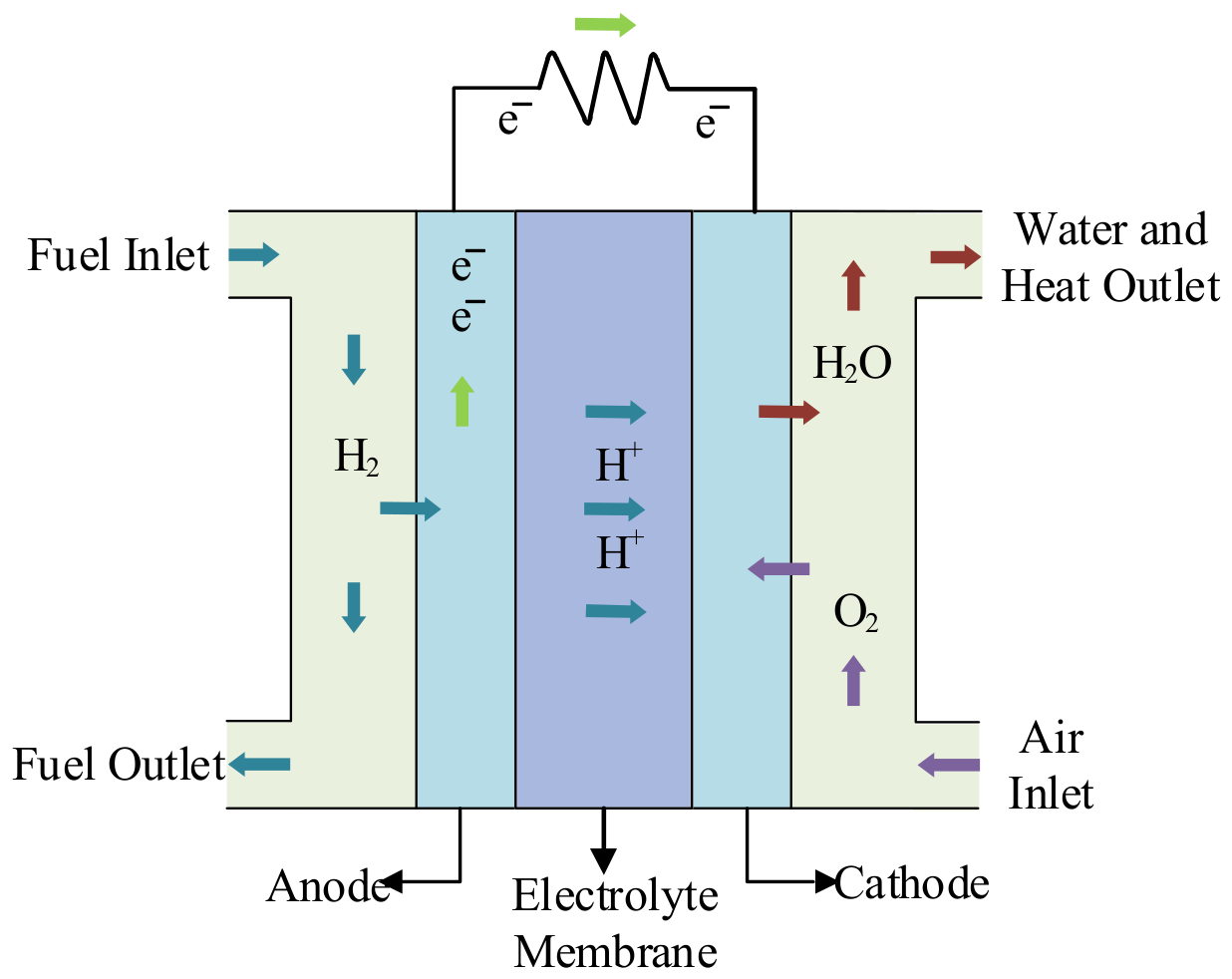
A PEMFC stack generates electricity through coupled electrochemical reactions at the anode and cathode. During operation, hydrogen is introduced into the anode channel and dissociates into protons and electrons on the catalyst surface. The protons migrate across the proton exchange membrane to the cathode, whereas the electrons are forced to pass through the external circuit and deliver electrical work to the load. On the cathode side, oxygen reacts with the transported protons and external-circuit electrons, producing water and heat. This operating process explains why the stack voltage is closely related to current density, reactant partial pressure, membrane hydration, and temperature. Figure 1 illustrates the PEMFC working mechanism used for classroom explanation.

The corresponding anode reaction and overall reaction are expressed as follows:

$$H_2\to 2H^{+}+2e^{-}$$

(1)

$$4H^{+}+4e^{-}+O_2\to 2H_{2}O$$

(2)

Hydrogen is oxidized at the anode to generate protons and electrons, whereas oxygen reacts with the transported protons and external-circuit electrons at the cathode to produce water. The external electron pathway supplies electrical power to the load.

2.2. Semi-Empirical Output Model and Objective Function

For teaching implementation, a semi-empirical voltage model is more suitable than a purely microscopic model because it keeps the physical meaning of the key losses while remaining computationally feasible for students [22]. The single-cell output voltage is written as

$$V_C=E_{\mathrm{N}\mathrm{e}\mathrm{r}\mathrm{n}\mathrm{s}\mathrm{t}}-V_{\mathrm{C}\mathrm{O}}-V_o-V_a$$

(3)

where V_c is the single-cell output voltage, E_Nernst is the thermodynamic electromotive force, and V_CO, V_o and V_a denote the concentration-polarization, ohmic-polarization and activation polarization overvoltages, respectively. In Equations (4) and (5), T is the operating temperature of the PEMFC stack in K; P_H2 and P_O2 are the partial pressures of hydrogen and oxygen in bar; J is the current density; J_MAX is the maximum allowable current density; and b is a cell-state-related parameter to be identified. The reversible voltage and concentration-polarization loss are calculated by

$$E_{\mathrm{N}\mathrm{e}\mathrm{r}\mathrm{n}\mathrm{s}\mathrm{t}}=1.229-0.85\times {10}^{-5}\left(T-298.15\right)+4.3085\times {10}^{-5}T\left(\mathrm{l}\mathrm{n}{P}_{H2}+{\displaystyle \frac{\mathrm{l}\mathrm{n}{P}_{O2}}{2}}\right)$$

(4)

$$V_{\mathrm{C}\mathrm{O}}=-b\mathrm{l}\mathrm{n}\left(1-{\displaystyle \frac{J}{J_{\mathrm{M}\mathrm{A}\mathrm{X}}}}\right)$$

(5)

where I is the PEMFC output current, R_C is the equivalent contact resistance to be identified, and R_F is the equivalent proton exchange membrane resistance. The ohmic loss and membrane resistance are given by

$$V_o=I\left(R_F+R_C\right)$$

(6)

$$R_F={\rho }_F{\displaystyle \frac{L}{A}}$$

(7)

$${\rho }_F={\displaystyle \frac{181.6\left[1+0.03\frac{I}{A}+6.2\times {10}^{-2}{\left(\frac{T}{303}\right)}^2{\left(\frac{I}{A}\right)}^{2.5}\right]}{\left(\lambda -0.634-3\frac{I}{A}\right)\mathrm{E}\mathrm{X}\mathrm{P}\left[4.18\left(\frac{T-303}{T}\right)\right]}}$$

(8)

where L is the membrane thickness in cm, A is the effective active area of the cell, ρ_F is the equivalent proton-transfer resistivity of the membrane in Ω cm, and λ is the membrane water-content parameter to be identified. In Equation (8), I, T, and A retain the same meanings as above. The activation polarization loss and oxygen concentration term are expressed as

$$V_a=-\left({\delta }_1+{\delta }_{2}T+{\delta }_{3}T\mathrm{l}\mathrm{n}{C}_{O_2}+{\delta }_{4}T\mathrm{l}\mathrm{n}I\right)$$

(9)

$$C_{O_2}={\displaystyle \frac{P_{O_2}}{5.08\times {10}^6\mathrm{E}\mathrm{X}\mathrm{P}\left(-\frac{498}{T}\right)}}$$

(10)

where C_O2 is the oxygen concentration at the cathode catalyst interface, P_O2 is the oxygen partial pressure, T is the stack operating temperature, I is the PEMFC output current, and δ₁, δ₂, δ₃, and δ₄ are empirical coefficients to be identified. For a stack composed of N_c cells, the stack output voltage is calculated by

$$V_S=N_c{V}_C$$

(11)

The parameter identification problem is then formulated by minimizing the discrepancy between measured and simulated voltages. The sum of squared errors (SSE) is adopted as the objective function:

$$F=\mathrm{m}\mathrm{i}\mathrm{n}\left\{{\displaystyle \sum _{i=1}^{N_s}}{\left(V_z-V_E\right)}^2\right\}$$

(12)

where N_s is the number of experimental samples, V_z is the measured stack voltage, and V_E is the voltage estimated by the semi-empirical model. In teaching, this objective function connects the fitness value of an optimizer with the physical fitting quality of the voltage model.

SSE is selected because the identification task uses continuous voltage residuals over a fixed set of current samples. Squaring the residuals places a greater penalty on large local deviations and provides a simple objective that can be evaluated repeatedly during population-based optimization. For a fixed sample size, minimizing SSE gives the same minimizer as the root mean squared error (RMSE). Because SSE is sensitive to isolated large residuals and does not by itself describe the error distribution, the fitting curves, absolute error plots, and repeated-run standard deviations are reported as complementary evidence.

2.3. Parameter Interpretation, Applicability, and Model Limitations

The seven identified quantities do not have the same level of physical interpretability. The coefficients δ₁–δ₄ in the activation polarization expression are empirical, lumped coefficients that collectively represent the effects of electrochemical kinetics, temperature, current, and oxygen concentration within the selected semi-empirical formulation. They should therefore not be interpreted as direct measurements of a single catalyst or material property. In the teaching experiment, these coefficients are used to explain the distinction between a physically motivated model term and a directly measurable physical constant.

The membrane water-content parameter λ has a clearer physical association because it influences the estimated proton-transfer resistance of the membrane; nevertheless, its identified value remains model- and operating-condition-dependent. R_C is treated as an equivalent resistance associated with electron transfer and contact-related ohmic loss, rather than as an independently measured resistance component. The coefficient b controls the magnitude of the concentration-polarization loss in the high-current region. Students are therefore asked to interpret λ, R_C, and b in relation to the corresponding voltage-loss terms while also recognizing that the fitted values may combine several unresolved physical effects.

The adopted model is primarily intended for steady-state polarization data obtained under specified temperature, reactant-pressure, and humidification conditions. The identified parameters should be regarded as operating-condition-dependent lumped quantities rather than universally invariant constants. Significant changes in temperature, gas pressure, membrane hydration, degradation state, or transient loading may require recalibration. Moreover, the model does not explicitly represent gas-transport dynamics, water-management transients, start-up and shut-down behavior, or long-term degradation. These limitations are included in the teaching discussion so that students evaluate model assumptions and residual errors instead of equating a small SSE with complete physical validity.

3. Improved Intelligent Optimization Algorithm

3.1. SAO and LRSAO

SAO is a metaheuristic algorithm inspired by sublimation and melting behaviors of snow [23]. Its search process includes initialization, exploration, exploitation and dual-population coordination. The initial population is commonly generated by random sampling:

$$Z=L_b+\theta \times \left(U_b-L_b\right)={\left[\begin{array}{ccccc}{Z}_{1,1}& Z_{1,2}& \cdots & Z_{1,\mathrm{D}\mathrm{i}\mathrm{m}-1}& Z_{1,\mathrm{D}\mathrm{i}\mathrm{m}}\\ Z_{2,1}& Z_{2,2}& \cdots & Z_{2,\mathrm{D}\mathrm{i}\mathrm{m}-1}& Z_{2,\mathrm{D}\mathrm{i}\mathrm{m}}\\ ⋮& ⋮& \ddots & ⋮& ⋮\\ Z_{N-1,1}& Z_{N-1,2}& \cdots & Z_{N-1,\mathrm{D}\mathrm{i}\mathrm{m}-1}& Z_{N-1,\mathrm{D}\mathrm{i}\mathrm{m}}\\ Z_{N,1}& Z_{N,2}& \cdots & Z_{N,\mathrm{D}\mathrm{i}\mathrm{m}-1}& Z_{N,\mathrm{D}\mathrm{i}\mathrm{m}}\end{array}\right]}_{N\times \mathrm{D}\mathrm{i}\mathrm{m}}$$

(13)

where Z is the initial population matrix, N is the population size, Dim is the search space dimension, L_b and U_b are the lower and upper bounds of the decision variables, and θ is a uniformly distributed random number in [0, 1]. In the exploration stage, Brownian motion is used to simulate random diffusion:

$$f_{\mathrm{B}\mathrm{M}}\left(x;0,1\right)={\displaystyle \frac{1}{\sqrt{2\pi }}}\times \mathrm{e}\mathrm{x}\mathrm{p}\left(-{\displaystyle \frac{x^2}{2}}\right)$$

(14)

$$Z_i\left(t+1\right)=Elite\left(t\right)+B{M}_i\left(t\right)\otimes \left[{\theta }_1\times \left(G\left(t\right)-Z_i\left(t\right)\right)+\left(1-{\theta }_1\right)\times \left(\overline{Z}\left(t\right)-Z_i\left(t\right)\right)\right]$$

(15)

where Z_i(t) denotes the position of the i-th individual at the t-th iteration, BM_i(t) is the Brownian random vector associated with the i-th individual, and the multiplication operator in Equation (15) denotes element-wise multiplication. θ₁ is a random number in [0, 1], G(t) is the current best solution, and Elite(t) is randomly selected from the elite candidate set. Z_bar(t) is the centroid position of the whole population; Z_second(t) and Z_third(t) are the second-best and third-best individuals; Z_c(t) is the centroid of the top 50% individuals ranked by fitness; and N₁ is the number of leader individuals.

$$Elite\left(t\right)\in \left[G\left(t\right),Z_{\mathrm{s}\mathrm{e}\mathrm{c}\mathrm{o}\mathrm{n}\mathrm{d}}\left(t\right),Z_{\mathrm{t}\mathrm{h}\mathrm{i}\mathrm{r}\mathrm{d}}\left(t\right),Z_c\left(t\right)\right]$$

(16)

$$\overline{Z}\left(t\right)={\displaystyle \frac{1}{N}}{\displaystyle \sum _{i=1}^N}{Z}_i\left(t\right)$$

(17)

$$Z_c\left(t\right)={\displaystyle \frac{1}{N_1}}{\displaystyle \sum _{i=1}^{N_1}}{Z}_i\left(t\right)$$

(18)

In the exploitation stage, the snow-melting rate is described by the degree-day factor model. This part is used to guide candidate solutions to search around the current best solution and to strengthen local exploitation:

$$M=DDF\times \left(\mathsf{\Theta }-{\mathsf{\Theta }}_1\right)$$

(19)

$$M=DDF\times \mathsf{\Theta }$$

(20)

$$DDF=0.35+0.25\times {\displaystyle \frac{e^{t/t_{\mathrm{m}\mathrm{a}\mathrm{x}}}-1}{e-1}}$$

(21)

$$\mathrm{Q}=\left(0.35+0.25\times {\displaystyle \frac{e^{t/t_{\mathrm{m}\mathrm{a}\mathrm{x}}}-1}{e-1}}\right)\times \mathsf{\Theta }\left(t\right), \mathsf{\Theta }\left(t\right)=e^{-t/t_{\mathrm{m}\mathrm{a}\mathrm{x}}}$$

(22)

where Q is the snow-melting rate, DDF is the degree-day factor, Θ is the daily average temperature, Θ₁ is the reference temperature and is usually set to 0, t is the current iteration number, and t_max is the maximum number of iterations. The exploitation-stage position update and the complete dual-population update rule are then given by

$$Z_i\left(t+1\right)=M\times G\left(t\right)+B{M}_i\left(t\right)\otimes \left[{\theta }_2\times \left(G\left(t\right)-Z_i\left(t\right)\right)+\left(1-{\theta }_2\right)\times \left(\overline{Z}\left(t\right)-Z_i\left(t\right)\right)\right]$$

(23)

$$Z_i\left(t+1\right)=\left\{\begin{array}{ll}Elite\left(t\right)+B{M}_i\left(t\right)\otimes \left({\theta }_1\times \left(G\left(t\right)-Z_i\left(t\right)\right)+\left(1-{\theta }_1\right)\times \left(\overline{Z}\left(t\right)-Z_i\left(t\right)\right)\right),& i\in inde{x}_a\\ M\times G\left(t\right)+B{M}_i\left(t\right)\otimes \left({\theta }_2\times \left(G\left(t\right)-Z_i\left(t\right)\right)+\left(1-{\theta }_2\right)\times \left(\overline{Z}\left(t\right)-Z_i\left(t\right)\right)\right),& i\in inde{x}_b\end{array}\right.$$

(24)

where the scalar random coefficient θ₂ is sampled from negative one to one, BM_i(t) is the Brownian motion vector of the i-th individual, and P_a and P_b are two equal-size subpopulations. The index sets index_a and index_b indicate the locations of their members in the full population. To improve initial coverage and solution quality, LRSAO introduces Logistic–Tent chaotic mapping and elite opposition-based learning. The mapping, boundary transformation, and opposition mechanism are defined as

$$Z_{n+1}=\left\{\begin{array}{ll}\left[r{Z}_n\left(1-Z_n\right)+{\displaystyle \frac{\left(4-r\right)Z_n}{2}}\right]\hspace{0.25em}\mathrm{m}\mathrm{o}\mathrm{d}\hspace{0.25em}1,& Z_n<0.5\\ \left[r{Z}_n\left(1-Z_n\right)+{\displaystyle \frac{\left(4-r\right)\left(1-Z_n\right)}{2}}\right]\hspace{0.25em}\mathrm{m}\mathrm{o}\mathrm{d}\hspace{0.25em}1,& Z_n\ge 0.5\end{array}\right.$$

(25)

$$L_n=U_b+Z_n\left(U_b-L_b\right)$$

(26)

$$X^{*}=\mathrm{r}\mathrm{a}\mathrm{n}\mathrm{d}\left(U_b+L_b\right)-X$$

(27)

where Z_n is the chaotic mapping variable, r is the control parameter, and mod 1 denotes the modulo operation. L_n is the individual position sequence obtained after chaotic initialization, X* is the elite opposition-based solution, rand is a random number in (0, 1), and U_b and L_b are the upper and lower bounds of the search region. These operations help distribute candidate solutions more uniformly in the feasible region and increase the possibility of locating promising areas before iterative optimization begins.

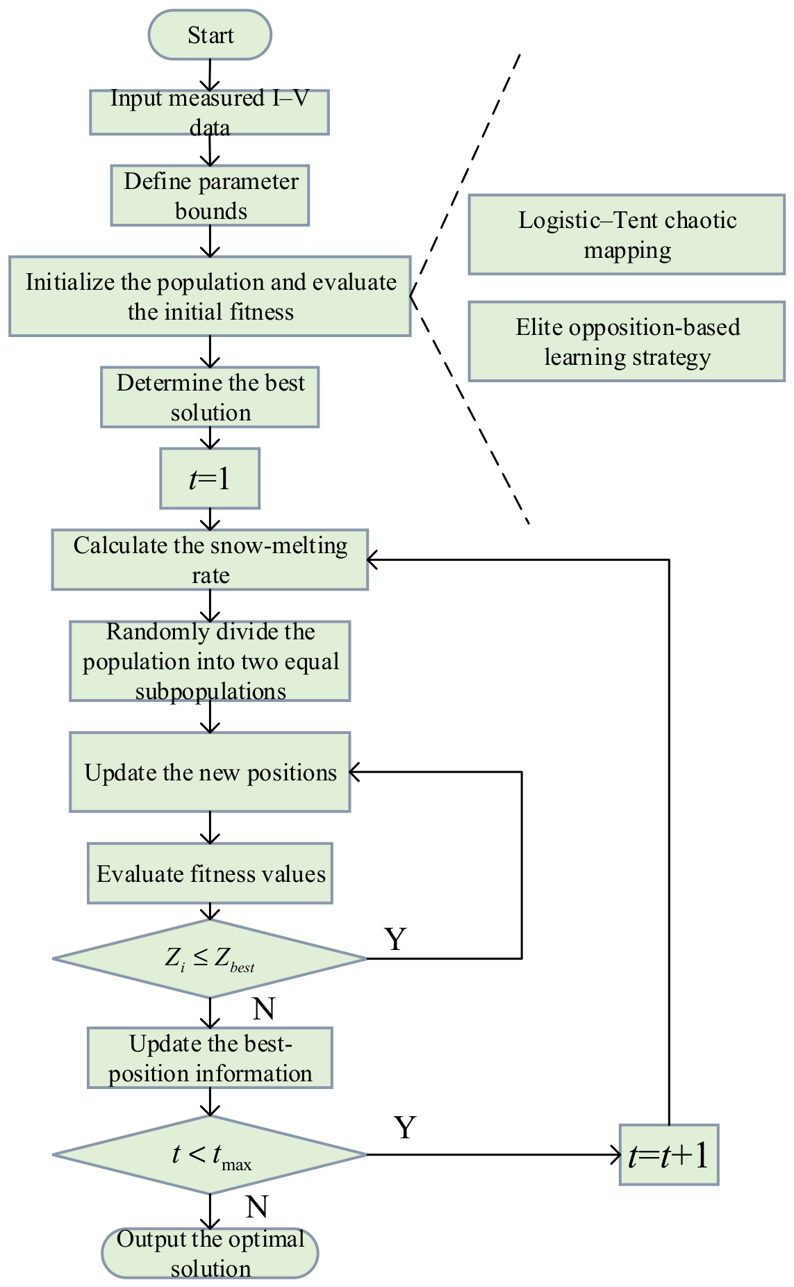
The overall LRSAO workflow incorporating chaotic initialization and elite opposition-based learning is shown in Figure 2.

3.2. RFDB and Lévy Flight Improvements

The fitness-distance balance (FDB) strategy guides metaheuristic search by jointly considering objective fitness and distance from the current best candidate [24]. For a population P and its fitness vector FV, the representation is

$$P\equiv \left[\begin{array}{ccc}{x}_{11}& \cdots & x_{1n}\\ ⋮& \ddots & ⋮\\ x_{m1}& \cdots & x_{mn}\end{array}\right], \mathrm{F}\mathrm{V}\equiv \left[\begin{array}{c}{f}_1\\ ⋮\\ f_m\end{array}\right]$$

(28)

where P is the candidate population matrix, FV is the fitness-value vector, m is the number of candidate solutions, and n is the number of design variables. The distance vector and FDB score are calculated as follows:

$$\forall P_i,\hspace{0.33em}{D}_{P_i}=\sqrt{{\left(x_{1\left[i\right]}-x_{1\left[\mathrm{b}\mathrm{e}\mathrm{s}\mathrm{t}\right]t}\right)}^2+\cdots +{\left(x_{n\left[i\right]}-x_{n\left[\mathrm{b}\mathrm{e}\mathrm{s}\mathrm{t}\right]t}\right)}^2}$$

(29)

$$Dp\equiv {\left[\begin{array}{c}{d}_1\\ ⋮\\ d_m\end{array}\right]}_{m\times 1}$$

(30)

$$\forall P_i,\hspace{0.33em}{S}_{P_i}=w\times {\mathrm{n}\mathrm{o}\mathrm{r}\mathrm{m}\mathrm{F}\mathrm{V}}_i+\left(1-w\right)\times {\mathrm{n}\mathrm{o}\mathrm{r}\mathrm{m}\mathrm{D}}_{P_i}$$

(31)

$$Sp\equiv {\left[\begin{array}{c}{S}_1\\ ⋮\\ S_m\end{array}\right]}_{m\times 1}$$

(32)

where X_best is the current best candidate solution, D_p is the distance vector, d_i is the distance between the i-th candidate solution and X_best, S_p is the FDB score vector, w is the weight coefficient, normFV is the normalized fitness vector, and normD_p is the normalized distance vector. To avoid repeatedly selecting only the highest-scoring candidate, roulette wheel selection (RWS) is introduced into the FDB mechanism [25], forming the RFDB mating-pool update

$$\left\{\begin{array}{l}{X}_{pbest}^G=X_{\mathrm{R}\mathrm{F}\mathrm{D}\mathrm{B}\left(rw\right)}^G\\ X_{pworst}^G=X_{\mathrm{R}\mathrm{F}\mathrm{D}\mathrm{B}\left(rw\right)}^G\\ X_r^G=X_{\mathrm{R}\mathrm{F}\mathrm{D}\mathrm{B}\left(rw\right)}^G\end{array}\right.$$

(33)

where the letter R in RFDB denotes the roulette wheel selection mechanism. The updated mating pool is generated according to roulette wheel probability rather than by always selecting only the highest-scoring candidate. Hybrid metaheuristic algorithms have also been developed for structural single-objective engineering optimization [26] and for constrained photovoltaic cell and module optimization [27]. Finally, Lévy flight (LF), which has also been combined with FDB in engineering optimization problems [28], is used as a perturbation mechanism. Its heavy-tailed step-length distribution preserves local fine search while allowing occasional long-distance jumps:

$$Lévy\left({\alpha }_{LF}\right)=s_{LF}\times {\displaystyle \frac{x}{{\left|y\right|}^{1/{\alpha }_{LF}}}}$$

(34)

where Lévy(α_LF) is the Lévy flight step length, α_LF is the stability index, x and y are random variables used to generate the Lévy step, and s_LF was set to 0.05 is the step-size scaling coefficient. The integrated RLFDB-LRSAO algorithm therefore consists of four teachable modules: chaotic initialization, elite opposition-based learning, RWS-enhanced FDB selection, and Lévy flight perturbation. These modules can be explained separately in class and then integrated into the complete PEMFC parameter identification workflow.

3.3. Rationale for Combining RFDB and Lévy Flight Perturbation

RFDB and Lévy flight perturbation are combined because they intervene at different stages of the search process. RFDB modifies candidate selection: it evaluates both solution quality and spatial distance from the current best solution, and roulette wheel sampling avoids deterministically selecting the same highest-scoring candidate at every update. Its purpose is to preserve useful diversity while retaining fitness guidance. Lévy flight modifies the displacement distribution after a candidate has been selected: frequent short steps support local refinement, whereas occasional long jumps provide a mechanism for leaving a locally concentrated region.

This division of roles is relevant to PEMFC parameter identification because the empirical parameters are strongly coupled and different parameter combinations may produce similar voltage curves. In such a landscape, candidate-selection diversity and non-Gaussian positional perturbation address complementary risks—premature selection around a narrow region and insufficient movement away from that region. The methodological contribution is therefore the stage-wise integration of selection guidance and movement perturbation rather than the claim that RFDB or Lévy flight is individually new. Their use is presented to students as a mechanism-based design choice that must be judged through convergence, repeated-run stability, and comparative results.

The individual strategies are established techniques; the methodological novelty claimed here is their stage-wise coordination within LRSAO and their conversion into separately inspectable teaching modules. In contrast to a simple strategy list, the framework links each component to a distinct failure mode: nonuniform initialization, overconcentrated candidate selection, local search stagnation, or insufficient diagnostic feedback. Their independent and joint numerical contributions are evaluated in the ablation study in Section 5.3.

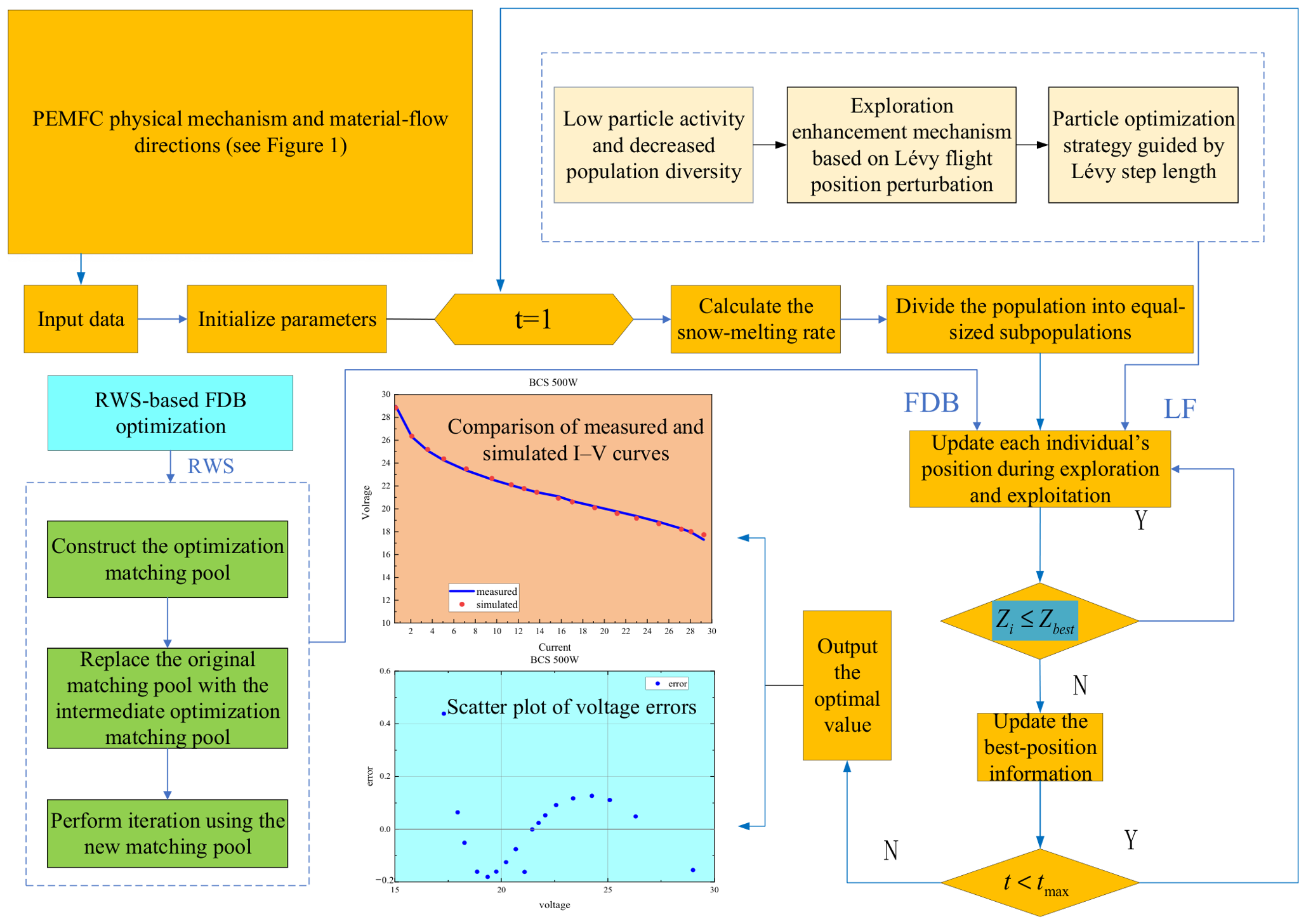
Figure 3 presents the overall flowchart of the RLFDB-LRSAO algorithm for PEMFC parameter identification, while the PEMFC physical mechanism is presented separately in Figure 1.

3.4. Computational Complexity

Let N denote the population size, D the number of decision variables, K the maximum number of iterations, and C_f the computational cost of one PEMFC objective function evaluation. For the baseline SAO, updating the population positions requires O(ND) operations per iteration, whereas fitness evaluation requires O(NC_f). The RFDB mechanism introduces distance calculation, normalization, score computation, and roulette wheel sampling, resulting in an additional complexity of O(ND+N). The Lévy flight perturbation further requires O(ND) operations. Therefore, the overall time complexity of RLFDB-LRSAO can be expressed as O[KN(C_f+D)], while its principal storage complexity is O(ND). In the PEMFC parameter identification problem, the objective function repeatedly evaluates the stack voltage over all measured current samples; therefore, objective function evaluation constitutes the dominant computational cost.

4. Virtual Simulation Teaching Design

4.1. Teaching Objectives and Experimental Process

The proposed experiment is suitable for courses in new-energy systems, electrical engineering, automation, intelligent optimization, engineering data analysis, and computational modeling. The teaching goal is not only to obtain a small fitting error but also to help students understand the full chain from electrochemical mechanism to mathematical model and from algorithmic search to performance evaluation. The experiment is arranged after students have learned basic circuit theory, energy conversion principles, numerical optimization, and introductory MATLAB programming.

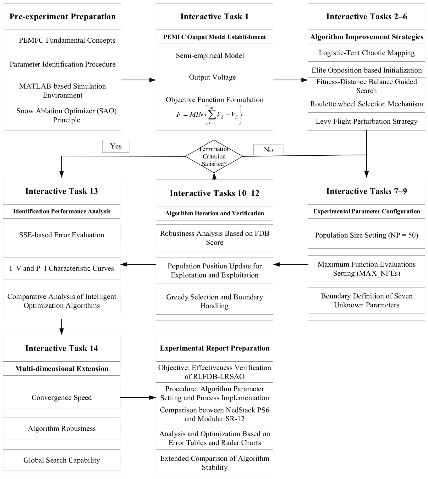
The complete student-facing teaching sequence is summarized in Figure 4.

The teaching process is organized into five stages. First, students complete pre-class preparation by reviewing PEMFC working principles, polarization losses, current-voltage characteristics, and parameter identification. Second, students construct the model by loading measured I–V data, setting the number of cells and operating conditions, and implementing the semi-empirical voltage equation. Third, students configure the algorithm by setting population size, maximum number of function evaluations (NFEs), search bounds, and random seed. Fourth, students visualize results by drawing convergence curves, I–V fitting curves, P–I curves, and error plots. Finally, students conduct reflection and optimization by explaining convergence behavior, adjusting parameter bounds, and comparing algorithm stability.

4.2. Software Environment and Code Scaffolding

The virtual experiment is implemented in MATLAB R2025a using standard matrix, random-number, numerical, file-input, and plotting functions; no external third-party software library is required. The source files are divided into data import, PEMFC voltage calculation, SSE evaluation, population initialization, candidate selection, position updating, boundary handling, and visualization modules. Fixed random seeds are controlled through the MATLAB rng function when reproducible comparisons are required. This organization allows intermediate quantities—including fitness values, selected candidates, convergence histories, and voltage residuals—to be inspected instead of treating the optimizer as a single black box executable.

For beginners, the instructor provides the measured data, the complete semi-empirical model, the baseline optimization routine, and plotting templates, while students configure bounds and algorithm parameters and interpret the results. Intermediate learners receive the model and program framework but complete the objective function, selected optimization modules, and comparative evaluation. Advanced learners can replace initialization, selection, or perturbation strategies, conduct robustness analyses, and extend the model. This code-scaffolding design makes the required student contribution explicit and reduces the likelihood that the learning activity becomes the passive execution of prepared software.

4.3. Process-Oriented Assessment and Classroom-Validation Design

The proposed process-oriented rubric contains four dimensions. Mechanism understanding accounts for 20% and is evaluated through pre-class questions and explanations of activation, ohmic, and concentration losses. Model correctness accounts for 25% and is evaluated by the implementation of the voltage equation, parameter bounds, and SSE objective. Algorithm implementation accounts for 25% and is evaluated through code completeness, reproducibility, module-level explanation, and convergence behavior. Result interpretation accounts for 30% and is evaluated through fitting curves, error analysis, repeated-run stability, discussion of parameter meaning, and recognition of model limitations. The rubric assesses both the computational product and the reasoning process, rather than assigning credit only for obtaining a small final error.

A small-scale qualitative teaching evaluation was conducted with 20 postgraduate students, focusing on task completion, programming practice, conceptual understanding, and reflective feedback. During the virtual experiment, students gained further experience in MATLAB programming, algorithm implementation, and computational analysis while their understanding of PEMFC parameter identification and intelligent optimization was strengthened. The modular experimental design also encouraged students to connect theoretical knowledge with research-oriented problem solving and to apply the acquired methods in subsequent scientific research activities. Some participants further extended the modeling and optimization methods to research projects involving invention patent applications and academic paper preparation and publication, providing additional evidence of the framework’s potential to support research and innovation training.

4.4. Hierarchical Learning Design

The experiment supports hierarchical learning. For beginners, the instructor may provide the complete model and ask students to modify only operating and algorithm parameters. Intermediate learners implement the objective function and selected optimization modules and compare baseline algorithms. Advanced learners can extend the experiment to multi-objective identification, constrained optimization, degradation-state modeling, or digital-twin-oriented online updating. Across levels, students are required to explain how a model assumption or algorithmic modification changes the numerical result. This design reflects a research–feeding–teaching pathway in which advanced optimization methods are reorganized into modeling, initialization, selection, perturbation, visualization, and evaluation tasks that learners can understand and reproduce.

5. Case Study and Result Discussion

5.1. Experimental Settings

Two representative commercial PEMFC stacks, NedStack PS6 and Modular SR-12, are selected as the main computational cases. The internal baselines LRSAO and FDB-LRSAO show the progressive effect of adding selection guidance before the complete RLFDB-LRSAO configuration. WOA represents a widely used encircling and spiral swarm search [29]; JS alternates ocean current and within-swarm movement [30]; MRFO uses chain, cyclone, and somersault foraging operators [31]; FDB-SDO represents a supply–demand optimizer enhanced by fitness-distance balance [32]; and RLFDB-COA provides a related example in which RFDB and Lévy flight are embedded in a different population framework. These algorithms were selected to cover distinct search mechanisms and to include both external metaheuristic baselines and internal progressive variants.

Table 1. Characteristics of the proton exchange membrane fuel cell (PEMFC) stacks.

Stack	Cells	Area (cm2)	Membrane (μm)	PH2 (bar)	PO2 (bar)	T (K)	JMAX (A/cm2)
NedStack PS6	65	240	178	1	1	343	1.4
Modular SR-12	48	62.5	25	1.47628	0.2095	323	0.672

,

Table 2. Search boundaries of PEMFC model parameters.

Parameter	NedStack LB	NedStack UB	SR-12 LB	SR-12 UB
δ1	−1.1997	−0.8532	−1.1997	−0.8532
δ2	0.001	0.005	0.001	0.005
δ3 (×10−5)	3.6	9.8	3.6	9.8
δ4 (×10−5)	−20	−10	−20	−10
λ	10	23	10	23
RC (×10−3 Ω)	0.1	0.8	0.1	0.8
b (×10−2 V)	1.36	50	1.36	50

and

Table 3. Parameter settings of comparison algorithms.

Algorithm	Parameter Setting
LRSAO	NP: 50, cSAO: 0.01
FDB-LRSAO	NP: 50, cSAO: 0.01
RLFDB-LRSAO	NP: 50, cSAO: 0.01
MRFO	NP: 50
RLFDB-COA	NP: 50, n-coy: 5, n-packs: 10
JS	NP: 50, β: 3, γ: 0.1
FDB-SDO	NP: 50
WOA	NP: 50, limit: 200, F: rand(0, 1)

Note: NP denotes population size; c_SAO denotes the SAO control coefficient used in the original computational settings. Algorithm-specific symbols retain the definitions given in their original references.

summarize stack characteristics, search boundaries, and algorithm settings. All algorithms use the same maximum number of function evaluations for the reported comparison.

5.2. Identification Accuracy and Stability

Table 4. Compact comparison of identification accuracy and stability.

Algorithm	NedStack SSE	NedStack Std	SR-12 SSE	SR-12 Std
LRSAO	1.2173813	4.12 × 10−2	6.13509800	3.00 × 10−5
FDB-LRSAO	1.2173710	2.20 × 10−2	6.13506572	1.04 × 10−5
RLFDB-LRSAO	1.2173340	1.93 × 10−2	6.13503904	2.48 × 10−6
MRFO	1.2242495	5.98 × 10−2	6.13638531	2.62 × 10−2
RLFDB-COA	1.2212930	1.09 × 10−2	6.13505690	1.80 × 10−4
JS	1.2604780	9.62 × 10−2	6.13773629	2.17 × 10−2
FDB-SDO	1.2180661	1.10 × 10−2	6.14173702	9.50 × 10−3
WOA	36.674284	1.12 × 101	56.21281114	7.10 × 100

reports the best SSE and repeated-run standard deviation available from the original computational study. RLFDB-LRSAO obtains best SSE values of 1.2173340 for NedStack PS6 and 6.13503904 for Modular SR-12. Its reported standard deviations are 0.0193 and 0.00000248, respectively. These values indicate favorable numerical accuracy and repeatability under the stated settings; however, the differences between several leading algorithms are small. The manuscript therefore does not interpret the best-value comparison alone as proof of statistical superiority. The nonparametric statistical evidence reported in Section 5.3 and Section 5.4 therefore pertains to the newly completed ablation benchmark experiments.

The above results are consistent with recent benchmark-oriented studies of PEMFC parameter identification and hybrid optimization algorithms [33], which emphasize joint evaluation in terms of solution accuracy, convergence speed, robustness, and engineering applicability.

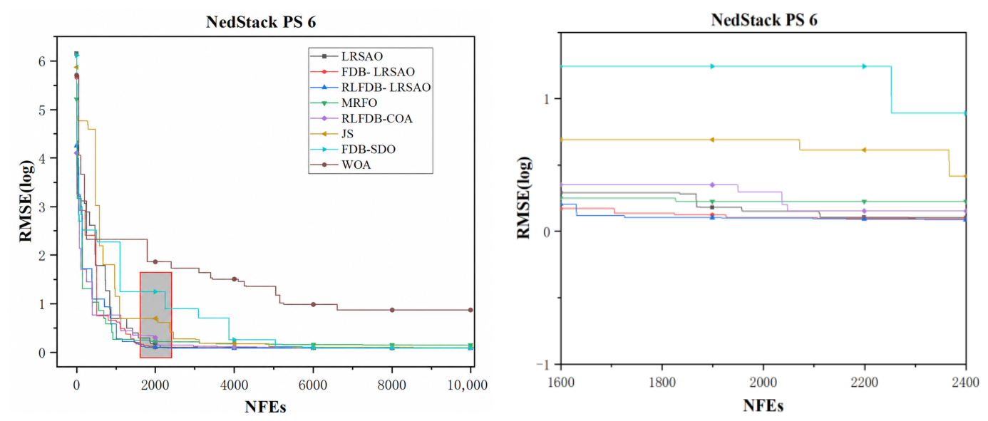
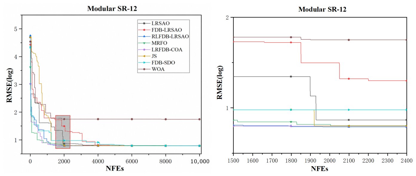
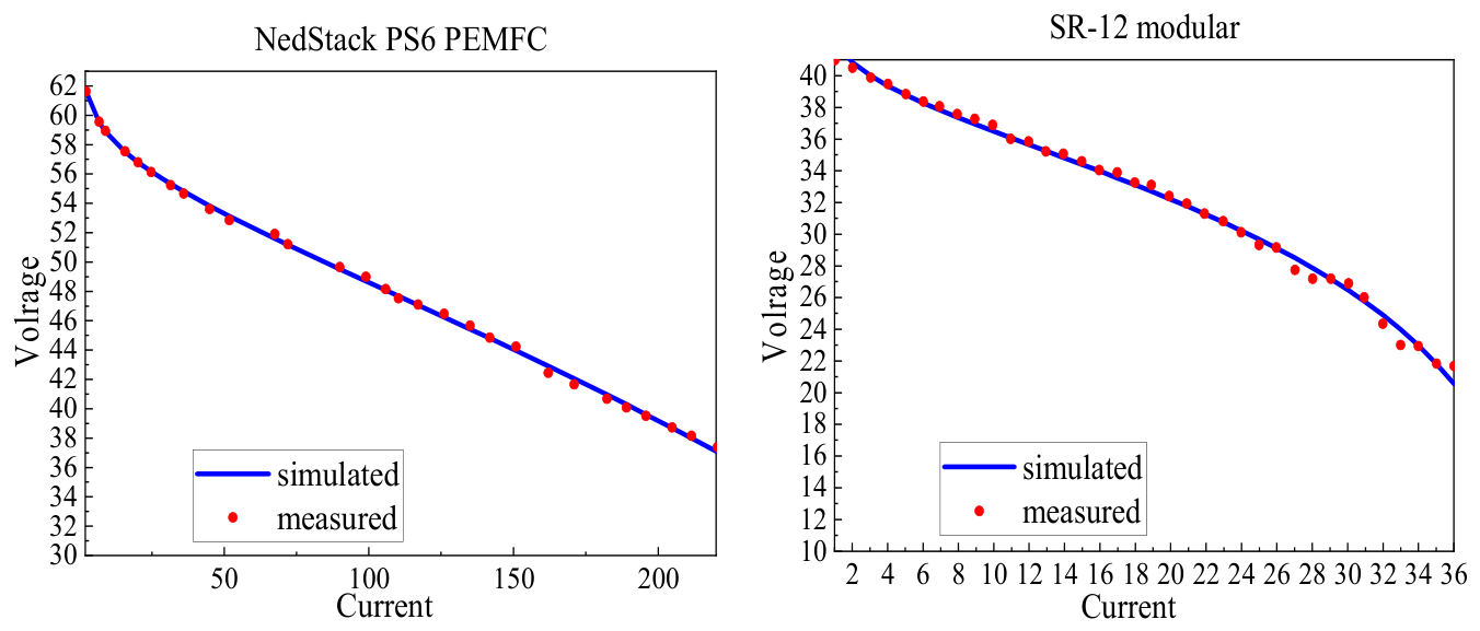
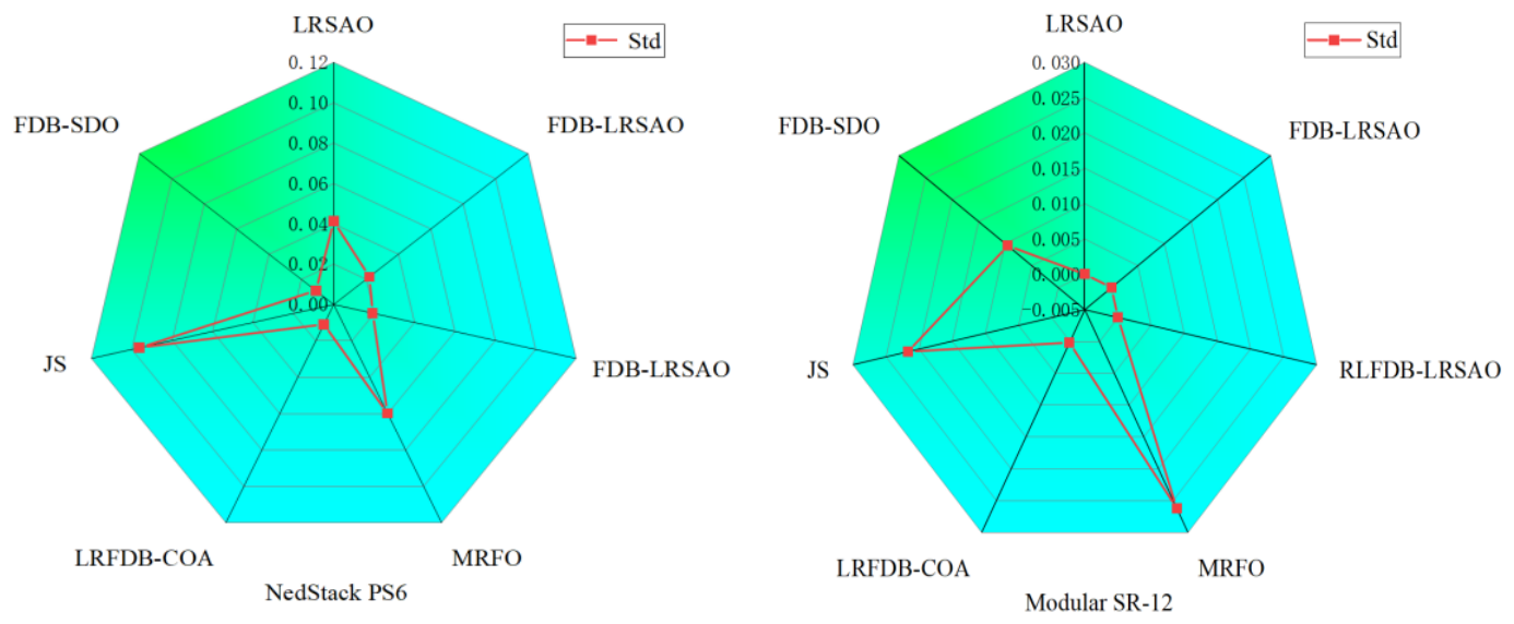
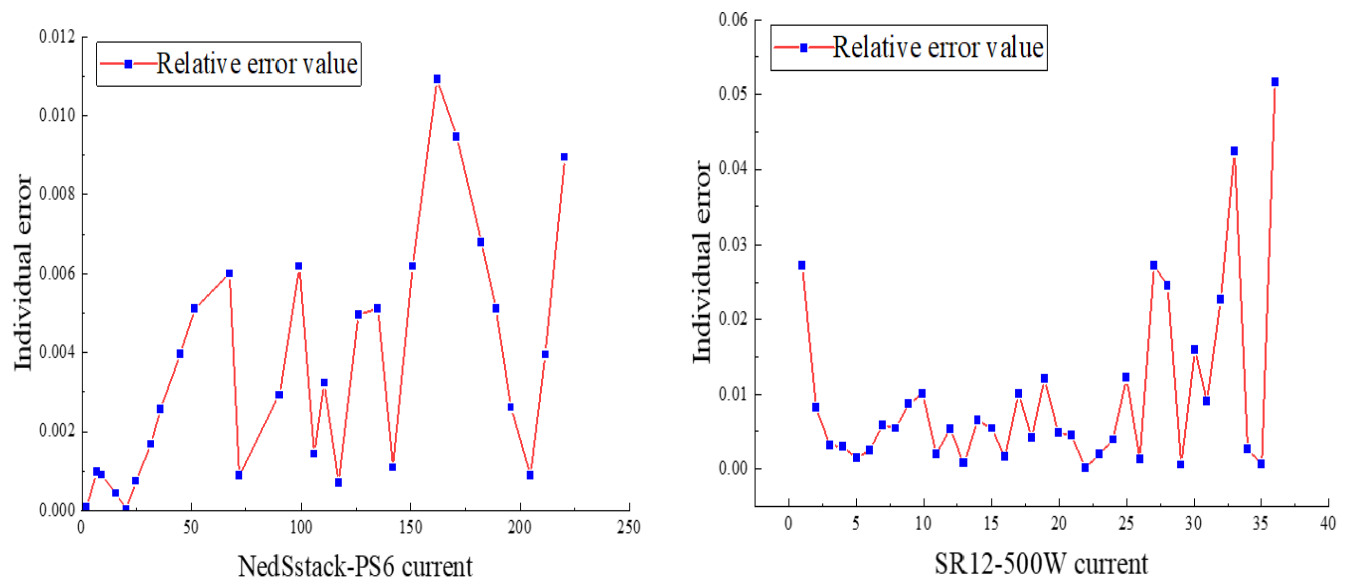
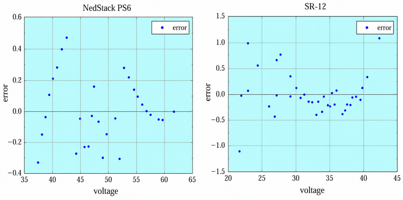
To further illustrate these performance characteristics, the representative convergence, fitting, stability, and error analysis curves are presented separately in Figure 5, Figure 6, Figure 7, Figure 8, Figure 9 and Figure 10. Figure 5 and Figure 6 show the convergence behavior and local magnification results for NedStack PS6 and Modular SR-12. Figure 7 compares the measured and simulated I–V curves for the two stacks, while Figure 8, Figure 9 and Figure 10 report the stability and error distributions of the identification results.

5.3. Ablation Study of Improvement Components

To isolate the contributions of the improvement components, seven configurations—SAO, LT-SAO, EOBL-SAO, LRSAO, RFDB-LRSAO, LF-LRSAO, and the complete RLFDB-LRSAO—were evaluated on six classical 30-dimensional benchmark functions: F1 (Sphere), F2 (Schwefel 2.22), F3 (Schwefel 1.2), F4 (Schwefel 2.21), F5 (Rastrigin), and F6 (Griewank). All configurations used a population size of 30, a fixed budget of 500 iterations, 30 independent paired runs, and identical paired random seeds. The exploration and exploitation subpopulations were maintained at equal size throughout the optimization process.

The Lévy-flight parameters were fixed before the final F1–F6 evaluation,

Table 5. Component-wise ablation results on six 30-dimensional benchmark functions.

Configuration	F1	F2	F3	F4	F5	F6
SAO	2.2417 × 10−25	4.0575 × 10−15	2.4924 × 10−13	2.2392 × 10−11	0	0
LT-SAO	7.2316 × 10−25	3.8963 × 10−15	3.3563 × 10−13	3.3748 × 10−11	0	0
EOBL-SAO	3.5812 × 10−26	3.7272 × 10−15	2.3538 × 10−13	2.0993 × 10−11	0	0
LRSAO	7.5061 × 10−26	8.5066 × 10−15	6.8167 × 10−14	5.3424 × 10−11	0	0
RFDB-LRSAO	2.9844 × 10−48	6.2202 × 10−26	2.0878 × 10−36	1.4459 × 10−22	0	0
LF-LRSAO	7.1958 × 10−26	4.3633 × 10−15	2.3852 × 10−13	3.4415 × 10−11	0	0
RLFDB-LRSAO	3.6753 × 10−48	5.8849 × 10−26	1.3072 × 10−35	2.4012 × 10−22	0	0

Note: Values are mean objective errors over 30 independent runs; lower is better. All experiments use D = 30, NP = 30, and 500 iterations. For F5 and F6, all configurations reached the theoretical optimum within double-precision numerical accuracy.

reports the mean objective errors and average ranks over 30 independent runs.

As shown in Table 5, RFDB-LRSAO achieved the best overall average rank of 2.17, followed by RLFDB-LRSAO with an average rank of 2.50. RFDB-LRSAO obtained the lowest mean errors on F1, F3, and F4, whereas RLFDB-LRSAO achieved the lowest mean error on F2. On F5 and F6, all seven configurations reached the theoretical optimum of zero within double-precision numerical accuracy; therefore, these two functions did not discriminate among the compared configurations.

Compared with LRSAO, RLFDB-LRSAO reduced the mean error from 7.506 × 10⁻²⁶ to 3.675 × 10⁻⁴⁸ on F1, from 8.507 × 10⁻¹⁵ to 5.885 × 10⁻²⁶ on F2, from 6.817 × 10⁻¹⁴ to 1.307 × 10⁻³⁵ on F3, and from 5.342 × 10⁻¹¹ to 2.40 × 10⁻²² on F4. These descriptive results indicate that RFDB provides the largest incremental accuracy gain beyond LRSAO on the tested continuous benchmark landscapes, while the additional contribution of Lévy flight is not uniformly beneficial.

5.4. Statistical Reliability of the Ablation Study

To further examine the statistical reliability of the ablation results, paired Wilcoxon signed-rank tests were conducted between RLFDB-LRSAO and the comparison algorithms based on 30 independent runs. The same six 30-dimensional benchmark functions reported in Table 5 were considered.

Table 6. Wilcoxon rank-sum test results of RLFDB-LRSAO against comparison algorithms.

Function	SAO	LT-SAO	EOBL-SAO	LRSAO	RFDB-LRSAO	LF-LRSAO
F1	3.01985935916215 × 10−11	5.4940524509652 × 10−11	1.46430688771503 × 10−10	3.01985935916215 × 10−11	3.68972585398101 × 10−11	3.01985935916215 × 10−11
F2	3.01985935916215 × 10−11	3.68972585398101 × 10−11	3.68972585398101 × 10−11	3.01985935916215 × 10−11	3.01985935916215 × 10−11	3.01985935916215 × 10−11
F3	3.01985935916215 × 10−11	4.97516644059341 × 10−11	5.4940524509652 × 10−11	3.01985935916215 × 10−11	1.47331749907827 × 10−7	3.01985935916215 × 10−11
F4	3.01985935916215 × 10−11	2.15439927669119 × 10−10	3.68972585398101 × 10−11	1.46430688771503 × 10−10	1.61322504446979 × 10−10	3.01985935916215 × 10−11

summarizes only the statistically significant comparisons between RLFDB-LRSAO and the main comparison algorithms.

As shown in Table 6, RLFDB-LRSAO achieves statistically significant improvements over most comparison algorithms on F1–F4, with p-values below 0.05 in most cases. However, the differences between RLFDB-LRSAO and RFDB-LRSAO are not statistically significant on several functions, indicating that RFDB provides the dominant contribution to optimization performance, while the additional Lévy flight perturbation offers problem-dependent benefits.

5.5. Preliminary Qualitative Teaching Evaluation

A small-scale qualitative teaching evaluation was conducted with 20 postgraduate students. Participant feedback indicated that visualization of polarization losses and voltage-fitting behavior, together with modular MATLAB implementation, was useful for strengthening programming practice and understanding the PEMFC parameter identification workflow. During the activity, students gained further experience in MATLAB programming, algorithm implementation, and computational analysis while their understanding of PEMFC parameter identification and intelligent optimization was strengthened. The modular design also encouraged students to connect theoretical knowledge with research-oriented problem-solving and to apply the acquired methods in subsequent scientific research activities. Some participants further extended the modeling and optimization methods to research projects involving invention patent applications and academic paper preparation and publication, indicating the potential of the proposed framework to support broader research and innovation training. Some participants still found the RFDB and Lévy flight mechanisms challenging. Because the evaluation was exploratory and did not include a control group, the findings are reported only as preliminary qualitative evidence rather than as a quantitative claim of learning improvement.

5.6. Discussion and Comparison with Related Studies

The proposed experiment differs from hardware-oriented or visualization-oriented virtual laboratories by requiring learners to formulate the semi-empirical model, implement the SSE objective, inspect optimization modules, and interpret repeated-run behavior. The recent 3D fuel cell teaching tool emphasizes system structure and performance-testing interaction, whereas the present framework emphasizes computational model identification and algorithm transparency. Conversely, recent PEMFC optimization studies provide extensive numerical benchmarking but are primarily research-oriented and do not specify student tasks, code scaffolding, or process-based assessment. The contribution of the present work lies in reorganizing this research workflow into a structured virtual experiment while clearly separating technical validation from evidence of learning effectiveness. The two main PEMFC cases support the technical feasibility of the proposed workflow.

5.7. Transferability and Limitations

The teaching workflow—from model construction to optimization and result interpretation—can be transferred to other electrochemical systems, but the physical model and identified parameters must be replaced.

The framework also has modeling and implementation limits. The present semi-empirical model is intended for specified steady-state temperature, pressure, and humidification conditions and does not explicitly represent transient gas transport, water management, degradation, or uncertainty. The two main commercial-stack datasets cannot represent all PEMFC power levels and operating regimes. A virtual experiment also cannot replace hands-on training in hydrogen safety, stack assembly, sensor operation, and fault handling. Future work should combine additional quantitative PEMFC cases, dynamic data, controlled classroom studies, and hybrid virtual–physical laboratory activities.

6. Conclusions

This study developed a MATLAB based virtual simulation framework for teaching-oriented PEMFC parameter identification. The framework integrates PEMFC mechanism analysis, semi-empirical model construction, SSE-based objective formulation, intelligent optimization, parameter configuration, visualization, and result interpretation. The proposed RLFDB-LRSAO combines Logistic–Tent chaotic initialization, elite opposition-based learning, RFDB, and Lévy flight. For the NedStack PS6 and Modular SR-12 cases, the best SSE values were 1.2173340 and 6.13503904, respectively, confirming the feasibility of the proposed parameter-identification workflow.

The benchmark experiments further evaluated the optimization performance. RLFDB-LRSAO showed statistically significant improvements over the non-RFDB configurations according to Wilcoxon tests. These results suggest that different improvement components contribute differently under the tested benchmark landscapes.

From an educational perspective, the preliminary qualitative evaluation with 20 postgraduate students indicated that the virtual experiment can support MATLAB programming practice, algorithm implementation, and understanding of PEMFC parameter identification and intelligent optimization. Future work will include additional PEMFC datasets, dynamic operating conditions, and larger controlled teaching studies to further validate the proposed framework.

References

1. Munciño, D.M.; Damian-Ramírez, E.A.; Cruz-Fernández, M.; Montoya-Santiyanes, L.A.; Rodríguez-Reséndiz, J. Metaheuristic and Heuristic Algorithms-Based Identification Parameters of a Direct Current Motor. Algorithms 2024, 17, 209. [Google Scholar] [CrossRef] [Scilit]
2. Radianti, J.; Majchrzak, T.A.; Fromm, J.; Wohlgenannt, I. A Systematic Review of Immersive Virtual Reality Applications for Higher Education: Design Elements, Lessons Learned, and Research Agenda. Comput. Educ. 2020, 147, 103778. [Google Scholar] [CrossRef] [Scilit]
3. Abd El-Mageed, A.A.; Al-Hamadi, A.; Bakheet, S.; Abd El-Rahiem, A.H. Hybrid Sparrow Search-Exponential Distribution Optimization with Differential Evolution for Parameter Prediction of Solar Photovoltaic Models. Algorithms 2024, 17, 26. [Google Scholar] [CrossRef] [Scilit]
4. Potkonjak, V.; Gardner, M.; Callaghan, V.; Mattila, P.; Guetl, C.; Petrović, V.M.; Jovanović, K. Virtual Laboratories for Education in Science, Technology, and Engineering: A Review. Comput. Educ. 2016, 95, 309–327. [Google Scholar] [CrossRef] [Scilit]
5. Kannan, S.K.; Diwekar, U. An Enhanced Particle Swarm Optimization Algorithm Employing Quasi-Random Numbers. Algorithms 2024, 17, 195. [Google Scholar] [CrossRef] [Scilit]
6. International Energy Agency. Global Hydrogen Review 2026; IEA: Paris, France, 2026; Available online: https://www.iea.org/reports/global-hydrogen-review-2026 (accessed on 10 August 2026).
7. Singla, M.K.; Ali, S.A.M.; Kumar, R.; Jangir, P.; Khishe, M.; Gulothungan, G.; Mahmoud, H.A. Revolutionizing Proton Exchange Membrane Fuel Cell Modeling through Hybrid Aquila Optimizer and Arithmetic Algorithm Optimization. Sci. Rep. 2025, 15, 5122. [Google Scholar] [CrossRef] [Scilit] [PubMed]
8. Zhang, M.; Amiri, A.; Xu, Y.; Bastin, L.; Clark, T. Self-Adaptive Digital Twin of Fuel Cell for Remaining Useful Lifetime Prediction. Int. J. Hydrogen Energy 2024, 89, 634–647. [Google Scholar] [CrossRef] [Scilit]
9. Jonassen, D.H.; Strobel, J.; Lee, C.B. Everyday Problem Solving in Engineering: Lessons for Engineering Educators. J. Eng. Educ. 2006, 95, 139–151. [Google Scholar] [CrossRef] [Scilit]
10. Yang, Y.; Li, H.B.; Wen, J.Y.; Yin, S.; Zhang, R. Reconstruction of New Engineering Practice Curriculum System in Electrical Engineering Discipline. Trans. China Electrotech. Soc. 2022, 37, 5074–5080. [Google Scholar] [CrossRef]
11. Li, J.; Liang, W. Effectiveness of Virtual Laboratory in Engineering Education: A Meta-Analysis. PLoS ONE 2024, 19, e0316269. [Google Scholar] [CrossRef] [Scilit] [PubMed]
12. Ma, L.; Xiong, J.; Wang, X.; Yan, Z.; Ji, L.; Zhang, J.; Xiao, H. Development of a Unity3D-Based Virtual Simulation Tool for Hydrogen Fuel Cell Performance Testing in Engineering Education. Comput. Appl. Eng. Educ. 2025, 33, e70095. [Google Scholar] [CrossRef] [Scilit]
13. Zawacki-Richter, O.; Marín, V.I.; Bond, M.; Gouverneur, F. Systematic Review of Research on Artificial Intelligence Applications in Higher Education—Where Are the Educators? Int. J. Educ. Technol. High. Educ. 2019, 16, 39. [Google Scholar] [CrossRef] [Scilit]
14. Kandidayeni, M.; Macias, A.; Amamou, A.A.; Boulon, L.; Kelouwani, S.; Chaoui, H. Overview and Benchmark Analysis of Fuel Cell Parameters Estimation for Energy Management Purposes. J. Power Sources 2018, 380, 92–104. [Google Scholar] [CrossRef] [Scilit]
15. Aldakheel, E.A.; Ismaeel, A.A.K.; El-Rifaie, A.M.; Khafaga, D.S.; Houssein, E.H.; Bouaouda, A.; Hashim, F.A.; Said, M. Extraction of PEM Fuel Cell Variables Based on Modified Hippopotamus Optimization Algorithm. Sci. Rep. 2025, 15, 33480. [Google Scholar] [CrossRef] [Scilit] [PubMed]
16. Zhou, L.; Shao, Y.; Zhou, H.; Yang, Y. An Improved SAO Used for Global Optimization and Economic Power Load Forecasting. Mathematics 2026, 14, 553. [Google Scholar] [CrossRef] [Scilit]
17. Liu, L.; Wang, J.; Zhang, C. A Personnel Emergency Evacuation Approach Considering Fire Risk Levels. Ocean Eng. 2026, 357, 125647. [Google Scholar] [CrossRef] [Scilit]
18. Kumari, S.; Singh, J.; Rawat, T.; Bansal, R.C. Multi-Objective Bi-Level Optimization for Planning and Operation of Electric Vehicle-Based Energy Storage Systems in Distribution Networks. J. Energy Storage 2026, 152, 120701. [Google Scholar] [CrossRef] [Scilit]
19. Tao, Z.; Zhang, C.; Xiong, J.; Hu, H.; Ji, J.; Peng, T.; Nazir, M.S. Evolutionary Gate Recurrent Unit Coupling Convolutional Neural Network and Improved Manta Ray Foraging Optimization Algorithm for Performance Degradation Prediction of PEMFC. Appl. Energy 2023, 336, 120821. [Google Scholar] [CrossRef] [Scilit]
20. Zhang, C.; Hu, H.; Ji, J.; Liu, K.; Xia, X.; Nazir, M.S.; Peng, T. An Evolutionary Stacked Generalization Model Based on Deep Learning and Improved Grasshopper Optimization Algorithm for Predicting the Remaining Useful Life of PEMFC. Appl. Energy 2023, 330, 120333. [Google Scholar] [CrossRef] [Scilit]
21. Ge, Y.; Zhang, C.; Liu, Q.; Zhang, X.; Chen, J.; Nazir, M.S.; Peng, T. A Novel Metaheuristic Optimizer Based on Improved Adaptive Guided Differential Evolution Algorithm for Parameter Identification of a PEMFC Model. Fuel 2025, 383, 133869. [Google Scholar] [CrossRef] [Scilit]
22. El-Fergany, A.A.; Hasanien, H.M.; Agwa, A.M. Semi-Empirical PEM Fuel Cells Model Using Whale Optimization Algorithm. Energy Convers. Manag. 2019, 201, 112197. [Google Scholar] [CrossRef] [Scilit]
23. Deng, L.; Liu, S. Snow Ablation Optimizer: A Novel Metaheuristic Technique for Numerical Optimization and Engineering Design. Expert Syst. Appl. 2023, 225, 120069. [Google Scholar] [CrossRef] [Scilit]
24. Kahraman, H.T.; Aras, S.; Gedikli, E. Fitness-Distance Balance: A New Selection Method for Meta-Heuristic Search Algorithms. Knowl.-Based Syst. 2020, 190, 105169. [Google Scholar] [CrossRef] [Scilit]
25. Asghari, K.; Masdari, M.; Gharehchopogh, F.S.; Saneifard, R. Multi-Swarm and Chaotic Whale-Particle Swarm Optimization Algorithm with a Selection Method Based on Roulette Wheel. Expert Syst. 2021, 38, e12779. [Google Scholar] [CrossRef] [Scilit]
26. Fakhouri, H.N.; Al-Shamayleh, A.S.; Ishtaiwi, A.; Makhadmeh, S.N.; Fakhouri, S.N.; Hamad, F. Hybrid Four Vector Intelligent Metaheuristic with Differential Evolution for Structural Single-Objective Engineering Optimization. Algorithms 2024, 17, 417. [Google Scholar] [CrossRef] [Scilit]
27. Liu, Q.; Zhang, C.; Li, Z.; Peng, T.; Zhang, Z.; Du, D.; Nazir, M.S. Multi-Strategy Adaptive Guidance Differential Evolution Algorithm Using Fitness-Distance Balance and Opposition-Based Learning for Constrained Global Optimization of Photovoltaic Cells and Modules. Appl. Energy 2024, 353, 122032. [Google Scholar] [CrossRef] [Scilit]
28. Duman, S.; Kahraman, H.T.; Guvenc, U.; Aras, S. Development of a Lévy Flight and FDB-Based Coyote Optimization Algorithm for Global Optimization and Real-World ACOPF Problems. Soft Comput. 2021, 25, 6577–6617. [Google Scholar] [CrossRef] [Scilit]
29. Mirjalili, S.; Lewis, A. The Whale Optimization Algorithm. Adv. Eng. Softw. 2016, 95, 51–67. [Google Scholar] [CrossRef] [Scilit]
30. Chou, J.S.; Truong, D.N. A Novel Metaheuristic Optimizer Inspired by Behavior of Jellyfish in Ocean. Appl. Math. Comput. 2021, 389, 125535. [Google Scholar] [CrossRef] [Scilit]
31. Zhao, W.; Zhang, Z.; Wang, L. Manta Ray Foraging Optimization: An Effective Bio-Inspired Optimizer for Engineering Applications. Eng. Appl. Artif. Intell. 2020, 87, 103300. [Google Scholar] [CrossRef] [Scilit]
32. Kati, M.; Kahraman, H.T. Improving Supply-Demand-Based Optimization Algorithm with FDB Method: A Comprehensive Research on Engineering Design Problems. J. Eng. Sci. Des. 2020, 8, 156–172. [Google Scholar] [CrossRef] [Scilit]
33. Hachana, O.; El-Fergany, A.A. Efficient PEM fuel cells parameters identification using hybrid artificial bee colony differential evolution optimizer. Energy 2022, 250, 123830. [Google Scholar] [CrossRef] [Scilit]
Figure 1. Basic operating mechanism of a proton exchange membrane fuel cell. Arrows indicate the directions of hydrogen and air supply, proton and electron transport, and water and heat removal.
Algorithms 19 00708 g001
Figure 2. Workflow of the Logistic–Tent reverse snow ablation optimizer (LRSAO) incorporating chaotic initialization and elite opposition-based learning.
Algorithms 19 00708 g002
Figure 3. Overall flowchart of the RLFDB-LRSAO algorithm for PEMFC parameter identification.
Algorithms 19 00708 g003
Figure 4. Overall workflow of the PEMFC parameter identification virtual simulation experiment. SAO, snow ablation optimizer; SSE, sum of squared errors; NP, population size; MAX_NFEs, maximum number of function evaluations.
Algorithms 19 00708 g004
Figure 5. Convergence curves and local magnification for NedStack PS6.
Algorithms 19 00708 g005
Figure 6. Convergence curves and local magnification for Modular SR-12.
Algorithms 19 00708 g006
Figure 7. Comparison between measured and simulated I–V curves of two PEMFC stacks.
Algorithms 19 00708 g007
Figure 8. Radar analysis of standard deviation values for PEMFC parameter identification.
Algorithms 19 00708 g008
Figure 9. Absolute relative errors of RLFDB-LRSAO for PEMFC parameter identification.
Algorithms 19 00708 g009
Figure 10. Absolute errors of RLFDB-LRSAO for two PEMFC parameter identification cases.
Algorithms 19 00708 g010