XAI-Guided Graph-Based Feature Engineering and Heterogeneous Ensemble Learning for Android Malware Detection

Abstract

Android malware continues to evolve in sophistication, creating a need for accurate, efficient, and interpretable detection mechanisms. This paper proposes a novel Android malware detection framework that integrates graph-based software engineering analysis, explainable artificial intelligence (XAI), and heterogeneous ensemble learning. The framework decompiles Android applications, constructs call graphs and control flow graphs, and extracts structural, functional, and behavioral software engineering metrics that are transformed into statistical feature representations. To improve feature quality and reduce dimensionality, LIME and SHAP are engineered into a threshold-based feature relevance mechanism, reducing the original 89 features to 65 and 61 features, respectively. A new heterogeneous ensemble classifier, RF–LNN–GRU, is then introduced to combine the complementary strengths of random forest, lightweight neural networks, and gated recurrent units through asymmetric probabilistic voting. Experiments conducted on 10,365 Android applications demonstrate that the proposed framework consistently outperforms conventional machine learning and ensemble baselines, achieving a detection rate of 98.98%, an F1-score of 96.2%, and an AUC of 98.1% while maintaining an inference latency below 0.4 ms per sample. These results demonstrate that the proposed combination of graph-derived software engineering metrics, XAI-guided feature engineering, and heterogeneous ensemble learning provides an effective and computationally efficient solution for Android malware detection.

1. Introduction and Motivation

The rapid evolution of cyber threats has created an increasingly complex challenge for securing software systems, particularly in the mobile ecosystem, where Android dominates the market share [1,2]. While traditional security measures rely heavily on human expertise, the sheer volume and sophistication of modern cyberattacks necessitate the development of intelligent automated defense mechanisms [3]. Cyberattackers employ various techniques to deploy and conceal malicious applications, including code obfuscation to disguise true functionality and the generation of clones or variants. Detecting such threats presents several challenges: (a) adapting to the rapidly evolving malware landscape, particularly the continuous emergence of new variants; (b) automating adaptation mechanisms; and (c) ensuring timely and effective responses to real-time threats. Adversaries continuously devise new techniques to evade detection, with obfuscation and variant generation emerging as particularly challenging threats to address [4].

Recent studies have highlighted the limitations of signature-based and traditional machine learning approaches in detecting sophisticated malware [5]. Although these methods can identify known patterns, they often struggle with new variants and obfuscated malicious code. This challenge is particularly acute in the Android ecosystem, where the open nature of the platform and the vast number of applications create abundant opportunities for malware distribution [6]. The Android platform’s flexibility, which allows developers to create a wide range of applications, also makes it a prime target for malicious actors. As a result, the need for robust, scalable, and intelligent malware detection systems has never been more critical. Prior research has explored various machine learning techniques in identifying and analyzing malware, including obfuscated and variant forms [7,8,9,10,11,12,13]. These approaches rely primarily on features such as permissions, API calls, visual representations, and predefined malicious functions. However, each method has its own set of limitations. For instance, models based on permissions and API calls require updates to accommodate newly introduced elements; visual pattern or image-based analysis is computationally expensive and not suitable for real-time detection; and reliance on known malicious functions can result in missing new malware variants. These shortcomings motivate the search for more fundamental structure-aware features.

Software engineering metrics offer a promising alternative. First used in the mid-1960s to measure productivity and programming effort, starting with lines of code [14], these metrics have since been applied to various software engineering activities, including bug and defect detection. Not all but some of these bugs and defects can lead to vulnerabilities [14]. Traditionally used for quality assurance and maintenance, software engineering metrics have shown promising potential in security applications [14]. Metrics such as fan-in, fan-out, and control flow graph parameters provide valuable insights into program structure and behavior. For example, fan-in and fan-out metrics can reveal the complexity of interactions between application components, while control flow graph metrics can identify unusual execution patterns that may indicate malicious behavior. Critically, because creating new malware is generally more challenging than modifying existing malware to produce a variant, these metrics are particularly useful for detecting clones and variants of original malware. Nevertheless, their application to Android malware detection remains largely unexplored, representing a significant research gap [15].

A second gap concerns interpretability. The emergence of explainable artificial intelligence (XAI) techniques, such as local interpretable model-agnostic explanations (LIME) and Shapley additive explanations (SHAP), has created new opportunities to enhance the transparency and effectiveness of machine learning-based security solutions [16]. These techniques address a critical limitation of traditional black-box approaches by offering transparency in feature selection and decision-making processes [17]. In malware detection, XAI can help security analysts to understand why a particular application is flagged as malicious, providing insights into the specific features or behaviors that triggered the detection. Such transparency is crucial for building trust in automated systems and enabling analysts to refine detection models over time. Very few works have used these techniques to optimize classification. One study by Alam et al. [18] used LIME and SHAP relevance values to improve file fragment classification, specifically improving multinomial classification. However, the integration of XAI techniques with software engineering metrics for Android malware detection remains largely unexplored in the existing literature.

Despite recent advances, two key gaps remain: the underexploited potential of software engineering metrics for malware detection and the lack of interpretability in feature selection. To address these gaps, we propose a novel framework that integrates software engineering metrics with explainable AI techniques. Our framework performs static Android malware analysis by examining Android application packages (APKs), from which structural and behavioral software engineering metrics are extracted. LIME and SHAP are then employed for feature analysis and reduction, followed by binary classification for malware identification. By combining structure-aware software engineering metrics with XAI-guided feature interpretation, the proposed framework aims to improve both detection robustness and interpretability in Android malware analysis.

Contribution

The main contributions of this paper are summarized as follows:

• We propose a unified graph-based Android malware detection framework that systematically integrates static program analysis, graph-derived software engineering metrics, XAI-guided feature engineering, and heterogeneous ensemble learning into a single end-to-end pipeline for malware classification.
• We introduce an XAI-guided feature engineering strategy in which LIME and SHAP are employed as feature relevance estimation techniques to identify and eliminate less informative graph-based software metrics prior to model training, thereby reducing the feature space while preserving classification performance.
• We develop RF–LNN–GRU, a heterogeneous ensemble classifier that combines the complementary strengths of random forest, lightweight neural networks (LNNs), and gated recurrent units (GRUs) through asymmetric thresholding and hybrid voting, enabling tree-based learning, nonlinear representation learning, and contextual feature interaction modeling within a unified decision framework.
• We conduct a comprehensive empirical evaluation, including comparisons with baseline models, component-wise ablation studies, and computational cost analysis, on a benchmark dataset of 10,365 Android applications collected from three independent malware repositories. The proposed framework achieves a detection rate of up to 98.98%, an F₁-score of 96.3%, and an AUC of 98.1% while maintaining low inference latency.

The proposed framework establishes a unified pipeline that integrates graph-derived software engineering metrics, XAI-guided feature engineering, and heterogeneous ensemble learning for Android malware detection. Although the individual components are established techniques, their integration into a cohesive end-to-end framework, together with the use of LIME and SHAP for feature relevance estimation rather than post hoc prediction explanation, provides an effective and interpretable solution for Android malware detection.

The remainder of this article is organized as follows. Section 2 reviews the related work, while Section 3 presents the background concepts. Section 4 details the proposed framework. The performance evaluation of the proposed framework is presented in Section 5. Section 6 concludes the article and outlines future research directions that could further enhance the capabilities of Android malware detection systems.

2. Related Work

The existing Android malware detection approaches can be broadly categorized into static analysis, dynamic analysis, and hybrid analysis techniques.

2.1. Static Analysis

Static analysis detects malware without executing applications, making it computationally efficient and scalable. Existing studies have employed diverse feature representations, including software metrics, permissions, API calls, opcodes, graph structures, and image-based transformations.

Several works have investigated software engineering metrics for malware detection. Tirkey et al. [19,20] and Blanc et al. [21] demonstrated the effectiveness of object-oriented and Android-specific code metrics for malware classification. Other studies explored software complexity metrics and resource-consumption characteristics as indicators of malicious behavior [22,23]. However, these approaches primarily focus on conventional software metrics and do not exploit structural and behavioral metrics derived from call graphs and control flow graphs (CFGs).

Permission-, API-, and opcode-based approaches have also been widely adopted [24,25,26,27,28]. While effective, these methods often depend on platform-specific artifacts that require updates as Android evolves. To capture richer structural information, graph-based techniques have been proposed, including API call graph analysis [29], CFG-based similarity analysis [30], and heterogeneous graph representations [7]. Deep learning approaches, including deep belief networks, neural decision forests, and image-based malware detection frameworks, have also shown promising results [8,31,32,33]. Nevertheless, many of these approaches incur substantial computational overhead or rely on predefined platform features.

Overall, static analysis remains attractive due to its efficiency, but the use of graph-derived software engineering metrics combined with explainable AI techniques remains largely unexplored.

2.2. Dynamic Analysis

Dynamic analysis observes application behavior during execution and is generally more resilient to obfuscation and packing techniques. Existing approaches have utilized runtime dependency graphs, register-level execution traces, behavioral features, network traffic characteristics, and system interactions to detect malicious activities [9,10,13,34,35,36,37,38].

Machine learning and deep learning models have been widely applied to dynamic features, often achieving high detection accuracy. Feature selection techniques have also been investigated to reduce dimensionality while maintaining effectiveness [11]. Despite these advantages, dynamic analysis typically requires sandboxing or emulation environments, incurs higher computational costs, and may fail to expose behaviors that are not triggered during execution.

2.3. Hybrid Analysis

Hybrid approaches combine static and dynamic features to leverage the strengths of both analysis paradigms. Previous studies demonstrated that integrating code-level and runtime information can improve malware detection performance compared with using either source independently [12,39]. For example, HGDetector [12] combines static function call graphs, network behavior graphs, and dynamic traffic features to construct comprehensive malware representations.

Although hybrid methods often achieve strong detection performance, they require multiple feature sources and increased computational resources. Moreover, existing hybrid frameworks primarily rely on permissions, API calls, network traffic, and behavioral indicators. To the best of our knowledge, the combination of graph-derived software engineering metrics with XAI-driven feature engineering using LIME and SHAP has not been systematically investigated for Android malware detection. This gap motivates the framework proposed in this paper.

Table 1 presents a comparative overview of the existing Android malware detection approaches and highlights research gaps that remain open for further investigation to advance this field.

Table 1. Comparative overview of recent Android malware detection methods.

Article	Method	Research Gaps
[38] (2026)	Self-attention to analyze dynamic behavioral APK sequences; incremental learning; TCN.	Datasets used for validation do not support pixnapping attacks; authors generated proxy attacks to overcome this limitation
[33] (2025)	Static analysis: YOLOv11; map APK to image of size of 256 × 256. XAI to explain the model.	Can be computationally intensive; may not be suitable for real-time deployment.
[11] (2025)	Hybrid analysis: Multi-wrapper feature selection (31 features) combining static/dynamic attributes.	Feature engineering complexity; scalability concerns.
[12] (2025)	Hybrid analysis: Combines static (function call graphs) and dynamic (network traffic) features with SVM.	Relies on known malicious functions; may miss unknown variants.
[9] (2025)	Dynamic analysis: Ensemble learning (bagging) with hybrid traffic/dynamic features.	High resource usage; limited to observable runtime behaviors.
[7] (2024)	Static analysis: Uses permission-related APIs and functionality graphs with MLP.	Requires updates for new Android versions due to API dependencies.
[10] (2024)	Dynamic analysis: Grayscale image transformation of traffic/behavioral features + deep learning.	May struggle with encrypted traffic or evasion techniques.
[13] (2024)	Knowledge search + model compression (distillation/NAS) for sustainability.	Requires frequent retraining for evolving threats.
[30] (2021)	Static analysis: Natural language processing and similarity index model of MAIL control flow patterns.	Computationally intensive; may not detect zero-day malware.
[8] (2021)	Static analysis: Bytecode-to-image conversion with temporal convolutional networks (TCNs).	Computationally intensive; limited to visual patterns.

3. Background

In this section, we explain some of the terms and concepts used in this paper. We also discuss and explain the different classifiers used in this paper.

3.1. Explainable Artificial Intelligence (XAI)

For a formal definition and a more detailed explanation of XAI, the readers are referred to [40]. Here, we briefly explain the main operations of an XAI system. XAI aims to improve the transparency of machine learning models by identifying the factors that influence their predictions. XAI techniques can be broadly categorized into inherently interpretable models, feature-based interpretation methods, and post hoc explanation techniques. In this work, we employ two model-agnostic XAI methods, LIME (local interpretable model-agnostic explanations) [41] and SHAP (Shapley additive explanations) [42], as feature relevance estimation techniques to identify the most informative software engineering metrics prior to classifier training.

3.2. LIME

LIME is an explainable AI technique that plays a key role in enhancing the understanding of the model and, hence, the decision-making process. LIME uses a local interpretable surrogate of the original model to enhance interpretability. This surrogate mimics the behavior of the original model, allowing it to identify which input features have the greatest impact on each prediction’s output. In this paper, we have used this property of LIME to select the most relevant features for our model.

LIME focuses on explaining predictions for individual instances rather than the entire model. It perturbs the input data around the instance of interest and observes changes in the model’s predictions. By analyzing these perturbations, LIME identifies which features are most influential for that particular prediction. LIME constructs a local surrogate model around an individual sample by perturbing its input features and observing the corresponding prediction changes. The resulting surrogate model estimates the contribution of each feature to the prediction within the local neighborhood of the sample.

In our proposed malware detection methodology, we utilize LIME to determine the importance of each software engineering metric for individual predictions. The local explanations generated by LIME help to identify which metrics are most influential in classifying an APK as malicious or benign. This selective emphasis aids in optimal feature selection by ensuring that only the most relevant metrics are retained for classification, improving model efficiency and accuracy. In the proposed framework, LIME is employed to estimate the relevance of graph-derived software engineering metrics. The resulting feature relevance scores are used to remove less informative features before classifier training, thereby reducing the feature space while preserving predictive performance.

3.3. SHAP

Similar to LIME, SHAP also plays a very important role in understanding machine learning models by utilizing the concept of Shapley values from game theory. Unlike LIME, which focuses on local approximations, SHAP provides a unified framework that offers both local and global interpretability. In SHAP, the contribution of a feature is computed by systematically considering all possible combinations of features and measuring the marginal impact of adding a specific feature to each subset. This process results in a Shapley value for each feature, representing its average contribution to the prediction across all such combinations.

Shapley values form the mathematical foundation of SHAP. The method provides a principled way to quantify each feature’s contribution to a machine learning model’s predictions. It works by systematically analyzing how much each feature influences the model’s output when introduced across every possible combination of other features. SHAP estimates feature importance using Shapley values from cooperative game theory, assigning each feature a contribution based on its average marginal effect across all feature combinations. Compared with LIME, SHAP provides both local and global estimates of feature relevance.

In our framework, SHAP complements LIME by offering a more mathematically grounded view of feature importance. By applying SHAP to the set of software engineering metrics extracted from APKs, we are able to quantify the individual impact of each metric on the model’s output. It also helps in identifying consistently influential features across different samples in the dataset.

In the proposed framework, SHAP complements LIME by providing an alternative estimate of feature relevance. The selected feature subsets are subsequently evaluated through the malware classification experiments.

3.4. Android Application Package (APK)

The proposed framework performs static malware analysis on Android application packages (APKs), the standard archive format used to distribute and install Android applications. Each APK contains application resources and a classes.dex file, which stores the compiled Java bytecode. For analysis, the APK is decompressed to extract the classes.dex file, which is converted into a JAR archive and subsequently decompiled to recover the Java source code. The recovered source code is then used to construct the function call graph and control flow graph from which the software engineering metrics employed by the proposed framework are extracted.

4. The Proposed Framework

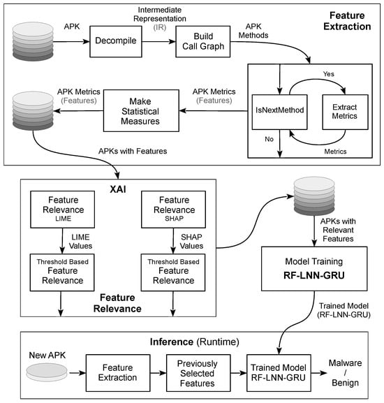
Android applications are packaged and distributed in the form of APKs (Android application packages). They are mostly written in Java programming language. We first decompile them into an intermediate language. Then we build a call graph of each APK and extract all the methods in this call graph. For each function in the APK, we build its control flow graph. Software engineering metrics are extracted for each function in the call graph. Next, we compute statistical measures of these metrics for each APK. These measurements form our set of features. We use XAI techniques like LIME and SHAP to identify the most relevant features from the existing set. These selected features are then used by a classifier to train and predict whether an APK is malware or benign. An overview of this proposed framework is shown in Figure 1. In the next sections, we describe in detail each of the components of this framework.

Figure 1. A high-level overview of the proposed framework.

The XAI feature relevance stage is executed only during model training to identify the most informative feature subset. These selected features are subsequently used to train the RF–LNN–GRU classifier. During malware detection, only the selected features are extracted and provided to the trained classifier; LIME and SHAP are not recomputed.

4.1. Decompilation

Decompilation is the process of converting an executable application to its source code or an intermediate language. Such decompilation makes it easier to perform certain analyses, such as call graph generation, on the application. There are different approaches to decompiling an APK. Some of them are: (1) Apktool is used to decompile an APK to smali files, and then the analysis is performed on the smali files; (2) Dex2jar is used to decompile an APK to Java .class files, and then the analysis is performed on the .class files. We adopted approach (2) because we want to analyze call graphs and CFG, and it is easier to perform such analysis on Java than on Smali files. We assume that the .class files are not encrypted.

Malware writers can use encryption or other obfuscation techniques to hide their malicious code. We perform static analysis without performing any decryption of the .class files. Therefore, we exclude from analysis the APK that contains encrypted .class files. Moreover, our technique performs structural and behavioral analysis of an APK that takes care of most of the other obfuscations.

The proposed framework first converts each APK into a JAR archive using the Dex2jar tool [43]. The resulting JAR contains the application’s Java bytecode extracted from the classes.dex file. We then employ an in-house analysis tool built on the SOOT framework [44], which translates the Java bytecode into its intermediate representation (Jimple) for static analysis. Using this representation, the tool constructs the application call graph and the control flow graph (CFG) of each function, from which the software engineering metrics used in the proposed framework are extracted, as described in Section 4.2.

4.2. Build Call Graph

An APK can have multiple execution paths. During runtime, any of these paths can be taken. To find a malicious application, it is necessary to build all these execution paths because any of these can be malicious. Before extracting all the methods in an APK, we build the call graph of an APK as follows.

Definition 1. 

A control flow graph depicts the flow of a software program as a directed graph and shows all the paths that can be traversed while running the program.

Definition 2. 

A call graph is a control flow graph where each node is a method and each edge is a call from a method to either itself or another method. Formally, it is a directed graph $CG=(M,E)$, where M is the set of methods and E is the set of call flow edges. A call flow edge from method $m_1$ to $m_2$ is denoted by $e=(m_1,m_2)$.

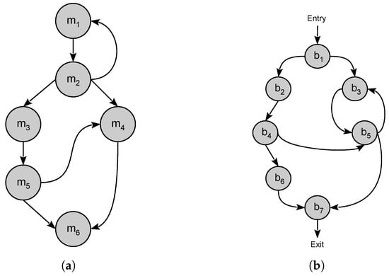
An example call graph is shown in Figure 2a. In this call graph, there are a total of six methods. There is one loop in this graph $m_1\Rightarrow m_2\Rightarrow m_1$. This call graph can be formally represented as

$$CG=(M,E)$$

where

$$M=\{m_1,m_2,m_3,m_4,m_5,m_6\}$$

and

$$\begin{array}{c}E=\{(m_1,m_2),(m_2,m_1),(m_2,m_3),(m_2,m_4),(m_3,m_5),\hfill \\ (m_4,m_6),(m_5,m_4),(m_5,m_6)\}\hfill \end{array}$$

Figure 2. Examples of a call graph and a CFG. (a) An example of a call graph. (b) An example of a CFG.

4.3. Software Engineering Metrics

After building the call graph, we extract software engineering metrics of each APK as follows.

We first extract all the methods from the call graph and then software engineering metrics from each of them as shown in Table 2. Before extracting these metrics, we also build the CFG [45] of each method as follows.

Table 2. Software engineering metrics extracted and employed in the proposed framework.

Family	Description
Method level
Fan-in	Number of methods calling this method
Fan-out	Number of methods called by this method
Parameters	Number of parameters passed to the method
Branches	Number of branches in the method
Invokes	Number of virtual, static, special, and interface invokes called in the method
Private	Is the method private?
Public	Is the method public?
Protected	Is the method protected?
Static	Is the method static?
CFG size	Number of nodes/blocks in the CFG of the method
LOC	Number of lines of code (statements) in all the blocks of the CFG of the method
APK level
NOM	Number of reachable methods in the APK

Definition 3. 

A basic block in a method is a sequence of statements that do not have any branches other than at the entry and exit points. A control flow edge represents the control flow between two basic blocks.

Definition 4. 

A CFG is a directed graph $G=(B,E)$, where B represents the set of basic blocks and E denotes the set of control flow edges. The control flow edge from the basic block $b_1$ to $b_2$ is denoted by $e=(b_1,b_2)$.

An example CFG is shown in Figure 2b. There are a total of seven nodes/blocks in this CFG. This CFG can be formally represented as

$$G=(B,E)$$

where

$$B=\{b_1,b_2,b_3,b_4,b_5,b_6,b_7\}$$

and

$$\begin{array}{c}E=\{(b_1,b_2),(b_1,b_3),(b_2,b_4),(b_3,b_5),(b_4,b_5),\hfill \\ (b_5,b_3),(b_4,b_6),(b_6,b_7),(b_7,b_5)\}\hfill \end{array}$$

4.4. Statistical Measurements

For all the method-level metrics of an APK listed in Table 2, we compute the following statistical measures: mean, median, range, minimum, maximum, standard deviation, variance, and sum. With one APK-level metric listed in Table 2 and eight measurements for the eleven method-level metrics, we get a total of 89 features. These 89 features are computed for each APK in the dataset. In this way, we build the set of features for all the APKs in the dataset.

We formally define a mathematical model of this set of features as follows:

Let $D=\{A_1,A_2,A_3,\dots ,A_k\}$, where k is the number of APKs in the dataset D. We assume that D is a labeled dataset; i.e., each APK in the dataset is labeled as either malware or benign. The set of features (statistical measurements) for an APK $A\in D$ is defined as $F=\{f_1,f_2,f_3,\dots ,f_{89}\}$. Now we define the set of all the features extracted and computed for all the APKs in the dataset D as

$$RF={\displaystyle \underset{a=1}{\overset{k}{⨆}}}\{F_a,c\}\left\{\begin{array}{cc}c=1\hfill & \mathrm{if}{A}_a\mathrm{is}\mathrm{malware}\hfill \\ c=0\hfill & \mathrm{otherwise}\hfill \end{array}\right.$$

(1)

We add a label c at the end of each set of features for an APK to use as the label for the class (malware/benign).

These sets of extracted features are then engineered using XAI [40] techniques, LIME, and SHAP, to select the most relevant and important features.

4.5. Feature Relevance—XAI

Feature selection is one of the major tasks in developing an efficient machine learning model. Extracting relevant features from a dataset requires special domain knowledge about the dataset. So far, we have extracted special features that represent the structural, functional, and behavioral properties of an APK. For extracting the relevant features, we employ and engineer two XAI techniques, LIME and SHAP. XAI is a branch of AI that is used to interpret and explain the methods used in AI. One method used for this purpose is to calculate the importance of input features in relation to an AI model’s output. In the framework proposed in this paper, we utilize LIME and SHAP, two popular model-agnostic techniques in XAI, to assess the relevance of input features to the model’s output.

4.5.1. LIME Relevance Values

LIME [40] builds an explainable proxy model of the original to explain each prediction of the original model. These proxies can be linear models or decision trees. The original model is explained by giving weights to the features in the original model.

We input the following parameters into the LIME explainer: features, training and testing data, and class names. We use ridge regression as the proxy model. We compute and collect the LIME relevance value $LV$ of a feature f for each APK and then the mean relevance LIME values $LVs$ of each feature f for all the classes (malware and benign) as follows:

$$LVs={\displaystyle \underset{f=1}{\overset{NF}{⨆}}}{\displaystyle {\displaystyle \underset{c=1}{\overset{NC}{⨆}}}}\left\{{\displaystyle \frac{{\sum }_{n=1}^{NS}R{V}_{f,n}}{NS}}\right\}$$

(2)

where $NF$ = total input features and $NC$ = total classes in the dataset. $NS$ = total APKs in class number c, and $R{V}_{f,n}$ is the relevance/importance value of the feature f in $nth$ APK.

4.5.2. SHAP Relevance Values

Similarly to LIME, SHAP [40] also builds and uses a simpler model that is the interpretable approximation of the original model. It provides the contribution of each feature to the prediction result by computing the Shapley value of each feature based on game theory.

We input the following parameters to the SHAP explainer: training and testing data. Random forest is used as the ensemble tree model. We compute and collect the relevance SHAP value $SV$ of the feature f for each APK and then the mean relevance SHAP values $SVs$ of each feature f for all the classes (malware and benign) as follows:

$$SVs={\displaystyle \underset{f=1}{\overset{NF}{⨆}}}{\displaystyle \underset{c=1}{\overset{NC}{⨆}}}\left\{{\displaystyle \frac{{\sum }_{n=1}^{NS}R{V}_{f,n}}{NS}}\right\}$$

(3)

where $NF$ = total input features and $NC$ = total classes in the dataset. $NS$ = total APKs in class number c, and $R{V}_{f,n}$ is the relevance/importance value of the feature f in $nth$ APK.

4.5.3. Threshold-Based Feature Relevance

After computing both the relevance LIME and SHAP values for all the features (in this paper, 89 features) in the dataset, we remove the irrelevant features. For this purpose, we conducted a threshold-based experiment. A threshold is computed and used to remove irrelevant features and keep the most relevant features. To enhance classification computing, we aim to reduce feature numbers by removing irrelevant features. For this purpose, separate thresholds for LIME and SHAP were calculated. Here is how we compute these thresholds.

We randomly selected a subset of the dataset to compute the LIME and SHAP relevance values using Equations (2) and (3). A higher value indicates a greater relevance to the input feature. The dataset was divided into 80% for training and 20% for testing. We conducted several classification experiments using different threshold values within the range $t_1$–$t_2$. The threshold that yielded the best results was selected. These steps were repeated for both LIME and SHAP to obtain two threshold values, denoted as $T_l$ for LIME and $T_s$ for SHAP. Using these threshold values, we removed the irrelevant features and got the respective final set of features, $FL$ of LIME and $FS$ of SHAP, as follows:

$$X_{FL}=\{v\mid v\in LVs\wedge v>T_l\}$$

(4)

and

$$X_{FS}=\{v\mid v\in SVs\wedge v>T_s\}$$

(5)

This relevant set of features is then used for training a classifier to classify Android applications (APKs) as malware or benign.

4.6. Classification (Detection)—Heterogeneous Ensemble Learning (RF–LNN–GRU)

Real-time detection of malware [46] is crucial to protect software systems. For this, a security software system needs to be operated, and threats need to be detected in real time. Smart devices with Android applications may not have enough resources to run a complex classification model. Moreover, our framework is, by design, restricted to two classes, benign and malware. These are our motivations not to use complex models for analyzing and detecting malware, and we choose a set of binary classifications to design our proposed framework.

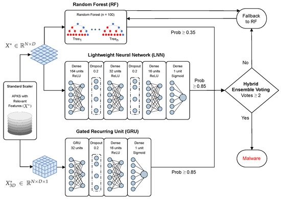
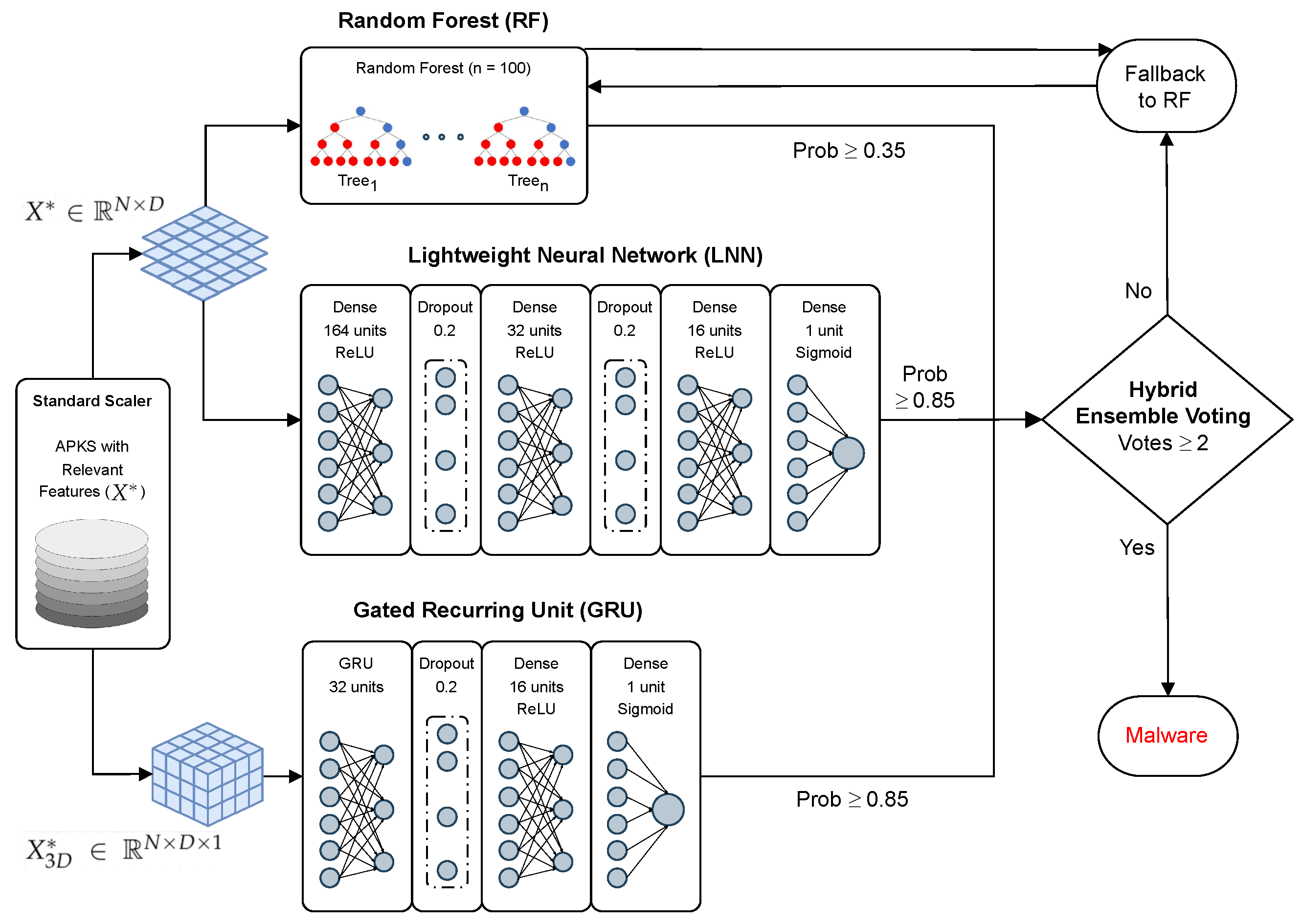
The proposed framework implements a heterogeneous ensemble learning system (RF–LNN–GRU, shown in Figure 3) optimized for malware detection using three distinct structural base classifiers: an RF, an LNN, and a GRU network. This complete pipeline consists of data standardization, parallel model optimization, asymmetrical probabilistic thresholding, and a hard-voting decision engine with a baseline fallback mechanism.

Figure 3. The proposed heterogeneous ensemble malware detection framework—RF–LNN–GRU.

4.6.1. Data Standardization and Spatial Transformation

To prevent operational data leakage, transformation parameters are computed exclusively from the training partition. Each raw feature matrix X is scaled to zero-mean and unit variance ($\mu =0,\sigma =1$):

$$X^{*}={\displaystyle \frac{X-\mu }{\sigma }}$$

(6)

The random forest and LNN models process this standardized two-dimensional representation $X^{*}\in {\mathbb{R}}^{N\times D}$, where N defines the number of samples and D denotes the feature dimensionality. Conversely, the gated recurrent unit (GRU) requires sequential dimensional ordering. The feature matrix is restructured into a three-dimensional tensor $X_{3D}^{*}\in {\mathbb{R}}^{N\times D\times 1}$ using array expansion, where each feature dimension is represented as an individual sequential element to enable the GRU to model dependencies among graph-derived software metrics. The imposed sequence reflects feature ordering rather than temporal evolution.

4.6.2. Random Forest (RF)

The RF model comprises an ensemble of $B=100$ independent bootstrap-aggregated decision trees. The final output probability for the target malware class ($y=1$) is derived by averaging the leaf node confidence outputs across all trees:

$$P_{RF}(y=1\mid x)={\displaystyle \frac{1}{B}}{\displaystyle \sum _{b=1}^B}{P}_b(y=1\mid x)$$

(7)

4.6.3. Lightweight Neural Network (LNN)

The LNN is a shallow multilayer perceptron consisting of three fully connected hidden layers interleaved with dropout regularization. The architectural dimensions scale sequentially as follows:

• Input Layer: D standardized features.
• Hidden Layer 1: 164 nodes with ReLU activation, followed by a 20% dropout layer.
• Hidden Layer 2: 32 nodes with ReLU activation, followed by a 20% dropout layer.
• Hidden Layer 3: 16 nodes with ReLU activation.
• Output Layer: 1 node with sigmoid activation.

The final layer uses a standard sigmoid activation function ($\sigma$) to compress the hidden representation vector into a continuous probability curve:

$$P_{LNN}(y=1\mid x)=\sigma \left(z\right)={\displaystyle \frac{1}{1+e^{-z}}}$$

(8)

The LNN is trained using the Adam optimizer (learning rate = 0.001) over a maximum of 100 epochs with a batch size of 64. To evaluate generalization capabilities and prevent overfitting, a 20% validation split is utilized during training, monitored by an early stopping callback with a patience of 5 epochs.

4.6.4. Gated Recurrent Unit (GRU) Network

The reshaped feature tensor $X_{3D}^{*}$ is processed by a GRU network to model dependencies among graph-derived software metrics. The network interprets feature vectors as temporal structural steps, flowing sequentially through the following layers:

• Input Layer: Sequential shape dimension of $(D,1)$.
• Recurrent Layer: GRU block with 32 units (returning only the final sequence state), followed by a 20% dropout layer.
• Hidden Layer: 16 nodes with ReLU activation.
• Output Layer: 1 node with sigmoid activation.

Internal reset and update gates track mathematical features sequentially to update the current state. The terminal output state is passed to the dense output block to produce the network’s final probability profile:

$$P_{GRU}(y=1\mid x)=\sigma \left(\mathrm{Dense}\left(\mathrm{GRU}\left(X_{3D}^{*}\right)\right)\right)$$

(9)

The GRU network uses the same Adam optimization settings and early stopping boundaries as the LNN, utilizing a 15% validation split to monitor convergence properties dynamically.

Although the extracted software metrics do not possess an inherent temporal ordering, representing the standardized feature vector as a one-dimensional sequence enables the GRU to model contextual dependencies among adjacent feature dimensions. In this work, the sequential formulation is not intended to capture temporal dynamics but rather to exploit the GRU’s gating mechanism for learning interactions and higher-order correlations between graph-derived software metrics. Similar sequence-based representations have been successfully adopted in prior studies employing recurrent neural networks for tabular and static feature classification, where the sequential processing serves as an effective architectural mechanism for modeling feature interdependencies rather than temporal evolution.

4.6.5. Asymmetric Probabilistic Thresholding

Each base classifier produces a probability estimate for the malware class. These probabilities are converted into binary decisions using classifier-specific thresholds, where a value of 1 denotes malware and 0 denotes benign. Different thresholds are assigned to the random forest and the neural networks to balance sensitivity and false positive rates.

$$V_{RF}=\left\{\begin{array}{cc}1,\hfill & P_{RF}\ge 0.35\hfill \\ 0,\hfill & \mathrm{otherwise}\hfill \end{array}\right.V_{LNN}=\left\{\begin{array}{cc}1,\hfill & P_{LNN}\ge 0.85\hfill \\ 0,\hfill & \mathrm{otherwise}\hfill \end{array}\right.V_{GRU}=\left\{\begin{array}{cc}1,\hfill & P_{GRU}\ge 0.85\hfill \\ 0,\hfill & \mathrm{otherwise}\hfill \end{array}\right.$$

(10)

4.6.6. Hybrid Ensemble Voting Logic with Fallback Control

The final prediction is obtained through a two-stage decision process. First, the binary decisions of the three base classifiers are aggregated by majority voting. If at least two classifiers predict malware, the sample is classified as malware. Otherwise, the random forest prediction is used as a fallback decision because of its stable baseline performance.

$$S_V=V_{RF}+V_{LNN}+V_{GRU}$$

(11)

A majority agreement constraint ($\ge 2$) is required to confirm malware. If the models completely disagree and fail to form an absolute voting consensus ($S_V<2$), a safe fallback loop activates. This process routes final decision responsibility directly back to the robust random forest baseline prediction:

$$\widehat{y}=\left\{\begin{array}{cc}1,\hfill & \mathrm{if}{S}_V\ge 2\hfill \\ V_{RF},\hfill & \mathrm{if}{S}_V<2\hfill \end{array}\right.$$

(12)

For probability-based evaluation metrics, such as ROC and AUC, a meta-probability score is computed as a weighted combination of the three classifier outputs:

$$P_{meta}=0.30·P_{RF}+0.35·P_{LNN}+0.35·P_{GRU}$$

(13)

5. Experimental Evaluation

We describe here the experimental study carried out to validate and evaluate the performance of the proposed framework. For this purpose, a different set of experiments were carried out. We also carried out experiments to compute the threshold used in the framework. We describe in this section the dataset used in the experiments, LIME and SHAP relevance value computation, computation of the threshold, experiments to validate the proposed framework, the obtained results, and a comparison with other such works. All the experiments were carried out on an Intel Core i-7 @ 2.8 GHz PC running Ubuntu with 16 GB of RAM.

5.1. Dataset

For an efficient and unbiased evaluation of our proposed framework, we selected, utilized, and built our dataset from three sets of real-world Android malware data. One of the sets is collected from the two different resources [47,48]. This set consists of a variety of samples from different families of malware. Most of these malware samples are piggybacked applications, such as ADRD, all the DroidKungFu families, DroidDream, DroidDreamLight, Geinimi, JSMSHider, and Pjapps. Others, like GoldDream and YZHC, are standalone malware applications. The other two sets, CICAndMal2017 [49] and CICMalDroid2020 [50], are collected from the Canadian Institute for Cybersecurity datasets. CICAndMal2017 contains malware samples from the following different categories: Adware, Ransomware, Scareware, and SMSMalware. All these categories consist of malware from 42 different families. For example, Adware and Ransomware have 10 unique families each, and Scareware and SMSMalware have 11 unique families each. CICMalDroid2020 contains malware samples from the categories Adware and SMSMalware. For these two sets, a detailed description can be found at [51]. The sample sizes range from $\sim$14 KB to $\sim$52 MB. The malware dataset consists of samples from a variety of families with different sizes.

The benign dataset consists of Android system programs, shared libraries, real-world Android applications collected from Google Play, and benign applications collected from CICAndMal2017 [49] and CICMalDroid2020 [50].

The distribution of the main dataset containing 10,365 samples, including malware and benign, as explained above, is shown in Table 3.

Table 3. Distribution of the main dataset consisting of 10,365 samples.

Family	Number of Samples
First Set
ADRD	20
AnserverBot	185
BaseBridge	122
DroidDream	16
DroidDreamLight	46
DroidKungFu1	30
DroidKungFu2	30
DroidKungFu3	254
DroidKungFu4	96
Geinimi	69
jSMSHider	12
KMin	50
Pjapps	56
YZHC	22
BENIGN	1002
TOTAL	2010
CICAndMal2017
Adware	102
Ransomware	101
SMSmalware	99
Scareware	107
BENIGN	474
TOTAL	883
CICMalDroid2020
Adware	1497
SMSmalware	4782
BENIGN	1193
TOTAL	7472
GRAND TOTAL	10,365

Partitioning of the dataset for different experiments, including LIME and SHAP relevance computation, threshold computation, and validation, is shown in Table 4.

Table 4. Partitioning of the main dataset of 10,365 samples for different experiments. The 2073 samples are randomly selected from the main training set of 8292 samples and not the main testing set of 2073 samples.

Experiment	Number of Samples	Samples Used for Training	Samples Used for Testing
LIME and SHAP relevance computation	2073	1658	415
Threshold computation	2073	1658	415
80/20 random hold-out validation (10 runs)	10,365	8292	2073

All the malware samples originate from three independent repositories and include numerous malware families, categories, derived variants, and obfuscated applications. Consequently, the evaluation encompasses substantial diversity in malware characteristics, providing a challenging benchmark for assessing the robustness of the proposed framework within the Android malware domain.

5.2. Evaluation Metrics

The framework proposed in this paper performs a binary classification; i.e., it predicts whether a new APK is either malware or benign. The most widely used matrix for evaluating and visualizing the performance of a binary classifier is the confusion matrix [52] and is represented as a table. It compares the predicted and actual values. Table 5 shows an example confusion matrix. We utilize this matrix to compute the following evaluation metrics.

Table 5. Confusion matrix for visualizing the performance of a binary (malware/benign) classifier.

	Malware	Benign
Malware	TP	FN
Benign	FP	TN

The basic components of this matrix are: TP, the true positive, is the number of correctly predicted malware samples (actually malware ⇒ predicted malware). FP, the false positive, is the number of incorrectly predicted benign samples (actually benign ⇒ predicted malware). TN, the true negative, is the number of correctly predicted benign samples (actually benign ⇒ predicted benign). FN, the false negative, is the number of incorrectly predicted malware samples (actually malware ⇒ predicted benign).

Precision is the number of samples (either malware or benign) predicted as malware that were actually malware and is defined as:

$$Precision={\displaystyle \frac{TP}{TP+FP}}$$

Detection rate (DR) is the number of actual malware samples correctly predicted as malware, also called recall or true positive rate, and is defined as:

$$DR={\displaystyle \frac{TP}{TP+FN}}$$

$F_1$-score is the weighted average of precision and recall and is defined as:

$$F_1-score={\displaystyle \frac{2TP}{2TP+FP+FN}}$$

Accuracy is the number of all the samples predicted correctly and is defined as:

$$Accuracy={\displaystyle \frac{TP+TN}{TP+TN+FP+FN}}$$

Receiver operating characteristic (ROC) [52] is a graphical plot that illustrates the diagnostic ability of a binary classifier as its discrimination threshold is varied. The curve plots the true positive rate (TPR) against the false positive rate (FPR) at various threshold settings. The nearer the curve is to the top-left corner, the more effective the model is.

Area under the curve (AUC) [52] quantifies the overall ability of the classifier to distinguish between classes, with a higher AUC (closer to 1) indicating better performance, while an AUC of 0.5 suggests that the classifier performs no better than random guessing. Generally, a higher AUC value signifies a better-performing model. The AUC metric is used in this paper as a single number to summarize the ROC curve.

The main purpose of this research is to prioritize malware prediction. Moreover, out of the three datasets used in this paper, one of them, CICMalDroid2020, has a larger number of malware than benign (Table 3).

ROC is ideal when ranking predictions, in our case, malware first, and is useful for evaluating models when classes are imbalanced. Therefore, we employed ROC curve and AUC to evaluate the performance of our proposed model.

5.3. LIME and SHAP Relevance Computation

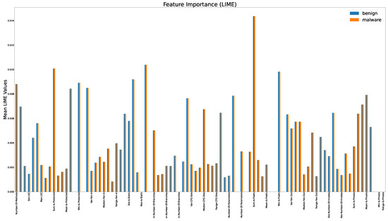
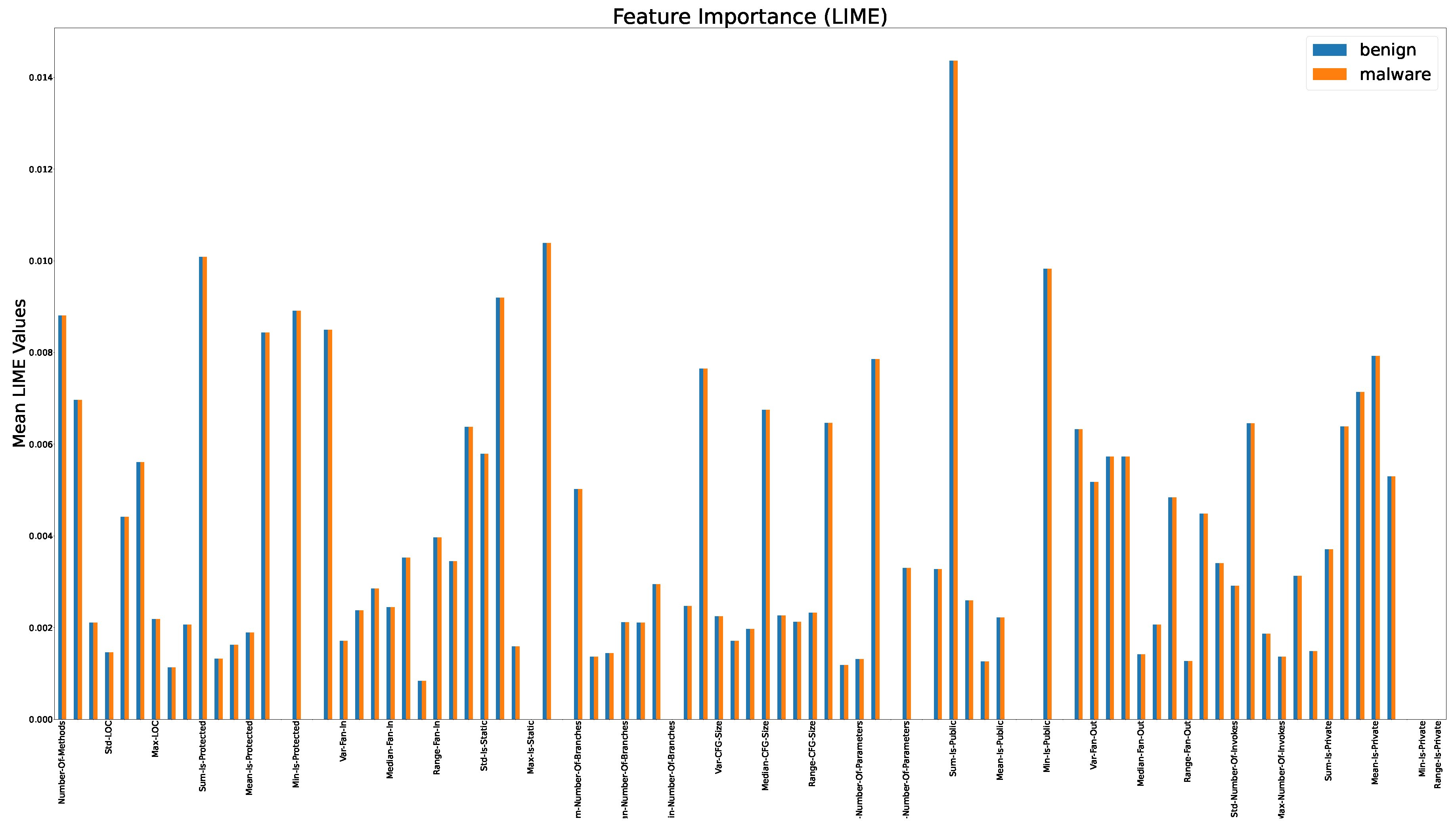
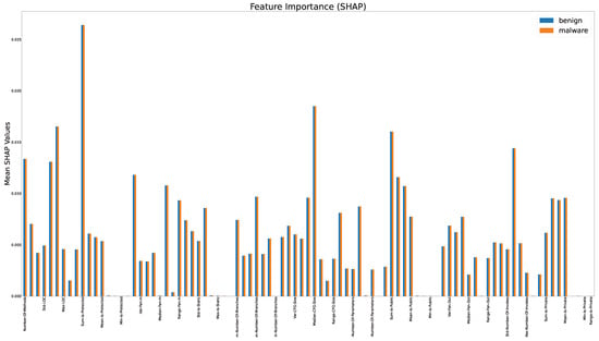
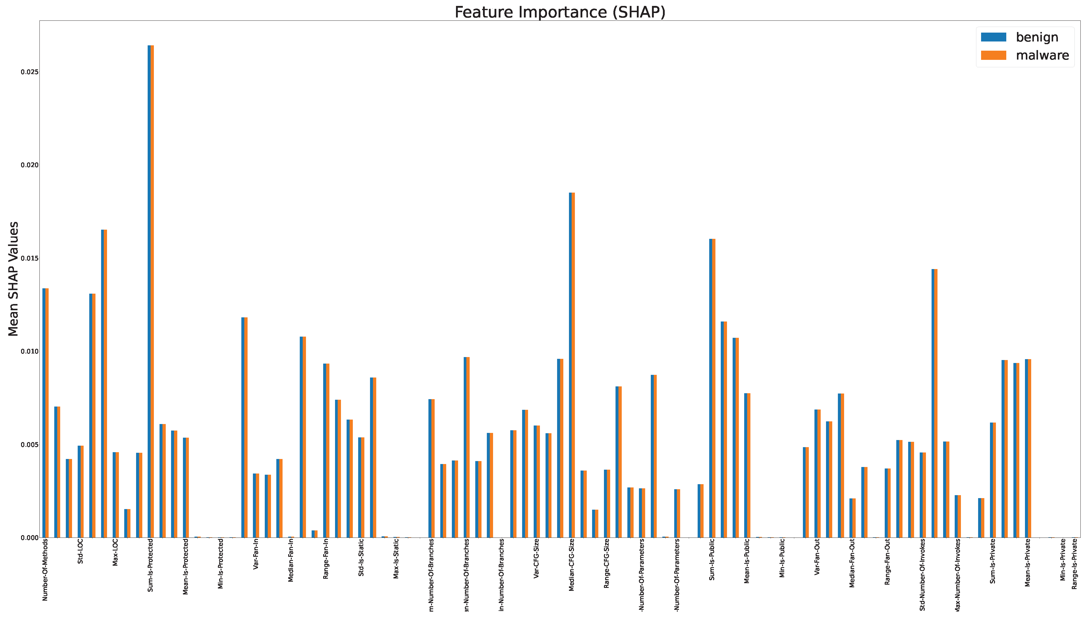
We first randomly chose a set of 2073 (20%) samples, 1573 malware and 500 benign, from the main training dataset of 8292 samples. This subset is then used to compute the relevance LIME and SHAP values, as discussed in Section 4.5.1 and Section 4.5.2 and listed in Equations (2) and (3). These relevance values of LIME and SHAP are shown in Figure 4 and Figure 5, respectively.

Figure 4. LIME relevance values. The X-axis displays the name of the feature. Because of the space constraints, only the fourth feature name is displayed. For example, feature number 1 → Number-Of-Methods is the metric NOM, i.e., the number of reachable methods, feature number 4 → Std-LOC is the standard deviation of the metric LOC in the APK, and so on.

Figure 5. SHAP relevance values. The X-axis displays the name of the feature. Because of the space constraints, only the fourth feature name is displayed. For example, feature number 1 → Number-Of-Methods is the metric NOM, i.e., the number of reachable methods, feature number 4 → Std-LOC is the standard deviation of the metric LOC in the APK, and so on.

As we can see in Figure 4 and Figure 5, these relevance values range from 0–0.0145 for LIME and from 0–0.0264 for SHAP. The LIME and SHAP relevance values at 75% are >0.0014 and >0.0003, respectively. Therefore, we need to compute different thresholds for each of them.

5.4. Threshold Computation

As mentioned before, a threshold is computed to remove the irrelevant features. A feature is removed if its relevance value is < the threshold, and we are left with the most relevant features. Here, we describe in detail the steps and experiments needed to compute this relevance threshold.

To determine suitable relevance thresholds, the threshold selection process was performed using a subset of 2073 samples extracted from the training data. For each candidate threshold, a different random 80/20 train–test split of this subset was used to compute the corresponding LIME and SHAP relevance values. Most, i.e., >75%, of the LIME and SHAP relevance values range from 0.0014 to 0.0003; therefore, candidate thresholds in the range of 0.005–0.0005 were evaluated, and the resulting classification performance was compared. The selected thresholds, $T_l$ = 0.0015 for LIME and $T_s$ = 0.0025 for SHAP, consistently provided the best trade-off between eliminating irrelevant features and preserving classification performance across the evaluated random splits. These thresholds were subsequently fixed and used throughout all the experiments on the complete dataset.

In Figure 4 there are 24 features with values < 0.0015. Feature numbers 4, 8, 11, 35, 51, 52, 60, 70, 73, 79, and 81 have values $<T_l$ = 0.0015; and feature numbers 15, 17, 31, 33, 40, 54, 56, 62, 63, 65, 87, 88, and 89 have zero values. Using LIME, we were able to remove 24 features. Similarly, in Figure 5, there are 28 features with values < 0.0025. Feature numbers 8, 14, 15, 16, 17, 22, 24, 30, 31, 32, 33, 48, 54, 62, 63, 64, 65, 70, 72, 79, 80, 81, 86, 87, and 89 have values $<T_s$ = 0.0025; and feature numbers 40, 56, and 88 have zero values. Using SHAP, we were able to remove 28 features.

Now we have two sets of the most relevant features, one of LIME and the other of SHAP. To validate and evaluate the performance of our proposed framework, two experiments were carried out using the main dataset of 10,365 samples, one with the LIME and the other with the SHAP most relevant sets of features.

In the proposed framework, LIME and SHAP are employed exclusively for feature relevance estimation and feature selection rather than for post hoc interpretation of individual classification decisions. Therefore, the evaluation focuses on the quality of the selected feature subsets and their impact on classification performance.

5.5. Performance Evaluation and Results

We conducted two sets of experiments, first with the baseline models and second with the proposed model. We also carried out ablation experiments. For the baseline models, we choose traditional machine learning algorithms, logistic regression, naive Bayes, and random forest. These baseline models were selected for the following reasons. First, they are well-established interpretable algorithms that require minimal hyperparameter tuning, making them suitable benchmarks for evaluating the relative performance improvement of our proposed heterogeneous ensemble (RF–LNN–GRU). Second, as discussed in Section 2, prior Android malware detection studies have frequently employed classifiers such as naive Bayes, random forest, and logistic regression-based feature selection; using these as baselines ensures comparability with existing work. Third, all three models are computationally lightweight, which aligns with our design goal of real-time detection, serving as lower-bound references for evaluating the trade-off between detection accuracy and inference latency. Finally, logistic regression (linear), naive Bayes (probabilistic), and random forest (ensemble of decision trees) represent distinct modeling paradigms that allow us to assess whether the proposed ensemble offers consistent improvements across different baseline characteristics. To facilitate the reproducibility of the proposed framework, the hyperparameter settings of the three constituent classifiers are summarized in Table 6. These parameters were selected empirically and used consistently throughout all the experiments.

Table 6. Hyperparameter configuration of the proposed RF–LNN–GRU framework.

Component	Hyperparameter	Value
Random forest	Number of trees ($n\_estimators$)	100
	Random seed	42
	Parallel processing ($n\_jobs$)	$-1$ (all CPU cores)
LNN	Architecture	164–32–16–1
	Hidden activation	ReLU
	Output activation	Sigmoid
	Dropout rate	0.2 (after first two hidden layers)
	Optimizer	Adam
	Learning rate	0.001
	Loss function	Binary cross-entropy
	Batch size	64
	Maximum epochs	100
	Validation split	20%
	Early stopping	Monitor = val_accuracy, patience = 5
GRU	Input shape	(Number of selected features, 1)
	GRU units	32
	Return sequences	False
	Dense layer	16 (ReLU)
	Output activation	Sigmoid
	Dropout rate	0.2
	Optimizer	Adam
	Learning rate	0.001
	Loss function	Binary cross-entropy
	Batch size	64
	Maximum epochs	100
	Validation split	15%
	Early stopping	Monitor = val_accuracy, patience = 5

There are different methods for the validation of a binary classifier. There is no rule of thumb for how to divide the data into training and testing. For a larger dataset, the 80-20 split is commonly used and is also called the Pareto principle [53]. The Pareto principle asserts that 80% of effects result from 20% of causes and is frequently applied in engineering and quality control.

For the above reasons, and in our opinion, 80-20 is a fair split. Therefore, the proposed framework is evaluated using repeated random hold-out validation with an 80/20 train–test split. In each iteration, the dataset is randomly partitioned into 80% training samples and 20% testing samples, and the experiment is repeated ten times using a different random split. The reported evaluation metrics correspond to the weighted average over the ten independent runs.

The results of these experiments are shown in Table 7. With SHAP, features are reduced from 89 to 61, whereas, with LIME, from 89 to 65. It took less time to generate SHAP (0.019 s per sample) values than LIME (0.089 s per sample). The proposed RF–LNN–GRU model achieved better results (DR > 98% and inference latency ≤ 0.4 ms per sample) with both SHAP and LIME, with a little better DR with LIME and a better inference latency with SHAP.

Table 7. Average of the classification results obtained with different models when trained and tested with the 10,365 samples. The time reported here is the total time for training and testing, i.e., all the steps shown in Figure 1 and Figure 3 (decompilation + call graph + statistical measurements + LIME/SHAP values + training + inference).

Classifier	DR	Precision	F1	Accuracy	AUC	Time per Sample (ms)
						LIME/SHAP Values	Train + Inference	Total
LIME
Logistic regression	86.5%	86%	86%	72.9%	90.1%	89	0.031 + 0.001	925.710
Naive Bayes	78.9%	77.3%	76%	57.7%	83.5%	89	0.033 + 0.002	925.713
Random forest	94.8%	94.8%	94.8%	89.6%	98.8%	89	0.03 + 0.01	925.718
RF–LNN	98.6%	93.1%	95.7%	93.3%	98.2%	89	0.5 + 0.1	926.278
RF–GRU	98.7%	91%	94.7%	91.7%	97.4%	89	2.6 + 0.3	928.578
RF–LNN–GRU	98.98%	93.5%	96.2%	94.2%	98%	89	2.8 + 0.3	928.778
SHAP
Logistic regression	85.6%	85.1%	85.2%	71.15%	89.5%	19	0.027 + 0.001	855.706
Naive Bayes	78.2%	76.7%	74.6%	56.45%	83.6%	19	0.023 + 0.002	855.703
Random forest	94.9%	94.9%	94.8%	89.72%	98.9%	19	0.02 + 0.01	855.708
RF–LNN	98.8%	92.9%	95.8%	93.5%	98.4%	19	0.4 + 0.1	856.178
RF–GRU	98.9%	86.7%	92.4%	87.8%	97.3%	19	2.2 + 0.25	858.128
RF–LNN–GRU	98.92%	94%	96.3%	94.2%	98.1%	19	2.4 + 0.25	858.328
Without LIME and SHAP
RF–LNN–GRU	97.27%	92.89%	94.87%	92.57%	97.56%	—	3.1 + 0.43	840.208

Bold and underlined values indicate the best performance.

Table 7 presents the average classification results obtained from five iterations of 80-20 random hold-out validation on the 10,365-sample dataset. Among the traditional machine learning baselines, random forest consistently outperformed logistic regression and naive Bayes across all the metrics. The superior performance of random forest can be attributed to its ensemble nature, which reduces overfitting and captures nonlinear relationships in the feature space. In contrast, naive Bayes achieved the lowest performance, likely due to its strong independence assumptions that are violated by the interdependencies among software engineering metrics. Logistic regression performed moderately. Both LIME and SHAP effectively reduced the feature space from 89 to 65 and 61 features, respectively, while maintaining or improving classification performance. SHAP removed more features and demonstrated slightly faster per-sample processing time (0.8573 s vs. 0.92577 s for the full pipeline). The proposed RF–LNN–GRU ensemble consistently outperformed all the baseline models and the two-component ensembles (RF–LNN and RF–GRU). With SHAP-selected features, the tri-model ensemble achieved a DR of 98.92%, precision of 94.0%, F1-score of 96.3%, accuracy of 94.2%, and AUC of 98.1%. The ensemble’s superior performance can be attributed to the complementary strengths of its constituent models: random forest provides robust baseline predictions, the LNN captures nonlinear feature interactions, and the GRU models sequential dependencies among features.

To further assess the contribution of the explainability-guided feature selection stage, an additional ablation experiment was conducted by training the proposed RF–LNN–GRU architecture using the complete set of graph-based metrics without applying either LIME or SHAP. This configuration achieved a detection rate of 97.27%, an F₁-score of 94.87%, and an accuracy of 92.57% compared with 98.98%/96.2%/94.2% using LIME and 98.92%/96.3%/94.2% using SHAP. The performance degradation confirms that, while the graph-based metrics provide a strong representation, incorporating XAI-guided feature selection improves the discriminative capability of the proposed RF–LNN–GRU framework by retaining the most informative features.

In addition to the classification performance, Table 7 reports the computational cost of the proposed framework. The reported total execution time includes all the processing stages, namely APK decompilation, call graph construction, graph-based feature extraction, XAI-based feature selection (LIME or SHAP), model training, and inference. To further quantify the contribution of the learning stage, the computation time required for generating LIME/SHAP explanations and the model training and inference times are also reported separately. The results show that XAI-based feature selection introduces a modest computational overhead (89 ms/sample for LIME and 19 ms/sample for SHAP), while the training and inference stages require only a few milliseconds per sample. Consequently, the overall runtime is dominated by the static analysis and graph construction stages rather than the proposed ensemble classifier.

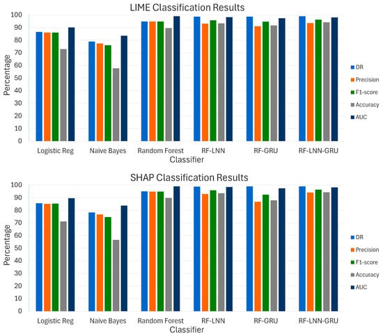
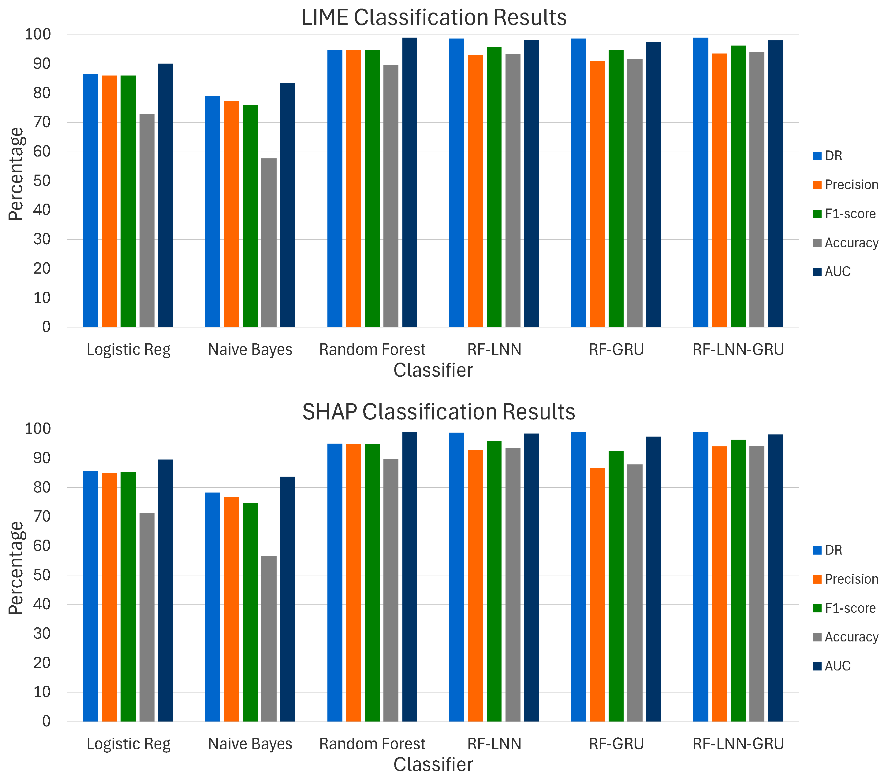
Figure 6 presents a visual comparison of model performance across six evaluation metrics. The bar chart clearly illustrates a hierarchical performance structure among the evaluated models. The proposed RF–LNN–GRU ensemble consistently achieves the highest or near-highest values across all the metrics, followed by the two-component ensembles (RF–LNN and RF–GRU), which occupy an intermediate position. Random forest represents the strongest traditional baseline, while logistic regression and naive Bayes form the lower tier of performance. The near-identical performance profiles between the LIME and SHAP feature selection methods across all the models further confirm that both XAI techniques effectively identify discriminative features, with the overlapping informative features enhancing the credibility of both approaches. This consistency demonstrates that the feature spaces selected by LIME and SHAP contain highly similar informative features, making both methods equally viable for feature distillation in Android malware detection.

Figure 6. Classification results obtained with different models.

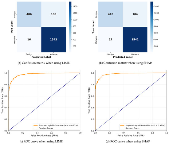
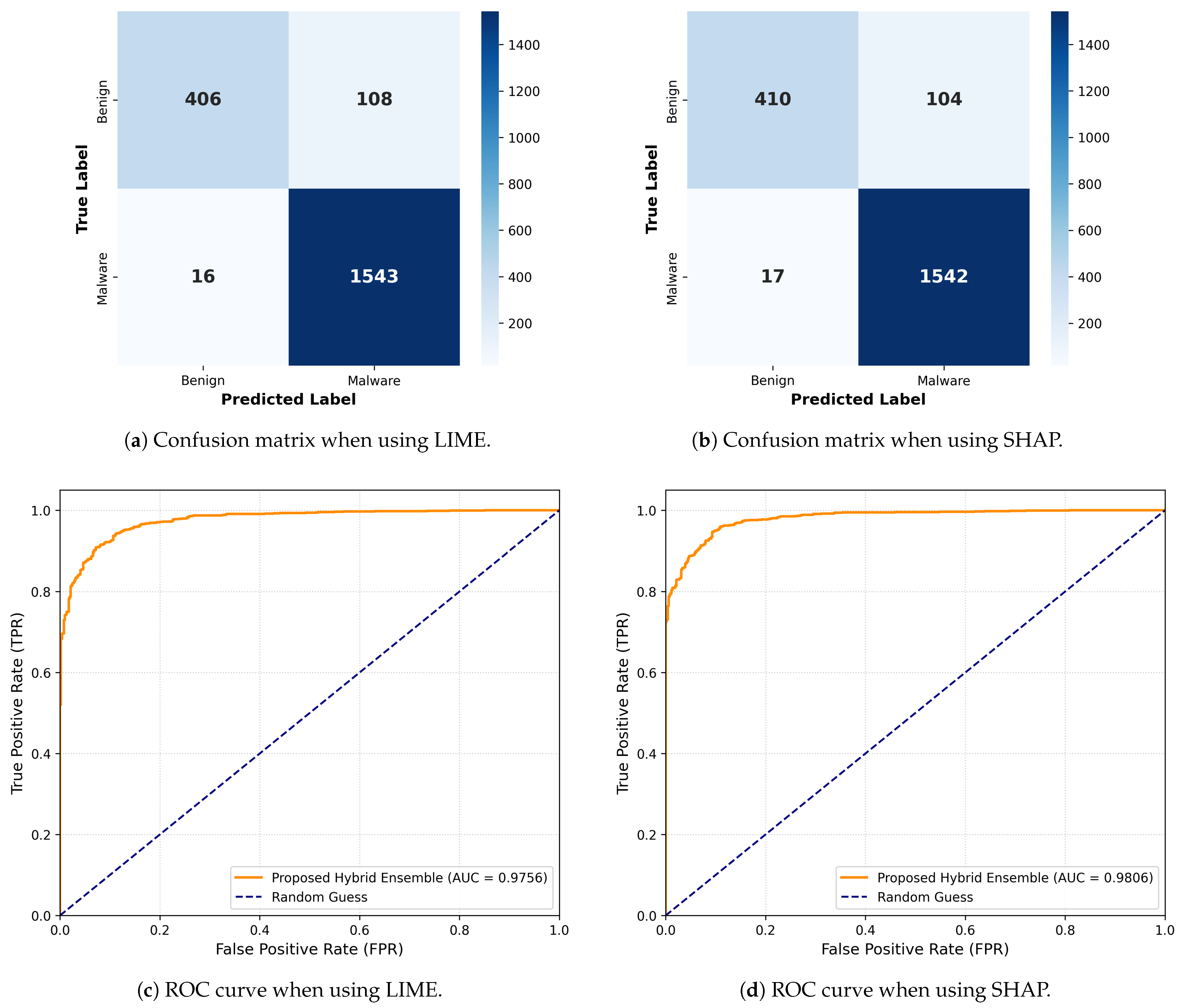
The confusion matrices and the ROC curves for the proposed model are shown in Figure 7. The confusion matrices in Figure 7a,b show that the model correctly classifies the vast majority of malware and benign samples, with only a small number of false positives and false negatives. This demonstrates the effectiveness of the selected software engineering metrics in discriminating malicious applications from benign ones. Figure 7c,d show that both feature selection methods achieve very high AUC values, confirming that the proposed framework maintains high sensitivity while keeping false alarm rates low. Although the performance of LIME and SHAP is comparable, the results show that both approaches provide highly reliable feature subsets for malware detection.

Figure 7. Confusion matrices and ROC curves of the proposed model when using LIME and SHAP.

5.6. Comparison with Other Works

This section compares our proposed model with four other models [7,8,12,38] discussed in Section 2. To provide the most meaningful comparison possible, we selected recent Android malware detection methods that satisfy the following criteria: (1) they employ datasets that fully or partially overlap with those used in this work; (2) they perform malware-versus-benign classification; (3) they target the Android platform; and (4) they report comparable performance metrics, including the detection rate. Although the experimental protocols are not identical, these criteria provide the closest basis for comparing the proposed framework with the current state of the art. In addition to the above aspects of the four works, all have been published in reputed journals: ref. [38] in the year 2026, ref. [12] in 2025, ref. [7] in 2024, and ref. [8] in 2021. Table 8 provides a comparison of the work presented in this paper with these works.

Table 8. A comprehensive comparison of the proposed model in this paper with four influential models outlined in Section 2. The time reported here includes the full pipeline time (preprocessing, training, and inference) per sample.

Model	Analysis	DR	F1	Time	Datasets (Size)	Key Features
Our Model	Static	98.98%	96.2%	<0.93 s	First Set, CICMalAnd2017, CICMalDroid2020 (10,365)	Software engineering metrics; function call graph; control flow graph; LIME and SHAP for feature selection; RF–LNN–GRU.
[38] (2026)	Dynamic	95.55%	95.15%	NR	CICMalAnd2017, CICMalDroid2020 (28,195)	Self-attention to analyze dynamic behavioral APK sequences; incremental learning; TCN.
[8] (2021)	Static	95.5%	95.44%	NR	CICMalAnd2017, CICMalDroid2020 (11,513)	Bytecode image; vectorized to a grayscale image of size 28 × 28; TCN.
[7] (2024)	Static	93.7%	94.68%	0.98 s	CICMalAnd2017, CICMalDroid2020 (19,373)	Permission-related APIs; functionality heterogeneous API graph; functionality API mapping; XGBoost.
[12] (2025)	Hybrid	93.1%	97.87%	NR	CICMalAnd2017, CICMalDroid2020 (4010)	Function name; network traffic metrics; network function call graph; network traffic graph; SVM.

The framework proposed by Rekik et al. [38] detects and mitigates Android pixnapping attacks. But the datasets used for validating their framework do not support such attacks. To overcome this limitation, the authors generated proxy pixnapping attacks.

Zhang et al. [8] also used a dataset almost identical to that used in this paper. Their model is based on a TCN classifier [54] that can outperform conventional RNNs and therefore has obtained better results than others (still less than our work) and with increased times compared to our work.

Yang et al. [7] used a set of different datasets, including the ones used in this paper. Here, we have only compared their results on the datasets CICAndMal2017 and CICMalDroid2020, which are also used in this paper. Their model is based on permission-related APIs that are generally updated when a new Android version is released. Because the framework relies on permission-related APIs, its effectiveness may be influenced by changes introduced in future Android versions. Using an MLP, a popular neural network classifier, their model achieved a DR lower than that of our model.

Feng et al. [12] used a subset of the CICAndMal2017 and CICMalDroid2020 datasets, which are also used in this paper. Their model uses a list of known, i.e., previously marked malicious functions, as one of the features. Because the proposed framework relies on structural software engineering metrics rather than predefined malicious functions, it is expected to generalize better to previously unseen malware variants. The number of samples used is less than that in our model. They used different classifiers, including MLP, to evaluate the performance of their model. The highest DR, 93.1%, achieved by their model is with the SVM classifier.

Although several of the compared studies employ advanced machine learning and deep learning techniques, many rely on computationally intensive feature representations, runtime behavioral analysis, or platform-specific artifacts such as permissions and APIs. In contrast, the proposed framework utilizes graph-derived software engineering metrics and XAI-guided feature selection to construct a compact and informative feature space. The comparative analysis indicates that this combination enables competitive or superior malware detection performance while maintaining low computational overhead and preserving interpretability.

Since the compared studies were evaluated on different dataset compositions and experimental settings, the reported results should be interpreted as indicative rather than direct performance comparisons.

Differences from the Preliminary Conference Version

As part of our discussion comparing other works, we would like to clarify that this study is a substantial extension of the work presented in the conference paper [55]. The key enhancements include: (1) the introduction of a novel model that incorporates XAI techniques, LIME, and SHAP, and a new classification, the RF–LNN–GRU model, alongside software engineering metrics to enhance classification performance; (2) an in-depth explanation and analysis of the proposed model; (3) evaluation using a significantly larger dataset yielding improved outcomes; and (4) a thorough discussion of related and future research directions.

6. Conclusions and Future Work

This paper presented a novel Android malware detection framework that combines graph-based software engineering metrics, explainable artificial intelligence (XAI), and heterogeneous ensemble learning. The proposed framework extracts structural, functional, and behavioral characteristics of Android applications from call graphs and control flow graphs (CFGs), computes statistical representations of these metrics, and employs LIME and SHAP to identify the most relevant features. The selected features are subsequently classified using the proposed RF–LNN–GRU heterogeneous ensemble model, which integrates random forest, lightweight neural networks (LNNs), and gated recurrent units (GRUs) through an asymmetric voting strategy.

The experimental evaluation on a dataset of 10,365 Android applications demonstrated the effectiveness of the proposed approach. Both LIME and SHAP successfully reduced the feature space while maintaining strong classification performance. The proposed RF–LNN–GRU model consistently outperformed traditional machine learning and ensemble baselines, achieving a detection rate of up to 98.98%, an F1-score of 96.3%, and an AUC of 98.1% while maintaining low inference latency. These results indicate that graph-derived software engineering metrics, when combined with XAI-guided feature engineering and heterogeneous ensemble learning, provide an effective and interpretable solution for Android malware detection.

Several directions remain for future research. First, additional software engineering metrics, particularly object-oriented metrics such as coupling, cohesion, inheritance, and cyclomatic complexity [14], will be investigated to further enrich the feature representation of Android applications. Second, the integration of complementary feature types, including opcode sequences, API call sequences, and other behavioral indicators, will be explored to improve detection robustness against evolving malware variants. Third, future work will investigate the combination of multiple XAI techniques to enhance feature relevance estimation and selection. In addition to local explanation methods such as LIME and SHAP, global explanation techniques, including RISE [56] and DeepLift [57], will be evaluated. Finally, the proposed framework will be extended to multiclass malware family classification and tested on larger and more diverse datasets to further assess its scalability, generalization capability, and real-world applicability.

Although the proposed framework was evaluated using a comprehensive dataset constructed from three independent Android malware repositories containing numerous malware families, categories, and obfuscated variants, the experiments were conducted using a unified dataset with random train–test partitions. A strict cross-dataset evaluation, in which the model is trained on one dataset and tested on another independent dataset, was beyond the scope of the present work. Such an evaluation would provide additional insights into the generalization capability of the proposed framework across different Android malware corpora and will be investigated in future work. Furthermore, extending the framework to other malware platforms, such as Windows executables, by incorporating platform-specific software metrics represents another promising direction for future research.

References

- Au, M.; Choo, K.K. Chapter 1—Mobile Security and Privacy. In Mobile Security and Privacy; Au, M.H., Choo, K.K.R., Eds.; Syngress: Boston, MA, USA, 2017; pp. 1–4. [Google Scholar] [CrossRef] [Scilit]
- Bhat, P.; Dutta, K. A Survey on Various Threats and Current State of Security in Android Platform. ACM Comput. Surv. 2019, 52, 21. [Google Scholar] [CrossRef] [Scilit]
- Sarker, I.H.; Furhad, M.H.; Nowrozy, R. Ai-driven cybersecurity: An overview, security intelligence modeling and research directions. SN Comput. Sci. 2021, 2, 173. [Google Scholar] [CrossRef] [Scilit]
- Chandran, S.; Syam, S.R.; Sankaran, S.; Pandey, T.; Achuthan, K. From static to ai-driven detection: A comprehensive review of obfuscated malware techniques. IEEE Access 2025, 13, 74335–74358. [Google Scholar] [CrossRef] [Scilit]
- Senanayake, J.; Kalutarage, H.; Al-Kadri, M.O. Android mobile malware detection using machine learning: A systematic review. Electronics 2021, 10, 1606. [Google Scholar] [CrossRef] [Scilit]
- Dutta, C.; Modak, S. Android malware detection using machine learning. In Proceedings of the 2025 International Conference on Artificial Intelligence for Computing, Astronomy and Renewable Energy (AICARE); IEEE: Piscataway, NJ, USA, 2025; pp. 1–5. [Google Scholar] [CrossRef] [Scilit]
- Yang, J.; Li, H.; He, L.; Xiang, T.; Jin, Y. MDADroid: A novel malware detection method by constructing functionality-API mapping. Comput. Secur. 2024, 146, 104061. [Google Scholar] [CrossRef] [Scilit]
- Zhang, W.; Luktarhan, N.; Ding, C.; Lu, B. Android malware detection using tcn with bytecode image. Symmetry 2021, 13, 1107. [Google Scholar] [CrossRef] [Scilit]
- Hossain, M.A.; Hasan, T.; Ahmed, F.; Cheragee, S.H.; Kanchan, M.H.; Haque, M.A. Towards superior android ransomware detection: An ensemble machine learning perspective. Cyber Secur. Appl. 2025, 3, 100076. [Google Scholar] [CrossRef] [Scilit]
- Tang, J.; Zhou, S.; Peng, T.; Yan, X.; Hu, X.; Tian, W. DTDroid: Adversarial Packed Android Malware Detection Based on Traffic and Dynamic Behavioral. IEEE Internet Things J. 2024, 12, 2646–2658. [Google Scholar] [CrossRef] [Scilit]
- Sharma, S.; Prachi; Chhikara, R.; Khanna, K. A novel feature selection technique: Detection and classification of Android malware. Egypt. Inform. J. 2025, 29, 100618. [Google Scholar] [CrossRef] [Scilit]
- Feng, J.; Shen, L.; Chen, Z.; Lei, Y.; Li, H. HGDetector: A hybrid Android malware detection method using network traffic and Function call graph. Alex. Eng. J. 2025, 114, 30–45. [Google Scholar] [CrossRef] [Scilit]
- Zhu, H.; Xia, M.; Wang, L.; Xu, Z.; Sheng, V.S. A Novel Knowledge Search Structure for Android Malware Detection. IEEE Trans. Serv. Comput. 2024, 17, 3052–3064. [Google Scholar] [CrossRef] [Scilit]
- Fenton, N.E.; Neil, M. Software metrics: Roadmap. In Proceedings of the Conference on the Future of Software Engineering; Association for Computing Machinery: New York, NY, USA, 2000; pp. 357–370. [Google Scholar]
- Pan, Y.; Ge, X.; Fang, C.; Fan, Y. A systematic literature review of android malware detection using static analysis. IEEE Access 2020, 8, 116363–116379. [Google Scholar] [CrossRef] [Scilit]
- Manthena, H.; Shajarian, S.; Kimmell, J.; Abdelsalam, M.; Khorsandroo, S.; Gupta, M. Explainable artificial intelligence (xai) for malware analysis: A survey of techniques, applications, and open challenges. IEEE Access 2025, 13, 61611–61640. [Google Scholar] [CrossRef] [Scilit]
- Hermosilla, P.; Berríos, S.; Allende-Cid, H. Explainable AI for Forensic Analysis: A Comparative Study of SHAP and LIME in Intrusion Detection Models. Appl. Sci. 2025, 15, 7329. [Google Scholar] [CrossRef] [Scilit]
- Alam, S.; Demir, A.K. SIFT: Sifting file types—Application of explainable artificial intelligence in cyber forensics. Cybersecurity 2024, 7, 52. [Google Scholar] [CrossRef] [Scilit]
- Tirkey, A.; Mohapatra, R.K.; Kumar, L. Policing Android Malware Using Object-Oriented Metrics and Machine Learning Techniques. In Proceedings of the Edge Analytics: Select Proceedings of 26th International Conference—ADCOM 2020; Springer: Berlin/Heidelberg, Germany, 2022; pp. 307–319. [Google Scholar]
- Tirkey, A.; Mohapatra, R.K.; Kumar, L. Anatomizing android malwares. In Proceedings of the 2019 26th Asia-Pacific Software Engineering Conference (APSEC); IEEE: Piscataway, NJ, USA, 2019; pp. 450–457. [Google Scholar]
- Blanc, W.; Hashem, L.G.; Elish, K.O.; Almohri, M.H. Identifying android malware families using android-oriented metrics. In Proceedings of the 2019 IEEE International Conference on Big Data (Big Data); IEEE: Piscataway, NJ, USA, 2019; pp. 4708–4713. [Google Scholar]
- Protsenko, M.; Müller, T. Android malware detection based on software complexity metrics. In Proceedings of the International Conference on Trust, Privacy and Security in Digital Business; Springer: Berlin/Heidelberg, Germany, 2014; pp. 24–35. [Google Scholar]
- Canfora, G.; Medvet, E.; Mercaldo, F.; Visaggio, C.A. Acquiring and analyzing app metrics for effective mobile malware detection. In Proceedings of the 2016 ACM on International Workshop on Security and Privacy Analytics; Association for Computing Machinery: New York, NY, USA, 2016; pp. 50–57. [Google Scholar]
- Liu, N.; Yang, M.; Zhang, H.; Yang, C.; Zhao, Y.; Gan, J.; Zhang, S. Detection of Android Applications with Malicious Behavior Based on Sparse Bayesian Learning Algorithm. In Proceedings of the Cloud Computing and Security: 4th International Conference, ICCCS 2018, Haikou, China, 8–10 June 2018; Springer: Berlin/Heidelberg, Germany, 2018; pp. 266–275. [Google Scholar]
- Iqubal, A.; Happy; Tiwari, S.K.; Azad, S.; Paswan, M.K. Android Based Malware Detection Technique Using Machine Learning Algorithms. In Proceedings of the 2024 First International Conference on Pioneering Developments in Computer Science & Digital Technologies (IC2SDT); IEEE: Piscataway, NJ, USA, 2024; pp. 1–6. [Google Scholar]
- Abubaker, H.; Shamsuddin, S.M.; Ali, A. Analytics on malicious android applications. Int. J. Adv. Soft Comput. Its Appl. 2018, 10, 106–118. [Google Scholar]
- Deypir, M. A new approach for effective malware detection in Android-based devices. In Proceedings of the 2016 13th International Iranian Society of Cryptology Conference on Information Security and Cryptology (ISCISC); IEEE: Piscataway, NJ, USA, 2016; pp. 112–116. [Google Scholar]
- Aswathy, A.; Amal, T.; Swathy, P.; Shojafar, M.; Vinod, P. SysDroid: A dynamic ML-based android malware analyzer using system call traces. Clust. Comput. 2020, 23, 2789–2808. [Google Scholar] [CrossRef] [Scilit]
- Dam, K.-H.T.; Touili, T. Extracting Android malicious behaviors. In Proceedings of the International Workshop on FORmal Methods for Security Engineering; SCITEPRESS: Setúbal, Portugal, 2017; Volume 2, pp. 714–723. [Google Scholar]
- Alam, S. Applying natural language processing for detecting malicious patterns in Android applications. Forensic Sci. Int. Digit. Investig. 2021, 39, 301270. [Google Scholar] [CrossRef] [Scilit]
- Mohammed, M.A.; Asante, M.; Alornyo, S.; Essah, B.O. Android applications classification with deep neural networks. Iran J. Comput. Sci. 2023, 6, 221–232. [Google Scholar] [CrossRef] [Scilit]
- Wajahat, A.; He, J.; Zhu, N.; Mahmood, T.; Nazir, A.; Ullah, F.; Qureshi, S.; Osman, M. An effective deep learning scheme for android malware detection leveraging performance metrics and computational resources. Intell. Decis. Technol. 2024, 18, 33–55. [Google Scholar] [CrossRef] [Scilit]
- El Youssofi, C.; Chougdali, K. YoloMal-XAI: Interpretable Android Malware Classification Using RGB Images and YOLO11. J. Cybersecur. Priv. 2025, 5, 52. [Google Scholar] [CrossRef] [Scilit]
- Lin, Z.; Wang, R.; Jia, X.; Zhang, S.; Wu, C. Classifying android malware with dynamic behavior dependency graphs. In Proceedings of the 2016 IEEE Trustcom/BigDataSE/ISPA; IEEE: Piscataway, NJ, USA, 2016; pp. 378–385. [Google Scholar]
- Pham, V.H.; Cam, N.T.; Duy, P.N.; Tan, N.V. RAX-ClaMal: Dynamic Android malware classification based on RAX register values. Internet Things 2025, 30, 101482. [Google Scholar] [CrossRef] [Scilit]
- Bhat, P.; Behal, S.; Dutta, K. A system call-based android malware detection approach with homogeneous & heterogeneous ensemble machine learning. Comput. Secur. 2023, 130, 103277. [Google Scholar] [CrossRef] [Scilit]
- Prasad, A.; Chandra, S.; Uddin, M.; Al-Shehari, T.; Alsadhan, N.A.; Ullah, S.S. PermGuard: A Scalable Framework for Android Malware Detection Using Permission-to-Exploitation Mapping. IEEE Access 2024, 13, 507–528. [Google Scholar] [CrossRef] [Scilit]
- Rekik, S.; Mehmood, S.; Alkhonaini, M. AdaptivePixGuard: Attention-Enhanced Temporal Convolutions for Robust Mobile Pixnapping Detection. IEEE Access 2026, 14, 34072–34095. [Google Scholar] [CrossRef] [Scilit]
- Qian, Q.; Cai, J.; Xie, M.; Zhang, R. Malicious behavior analysis for android applications. Int. J. Netw. Secur. 2016, 18, 182–192. [Google Scholar]
- Alam, S.; Altiparmak, Z. XAI-CF–Examining the Role of Explainable Artificial Intelligence in Cyber Forensics. Eng. Appl. Artif. Intell. 2026, 167, 113892. [Google Scholar] [CrossRef] [Scilit]
- Ribeiro, M.T.; Singh, S.; Guestrin, C. “Why should i trust you?” Explaining the predictions of any classifier. In Proceedings of the 22nd ACM SIGKDD International Conference on Knowledge Discovery and Data Mining; Association for Computing Machinery: New York, NY, USA, 2016; pp. 1135–1144. [Google Scholar]
- Lundberg, S.M.; Erion, G.; Chen, H.; DeGrave, A.; Prutkin, J.M.; Nair, B.; Katz, R.; Himmelfarb, J.; Bansal, N.; Lee, S.I. From local explanations to global understanding with explainable AI for trees. Nat. Mach. Intell. 2020, 2, 56–67. [Google Scholar] [CrossRef] [Scilit] [PubMed]
- Contributors. dex2jar—Tools to Work with Android .dex and Java .class Files. 2006. Available online: https://sourceforge.net/projects/dex2jar (accessed on 10 August 2026).
- Vallée-Rai, R.; Co, P.; Gagnon, E.; Hendren, L.; Lam, P.; Sundaresan, V. Soot: A Java bytecode optimization framework. In CASCON First Decade High Impact Papers; IBM Corp.: Armonk, NY, USA, 2010; pp. 214–224. [Google Scholar]
- Aho, A.V.; Lam, M.S.; Sethi, R.; Ullman, J.D. Compilers: Principles Techniques and Tools; Pearson: London, UK, 2007. [Google Scholar]
- Alam, S.; Horspool, R.N.; Traore, I.; Sogukpinar, I. A framework for metamorphic malware analysis and real-time detection. Comput. Secur. 2015, 48, 212–233. [Google Scholar] [CrossRef] [Scilit]
- Zhou, Y.; Jiang, X. Dissecting android malware: Characterization and evolution. In Proceedings of the Security and Privacy; IEEE: Piscataway, NJ, USA, 2012; pp. 95–109. [Google Scholar]
- Parkour, M. Mobile Malware Dump. 2006. Available online: http://contagiominidump.blogspot.com (accessed on 10 August 2026).
- Lashkari, A.H.; Kadir, A.F.A.; Taheri, L.; Ghorbani, A.A. Toward developing a systematic approach to generate benchmark android malware datasets and classification. In Proceedings of the 2018 International Carnahan Conference on Security Technology (ICCST); IEEE: Piscataway, NJ, USA, 2018; pp. 1–7. [Google Scholar]
- Keyes, D.S.; Li, B.; Kaur, G.; Lashkari, A.H.; Gagnon, F.; Massicotte, F. EntropLyzer: Android malware classification and characterization using entropy analysis of dynamic characteristics. In Proceedings of the 2021 Reconciling Data Analytics, Automation, Privacy, and Security: A Big Data Challenge (RDAAPS); IEEE: Piscataway, NJ, USA, 2021; pp. 1–12. [Google Scholar]
- CIC. Canadian Institute for Cybersecurity Datasets. 2026. Available online: https://www.unb.ca/cic/datasets/index.html (accessed on 10 August 2026).
- Fawcett, T. An Introduction to ROC Analysis. Pattern Recogn. Lett. 2006, 27, 861–874. [Google Scholar] [CrossRef] [Scilit]
- Sanders, R. The Pareto principle: Its use and abuse. J. Serv. Mark. 1987, 1, 37–40. [Google Scholar] [CrossRef] [Scilit]
- Bai, S.; Kolter, J.Z.; Koltun, V. An empirical evaluation of generic convolutional and recurrent networks for sequence modeling. arXiv 2018, arXiv:1803.01271. [Google Scholar]
- Alam, S.; Demir, A.K. Software Engineering Metrics For Sifting Android Malicious Applications. In Proceedings of the 1st International Conference on Innovative Engineering Sciences and Technological Research (ICIESTR); IEEE: Piscataway, NJ, USA, 2024; pp. 1–5. [Google Scholar]
- Petsiuk, V. Rise: Randomized Input Sampling for Explanation of black-box models. arXiv 2018, arXiv:1806.07421. [Google Scholar]
- Shrikumar, A.; Greenside, P.; Kundaje, A. Learning important features through propagating activation differences. In Proceedings of the International Conference on Machine Learning; PMLR: London, UK, 2017; pp. 3145–3153. [Google Scholar]
Disclaimer/Publisher’s Note: The statements, opinions and data contained in all publications are solely those of the individual author(s) and contributor(s) and not of MDPI and/or the editor(s). MDPI and/or the editor(s) disclaim responsibility for any injury to people or property resulting from any ideas, methods, instructions or products referred to in the content. |
© 2026 by the authors. Licensee MDPI, Basel, Switzerland. This article is an open access article distributed under the terms and conditions of the Creative Commons Attribution (CC BY) license.