Data-Driven Fault Diagnosis in Chemical Reactors Using Takagi–Sugeno Models and Zonotopic PI Observers

Abstract

This paper addresses fault diagnosis in nonlinear systems where reliable mathematical models are unavailable and only input–output measurements are accessible. The proposed methodology consists of three stages. First, a data-driven identification stage is performed using an Adaptive Neuro-Fuzzy Inference System (ANFIS) to capture the nonlinear dynamics of the system from fault-free sensor data. This procedure yields a set of convex Takagi–Sugeno (TS) models representing the system dynamics. In the second stage, fault detection is achieved using zonotopic proportional–integral (PI) observers with convex structures. Robustness against parametric uncertainty and sensor noise is ensured through an ${\mathcal{H}}_{\infty }$ formulation expressed as a set of linear matrix inequalities (LMIs). Finally, fault isolation is carried out using a fault signature matrix (FSM). The zonotopic framework provides adaptive set-based residual bounds that act as adaptive thresholds for fault detection, while structured residual activation patterns enable reliable fault isolation. The proposed approach is evaluated on a continuous stirred tank reactor (CSTR) under sensor faults and incipient process faults in the presence of measurement noise and compared with representative data-driven methods. Results demonstrate improved diagnostic accuracy and reduced false-alarm rates while maintaining timely fault detection and reliable isolation.

1. Introduction

Fault diagnosis (FD) of nonlinear industrial systems remains a challenging task when reliable first-principles mathematical models are unavailable or difficult to obtain. This situation is particularly common in chemical reactors, where complex nonlinear dynamics, parametric uncertainty, and measurement noise limit the applicability of classical model-based fault diagnosis techniques derived from analytical descriptions. In such scenarios, fault diagnosis strategies that rely exclusively on measured input–output data are highly desirable.

FD is an essential component to ensure the efficiency and safety of complex dynamic systems in various industrial environments. Early fault detection is critical to prevent unplanned downtimes, reduce maintenance costs, and enhance system reliability [1]. Traditionally, FD approaches have been based on control theory and statistical decision-making methods, as well as logic and optimization techniques [2]. However, the growing complexity of modern systems has driven the development of advanced methods capable of handling the uncertainties and noise inherent in real-world data.

Among model-based approaches, TS observer-based fault diagnosis schemes have received significant attention due to their ability to represent nonlinear dynamics using convex combinations of local linear models. Nevertheless, most existing TS observer designs assume that the TS model is analytically derived and that its parameters are known and fixed. This assumption significantly restricts their applicability in data-driven settings, where system dynamics must be identified from input–output measurements and are inevitably affected by modeling uncertainty.

In recent years, several data-driven methodologies have been proposed to address these challenges. Ref. [3] employed random forest algorithms and machine learning techniques to identify key state variables and improve diagnostic accuracy in complex systems. Ref. [4] developed a diagnosis approach based on comparing process measurements with optimal reference values, focusing on the analysis of temperature measurement alterations in exothermic chemical processes. Ref. [5] integrated fast Fourier transform (FFT), continuous wavelet transform (CWT), and statistical signal features to enhance fault detection across different datasets. Ref. [6] introduced the concept of cross-domain fault diagnosis (CDFD), using simulation data to train fault diagnosis models. Ref. [7] tackled fault detection in nonlinear dynamic systems using stacked neural networks and canonical variable analysis, improving robustness in systems with unknown models and nonlinearities. Ref. [8] proposed an approach for incipient fault diagnosis in nonlinear systems with stochastic uncertainties using particle filtering techniques. Ref. [9] presented a review of data-driven fault detection, focusing on three aspects: processes, study systems, and evaluation metrics. Another piece of work by [10] developed two data-driven fault detection designs for dynamic systems, validated on a three-tank system.

While data-driven methods eliminate the need for explicit mathematical models, most existing approaches focus on statistical reconstruction errors or classification accuracy and do not explicitly propagate identification-induced uncertainty into the fault diagnosis stage. As a result, their performance may degrade under measurement noise or when only limited fault-free data are available.

In the line of hybrid approach comparisons, Ref. [11] evaluated hybrid and data-driven models in catalytic reactor systems. Ref. [12] explored the use of fuzzy observers in a CSTR for fault detection, while Ref. [13] proposed a bank of linear parameter-varying (LPV) observers for actuator fault detection in chemical processes. Ref. [14] employed state observers for diagnosis in a CSTR. Comprehensive reviews of hybrid fault detection and diagnosis schemes can be found in [15,16].

On the other hand, robust model-based FD schemes have also been addressed. Ref. [17] proposed disturbance-decoupled residual generators for fault detection and isolation in nonlinear systems. Ref. [18] designed a robust observer for fault diagnosis in sensors and actuators in two series-connected CSTRs. Ref. [19] proposed a fault-tolerant control scheme based on unknown input observers, while Ref. [20] developed robust observer-based methodologies applied to CSTRs.

Despite these advances, existing robust observer-based fault diagnosis schemes rarely consider the case where the underlying TS model is obtained exclusively from data and is affected by structural uncertainty introduced during the identification process. Ignoring such uncertainty may lead to overly optimistic residual evaluation and unreliable fault detection results.

Regarding robust fault diagnosis under bounded uncertainty, set-membership and interval observer approaches have emerged as effective alternatives to conventional stochastic filters. For instance, Ref. [21] developed unknown-input observers for discrete-time TS models capable of estimating states and faults in the presence of unknown disturbances. Similarly, more recent works have proposed robust observer designs with explicit performance criteria for fault detection in discrete TS models [22], as well as interval-based state and fault estimation schemes that guarantee error bounds under bounded uncertainty [23]. While these approaches exhibit strong robustness against noise and uncertainty, they all rely on the availability of an analytically derived TS model of the system. This requirement leaves a relevant gap for applications in which only input–output measurements are available.

This work addresses the problem of achieving robust fault diagnosis for nonlinear systems using only input–output measurements, in the presence of uncertainty and measurement noise in the identified TS models.

To tackle this problem, an ANFIS is employed to structure uncertain TS models directly from fault-free input–output data, avoiding the need for analytical modeling. The resulting TS representation is then used to design zonotopic PI observers with ${\mathcal{H}}_{\infty }$ performance, which explicitly account for modeling uncertainty and measurement noise. A key advantage of the zonotopic framework is its ability to generate adaptive, set-based residual bounds that serve as decision thresholds for fault detection, rather than relying on fixed heuristic limits.

Positioning with Respect to Related Fault-Diagnosis Approaches

The literature reviewed above shows that the individual components considered in this work have been investigated separately in different fault-diagnosis contexts. Data-driven approaches avoid the need for detailed first-principles models by learning system behavior directly from available measurements [10]. Conversely, robust observer-based approaches for Takagi–Sugeno systems provide formal mechanisms for state and fault estimation under uncertainty [21,22], while interval and zonotopic techniques enable bounded state and fault estimation [23]. PI observer structures have also been studied for robust fault detection and uncertain nonlinear systems [24,25].

However, these research directions generally address data-driven identification, robust observer synthesis, and set-based uncertainty treatment as separate stages. In particular, existing TS observer-based approaches typically assume that the local models are available before observer synthesis, while conventional data-driven fault-diagnosis methods do not explicitly propagate the uncertainty introduced during model identification into a zonotopic observer and the subsequent fault-decision mechanism.

Table 1. Methodological comparison between representative fault-diagnosis approaches and the proposed framework.

Approach	Data-Driven Identification	TS/Multiple Model	Identification Uncertainty	Set-Based/ Zonotopic Estimation	PI Observer	Robust Observer Design	Adaptive Set-Based Fault Decision
Chen et al. [10]	✓	–	–	–	–	–	–
Rotondo et al. [21]	–	✓	–	–	–	✓	–
Li et al. [22]	–	✓	–	–	–	✓	–
Zhang et al. [23]	–	✓	–	✓	–	✓	∘
Shafai and Saif [24]	–	–	–	–	✓	✓	–
Orjuela et al. [25]	–	✓	–	–	✓	✓	–
Proposed framework	✓	✓	✓	✓	✓	✓	✓

✓: Explicitly addressed; ∘: partially or indirectly addressed; –: not explicitly addressed within the methodological scope considered here.

summarizes the methodological positioning of the proposed framework with respect to representative related approaches. The comparison is intended to clarify that the contribution of this work does not arise from ANFIS, TS modeling, PI observers, zonotopes, or $H_{\infty }$ synthesis individually, but from their integration into a unified data-driven fault-diagnosis framework.

In contrast with the representative approaches summarized in Table 1, the proposed methodology establishes a direct connection between data-driven nonlinear system identification, uncertainty characterization, robust set-based state estimation, and fault decision making. Nominal input–output measurements are first used to identify the nonlinear process dynamics through ANFIS. The identified consequent parameters are organized into a convex TS representation, and the uncertainty associated with the identification process is explicitly incorporated into the dynamic model. This uncertain TS representation is subsequently used to synthesize PI observer gains according to an $H_{\infty }$ robustness criterion.

The resulting zonotopic observer propagates bounded modeling uncertainty and measurement noise together with the state estimates. Consequently, fault detection does not rely on a fixed heuristic threshold; instead, it evaluates the consistency between the predicted zonotopic state enclosure and the set compatible with the current measurements. The corresponding residual activation patterns are then processed through the fault signature matrix (FSM) to perform fault isolation.

Therefore, the central methodological distinction of the proposed framework is that uncertainty arising during the data-driven identification stage is explicitly carried into the robust observer and fault-decision stages. The main contributions of this paper are summarized as follows:

• A fully data-driven fault diagnosis framework for nonlinear systems is proposed, relying exclusively on measured input–output data and avoiding the need for an analytical first-principles model.
• An ANFIS-based identification strategy is employed to construct uncertain convex TS models from fault-free measurements while explicitly accounting for identification-induced uncertainty.
• A zonotopic PI observer is developed for TS models obtained exclusively from data, integrating identification-induced uncertainty with explicit ${\mathcal{H}}_{\infty }$ robustness guarantees.
• Adaptive set-based residual bounds are generated through zonotopic state estimation, enabling fault detection based on measurement consistency rather than fixed heuristic thresholds.
• Fault isolation is performed through an FSM that exploits structured residual activation patterns, and the complete framework is validated on a CSTR considering sensor faults and incipient process faults under noisy operating conditions.

The remainder of the paper is organized as follows. Section 2 presents the proposed framework, including ANFIS-based system identification, zonotopic PI observer design, and the $H_{\infty }$ robustness conditions. Section 3 reports the identification and fault-diagnosis results and presents the comparative evaluation. Section 4 discusses the main findings, limitations, and practical implications. Finally, Section 5 summarizes the conclusions and future research directions.

Notation: In this paper, $\mathbb{N}$ and $\mathbb{R}$ denote the sets of natural and real numbers, respectively, and ${\mathbb{R}}^m$ represents the set of m-dimensional real vectors. The matrix transpose is denoted by ${(·)}^{\top }$, while $\det (·)$, $\mathrm{Tr}(·)$, and $\mathrm{Cov}(·)$ denote the determinant, trace, and covariance, respectively. The p-norm is denoted by ${\parallel ·\parallel }_p$, with ${\parallel ·\parallel }_F$ and ${\parallel ·\parallel }_{\infty }$ representing the Frobenius and infinity norms, respectively. A zonotope $\langle c,R\rangle$ is a convex set defined as $\langle c,R\rangle =\{c+R\xi :\parallel \xi {\parallel }_{\infty }\le 1\}$ [26]. If $c=0$, the zonotope is centered and remains invariant under column permutations [27]. The reduction operator ${\downarrow }_q$ limits the number of generators by retaining the most significant ones and enclosing the remaining generators [28]. The Minkowski sum and linear map of zonotopes are denoted by ⊕ and ⊙, respectively. Given two zonotopes $\langle c_1,R_1\rangle$ and $\langle c_2,R_2\rangle$, and a matrix M of appropriate dimensions, $\langle c_1,R_1\rangle \oplus \langle c_2,R_2\rangle =\langle c_1+c_2,[R_1,R_2]\rangle$, and $M\odot \langle c,R\rangle =\langle Mc,MR\rangle$. The abbreviations used throughout this work are summarized in Abbreviations.

2. Methods

2.1. Proposed Fault Diagnosis Method for Nonlinear Systems

This work considers a CSTR as a case study, a benchmark system widely used in chemical and biotechnological processes for the validation of fault diagnosis methodologies [29,30]. Although the proposed approach is validated on a CSTR, the methodology is general and can be extended to other nonlinear dynamic systems where only input–output measurements are available.

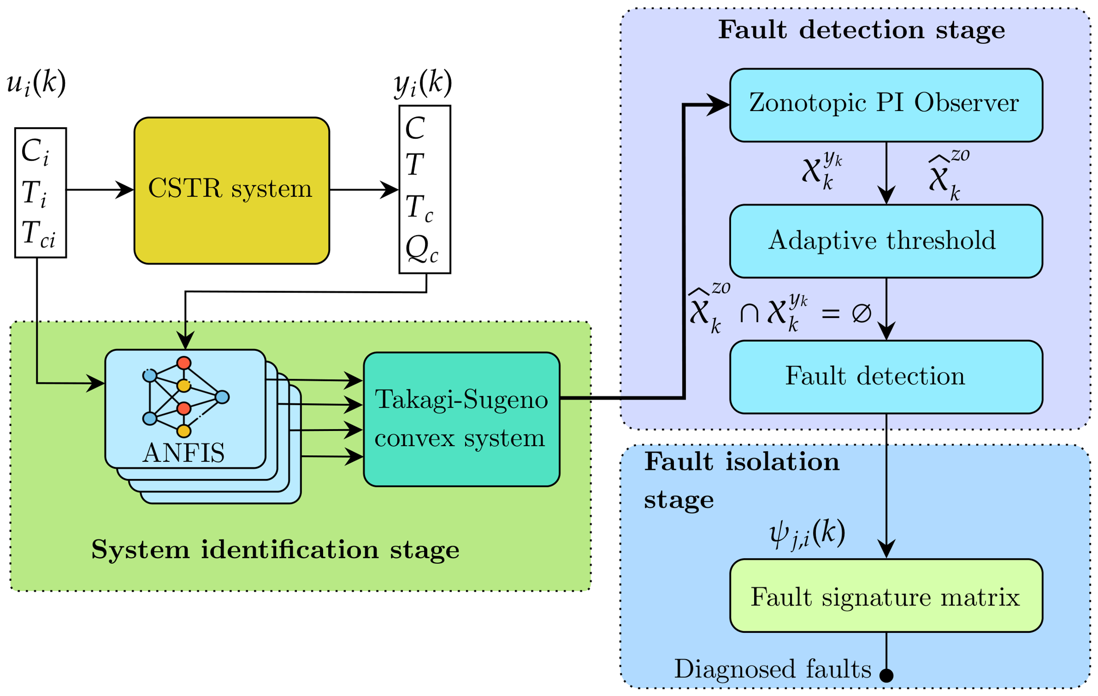
The proposed fault diagnosis method, illustrated in Figure 1, is designed for scenarios in which an explicit first-principles mathematical model of the system is unavailable or unreliable. The approach relies exclusively on measured input–output data and consists of three tightly coupled stages: data-driven system identification, uncertainty-aware fault detection, and residual-based fault isolation.

In the identification stage, an ANFIS is trained using nominal (fault-free) input–output data to capture the nonlinear dynamics of the CSTR. The ANFIS identification process is used to structure an equivalent convex TS representation of the system, avoiding analytical model derivation while explicitly accounting for identification-induced uncertainty.

Based on the identified TS models, a set of zonotopic PI observers is designed for fault detection. The observer structure explicitly incorporates modeling uncertainty and measurement noise, and robustness is guaranteed through an ${\mathcal{H}}_{\infty }$ performance criterion. At each sampling instant k, the observers generate zonotopic state estimates ${\hat{\mathcal{X}}}_k^{zo}$, which provide set-based enclosures of the true system state.

Fault detection is performed by comparing the zonotopic state estimates with measurement-consistent sets ${\mathcal{X}}_k^{y_k}$ derived from sensor readings. A fault is detected when the intersection ${\hat{\mathcal{X}}}_k^{zo}\cap {\mathcal{X}}_k^{y_k}$ becomes empty, indicating an inconsistency between the predicted system behavior and the measured data. This set-based mechanism naturally leads to adaptive detection thresholds, eliminating the need for fixed heuristic limits.

Finally, in the fault isolation stage, the activation patterns of the residuals are analyzed using a fault signature matrix (FSM). The FSM enables a logical decision process to identify the faulty component based on the structured residual responses, leading to reliable fault isolation under uncertainty and noise.

From an implementation perspective, the complete procedure is divided into offline and online stages. In the offline stage, the nominal fault-free input–output measurements are first organized into the regressive structures defined for C, T, $T_c$, and $Q_c$. Four ANFIS models are then trained to identify the corresponding nonlinear dynamics. The consequent parameters of the trained ANFIS models are arranged into the local matrices of the convex TS representation, and the associated identification uncertainty is incorporated into the uncertain model. The zonotopic PI observer gains are subsequently obtained by solving the $H_{\infty }$ LMI conditions. Once this stage is completed, the ANFIS parameters and observer gains remain fixed during online monitoring.

During the online stage, the available current and delayed measurements are used to construct the corresponding regressive vectors and evaluate the ANFIS membership functions. The normalized firing strengths determine the convex combination of the local TS submodels at each sampling instant. The zonotopic PI observers then propagate the predicted state enclosures while accounting for identification-induced uncertainty and measurement noise. For each monitored output, a measurement-consistent set is constructed and compared with the corresponding predicted zonotope. If their intersection is nonempty, the measurement is considered consistent with the predicted nominal behavior; otherwise, the associated residual is activated. Finally, the binary residual activation pattern is compared with the predefined fault signature matrix (FSM), and the corresponding fault scenario is assigned as the final diagnostic label.

2.2. Description of Data Measurements in the CSTR SYSTEM

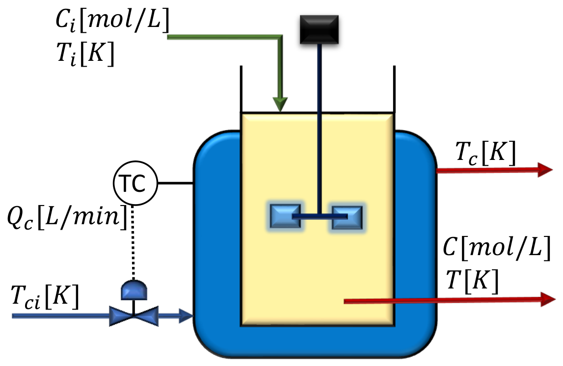
The CSTR system, shown in Figure 2, operates continuously, converting species A into species B through a second-order exothermic reaction. A cooling jacket regulates the reactor’s temperature, preventing thermal instabilities. The system has three main inputs: the inlet reactant concentration $\left(C_i\right)$, the inlet temperature $\left(T_i\right)$, and the coolant temperature $\left(T_{ci}\right)$. These inputs control the reaction rate and the heat management of the reactor. On the output side, the product concentration $\left(C\right)$, reactor temperature $\left(T\right)$, coolant temperature $\left(T_c\right)$, and coolant flow-rate $\left(Q_c\right)$ are continuously monitored to ensure optimal performance.

The simulations were generated using the “Feedback-controlled CSTR Process for Fault Simulation” benchmark, Version 1.1.0.1 [31]. The benchmark represents a three-state jacketed CSTR in which species A is converted into species B through a second-order exothermic reaction. All simulations reported in this study were executed in MATLAB/Simulink (R2025b).

The reactor operates under closed-loop temperature control. The reactor temperature T is regulated by manipulating the coolant flow rate $Q_c$ using a controller with $K_c=1.0$ and ${\tau }_I=0.2$. The manipulated coolant flow is constrained to $10\le Q_c\le 200$ L/min, and the reactor-temperature setpoint is $T_{\mathrm{sp}}=430.9$ K. The initial conditions are $C\left(0\right)=0.1$ mol/L, $T\left(0\right)=430.9$ K, and $T_c\left(0\right)=416.7$ K.

Each simulation was performed for 1200 min at a sampling rate of four samples per minute, corresponding to a data sampling interval of $T_s=15$ s and 4800 samples per measured variable. The nominal input conditions are $C_{i,0}=1$ mol/L, $T_{i,0}=350$ K, and $T_{ci,0}=350$ K. To provide excitation of the nonlinear dynamics, pseudorandom Gaussian perturbations were superimposed on the nominal inputs. The perturbation applied to $C_i$ has variance 0.002, while those applied to $T_i$ and $T_{ci}$ have variance 2. Independent seeds were generated using randi(100000).

Zero-mean Gaussian process and measurement noise were additionally included in the simulations. The process-noise generators were configured with variance ${10}^{-6}$, while the additive measurement-noise generators used variance 0.05. These values correspond to standard deviations of ${10}^{-3}$ and approximately 0.2236, respectively. The corresponding Simulink Random Number blocks use seeds generated through randi(100000) and a block sample time of 1 simulation time unit. The complete simulation, controller, initialization, input-excitation, and noise settings are summarized in

Table 2. Configuration of the CSTR benchmark and nominal data-generation conditions.

Parameter	Value	Description
Software	MATLAB/Simulink (R2025b)	Simulation environment
Reaction	Second-order exothermic	$A\to B$
Simulation time	1200 min	Duration of each simulation
Data sampling interval	15 s	Four samples/min
Samples per variable	4800	Per simulation
$C\left(0\right)$	0.1 mol/L	Initial concentration
$T\left(0\right)$	430.9 K	Initial reactor temperature
$T_c\left(0\right)$	416.7 K	Initial coolant temperature
$T_{\mathrm{sp}}$	430.9 K	Reactor-temperature setpoint
$K_c$	1.0	Controller gain
${\tau }_I$	0.2	Integral-time parameter
$Q_c$ limits	10–200 L/min	Controller-output saturation
$C_{i,0}$	1 mol/L	Nominal inlet concentration
$T_{i,0}$	350 K	Nominal inlet temperature
$T_{ci,0}$	350 K	Nominal coolant inlet temperature
$\mathrm{Var}\left(C_i\right)$	0.002	Gaussian input perturbation
$\mathrm{Var}\left(T_i\right)$	2	Gaussian input perturbation
$\mathrm{Var}\left(T_{ci}\right)$	2	Gaussian input perturbation
Process noise	$\mathcal{N}(0,{10}^{-6})$	${\sigma }_{\nu }=0.001$
Measurement noise	$\mathcal{N}(0,0.05)$	${\sigma }_{\mathrm{meas}}\approx 0.2236$
Noise-block sample time	1	Simulink Random Number blocks
Random seeds	randi(100000)	Pseudorandom realization

.

As a data-driven methodology, the proposed scheme relies on time-series information from both input and output sensors. To capture such behavior effectively, the estimation process employs a regressive structure that incorporates data from the two preceding time steps k. The output variables estimated from the inputs are organized in a regressive structure, as summarized in

Table 3. Variables to be estimated in a regressive structure.

Output ${\mathit{y}}_{\mathit{i}}$	Regressive Structure
$\hat{C}\left(k\right)$	$(C\left(k\right),C(k-1),C(k-2),C_i\left(k\right),T_i\left(k\right),T_{ci}\left(k\right))$
$\hat{T}\left(k\right)$	$(T\left(k\right),T(k-1),T(k-2),C_i\left(k\right),T_i\left(k\right),T_{ci}\left(k\right))$
${\hat{T}}_c\left(k\right)$	$(T_c\left(k\right),T_c(k-1),T_c(k-2),C_i\left(k\right),T_i\left(k\right),T_{ci}\left(k\right))$
${\hat{Q}}_c\left(k\right)$	$(Q_c\left(k\right),Q_c(k-1),Q_c(k-2),C_i\left(k\right),T_i\left(k\right),T_{ci}\left(k\right))$

.

These regressive structures act as inputs for the ANFIS, allowing them to identify the estimated variables, leading to the development of the Takagi–Sugeno convex system used for designing the zonotopic PI observer.

2.3. CSTR System Identification Using ANFIS

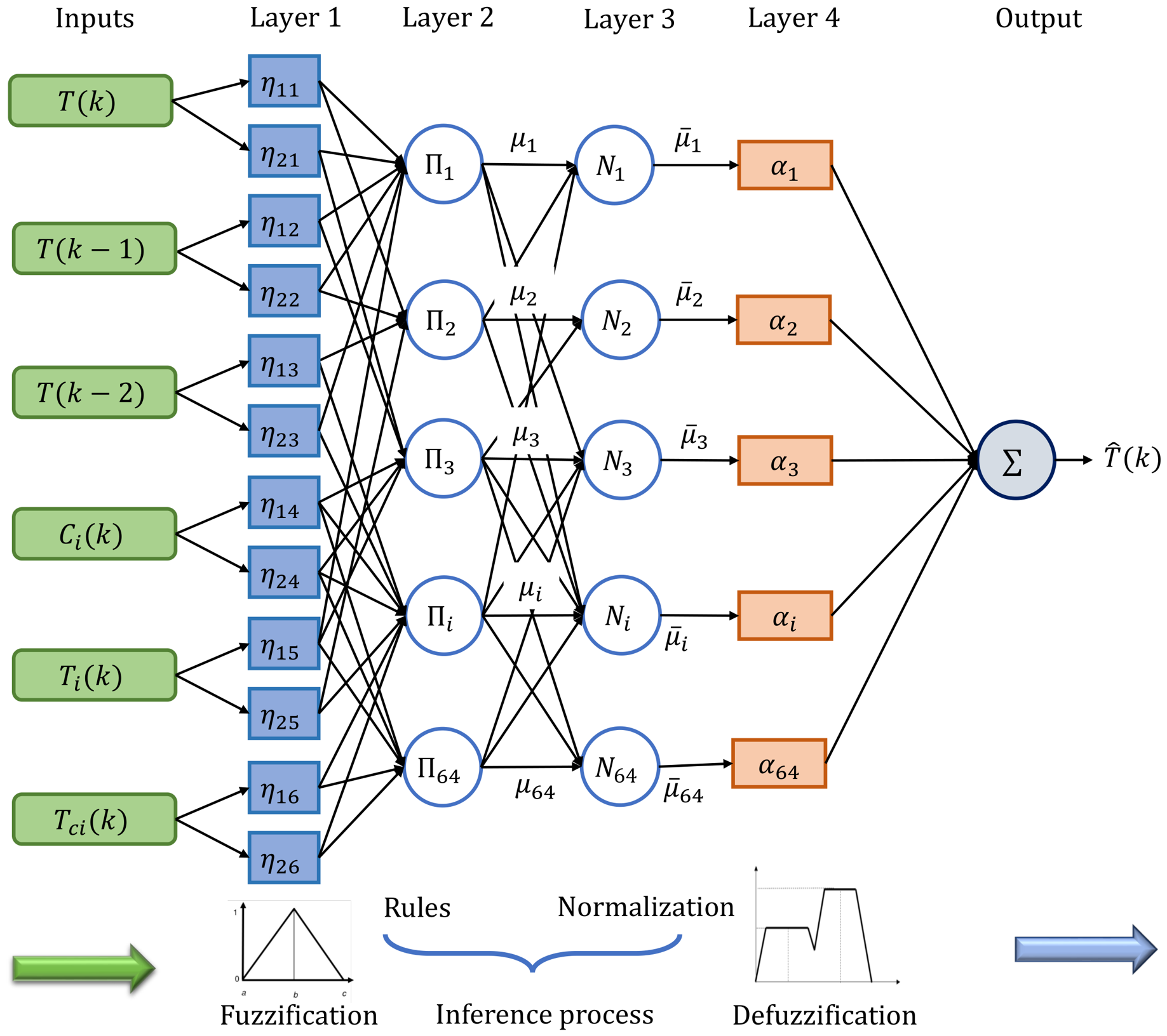
The identification of the system relies on regressive input structures, as detailed in Table 3. These inputs are arranged to match the CSTR dynamics and are processed by the ANFIS-based neural network, whose configuration is depicted in Figure 3. To ensure model fidelity, the training phase is carried out using only nominal data, free from faults. As shown in the figure, the input set comprises temperature measurements at the current and two previous time steps $T\left(k\right)$, $T(k-1)$, $T(k-2)$, along with inlet concentration $C_i\left(k\right)$, feed temperature $T_i\left(k\right)$, and coolant temperature $T_{ci}\left(k\right)$. These variables feed the fuzzy inference mechanism within the ANFIS to model system behavior and generate an estimate of the output temperature $\hat{T}\left(k\right)$.

The ANFIS framework is designed to capture the nonlinear dynamics associated with each state variable of the CSTR. As outlined in Table 3, the input vectors for the network are constructed individually for each variable, incorporating relevant temporal regressors that reflect the system’s dynamic behavior. The structure of these inputs ensures that the model effectively learns the temporal dependencies inherent to the process. Accordingly, the input vector $\zeta$ for the ANFIS is constructed by concatenating the current and past temperature values along with process inputs, as defined by

$$\zeta ={\left[\begin{array}{cccccc}T\left(k\right)& T(k-1)& T(k-2)& C_i\left(k\right)& T_i\left(k\right)& T_{ci}\left(k\right)\end{array}\right]}^{\top }.$$

(1)

The number of membership functions $N_{\mathrm{MF}}$ determines the structural complexity of the ANFIS model and was therefore treated as an identification parameter rather than as a tuning parameter of the fault-diagnosis stage. Validation-based selection of ANFIS membership-function configurations has been previously employed to assess model generalization [32]. In the present work, two membership functions were assigned to each input. As the number of fuzzy rules grows according to $N={\left(N_{\mathrm{MF}}\right)}^{N_{\zeta }}$ and each ANFIS model contains six inputs ($N_{\zeta }=6$), the adopted configuration results in $2^6=64$ fuzzy rules. Increasing $N_{\mathrm{MF}}$ to three or four would increase the rule base to $3^6=729$ and $4^6=4096$ rules, respectively, substantially increasing the number of consequent parameters to be identified and the computational burden of both the identification stage and the resulting TS representation. Therefore, $N_{\mathrm{MF}}=2$ was retained as a parsimonious configuration that provides satisfactory validation performance while maintaining a computationally tractable model complexity.

Layer 1: This layer performs the fuzzification of the input data using triangular membership functions. Two membership functions ($N_{\mathrm{MF}}=2$) are assigned to each ANFIS input. Each membership function ${\eta }_{n_f}(·)$ is parameterized by the three premise parameters $a_{n_f}$, $b_{n_f}$, and $c_{n_f}$ and is defined as

$${\eta }_{n_f}\left({\zeta }_o\right)=\left\{\begin{array}{cc}0\hfill & \mathrm{if}{\zeta }_o\le a_{n_f}\hfill \\ {\displaystyle \frac{{\zeta }_o-a_{n_f}}{b_{n_f}-a_{n_f}}}\hfill & \mathrm{if}{a}_{n_f}<{\zeta }_o\le b_{n_f}\hfill \\ {\displaystyle \frac{c_{n_f}-{\zeta }_o}{c_{n_f}-b_{n_f}}}\hfill & \mathrm{if}{b}_{n_f}<{\zeta }_o\le c_{n_f}\hfill \\ 0\hfill & \mathrm{if}{\zeta }_o>c_{n_f}\hfill \end{array}\right.,\begin{array}{c}\forall nf=1,2,\dots ,N_{\mathrm{MF}},\hfill \\ \forall o=1,2,\dots ,N_{\zeta },\hfill \end{array}$$

(2)

In the present implementation, $N_{\mathrm{MF}}=2$ triangular membership functions are assigned to each of the $N_{\zeta }=6$ regressive inputs. Therefore, the complete grid-partitioned ANFIS structure contains $N={\left(N_{\mathrm{MF}}\right)}^{N_{\zeta }}=2^6=64$ Takagi–Sugeno fuzzy rules.

Layer 2: This layer constructs the fuzzy rules by combining the outputs of the membership functions from the previous layer. Each of the $N={\left(N_{\mathrm{MF}}\right)}^{N_{\zeta }}$ nodes contains a fixed-function node that computes the firing strength of a rule by multiplying the incoming signals and forwarding the resulting product:

$$\begin{array}{c}\hfill {\mu }_i\left(\zeta \right)={\displaystyle \prod _{o=1}^{N_{\zeta }}}{\eta }_{n_f}\left({\zeta }_o\right),\forall i=1,2,\dots ,N.\end{array}$$

(3)

Layer 3: In this layer, the firing strengths obtained in Layer 2 are normalized. Each node computes the ratio between the firing strength of the i-th rule and the sum of all firing strengths, ensuring that the resulting values sum to one. These normalized values are referred to as rule weights.

$$\begin{array}{c}\hfill {\overline{\mu }}_i\left(\zeta \right)={\displaystyle \frac{{\mu }_i\left(\zeta \right)}{{\sum }_{i=1}^N{\mu }_i\left(\zeta \right)}},\forall i=1,2,\dots ,N.\end{array}$$

(4)

Layer 4: This layer calculates the contribution of each rule to the final output. Each node multiplies the normalized firing strength from Layer 3 by a linear function of the input variables. This linear function, often referred to as the consequent part of the rule, is parameterized by coefficients adjusted during training.

$$\begin{array}{c}\hfill {\mathcal{R}}_i:\mathrm{IF}{\zeta }_{1}is{\eta }_{m1}\mathrm{AND},\dots ,\mathrm{AND}{\zeta }_{N_{\zeta }}is{\eta }_{m{N}_{\zeta }}\\ \hfill \mathrm{THEN}{\overline{\mu }}_i({\zeta }_i{\alpha }_i+{\lambda }_i),\forall i=1,2,\dots ,N.\end{array}$$

(5)

Output: This layer is where the final output of the ANFIS is computed as the weighted sum of all rule contributions received from Layer 4. It aggregates all the inferred outputs into a single value representing the estimated system response.

$$\begin{array}{c}\hfill {\displaystyle \sum _{i=1}^N}{\overline{\mu }}_i({\zeta }_i{\alpha }_i+{\lambda }_i).\end{array}$$

(6)

The initial ANFIS structure was generated using grid partitioning of the six regressive input variables, with two triangular membership functions assigned to each input. This configuration results in 64 Takagi–Sugeno fuzzy rules. The initial membership functions were distributed over the ranges represented by the nominal training data.

Parameter estimation was performed using the hybrid ANFIS learning algorithm. During each training epoch, the consequent parameters were estimated through least-squares optimization, while the premise parameters of the triangular membership functions were updated through the gradient-based learning step. The initial step size was set to 0.01, with decrease and increase rates of 0.8 and 1.1, respectively. A maximum of 150 epochs was considered, and a minimum improvement of ${10}^{-4}$ was adopted as the stopping criterion.

To reduce overfitting and avoid information leakage between temporally correlated observations, the training–validation partition was performed simulation-wise. Of the 30 independent fault-free simulations, 24 complete simulations were used for training and 6 complete simulations were reserved exclusively for validation. No samples from the validation simulations were used during ANFIS parameter estimation. The complete ANFIS architecture and training configuration used for the four identified output models are summarized in

Table 4. ANFIS architecture and training configuration.

Parameter	Value
Fuzzy inference structure	Takagi–Sugeno
Inputs/output per ANFIS	6/1
Membership functions/input	2
Membership-function type	Triangular
Initialization	Grid partitioning
Number of fuzzy rules	64
Learning algorithm	Hybrid
Consequent update	Least squares
Premise update	Gradient-based
Maximum epochs	150
Minimum improvement	$1\times {10}^{-4}$
Initial step size	0.01
Step-size decrease rate	0.8
Step-size increase rate	1.1
Training runs	24
Validation runs	6
Training/validation split	Simulation-wise 80/20

.

Once the ANFIS model has been trained and both the normalized firing strengths (4) and the consequent parameters (5) have been identified, a Takagi–Sugeno (TS) fuzzy representation can be derived. As an illustrative case, the formulation of the estimated temperature variable $\hat{T}$ is presented as follows:

$$\begin{array}{c}\hfill \hat{T}\left(k\right)={\displaystyle \sum _{i=1}^N}{\overline{\mu }}_i\left(\zeta \left(k\right)\right)({\alpha }_{1i}T\left(k\right)+{\alpha }_{2i}T(k-1)+{\alpha }_{3i}T(k-2)+\\ \hfill {\alpha }_{4i}{C}_i\left(k\right)+{\alpha }_{5i}{T}_i\left(k\right)+{\alpha }_{6i}{T}_{ci}\left(k\right)+{\lambda }_i).\end{array}$$

(7)

The components of expression (7) can be reformulated and grouped as follows:

$$\begin{array}{c}\hfill \hat{T}\left(k\right)={\displaystyle \sum _{i=1}^N}{\overline{\mu }}_i\left(\zeta \left(k\right)\right)\left(\stackrel{A_i}{\overbrace{\left[\begin{array}{ccc}{\alpha }_{1i}^1& {\alpha }_{2i}^1& {\alpha }_{3i}^1\\ {\alpha }_{1i}^2& {\alpha }_{2i}^2& {\alpha }_{3i}^2\\ {\alpha }_{1i}^3& {\alpha }_{2i}^3& {\alpha }_{3i}^3\end{array}\right]}}x+\stackrel{B_i}{\overbrace{\left[\begin{array}{ccc}{\alpha }_{4i}^1& {\alpha }_{5i}^1& {\alpha }_{6i}^1\\ {\alpha }_{4i}^2& {\alpha }_{5i}^2& {\alpha }_{6i}^2\\ {\alpha }_{4i}^3& {\alpha }_{5i}^3& {\alpha }_{6i}^3\end{array}\right]}}u+\stackrel{{\lambda }_i}{\overbrace{\left[\begin{array}{c}{\lambda }_i^1\\ {\lambda }_i^2\\ {\lambda }_i^3\end{array}\right]}}\right),\end{array}$$

(8)

where $x\left(k\right)={\left[\begin{array}{ccc}T\left(k\right)& T(k-1)& T(k-2)\end{array}\right]}^T$ denotes the state vector, and $u\left(k\right)=$${\left[\begin{array}{ccc}{C}_i\left(k\right)& T_i\left(k\right)& T_{ci}\left(k\right)\end{array}\right]}^T$ denotes the input vector. The superscripts 1, 2, and 3 correspond to the ANFIS output components. The resulting polytopic model is expressed in a discrete-time state-space form as follows:

$$\begin{array}{cc}\hfill x(k+1)& ={\displaystyle \sum _{i=1}^N}{\overline{\mu }}_i\left(\zeta \left(k\right)\right)\left(A_{i}x\left(k\right)+B_{i}u\left(k\right)+{\lambda }_i\right),\hfill \\ \hfill y\left(k\right)& =Cx\left(k\right),\hfill \end{array}$$

(9)

where $N={\left(N_{\mathrm{MF}}\right)}^{N_{\zeta }}$ is the number of fuzzy rules, ${\overline{\mu }}_i\left(\zeta \left(k\right)\right)$ are the normalized firing strengths (premise functions), and the matrices $A_i\in {\mathbb{R}}^{n_x\times n_x}$, $B_i\in {\mathbb{R}}^{n_x\times n_u}$, and $C\in {\mathbb{R}}^{n_y\times n_x}$ define the system dynamics. The vector ${\lambda }_i\in {\mathbb{R}}^{n_x}$ is an affine term representing the offset learned by the ANFIS network. The output vector is given by $y\left(k\right)\in {\mathbb{R}}^{n_y}$.

Remark 1.

The convexity of the polytopic model in (9) is strictly guaranteed by the structural constraints of the ANFIS Layers 1–3. Specifically, the normalization performed in Layer 3 (see Equation (4)) ensures that the weighting functions satisfy the convex sum property: ${\sum }_{i=1}^N{\overline{\mu }}_i\left(\zeta \left(k\right)\right)=1$ and ${\overline{\mu }}_i\left(\zeta \left(k\right)\right)\ge 0$ for all $\zeta \in {\mathbb{R}}^{n_{\zeta }}$ [33]. As each ${\overline{\mu }}_i$ is derived from non-negative membership functions (2) and their T-norm product (3), the resulting firing strengths are intrinsically non-negative. This property ensures that the global nonlinear dynamics are always contained within the convex hull of the local submodels $\{A_i,B_i,{\lambda }_i\}$, providing the necessary mathematical foundation for the LMI-based stability analysis of the zonotopic observer.

It is worth noting that the CSTR system is affected by uncertainties stemming from unmodeled reaction dynamics and external disturbances. In this framework, the matrices ${\Psi }_i$ and ${\Omega }_i$ capture the parametric uncertainties associated with the dynamic model, while the matrix $F_{\sigma }$ accounts for measurement noise:

$$\begin{array}{cc}\hfill x(k+1)& ={\displaystyle \sum _{i=1}^N}{\overline{\mu }}_i\left(\zeta \left(k\right)\right)\left((A_i+{\Psi }_i)x\left(k\right)+(B_i+{\Omega }_i)u\left(k\right)+{\lambda }_i\right),\hfill \\ \hfill y\left(k\right)& =Cx\left(k\right)+F_{\sigma }\sigma \left(k\right)\hfill \end{array}$$

(10)

The uncertainty matrices ${\Psi }_i\in {\mathbb{R}}^{n_x\times n_x}$ and ${\Omega }_i\in {\mathbb{R}}^{n_x\times n_u}$ are constructed from the parameter error covariance matrix ${\mathsf{\Sigma }}_{\theta }^{\left(i\right)}$, which is obtained during the hybrid learning phase of the ANFIS model. This matrix is partitioned as follows:

$$\begin{array}{c}\hfill {\mathsf{\Sigma }}_{\theta }^{\left(i\right)}=\left[\begin{array}{ccc}{\mathsf{\Sigma }}_{A_i}& \ast & \ast \\ \ast & {\mathsf{\Sigma }}_{B_i}& \ast \\ \ast & \ast & {\mathsf{\Sigma }}_{{\lambda }_i}\end{array}\right]\end{array}$$

(11)

Here, ${\mathsf{\Sigma }}_{A_i}\in {\mathbb{R}}^{n_x^2\times n_x^2}$ and ${\mathsf{\Sigma }}_{B_i}\in {\mathbb{R}}^{n_x{n}_u\times n_x{n}_u}$ are the covariance submatrices of the consequent parameters corresponding to $A_i$ and $B_i$.

The covariance information of the consequent parameters is obtained from the least-squares stage of the hybrid ANFIS training procedure. For a given identified output, the consequent parameters associated with the ith fuzzy rule are collected as

$${\theta }_i={\left[\begin{array}{cccc}{\alpha }_{1i}& \cdots & {\alpha }_{6i}& {\lambda }_i\end{array}\right]}^{\top }.$$

(12)

Because the normalized firing strengths ${\overline{\mu }}_i\left(\zeta \left(k\right)\right)$ are fixed during the consequent-parameter update, the ANFIS output is linear with respect to the consequent parameters. Therefore, the training data can be written in regression form as

$$y=\mathsf{\Phi }\theta +e,$$

(13)

where $\mathsf{\Phi }$ is the regression matrix containing the input regressors weighted by the corresponding normalized firing strengths, $\theta$ collects the consequent parameters of all fuzzy rules, and e denotes the identification residual. After least-squares estimation, the covariance matrix of the consequent-parameter estimates is computed as

$${\mathsf{\Sigma }}_{\theta }={\hat{\sigma }}_e^2{\left({\mathsf{\Phi }}^{\top }\mathsf{\Phi }\right)}^{-1},$$

(14)

where the residual variance is estimated as

$${\hat{\sigma }}_e^2={\displaystyle \frac{{∥y-\mathsf{\Phi }\hat{\theta }∥}_2^2}{N_s-N_p}},$$

(15)

with $N_s$ denoting the number of training samples and $N_p$ the number of estimated consequent parameters. The rule-specific covariance blocks ${\mathsf{\Sigma }}_{A_i}$, ${\mathsf{\Sigma }}_{B_i}$, and ${\mathsf{\Sigma }}_{{\lambda }_i}$ are subsequently extracted according to the arrangement of the consequent parameters in the TS representation. The diagonal elements of ${\mathsf{\Sigma }}_{A_i}$ and ${\mathsf{\Sigma }}_{B_i}$ are converted into parameter-wise standard deviations and are used to construct the uncertainty matrices ${\mathsf{\Psi }}_i$ and ${\mathsf{\Omega }}_i$. To extract the uncertainty matrices, the diagonal elements (variances) are reshaped and square-rooted to obtain the standard deviations of each parameter, leading to the following:

$$\begin{array}{cc}\hfill {\mathsf{\Psi }}_i& =\mathrm{reshape}\left(\sqrt{\mathrm{diag}\left({\mathsf{\Sigma }}_{A_i}\right)},n_x,n_x\right)\hfill \end{array}$$

(16)

$$\begin{array}{cc}\hfill {\mathsf{\Omega }}_i& =\mathrm{reshape}\left(\sqrt{\mathrm{diag}\left({\mathsf{\Sigma }}_{B_i}\right)},n_x,n_u\right)\hfill \end{array}$$

(17)

Equations (16) and (17) provide the structured uncertainty matrices used in the uncertain state-space model (10), capturing the parameter-wise confidence derived from ANFIS training. The operator reshape denotes the standard transformation of a vector into a matrix of specified dimensions, consistent with column-major ordering. It is worth noting that no uncertainty is introduced in the affine term ${\lambda }_i$. This decision is justified by the fact that ${\lambda }_i$ acts as a constant offset in the model, and its influence on the system dynamics is typically negligible compared to the multiplicative terms $A_{i}x\left(k\right)$ and $B_{i}u\left(k\right)$. Furthermore, during ANFIS training, the estimation of ${\lambda }_i$ via least-squares methods tends to exhibit low variance relative to the state and input-dependent parameters. The matrix $F_{\sigma }\in {\mathbb{R}}^{n_y\times n_y}$ denotes the scaling of the additive measurement noise $\sigma \left(k\right)\in {\mathbb{R}}^{n_y}$, which reflects sensor noise affecting the CSTR output measurements.

The affine term ${\lambda }_i$ has a different role from the coefficients contained in $A_i$ and $B_i$. Once ANFIS training is completed, ${\lambda }_i$ is a fixed consequent coefficient associated with the ith local model and does not multiply either the state vector $x\left(k\right)$ or the input vector $u\left(k\right)$. Consequently, uncertainty associated with $A_i$ and $B_i$ enters the state dynamics through the multiplicative terms ${\mathsf{\Psi }}_{i}x\left(k\right)$ and ${\mathsf{\Omega }}_{i}u\left(k\right)$, respectively, while uncertainty associated with ${\lambda }_i$, if explicitly included, would enter as an additive contribution.

To quantitatively assess the relevance of this affine-term uncertainty, its propagated contribution was evaluated over the fixed validation dataset. The magnitude of the uncertainty associated with the state- and input-dependent terms was computed as

$$b_{AB}\left(k\right)={\displaystyle \sum _{i=1}^N}{\overline{\mu }}_i\left(\zeta \left(k\right)\right)\left(|{\mathsf{\Psi }}_i\left|\right|x\left(k\right)|+|{\mathsf{\Omega }}_i\left|\right|u\left(k\right)|\right),$$

(18)

while the contribution associated with the affine term was evaluated as

$$b_{\lambda }\left(k\right)={\displaystyle \sum _{i=1}^N}{\overline{\mu }}_i\left(\zeta \left(k\right)\right){\sigma }_{{\lambda }_i},{\sigma }_{{\lambda }_i}=\sqrt{\mathrm{diag}\left({\mathsf{\Sigma }}_{{\lambda }_i}\right)}.$$

(19)

The corresponding RMS uncertainty measures over the K validation samples are defined as

$$J_{AB}=\sqrt{{\displaystyle \frac{1}{K}}\sum _{k=1}^K{\parallel b_{AB}\left(k\right)\parallel }_2^2},J_{\lambda }=\sqrt{{\displaystyle \frac{1}{K}}\sum _{k=1}^K{\parallel b_{\lambda }\left(k\right)\parallel }_2^2}.$$

(20)

The relative contribution of the affine-term uncertainty is then quantified as

$${\eta }_{\lambda }=100{\displaystyle \frac{J_{\lambda }}{J_{AB}+J_{\lambda }}}.$$

(21)

Table 5. Quantitative contribution of the affine-term uncertainty in the identified ANFIS models.

Output	${\mathit{J}}_{\mathbf{AB}}$	${\mathit{J}}_{\mathit{\lambda }}$	${\mathit{\eta }}_{\mathit{\lambda }}$ (%)
C	0.0189	$1.20\times {10}^{-5}$	0.063
T	0.0274	$2.10\times {10}^{-5}$	0.077
$T_c$	0.0147	$1.00\times {10}^{-5}$	0.068
$Q_c$	0.0312	$2.80\times {10}^{-5}$	0.089

summarizes the resulting values for the four identified outputs. The affine-term uncertainty contributes less than $\mathrm{0.090\%}$ of the total propagated ANFIS uncertainty in every case, ranging from $\mathrm{0.063\%}$ for C to $\mathrm{0.089\%}$ for $Q_c$. Therefore, the dominant identification-induced uncertainty is associated with the state- and input-dependent consequent parameters contained in $A_i$ and $B_i$. These results quantitatively support retaining ${\lambda }_i$ as the fixed affine offset obtained during ANFIS training and neglecting its uncertainty in the present observer formulation.

The uncertainty matrices ${\mathsf{\Psi }}_i$ and ${\mathsf{\Omega }}_i$ are constructed from the diagonal entries of the ANFIS parameter covariance submatrices ${\mathsf{\Sigma }}_{A_i}$ and ${\mathsf{\Sigma }}_{B_i}$. This choice provides a structured and computationally tractable approximation in which each uncertain parameter is bounded individually according to its estimated variance. As a result, the uncertainty description can be directly embedded into the TS model while preserving the original dimensions of $A_i$ and $B_i$, which facilitates the subsequent zonotopic propagation and observer design.

It should be noted, however, that this approximation neglects the cross-correlations among the identified consequent parameters. Therefore, the resulting uncertainty model captures the marginal dispersion of each parameter, but not the full correlation structure encoded in the complete covariance matrix. In practical terms, this means that the proposed formulation provides a structured parameter-wise uncertainty description rather than a full statistical characterization of parameter dependence. The following section will describe the robust fault diagnosis stage based on zonotopic PI observers.

2.4. Structure of Zonotopic PI Observer

Following the approach in [34], the effect of uncertain parameters can be aggregated into a single disturbance term. Consequently, Equation (10) is reformulated as follows:

$$\begin{array}{cc}\hfill x(k+1)& ={\displaystyle \sum _{i=1}^N}{\overline{\mu }}_i\left(\zeta \left(k\right)\right)\left(A_{i}x\left(k\right)+B_{i}u\left(k\right)+{\lambda }_i+E_i\delta \left(k\right)\right),\hfill \\ \hfill y\left(k\right)& =Cx\left(k\right)+F_{\sigma }\sigma \left(k\right),\hfill \end{array}$$

(22)

with

$$\begin{array}{c}\hfill E_i\delta \left(k\right)={\Psi }_{i}x\left(k\right)+{\Omega }_{i}u\left(k\right),\end{array}$$

(23)

where $E_i$ is the uncertainty distribution matrix of suitable dimensions, and $\delta \left(k\right)\in {\mathbb{R}}^{n_x}$ is a vector that captures the impact of uncertainty.

Zonotopes are adopted due to their favorable balance between computational efficiency and expressive power for uncertainty representation. Unlike general polytopes, whose complexity grows exponentially with the system dimension, zonotopes admit a generator-based description that scales linearly. This property enables efficient computation of Minkowski sums and linear transformations, making zonotopes particularly suitable for real-time state estimation. In the proposed framework, zonotopes are used to propagate bounded disturbances and identification-induced uncertainty, allowing the construction of adaptive, set-based thresholds for robust fault detection.

A zonotope can be interpreted as a compact geometric representation of all states that are consistent with the available model and bounded uncertainty information. A zonotope $\langle c,R\rangle$ is characterized by a center c, representing the nominal or central estimate, and a generator matrix R, whose columns describe the directions and magnitudes in which the estimate may vary. Consequently, the zonotope represents a bounded set of admissible states rather than a single point estimate.

The operations used in the proposed observer have a direct geometric interpretation. A linear map transforms both the center and the generators, while a Minkowski sum combines different uncertainty contributions by augmenting the generator matrix. During recursive propagation, the number of generators may continuously increase; therefore, the inclusion-preserving operator ${\downarrow }_q$ is used to reduce the generator complexity while maintaining an outer enclosure of the original set. In the proposed framework, these operations allow identification-induced uncertainty and measurement noise to be propagated together with the estimated state. The process uncertainty and measurement noise are formally modeled using zonotopic sets, defined as follows:

$$\begin{array}{cc}\hfill \delta & \in {\mathcal{Z}}_{\delta }:=\langle c_{\delta },R_{\delta }\rangle ,\hfill \\ \hfill \sigma & \in {\mathcal{Z}}_{\sigma }:=\langle c_{\sigma },R_{\sigma }\rangle ,\hfill \end{array}$$

(24)

where $\langle c,R\rangle :=\left\{c+R\xi \mid \xi \in {\mathbb{R}}^r,{\parallel \xi \parallel }_{\infty }\le 1\right\}$ denotes a zonotope centered at c with generator matrix R. Specifically, $c_{\delta }\in {\mathbb{R}}^{n_x}$ and $c_{\sigma }\in {\mathbb{R}}^{n_y}$ are the centers of the zonotopes ${\mathcal{Z}}_{\delta }$ and ${\mathcal{Z}}_{\sigma }$ that enclose the process uncertainty and measurement noise, respectively. The corresponding generator matrices are $R_{\delta }\in {\mathbb{R}}^{n_x\times r_{\delta }}$ and $R_{\sigma }\in {\mathbb{R}}^{n_y\times r_{\sigma }}$, where $r_{\delta }$ and $r_{\sigma }$ denote the zonotope orders.

The zonotopic observer is initialized from a bounded set centered at the nominal initial state. Specifically,

$${\hat{\mathcal{X}}}_0^{zo}=〈c_0^{zo},R_0^{zo}〉,$$

(25)

with

$$c_0^{zo}=\left[\begin{array}{c}0.100\\ 430.9\\ 416.7\end{array}\right],R_0^{zo}=\left[\begin{array}{ccc}0.005& 0& 0\\ 0& 1.0& 0\\ 0& 0& 1.0\end{array}\right].$$

(26)

Accordingly, the initial state is assumed to satisfy $C\left(0\right)\in [0.095,0.105]$ mol/L, $T\left(0\right)\in [429.9,431.9]$ K, and $T_c\left(0\right)\in [415.7,417.7]$ K. This nonzero initial generator matrix accounts for a small bounded uncertainty around the nominal initial condition and prevents the observer from starting from an artificially exact point estimate.

To enhance state estimation in the presence of persistent disturbances and modeling uncertainties, a discrete-time PI observer structure is developed within the TS framework. This formulation extends the conventional proportional observer by incorporating an integral action on the output estimation error, thereby improving robustness and sensitivity to incipient faults.

Although PI observer structures have been previously studied in the literature, the following development is specifically tailored to TS models obtained exclusively from input–output data. In contrast to classical formulations, the proposed observer is embedded within a zonotopic framework and incorporates ${\mathcal{H}}_{\infty }$ robustness to explicitly handle identification-induced uncertainty and measurement noise. Following the design methodology proposed by [24], the PI observer is formulated as follows:

$$\begin{array}{cc}\hfill \hat{x}(k+1)& ={\displaystyle \sum _{i=1}^N}{\overline{\mu }}_i\left(\zeta \left(k\right)\right)\left(A_i\hat{x}\left(k\right)+B_{i}u\left(k\right)+{\lambda }_i+L_{P,i}\left(y\left(k\right)-\hat{y}\left(k\right)\right)+L_{I,i}\eta \left(k\right)\right),\hfill \end{array}$$

(27)

$$\begin{array}{cc}\hfill \eta (k+1)& =\eta \left(k\right)+y\left(k\right)-\hat{y}\left(k\right),\hfill \end{array}$$

(28)

$$\begin{array}{cc}\hfill \hat{y}\left(k\right)& =C\hat{x}\left(k\right),\hfill \end{array}$$

(29)

where $\hat{x}\left(k\right)\in {\mathbb{R}}^{n_x}$ is the estimated state vector, $\eta \left(k\right)\in {\mathbb{R}}^{n_y}$ is the integral state, which accumulates the output estimation error over time, $\hat{y}\left(k\right)=C\hat{x}\left(k\right)$ is the estimated system output, $L_{P,i}$ and $L_{I,i}$ are the proportional and integral observer gains associated with the i-th submodel, and ${\overline{\mu }}_i\left(\zeta \left(k\right)\right)$ are the normalized activation functions determined by the scheduling vector $\zeta \left(k\right)$.

Unlike classical PI observer formulations, the proposed structure operates on zonotopic state enclosures derived from data-driven TS models, enabling adaptive, set-based residual generation under bounded uncertainty.

This structure also facilitates the synthesis of observer gains via LMIs, ensuring robust convergence of the estimation error dynamics under bounded uncertainty and noise.

It is emphasized that the PI observer structure itself is not claimed to be novel; rather, the contribution lies in its integration with data-driven TS modeling, zonotopic state estimation, and ${\mathcal{H}}_{\infty }$-based robustness guarantees.

This formulation is a generalization of the PI observer introduced in [24,25] to the case of fuzzy TS models with multiple submodels and nonlinear weighting.

The error is obtained from the relation $e\left(k\right)=x\left(k\right)-\hat{x}\left(k\right)$, and the error dynamic $e(k+1)$ is

$$e(k+1)=x(k+1)-\hat{x}(k+1),$$

(30)

From the definition of the estimation error in (30), and by substituting the system (22) and observer (27) into this relation, the error dynamics can be expressed as follows:

$$\begin{array}{c}\hfill e(k+1)={\displaystyle \sum _{i=1}^N}{\displaystyle \sum _{j=1}^N}{\overline{\mu }}_i\left(\zeta \left(k\right)\right){\overline{\mu }}_j\left(\zeta \left(k\right)\right)\left[(A_i-L_{P,j}C)e\left(k\right)+E_i\delta \left(k\right)-L_{P,j}{F}_{\sigma }\sigma \left(k\right)-L_{I,j}\eta \left(k\right)\right]\end{array}$$

(31)

The integral state is updated as follows:

$$\begin{array}{cc}\hfill \eta (k+1)& =\eta \left(k\right)+y\left(k\right)-\hat{y}\left(k\right)\hfill \\ \hfill & =\eta \left(k\right)+Ce\left(k\right)+F_{\sigma }\sigma \left(k\right)\hfill \end{array}$$

(32)

Thus, the extended error dynamics become

$$\begin{array}{c}\hfill \tilde{e}(k+1)={\displaystyle \sum _{i=1}^N}{\displaystyle \sum _{j=1}^N}{\overline{\mu }}_i\left(\zeta \left(k\right)\right){\overline{\mu }}_j\left(\zeta \left(k\right)\right)\left(\underset{{\mathcal{A}}_{ij}}{\underbrace{\left[\begin{array}{cc}{A}_i-L_{P,j}C& -L_{I,j}\\ C& I\end{array}\right]}}\tilde{e}\left(k\right)+\underset{{\mathcal{B}}_{ij}}{\underbrace{\left[\begin{array}{cc}{E}_i& -L_{P,j}{F}_{\sigma }\\ 0& F_{\sigma }\end{array}\right]}}{\varphi }_w\left(k\right)\right)\end{array}$$

(33)

with the extended state vector:

$$\tilde{e}\left(k\right)=\left[\begin{array}{c}e\left(k\right)\\ \eta \left(k\right)\end{array}\right],{\varphi }_w\left(k\right)=\left[\begin{array}{c}\delta \left(k\right)\\ \sigma \left(k\right)\end{array}\right]$$

(34)

Finally, the complete extended error dynamics can be written as

$$\tilde{e}(k+1)={\displaystyle \sum _{i=1}^N}{\displaystyle \sum _{j=1}^N}{\overline{\mu }}_i\left(\zeta \left(k\right)\right){\overline{\mu }}_j\left(\zeta \left(k\right)\right)\left({\mathcal{A}}_{ij}\tilde{e}\left(k\right)+{\mathcal{B}}_{ij}{\varphi }_w\left(k\right)\right)$$

(35)

where

$$\begin{array}{cc}\hfill {\mathcal{A}}_{ij}& =\left[\begin{array}{cc}{A}_i-L_{P,j}C& -L_{I,j}\\ C& I\end{array}\right],{\mathcal{B}}_{ij}=\left[\begin{array}{cc}{E}_i& -L_{P,j}{F}_{\sigma }\\ 0& F_{\sigma }\end{array}\right]\hfill \end{array}$$

(36)

The extended error dynamics in (35) provide the basis for the subsequent ${\mathcal{H}}_{\infty }$ LMI-based synthesis of the zonotopic PI observer gains, explicitly accounting for identification-induced uncertainty and measurement noise in a data-driven TS framework.

A zonotopic observer that encloses the system states under uncertainty (22) can be expressed as ${\hat{\mathcal{X}}}_k=\langle c_k^x,R_k^x\rangle$, derived from the observer formulation (27) and Proposition 1, assuming bounded uncertainties and zonotopic representation under the following assumption.

Proposition 1.

Given the uncertain TS system (22) and the PI observer (27), with bounded disturbances ${\delta }_k\in \langle 0,I_{n_{\delta }}\rangle$ and noise ${\sigma }_k\in \langle 0,I_{n_{\sigma }}\rangle$, the predicted zonotope ${\hat{\mathcal{X}}}_{k+1}^{zo}=\langle c_{k+1}^{zo},R_{k+1}^{zo}\rangle$ is

$$c_{k+1}^{zo}={\displaystyle \sum _{i=1}^N}{\overline{\mu }}_i\left(\zeta \left(k\right)\right)\left[(A_i-L_{P,i}C)c_k^{zo}+B_i{u}_k+{\lambda }_i+L_{P,i}{y}_k+L_{I,i}\eta \left(k\right)\right],$$

(37)

$$R_{k+1}^{zo}=\left[\left({\displaystyle \sum _{i=1}^N}{\overline{\mu }}_i\left(\zeta \left(k\right)\right)(A_i-L_{P,i}C)\right){\overline{R}}_k^{zo},\left({\displaystyle \sum _{i=1}^N}{\overline{\mu }}_i\left(\zeta \left(k\right)\right)E_i\right),-\left({\displaystyle \sum _{i=1}^N}{\overline{\mu }}_i\left(\zeta \left(k\right)\right)L_{P,i}{F}_{\sigma }\right)\right],$$

(38)

$${\overline{R}}_k^{zo}={\downarrow }_q\left(R_k^{zo}\right),$$

(39)

where ${\downarrow }_q(·)$ is an inclusion-preserving generator reduction to fixed order q.

Proof. 

Let $\hat{x}\left(k\right)\in {\hat{\mathcal{X}}}_k^{zo}=\langle c_k^{zo},R_k^{zo}\rangle$ with the reduced form ${\overline{R}}_k^{zo}{=\downarrow }_q\left(R_k^{zo}\right)$. From the PI-TS observer, for each submodel i we have

$$\begin{array}{c}\hfill \hat{x}(k+1)=(A_i-L_{P,i}C)\hat{x}\left(k\right)+B_i{u}_k+{\lambda }_i+L_{P,i}{y}_k+L_{I,i}\eta \left(k\right)+E_i{\delta }_k-L_{P,i}{F}_{\sigma }{\sigma }_k,\end{array}$$

(40)

weighted by ${\overline{\mu }}_i\left(\zeta \left(k\right)\right)$ and summed over i.

We propagate sets using standard zonotope operations: (i) Linear map: $M\odot \langle c,R\rangle =\langle Mc,MR\rangle$; (ii) Minkowski sum: $\langle c_1,R_1\rangle \oplus \langle c_2,R_2\rangle =\langle c_1+c_2,\left[R_1{R}_2\right]\rangle$; and (iii) Scalar multiplication: $\kappa \odot \langle c,R\rangle =\langle \kappa c,\kappa R\rangle$ with $\kappa \ge 0$.

We apply (i)–(iii) term by term for a fixed i:

$$(A_i-L_{P,i}C)\odot \langle c_k^{zo},{\overline{R}}_k^{zo}\rangle =\langle (A_i-L_{P,i}C)c_k^{zo},(A_i-L_{P,i}C){\overline{R}}_k^{zo}\rangle ,$$

(41)

$$B_i\odot \langle u_k,0\rangle =\langle B_i{u}_k,0\rangle ,$$

(42)

$$\langle {\lambda }_i,0\rangle ,$$

(43)

$$L_{P,i}\odot \langle y_k,0\rangle =\langle L_{P,i}{y}_k,0\rangle ,$$

(44)

$$\langle L_{I,i}\eta \left(k\right),0\rangle ,$$

(45)

$$E_i\odot \langle 0,I_{n_{\delta }}\rangle =\langle 0,E_i\rangle ,$$

(46)

$$(-L_{P,i}{F}_{\sigma })\odot \langle 0,I_{n_{\sigma }}\rangle =\langle 0,-L_{P,i}{F}_{\sigma }\rangle .$$

(47)

Deterministic terms such as (42)–(45) contribute only to the zonotope center, while terms (41), (46) and (47) contribute to the generator matrix. We then combine these contributions via Minkowski sum (ii), and weight them by ${\overline{\mu }}_i\left(\zeta \left(k\right)\right)$ using (iii). As ${\sum }_{i=1}^N{\overline{\mu }}_i\left(\zeta \left(k\right)\right)=1$ and ${\overline{\mu }}_i\ge 0$, the convex combination of centers and the linearity of the image yield

$${\displaystyle \sum _{i=1}^N}{\overline{\mu }}_i\left(\zeta \left(k\right)\right)(A_i-L_{P,i}C)\odot \langle c_k^{zo},{\overline{R}}_k^{zo}\rangle =\left({\displaystyle \sum _{i=1}^N}{\overline{\mu }}_i\left(\zeta \left(k\right)\right)(A_i-L_{P,i}C)\right)\odot \langle c_k^{zo},{\overline{R}}_k^{zo}\rangle ,$$

(48)

which produces the first block in (37) and (38) by (i). Similarly, as the same uncertainty ${\delta }_k$ and noise ${\sigma }_k$ affect all submodels,

$${\displaystyle \sum _{i=1}^N}{\overline{\mu }}_i\left(\zeta \left(k\right)\right)\langle 0,E_i\rangle =〈0,{\displaystyle \sum _{i=1}^N}{\overline{\mu }}_i\left(\zeta \left(k\right)\right)E_i〉,$$

(49)

$${\displaystyle \sum _{i=1}^N}{\overline{\mu }}_i\left(\zeta \left(k\right)\right)\langle 0,-L_{P,i}{F}_{\sigma }\rangle =〈0,-{\displaystyle \sum _{i=1}^N}{\overline{\mu }}_i\left(\zeta \left(k\right)\right)L_{P,i}{F}_{\sigma }〉,$$

(50)

which form the second and third blocks in (38). The deterministic terms $B_i{u}_k$, ${\lambda }_i$, $L_{P,i}{y}_k$, and $L_{I,i}\eta \left(k\right)$ only shift the center (no new generators are added), yielding (37). Finally, the reduction operator ${\downarrow }_q$ in (39) preserves set inclusion while bounding complexity.

Therefore, ${\hat{\mathcal{X}}}_{k+1}^{zo}=\langle c_{k+1}^{zo},R_{k+1}^{zo}\rangle$ is given by (37)–(39).    □

Note from expression (38) that the deterministic terms $\langle {\lambda }_i,0\rangle$, $(B_i\odot \langle u_k,0\rangle )$, $(L_{P,i}\odot \langle y_k,0\rangle )$, and $(L_{I,i}\eta \left(k\right),0)$ have no impact on the generator matrix $R_{k+1}^{zo}$ and influence only the center $c_{k+1}^{zo}$ of the zonotope $\langle c_{k+1}^{zo},R_{k+1}^{zo}\rangle$. Assuming that the estimated state belongs to the zonotope ${\hat{\mathcal{X}}}_k^{zo}=\langle c_k^{zo},R_k^{zo}\rangle$, with its reduced generator matrix ${\overline{R}}_k^{zo}{=\downarrow }_q\left(R_k^{zo}\right)$, and that the disturbances and noise are bounded as ${\delta }_k\in \langle 0,I_{n_{\delta }}\rangle$ and ${\sigma }_k\in \langle 0,I_{n_{\sigma }}\rangle$, the estimation error $e\left(k\right)=x\left(k\right)-\hat{x}\left(k\right)$ is enclosed at the next step by the zonotope:

$$e(k+1)\in \langle 0,R_{k+1}^e\rangle ,$$

(51)

with the generator matrix given by

$$R_{k+1}^e=\left[\left({\displaystyle \sum _{i=1}^N}{\overline{\mu }}_i\left(\zeta \left(k\right)\right)(A_i-L_{P,i}C)\right){\overline{R}}_k^{zo},\left({\displaystyle \sum _{i=1}^N}{\overline{\mu }}_i\left(\zeta \left(k\right)\right)E_i\right),-\left({\displaystyle \sum _{i=1}^N}{\overline{\mu }}_i\left(\zeta \left(k\right)\right)L_{P,i}{F}_{\sigma }\right)\right].$$

(52)

To ensure robustness against bounded disturbances and measurement noise, the observer gains $L_{P,i}$ and $L_{I,i}$ are designed according to an ${\mathcal{H}}_{\infty }$ performance criterion. The goal is to minimize the worst-case amplification from the disturbance input to the estimation error by solving a convex optimization problem subject to LMI constraints.

The reduction order q is an implementation parameter of the zonotopic propagation and is independent of the LMI-based $H_{\infty }$ observer synthesis. Its purpose is to prevent the continuous growth of the number of generators during recursive set propagation while preserving an outer enclosure of the estimated set. In all simulations, the reduction order was fixed to $q=15$. For the considered observers, the state dimension is $n_x=3$; hence, this setting corresponds to a maximum reduced generator budget equal to five times the state dimension. The selected value was adopted as a practical compromise between retaining geometric information in the zonotopic representation and maintaining bounded computational complexity. No optimality claim is made regarding $q=15$. A systematic optimization of the reduction order is not addressed in the present work and constitutes a possible direction for future investigation.

For the CSTR implementation, the normalized disturbance and measurement-noise variables satisfy $\parallel {\delta }_k{\parallel }_{\infty }\le 1$ and $\parallel {\sigma }_k{\parallel }_{\infty }\le 1$, respectively. Their actual magnitudes are introduced through the uncertainty-distribution and measurement-noise scaling matrices

$$E=\left[\begin{array}{ccc}0.039& 0& 0\\ 0& 0.042& 0\\ 0& 0& 0.040\end{array}\right],F_{\sigma }=\left[\begin{array}{ccc}0.662& 0& 0\\ 0& 0.679& 0\\ 0& 0& 0.667\end{array}\right].$$

(53)

Consequently, the bounded model-uncertainty contribution satisfies the componentwise bounds $\left|E{\delta }_k\right|\le {[0.039,0.042,0.040]}^{\top }$, while the bounded measurement-noise contribution satisfies $|F_{\sigma }{\sigma }_k|\le {[0.662,0.679,0.667]}^{\top }$. Equivalently, $\parallel E{\delta }_k{\parallel }_{\infty }\le 0.042$ and $\parallel F_{\sigma }{\sigma }_k{\parallel }_{\infty }\le 0.679$. These bounds are propagated explicitly through the zonotopic observer at each sampling instant.

2.5. Robust Zonotopic PI Observer Design

To ensure that the uncertain TS system (22), identified exclusively from data, and the proposed zonotopic PI observer (27) achieve convergence, the origin of the extended error dynamics (35) must be asymptotically stable. The objective is to derive sufficient conditions that guarantee ${\mathcal{H}}_{\infty }$ robustness of the estimation error dynamics in the presence of identification-induced uncertainty and measurement noise. These conditions are summarized in the following theorem.

Theorem 1.

Consider the discrete-time TS system subject to additive uncertainty and measurement noise, together with the proposed zonotopic PI observer designed for TS models obtained from input–output data. For a prescribed disturbance attenuation level $\gamma >0$, the extended error system (35) satisfies the ${\mathcal{H}}_{\infty }$ performance criterion with attenuation index γ if there exist a symmetric positive-definite matrix $P\in {\mathbb{R}}^{n\times n}$, design matrices $Y_j,W_j\in {\mathbb{R}}^{n\times p}$, and a scalar $\overline{\gamma }={\gamma }^2$, such that the following inequality holds for all $(i,j)\in \{1,2,\dots ,N\}$:

$${\displaystyle \frac{2}{N-1}}{\mathcal{L}}_{ii}+{\mathcal{L}}_{ij}+{\mathcal{L}}_{ji}<0,$$

(54)

where the matrix ${\mathcal{L}}_{ij}$ is defined as

$${\mathcal{L}}_{ij}=\left[\begin{array}{cccc}{C}^{\top }C-P& C^{\top }{E}_w& {\tilde{A}}_{ij}^{\top }P& {\tilde{B}}_{ij}^{\top }P\\ E_w^{\top }C& E_w^{\top }{E}_w-\overline{\gamma }I& 0& 0\\ P{\tilde{A}}_{ij}& 0& P& 0\\ P{\tilde{B}}_{ij}& 0& 0& \overline{\gamma }I\end{array}\right],$$

(55)

with

$$\begin{array}{cc}\hfill {\tilde{A}}_{ij}& =\left[\begin{array}{cc}{A}_i-Y_{j}C{P}^{-1}& -W_j{P}^{-1}\\ C& I\end{array}\right],\hfill \end{array}$$

(56)

$$\begin{array}{cc}\hfill {\tilde{B}}_{ij}& =\left[\begin{array}{cc}{E}_i& -Y_j{F}_{\sigma }{P}^{-1}\\ 0& F_{\sigma }\end{array}\right].\hfill \end{array}$$

(57)

Then, the designed observer ensures the internal stability of the extended error dynamics and guarantees that the ${\mathcal{H}}_{\infty }$ performance criterion

$${\displaystyle \sum _{k=0}^{\infty }}{r}^{\top }\left(k\right)r\left(k\right)<{\gamma }^2{\displaystyle \sum _{k=0}^{\infty }}{\varphi }_w^{\top }\left(k\right){\varphi }_w\left(k\right)$$

(58)

is satisfied for all admissible disturbances. Taking into account that ${\gamma }^2=\overline{\gamma }$, the zonotopic condition

$${\parallel e\left(k\right)\parallel }_2^2<{\gamma }^2{\parallel {\varphi }_w\left(k\right)\parallel }_2^2$$

(59)

is fulfilled, and the corresponding LMI conditions are derived using the Schur complement and convex relaxation.

Proof. 

Let $V\left(k\right)={\tilde{e}}^{\top }\left(k\right)P\tilde{e}\left(k\right)$ be the Lyapunov candidate function with $P>0$. The extended error dynamics are given by

$$\tilde{e}(k+1)={\tilde{A}}_{ij}\tilde{e}\left(k\right)+{\tilde{B}}_{ij}{\varphi }_w\left(k\right),$$

(60)

and the residual is defined as

$$r\left(k\right)=Ce\left(k\right)+E_w{\varphi }_w\left(k\right),$$

(61)

where $E_w=\left[\begin{array}{cc}0& -F_{\sigma }\end{array}\right]$ and ${\varphi }_w\left(k\right)=\left[\begin{array}{c}\delta \left(k\right)\\ \sigma \left(k\right)\end{array}\right]$ is the disturbance vector that includes process and measurement uncertainty.

The ${\mathcal{H}}_{\infty }$ performance condition is expressed as

$$J_{r1}=\mathsf{\Delta }V(k+1)+r^{\top }\left(k\right)r\left(k\right)-{\gamma }^2{\varphi }_w^{\top }\left(k\right){\varphi }_w\left(k\right)<0.$$

(62)

We expand $\mathsf{\Delta }V(k+1)$ as

$$\begin{array}{cc}\hfill \mathsf{\Delta }V(k+1)& ={({\tilde{A}}_{ij}\tilde{e}\left(k\right)+{\tilde{B}}_{ij}{\varphi }_w\left(k\right))}^{\top }P({\tilde{A}}_{ij}\tilde{e}\left(k\right)+{\tilde{B}}_{ij}{\varphi }_w\left(k\right))-{\tilde{e}}^{\top }\left(k\right)P\tilde{e}\left(k\right)\hfill \end{array}$$

(63)

$$\begin{array}{cc}\hfill & ={\left[\begin{array}{c}\tilde{e}\left(k\right)\\ {\varphi }_w\left(k\right)\end{array}\right]}^{\top }\left[\begin{array}{cc}{\tilde{A}}_{ij}^{\top }P{\tilde{A}}_{ij}-P& {\tilde{A}}_{ij}^{\top }P{\tilde{B}}_{ij}\\ {\tilde{B}}_{ij}^{\top }P{\tilde{A}}_{ij}& {\tilde{B}}_{ij}^{\top }P{\tilde{B}}_{ij}\end{array}\right]\left[\begin{array}{c}\tilde{e}\left(k\right)\\ {\varphi }_w\left(k\right)\end{array}\right].\hfill \end{array}$$

(64)

For the residual term:

$$r^{\top }\left(k\right)r\left(k\right)-{\gamma }^2{\varphi }_w^{\top }\left(k\right){\varphi }_w\left(k\right)={\left[\begin{array}{c}\tilde{e}\left(k\right)\\ {\varphi }_w\left(k\right)\end{array}\right]}^{\top }\left[\begin{array}{cc}{C}^{\top }C& C^{\top }{E}_w\\ E_w^{\top }C& E_w^{\top }{E}_w-{\gamma }^{2}I\end{array}\right]\left[\begin{array}{c}\tilde{e}\left(k\right)\\ {\varphi }_w\left(k\right)\end{array}\right].$$

(65)

Adding both contributions, we define the total inequality:

$$J_{r1}={\left[\begin{array}{c}\tilde{e}\left(k\right)\\ {\varphi }_w\left(k\right)\end{array}\right]}^{\top }{\mathcal{L}}_{ij}\left[\begin{array}{c}\tilde{e}\left(k\right)\\ {\varphi }_w\left(k\right)\end{array}\right]<0,$$

(66)

with

$${\mathcal{L}}_{ij}=\left[\begin{array}{cc}{C}^{\top }C-P+{\tilde{A}}_{ij}^{\top }P{\tilde{A}}_{ij}& C^{\top }{E}_w+{\tilde{A}}_{ij}^{\top }P{\tilde{B}}_{ij}\\ E_w^{\top }C+{\tilde{B}}_{ij}^{\top }P{\tilde{A}}_{ij}& E_w^{\top }{E}_w-{\gamma }^{2}I+{\tilde{B}}_{ij}^{\top }P{\tilde{B}}_{ij}\end{array}\right].$$

(67)

Applying the Schur complement, and defining $L_{P,j}=Y_j{P}^{-1}$ and $L_{I,j}=W_j{P}^{-1}$, the inequality becomes a convex LMI in variables P, $Y_j$, and $W_j$.

Using the convex relaxation from [33], the term

$${\displaystyle \sum _{i=1}^N}{\displaystyle \sum _{j=1}^N}{\overline{\mu }}_i\left(\zeta \left(k\right)\right){\overline{\mu }}_j\left(\zeta \left(k\right)\right){\mathcal{L}}_{ij}$$

(68)

is upper-bounded by

$${\displaystyle \frac{2}{N-1}}{\mathcal{L}}_{ii}+{\mathcal{L}}_{ij}+{\mathcal{L}}_{ji},$$

(69)

which yields tractable LMIs. Taking into account ${\gamma }^2=\overline{\gamma }$, the zonotopic condition

$${\parallel e\left(k\right)\parallel }_2^2<{\gamma }^2{\parallel {\varphi }_w\left(k\right)\parallel }_2^2$$

is satisfied. This concludes the proof.    □

Remark 2.

Rather than selecting the attenuation level γ empirically, the observer synthesis can be formulated as the following convex optimization problem:

$$\begin{array}{cc}\hfill \underset{P,Y_j,W_j,\overline{\gamma }}{\mathrm{minimize}}& \overline{\gamma }\hfill \\ \hfill \mathrm{subject}\mathrm{to}& P\succ 0,\hfill \\ \hfill & {\displaystyle \frac{2}{N-1}}{\mathcal{L}}_{ii}+{\mathcal{L}}_{ij}+{\mathcal{L}}_{ji}\prec 0,\forall (i,j),\hfill \end{array}$$

(70)

where $\overline{\gamma }={\gamma }^2$. Therefore, ${\gamma }^{\star }=\sqrt{{\overline{\gamma }}^{\star }}$ represents the smallest disturbance-attenuation level admitted by the proposed LMI conditions. The optimization is performed offline, and the observer gains $L_{P,j}=Y_j{P}^{-1}$ and $L_{I,j}=W_j{P}^{-1}$ obtained from the solution are subsequently fixed for online implementation.

For the numerical implementation, the LMI conditions of Theorem 1 were formulated in MATLAB (R2025b) using YALMIP as the optimization modeling interface and solved with the SeDuMi 1.3 semidefinite-programming solver. To numerically enforce the strict matrix inequalities, a feasibility margin of $\epsilon ={10}^{-8}$ was adopted. Accordingly, each strict LMI condition $\mathcal{L}<0$ was implemented as

$$\mathcal{L}⪯-\epsilon I,\epsilon ={10}^{-8}.$$

(71)

The ${\mathcal{H}}_{\infty }$ disturbance-attenuation bound was minimized subject to the complete set of LMI feasibility constraints. The resulting optimization problem was feasible, and yielded

$$\gamma =0.8452.$$

(72)

Once a feasible solution $(P,Y_i,W_i)$ is obtained, the proportional and integral observer gains are recovered using the same variable transformations introduced in the proof of Theorem 1:

$$L_{P,i}=Y_i{P}^{-1},L_{I,i}=W_i{P}^{-1},i=1,\dots ,N.$$

(73)

For the present ANFIS-derived TS representation, $N=64$ local models are considered. The complete numerical set of proportional and integral observer gains used in the simulations is reported in Appendix A.

The LMI optimization is performed only once during the offline observer-design stage, after the ANFIS-based TS model and its uncertainty description have been obtained. The resulting matrices P, $Y_i$, and $W_i$, and, consequently, the gains ${\mathcal{L}}_i$, remain fixed throughout online operation. Therefore, no semidefinite optimization problem is solved at each sampling instant. During online operation, only the normalized activation weights ${\overline{\mu }}_i\left(\zeta \left(k\right)\right)$ are updated according to the current scheduling variables, and the corresponding precomputed local observer contributions are combined through the Takagi–Sugeno interpolation mechanism.

The main numerical settings employed for the ${\mathcal{H}}_{\infty }$ observer synthesis are summarized in

Table 6. Numerical configuration of the ${\mathcal{H}}_{\infty }$ LMI observer synthesis.

Parameter	Setting
Software environment	MATLAB (R2025b)
Optimization interface	YALMIP
Semidefinite solver	SeDuMi 1.3
Feasibility margin $\epsilon$	$1\times {10}^{-8}$
Optimal attenuation $\gamma$	0.8452
Number of TS local models	64
LMI synthesis	Offline
Online LMI solution	No
Online gain recomputation	No

.

2.6. Fault Detection and Isolation Stage

The FD procedure based on zonotopic PI observers combines state estimation from the ANFIS with uncertainty and noise propagation handled by the zonotopic framework. Faults are detected by verifying whether the estimated zonotope intersects the measurement strip at each time step. A fault is flagged whenever this intersection is empty, indicating inconsistency between prediction and measurement. For each residual channel s, fault detection is performed without introducing a manually tuned fixed threshold. Let the predicted zonotope at time k be ${\hat{\mathcal{X}}}_k^{zo}=\langle c_k^{zo},R_k^{zo}\rangle$, and let $C_s$ denote the measurement row associated with the sth residual. The projection of the predicted zonotope onto the corresponding measurement direction is the interval

$${\mathcal{Y}}_s^{zo}\left(k\right)=\left[C_s{c}_k^{zo}-\parallel C_s{R}_k^{zo}{\parallel }_1,C_s{c}_k^{zo}+{\parallel C_s{R}_k^{zo}\parallel }_1\right].$$

(74)

The measurement-consistent interval is defined as

$${\mathcal{Y}}_s^m\left(k\right)=\left[y_s\left(k\right)-{\nu }_s,y_s\left(k\right)+{\nu }_s\right],$$

(75)

where ${\nu }_s$ is the corresponding measurement-noise bound obtained from $F_{\sigma }{\mathcal{Z}}_{\sigma }$. Hence, the adaptive residual threshold is

$${\tau }_s\left(k\right)={\parallel C_s{R}_k^{zo}\parallel }_1+{\nu }_s.$$

(76)

Using the residual

$$r_s\left(k\right)=y_s\left(k\right)-C_s{c}_k^{zo},$$

(77)

the binary residual activation is computed as

$${\psi }_s\left(k\right)=\left\{\begin{array}{cc}0,\hfill & |r_s\left(k\right)|\le {\tau }_s\left(k\right),\hfill \\ 1,\hfill & |r_s\left(k\right)|>{\tau }_s\left(k\right).\hfill \end{array}\right.$$

(78)

Numerically, the set-intersection test is therefore implemented as an interval-overlap test. The predicted and measurement-consistent intervals intersect if and only if

$$\max \left\{C_s{c}_k^{zo}-{\parallel C_s{R}_k^{zo}\parallel }_1,y_s\left(k\right)-{\nu }_s\right\}\le \min \left\{C_s{c}_k^{zo}+{\parallel C_s{R}_k^{zo}\parallel }_1,y_s\left(k\right)+{\nu }_s\right\}.$$

(79)

Accordingly, an empty intersection is equivalently detected when

$${\hat{\mathcal{X}}}_k^{zo}\cap {\mathcal{X}}_k^{y_s}=\varnothing ⟺\left|r_s\left(k\right)\right|>{\tau }_s\left(k\right).$$

(80)

Thus, no additional linear or nonlinear optimization problem is required for the online intersection test. The decision is obtained directly from the center and generator matrix of the propagated zonotope and the prescribed measurement-noise bound. For fault isolation, the binary residual vector is defined as

$$\psi \left(k\right)={\left[\begin{array}{cccc}{\psi }_1\left(k\right)& {\psi }_2\left(k\right)& {\psi }_3\left(k\right)& {\psi }_4\left(k\right)\end{array}\right]}^{\top }.$$

(81)

The predefined fault signature matrix used in the CSTR case study is

$${\mathcal{M}}_{\mathrm{FSM}}=\left[\begin{array}{cccccc}1& 0& 0& 0& 1& 0\\ 0& 1& 0& 0& 1& 0\\ 0& 0& 1& 0& 1& 1\\ 0& 0& 0& 1& 0& 1\end{array}\right],$$

(82)

where the rows correspond to residuals $(r_1,r_2,r_3,r_4)$ and the columns correspond to fault scenarios $(f_1,\dots ,f_6)$. Fault isolation is performed by comparing the observed binary signature $\psi \left(k\right)$ with the columns of ${\mathcal{M}}_{\mathrm{FSM}}$. An exact match with column j assigns fault $f_j$, while $\psi \left(k\right)=0$ corresponds to nominal operation.

The set of candidate fault scenarios is defined a priori according to the physical faults considered in the CSTR benchmark. However, the binary entries of the FSM are obtained offline from dedicated single-fault simulations rather than being assigned solely from process knowledge. For each fault scenario $f_j$, the zonotopic detection procedure is applied and the corresponding residual activation pattern is recorded. Specifically, the FSM entry is defined as

$${\psi }_{s,j}=\left\{\begin{array}{cc}1,\hfill & \mathrm{if}\mathrm{residual}{r}_s\mathrm{is}\mathrm{inconsistent}\mathrm{under}\mathrm{fault}{f}_j,\hfill \\ 0,\hfill & \mathrm{otherwise},\hfill \end{array}\right.$$

(83)

where inconsistency is determined through the adaptive set-based criterion $|r_s\left(k\right)|>{\tau }_s\left(k\right)$. Thus, the candidate fault set is specified from process knowledge, while the residual signatures forming the FSM are derived from the simulated fault responses. No additional statistical or machine-learning classifier is used to construct the FSM. During online fault isolation, let $\psi \left(k\right)$ denote the observed binary residual signature and let $m_j$ denote the jth column of ${\mathcal{M}}_{\mathrm{FSM}}$. The set of candidate faults compatible with the observed signature is defined as

$$\mathcal{J}\left(k\right)=\left\{j\in \{1,\dots ,N_f\}:\psi \left(k\right)=m_j\right\}.$$

(84)

The isolation decision is then defined as follows:

$$\mathcal{D}\left(k\right)=\left\{\begin{array}{cc}\mathrm{nominal},\hfill & \psi \left(k\right)=0,\hfill \\ f_j,\hfill & \left|\mathcal{J}\right(k\left)\right|=1,\hfill \\ \mathrm{ambiguous}/\mathrm{unisolated},\hfill & \left|\mathcal{J}\right(k\left)\right|\ne 1\mathrm{and}\psi \left(k\right)\ne 0.\hfill \end{array}\right.$$

(85)

Accordingly, a fault label is assigned only when the observed residual signature uniquely matches one column of the FSM. A nonzero signature that does not provide a unique match is retained as an ambiguous diagnostic event rather than being forcibly assigned to one of the predefined fault classes.

The present FSM was constructed and validated for single-fault scenarios. Simultaneous faults are therefore not assumed to be uniquely isolable by the current matrix. If two faults $f_a$ and $f_b$ occur simultaneously, a first logical approximation to the resulting residual signature would be the element-wise Boolean union,

$$m_{a,b}=m_a\vee m_b,$$

(86)

where ∨ denotes the element-wise logical OR operation. However, such a combined signature is not necessarily unique, and nonlinear interactions between simultaneous faults may further modify the residual response. Consequently, simultaneous-fault isolation is not guaranteed by the current FSM. Its systematic treatment would require augmenting ${\mathcal{M}}_{\mathrm{FSM}}$ with dedicated combined-fault signatures and performing an isolability analysis for the enlarged fault set.

The complete online fault-detection and isolation procedure, including zonotope propagation, adaptive residual evaluation, numerical intersection testing, and FSM-based fault isolation, is summarized in Algorithm 1.

Algorithm 1 Zonotopic fault detection and isolation scheme

Require:  Measured inputs $u\left(k\right)$ and outputs $y\left(k\right)$; ANFIS-derived TS models ${\{A_i,B_i,{\lambda }_i,{\overline{\mu }}_i\}}_{i=1}^N$; precomputed observer gains ${\{L_{P,i},L_{I,i}\}}_{i=1}^N$; initial zonotope ${\hat{\mathcal{X}}}_0^{zo}=\langle c_0^{zo},R_0^{zo}\rangle$; reduction order $q=15$; ${\mathcal{Z}}_{\delta }=\langle 0,I_3\rangle$; ${\mathcal{Z}}_{\sigma }=\langle 0,I_3\rangle$; uncertainty matrices $E_i$ and $F_{\sigma }$; ${\gamma }_{\mathrm{opt}}=0.8452$; and fault signature matrix ${\mathcal{M}}_{\mathrm{FSM}}$. Ensure:  Fault-detection decision and isolated fault label.    1: Initialize ${\hat{\mathcal{X}}}_0^{zo}=\langle c_0^{zo},R_0^{zo}\rangle$ and the integral observer state $\eta \left(0\right)$.    2: for each sampling instant k do    3:       Evaluate the ANFIS membership functions and compute the normalized TS weights ${\overline{\mu }}_i\left(\zeta \left(k\right)\right)$.    4:       Propagate the zonotopic PI observer using the precomputed gains $L_{P,i}$ and $L_{I,i}$.    5:       Reduce the generator matrix as ${\overline{R}}_k^{zo}{=\downarrow }_q\left(R_k^{zo}\right)$, with $q=15$.    6:       for each residual channel $s=1,\dots ,4$ do    7:             Compute the residual $r_s\left(k\right)=y_s\left(k\right)-C_s{c}_k^{zo}$.    8:             Compute the projected zonotope half-width $h_s\left(k\right)={\parallel C_s{R}_k^{zo}\parallel }_1$.    9:             Obtain the measurement-noise bound ${\nu }_s$ from $F_{\sigma }{\mathcal{Z}}_{\sigma }$.  10:             Compute the adaptive threshold ${\tau }_s\left(k\right)=h_s\left(k\right)+{\nu }_s$.  11:             if $|r_s\left(k\right)|>{\tau }_s\left(k\right)$ then  12:                ${\psi }_s\left(k\right)\leftarrow 1$                 ▹ empty intersection  13:             else  14:                ${\psi }_s\left(k\right)\leftarrow 0$                 ▹ nonempty intersection  15:             end if  16:       end for  17:       Form the binary residual signature $\psi \left(k\right)={[{\psi }_1\left(k\right),{\psi }_2\left(k\right),{\psi }_3\left(k\right),{\psi }_4\left(k\right)]}^{\top }$.  18:       if $\psi \left(k\right)=0$ then  19:             Declare nominal operation.  20:       else  21:             Compare $\psi \left(k\right)$ with the columns of ${\mathcal{M}}_{\mathrm{FSM}}$.  22:             if $\psi \left(k\right)={\mathcal{M}}_{\mathrm{FSM}}(:,j)$ for a unique j then  23:                Isolate fault $f_j$.  24:             else  25:                Report an unclassified residual signature.  26:             end if  27:       end if  28: end for

It is noted that $\gamma =0.8452$ is an offline observer-design parameter used to obtain the fixed gains $L_{P,i}$ and $L_{I,i}$ through the ${\mathcal{H}}_{\infty }$ LMI synthesis. It is reported among the algorithm parameters for reproducibility, but the LMI problem and $\gamma$ are not recomputed during online diagnosis. The generation of residuals $r_s$ relies on the estimated variables presented in Table 3, and specialized zonotopic PI observers will be developed specifically for tracking these residuals:

$$\begin{array}{cc}\hfill r_1\left(k\right)& =C\left(k\right)-\hat{C}\left(k\right),\hfill \end{array}$$

(87)

$$\begin{array}{cc}\hfill r_2\left(k\right)& =T\left(k\right)-\hat{T}\left(k\right),\hfill \end{array}$$

(88)

$$\begin{array}{cc}\hfill r_3\left(k\right)& =T_c\left(k\right)-{\hat{T}}_c\left(k\right),\hfill \end{array}$$

(89)

$$\begin{array}{cc}\hfill r_4\left(k\right)& =Q_c\left(k\right)-{\hat{Q}}_c\left(k\right),\hfill \end{array}$$

(90)

3. Results

In this section, the results of the proposed hybrid method for fault diagnosis using ANFIS and zonotopic PI observers are presented. The method was evaluated on a CSTR model simulator specifically configured for this purpose.

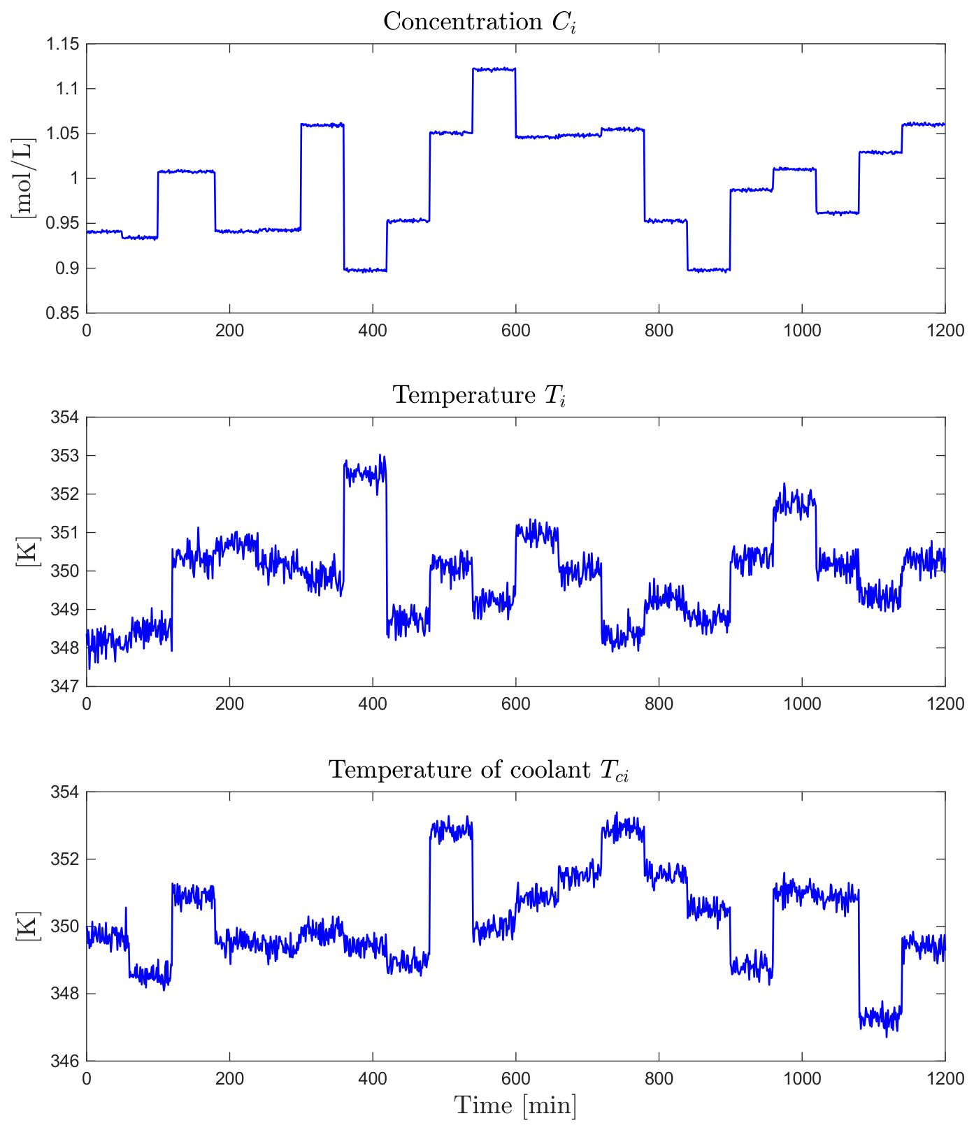
The CSTR system was subjected to several tests under different operating conditions, with 30 simulations conducted in fault-free scenarios. The simulation time was $1200 \min$ with four samples per minute. The Simulink benchmark includes random number generator blocks to perturb the inputs $\left[\begin{array}{ccc}{C}_i& T_i& T_{ci}\end{array}\right]$, along with process noise and added sensor noise. This allows the numerical simulations to have random variations around their nominal values, as shown in Figure 4. Input perturbations reveal complex system dynamics, leading to temporally correlated measurements and non-Gaussian distributions due to the inherent nonlinearity of the process.

A total of 30 independent fault-free simulations were generated for ANFIS identification and validation. Each simulation was performed for 1200 min at a sampling rate of four samples per minute, resulting in 4800 samples per simulation. To prevent information leakage between temporally correlated samples belonging to the same trajectory, the training–validation partition was performed simulation-wise rather than by randomly splitting individual samples. Specifically, 24 complete simulations (80%) were assigned to the training dataset and the remaining six complete simulations (20%) were reserved exclusively for validation. Consequently, the training and validation sets contained 115,200 and 28,800 samples, respectively. The same validation simulations were maintained throughout all subsequent analyses.

The ANFIS models were trained for 150 epochs using the nominal training partition.

Table 7. Training and validation RMSE of the identified ANFIS models.

Output	Training RMSE	Validation RMSE
C	$3.8971\times {10}^{-4}$	$4.1683\times {10}^{-4}$
T	$4.7316\times {10}^{-4}$	$5.0827\times {10}^{-4}$
$T_c$	$5.8462\times {10}^{-4}$	$6.2149\times {10}^{-4}$
$Q_c$	$6.9623\times {10}^{-4}$	$7.3816\times {10}^{-4}$

reports the identification accuracy for each output variable. Training root mean square error (RMSE) ranged from $3.8971\times {10}^{-4}$ to $6.9623\times {10}^{-4}$, while validation RMSE ranged from $4.1683\times {10}^{-4}$ to $7.3816\times {10}^{-4}$. In all four cases, the validation error remains close to the corresponding training error, indicating that the identified models preserve their predictive performance on simulations that were not used during parameter estimation. The RMSE is defined as

$$RMSE=\sqrt{{\displaystyle \frac{1}{N_{\iota }}}\sum _{\iota =1}^{N_{\iota }}{(y_{\iota }-{\hat{y}}_{\iota })}^2}$$

(91)

where $y_{\iota }$ and ${\hat{y}}_{\iota }$ denote the measured and predicted values, respectively, and $N_{\iota }$ is the number of observations used for the corresponding training or validation evaluation.

3.1. Influence of Training-Data Availability

As the proposed methodology constructs the uncertain TS representation from ANFIS models identified exclusively from nominal data, the amount of available training information can influence the accuracy of the subsequent diagnostic model. To investigate this effect while preserving complete independence of the validation data, a simulation-wise sensitivity analysis was performed.

The six simulations originally assigned to the validation dataset were kept fixed in all experiments. The amount of training information was varied by using 6, 12, 18, and 24 complete nominal simulations, corresponding to 25%, 50%, 75%, and 100% of the original training partition, respectively. As each simulation contains 4800 samples, these configurations correspond to 28,800, 57,600, 86,400, and 115,200 training samples. No sample from the fixed validation simulations was used during ANFIS training. The simulation-wise configurations used to evaluate the sensitivity to the amount of nominal training data are summarized in

Table 8. Simulation-wise configurations used to evaluate sensitivity to the amount of nominal training data.

Training Fraction	Training Runs	Samples/Run	Training Samples
25%	6	4800	28,800
50%	12	4800	57,600
75%	18	4800	86,400
100%	24	4800	115,200

.

Table 9. Sensitivity of ANFIS validation performance to the amount of nominal training data.

Training Fraction	${\mathbf{RMSE}}_{\mathbf{C}}$	${\mathbf{RMSE}}_{\mathbf{T}}$	${\mathbf{RMSE}}_{{\mathbf{T}}_{\mathbf{c}}}$	${\mathbf{RMSE}}_{{\mathbf{Q}}_{\mathbf{c}}}$
25%	$6.2847\times {10}^{-4}$	$7.0912\times {10}^{-4}$	$8.3564\times {10}^{-4}$	$9.6183\times {10}^{-4}$
50%	$5.0379\times {10}^{-4}$	$6.0216\times {10}^{-4}$	$7.1258\times {10}^{-4}$	$8.3971\times {10}^{-4}$
75%	$4.4261\times {10}^{-4}$	$5.3478\times {10}^{-4}$	$6.5182\times {10}^{-4}$	$7.7249\times {10}^{-4}$
100%	$4.1683\times {10}^{-4}$	$5.0827\times {10}^{-4}$	$6.2149\times {10}^{-4}$	$7.3816\times {10}^{-4}$

presents the validation RMSE obtained for each output as the amount of nominal training data is progressively increased. Importantly, all RMSE values were computed using the same six previously unseen validation simulations, so that differences among the configurations are attributable exclusively to the amount of information available during ANFIS identification.

A consistent reduction in validation error is observed as the number of training simulations increases. Relative to the 25% training configuration, using the complete training partition reduces the validation RMSE by approximately 33.7%, 28.3%, 25.6%, and 23.3% for C, T, $T_c$, and $Q_c$, respectively. This confirms that strongly reducing the amount of nominal training information deteriorates the accuracy of the identified models.

The improvement becomes progressively smaller as additional training simulations are incorporated. In particular, increasing the training partition from 75% to 100% reduces the validation RMSE by only approximately 5.8%, 5.0%, 4.7%, and 4.4% for C, T, $T_c$, and $Q_c$, respectively. This behavior indicates diminishing improvements once the principal nominal process dynamics are sufficiently represented in the identification dataset.

To further assess the repeatability of the identification performance, the RMSE was computed independently for each of the 30 fault-free simulations.

Table 10. Run-wise ANFIS identification accuracy across the 30 independent fault-free simulations.

Output	RMSE (Mean ± SD)
C	$(3.9477\pm 0.2048)\times {10}^{-4}$
T	$(4.8545\pm 0.2491)\times {10}^{-4}$
$T_c$	$(5.1915\pm 0.5783)\times {10}^{-4}$
$Q_c$	$(7.0389\pm 0.3675)\times {10}^{-4}$

reports the resulting mean and standard deviation of the run-wise RMSE for each identified output. The results show consistent prediction accuracy across the independent nominal realizations, with $T_c$ exhibiting the largest run-to-run variability among the four outputs.

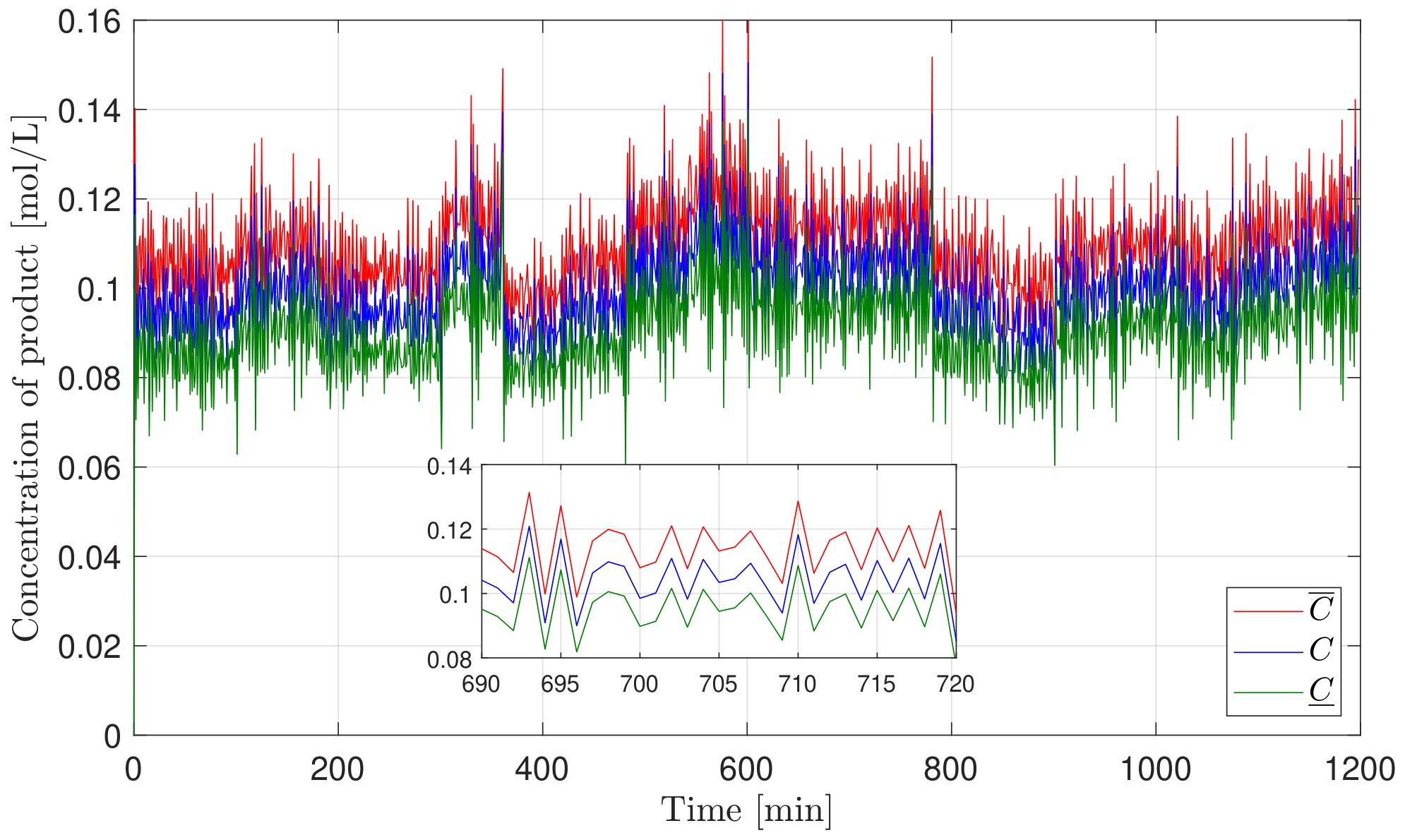
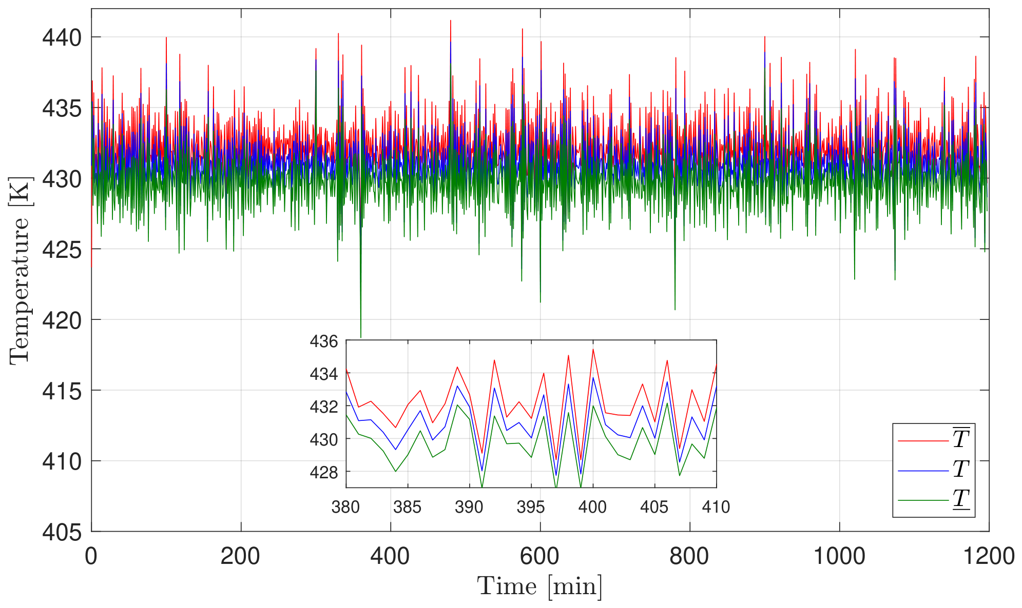
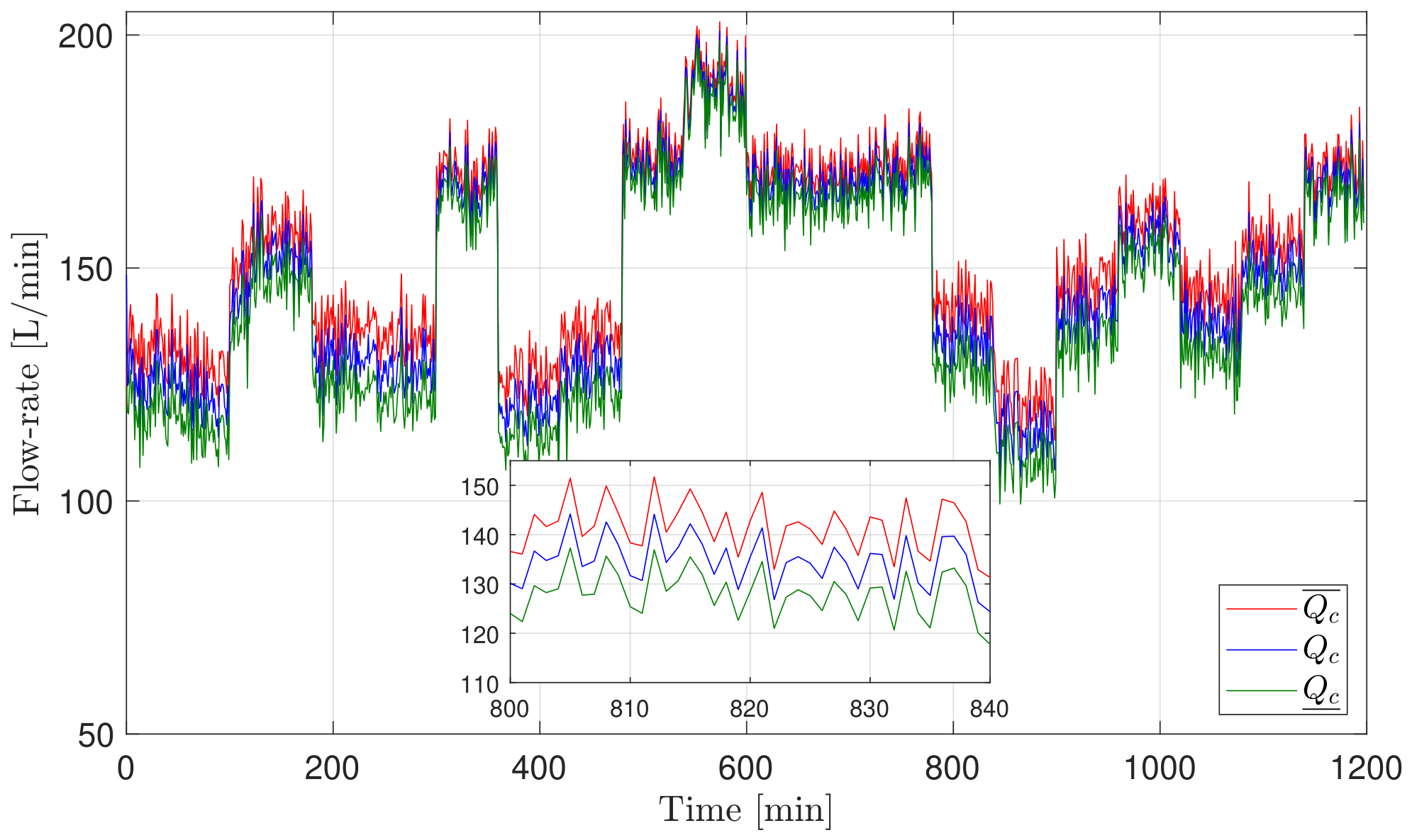
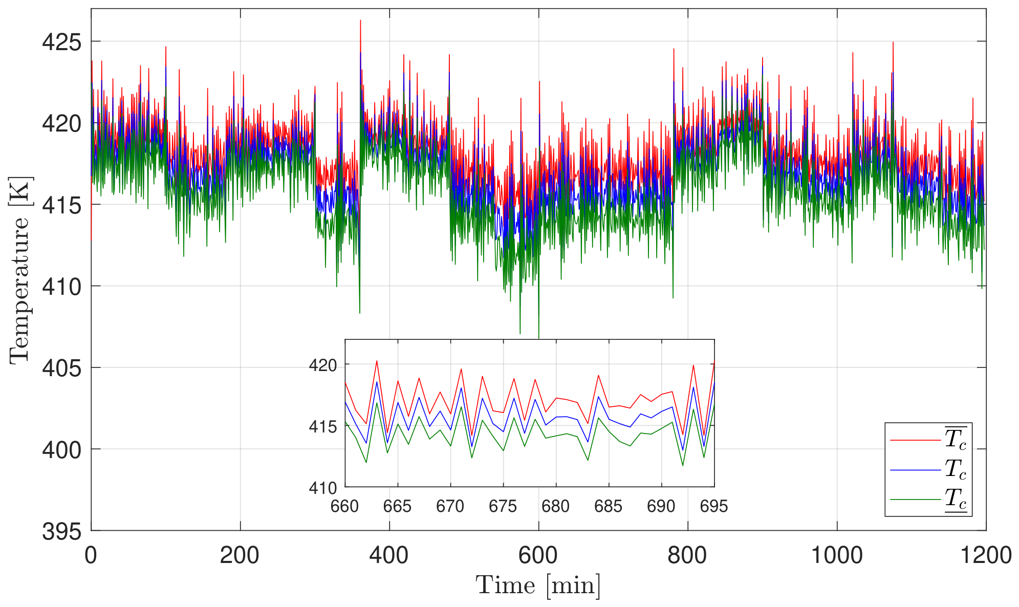
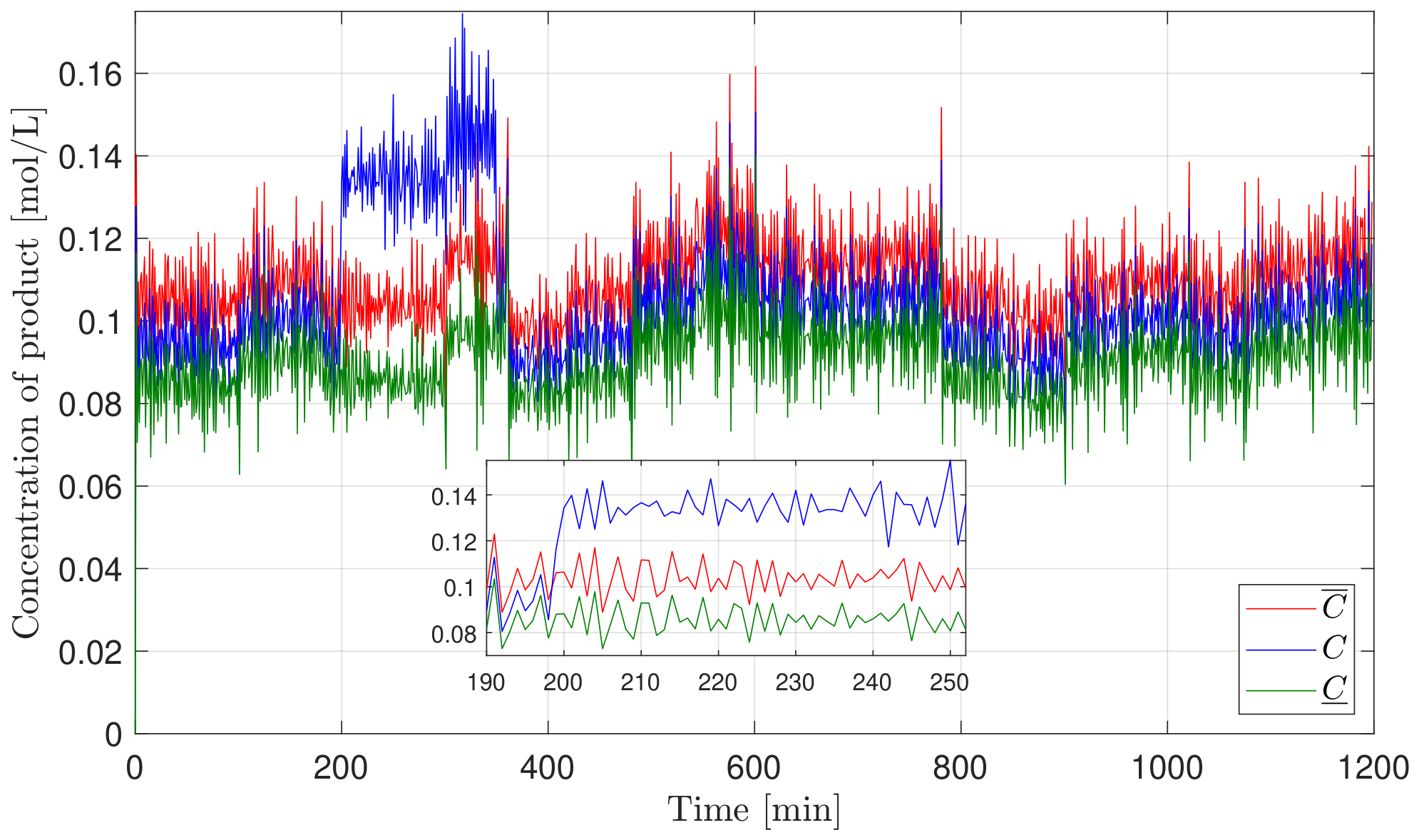
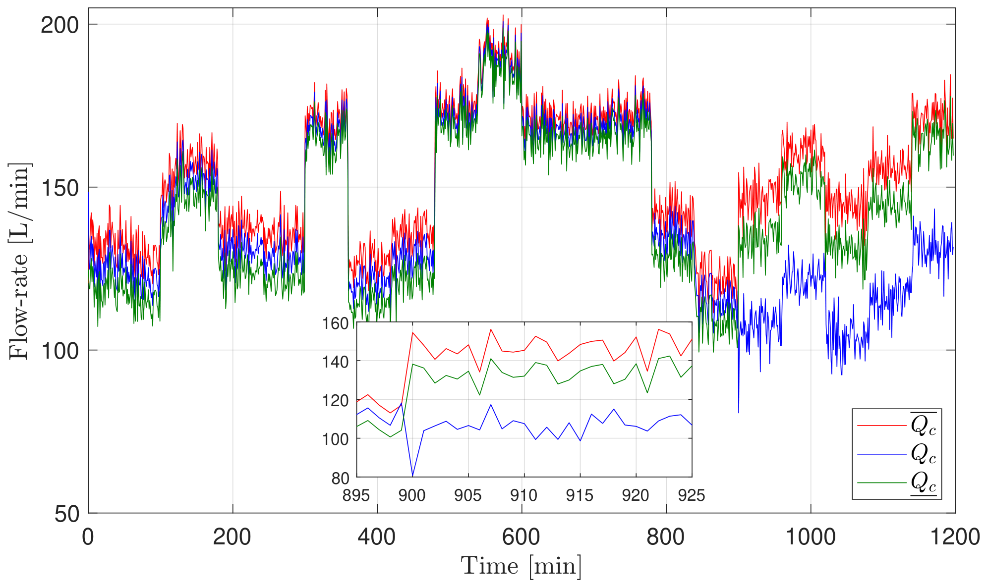
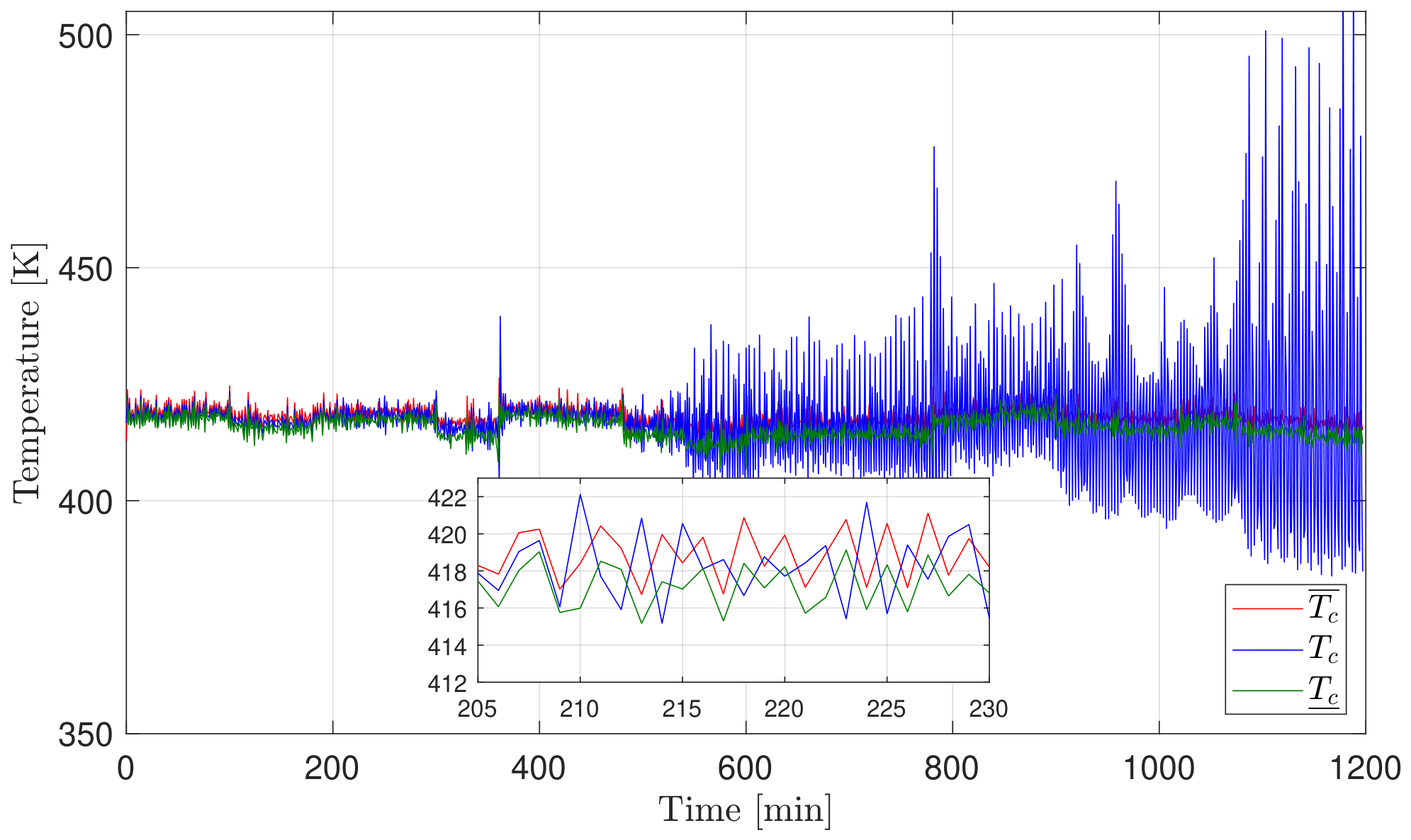
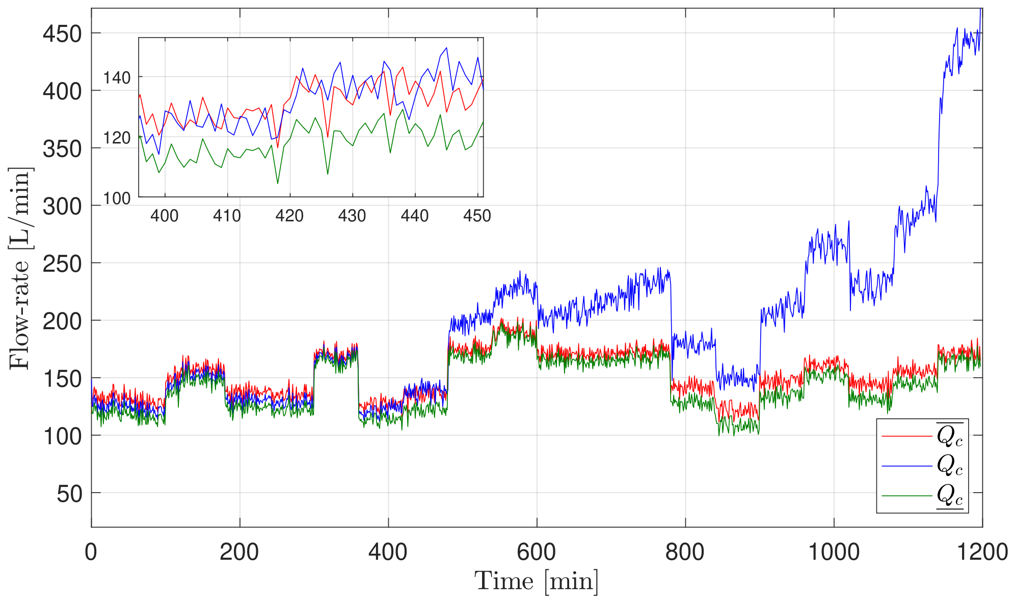
The zonotopic PI observers were subsequently implemented following the methodology detailed in Section 2.4. The resulting estimations are presented graphically to illustrate their behavior under nominal operating conditions. Figure 5 displays the concentration variable C, where the zonotopic bounds (shown in red and green) enclose the measured signal (blue line). Similarly, the temperature T is depicted in Figure 6, while Figure 7 and Figure 8 show the coolant flow rate $Q_c$ and the coolant temperature $T_c$, respectively. In all cases, the observer successfully encloses the measured trajectories, validating its performance under fault-free conditions.

The computational burden of the complete online diagnostic cycle was also evaluated. The measured online execution includes the evaluation of the four ANFIS models, TS model aggregation, zonotopic PI observer update, uncertainty propagation, generator reduction with $q=15$, construction of the measurement-consistent set, intersection testing, and FSM evaluation. The mean computational time was 11.8 ms per sample, with a standard deviation of 2.6 ms and a maximum observed execution time of 24.9 ms.

Considering the sampling interval of $T_s=15$ s, the mean and maximum execution times represent approximately 0.08% and 0.17% of the available sampling period, respectively. ANFIS training and the LMI-based synthesis of the observer gains are performed offline and were therefore excluded from the online timing measurements. These results support the computational feasibility of the proposed implementation for the sampling conditions considered in the CSTR case study.

To evaluate the effectiveness of the proposed method, several tests were performed by intentionally inducing sensor faults and incipient faults in the reactor process. Six fault scenarios were implemented using explicit time-dependent fault profiles. Faults 1–4 correspond to additive sensor faults with linearly varying magnitude over their respective active intervals. Let $t_{f,j}$ and $t_{e,j}$ denote the start and end times of Fault j, respectively, and let ${\delta }_j$ denote the corresponding fault slope. The additive sensor-fault model is defined as

$$y_j^f\left(t\right)=\left\{\begin{array}{cc}{y}_j\left(t\right),\hfill & t<t_{f,j},\hfill \\ y_j\left(t\right)+{\delta }_j(t-t_{f,j}),\hfill & t_{f,j}\le t\le t_{e,j},\hfill \\ y_j\left(t\right),\hfill & t>t_{e,j},\hfill \end{array}\right.$$

(92)

where $y_j\left(t\right)$ denotes the nominal measurement and $y_j^f\left(t\right)$ the faulty measurement. Accordingly, Faults 1–4 are progressive additive faults active only within their prescribed intervals. For the four additive sensor faults considered in this work, the numerical profiles are

$$C^f\left(t\right)=\left\{\begin{array}{cc}C\left(t\right),\hfill & t<200,\hfill \\ C\left(t\right)+0.001(t-200),\hfill & 200\le t\le 350,\hfill \\ C\left(t\right),\hfill & t>350,\hfill \end{array}\right.$$

(93)

$$T^f\left(t\right)=\left\{\begin{array}{cc}T\left(t\right),\hfill & t<350,\hfill \\ T\left(t\right)+0.05(t-350),\hfill & 350\le t\le 600,\hfill \\ T\left(t\right),\hfill & t>600,\hfill \end{array}\right.$$

(94)

$$T_{ci}^f\left(t\right)=\left\{\begin{array}{cc}{T}_{ci}\left(t\right),\hfill & t<600,\hfill \\ T_{ci}\left(t\right)+0.05(t-600),\hfill & 600\le t\le 900,\hfill \\ T_{ci}\left(t\right),\hfill & t>900,\hfill \end{array}\right.$$

(95)

$$Q_c^f\left(t\right)=\left\{\begin{array}{cc}{Q}_c\left(t\right),\hfill & t<900,\hfill \\ Q_c\left(t\right)-0.1(t-900),\hfill & 900\le t\le 1200,\hfill \\ Q_c\left(t\right),\hfill & t>1200.\hfill \end{array}\right.$$

(96)

Fault 5 represents progressive catalyst deactivation. It affects the catalyst activity coefficient a, with nominal value $a_0=1$, and starts at $t_{f,5}=200$ min. Its evolution is modeled as

$$a\left(t\right)=\left\{\begin{array}{cc}{a}_0,\hfill & t<200,\hfill \\ a_0\exp \left[-{\delta }_a(t-200)\right],\hfill & t\ge 200,\hfill \end{array}\right.$$

(97)

with decay rate ${\delta }_a=5\times {10}^{-4}$ min⁻¹. The parameter $a\left(t\right)$ directly scales the reaction-rate term and therefore represents progressive loss of catalyst activity. Fault 6 represents progressive heat-transfer fouling. It affects the heat-transfer efficiency coefficient b, with nominal value $b_0=1$, and starts at $t_{f,6}=400$ min. Its evolution is described by

$$b\left(t\right)=\left\{\begin{array}{cc}{b}_0,\hfill & t<400,\hfill \\ b_0\exp \left[-{\delta }_b(t-400)\right],\hfill & t\ge 400,\hfill \end{array}\right.$$

(98)

where ${\delta }_b=1\times {10}^{-3}$ min⁻¹. As $b\left(t\right)$ scales the heat-transfer contribution, its decrease represents increasing thermal resistance due to fouling. Equivalently, the effective heat-transfer coefficient can be expressed as

$$U{A}_{\mathrm{eff}}\left(t\right)=b\left(t\right)UA.$$

(99)

The numerical configuration of the six evaluated fault scenarios, including the affected variable or parameter, fault onset time, active interval, duration, and fault profile, is summarized in

Table 11. Fault scenarios and numerical profiles used in the CSTR simulations.

Fault	Affected Variable	Start (min)	End (min)	Duration (min)	Profile
1	C sensor	200	350	150	Additive
2	T sensor	350	600	250	Additive
3	$T_{ci}$ sensor	600	900	300	Additive
4	$Q_c$ sensor	900	1200	300	Additive
5	Catalyst activity a	200	1200	1000	Exponential decay
6	Heat-transfer factor b	400	1200	800	Exponential decay

.

Thus, Faults 1–4 are additive sensor faults with finite active intervals and linearly varying magnitude, while Faults 5 and 6 are progressive process faults with exponential decay profiles. In the latter two cases, the affected physical parameters are the catalyst activity coefficient a and the heat-transfer efficiency coefficient b, respectively.

Due to space constraints, only a subset of the fault scenarios is illustrated through selected figures, specifically two sensor faults and two process faults. Figure 9 displays a fault affecting the concentration sensor C, triggered at $t=200\min$, where the measurement exceeds the upper bound of the zonotopic observer. In Figure 10, a fault on the coolant flow-rate sensor $Q_c$ is observed at $t=900\min$, similarly surpassing the upper limit. Figure 11 presents an incipient process fault introduced at $t=200\min$, where the deviation grows progressively and eventually breaches both upper and lower thresholds. Lastly, Figure 12 depicts another incipient process fault, characterized by a gradual increase that results in exceeding the upper zonotopic bound.

Table 12. Activation of residuals for each fault scenario.

Residual	Fault 1	Fault 2	Fault 3	Fault 4	Fault 5	Fault 6
$r_1$	1				1
$r_2$		1			1
$r_3$			1		1	1
$r_4$				1		1

summarizes the residual activation signatures obtained from the dedicated single-fault simulations. Within the six individual fault scenarios considered in this study, all FSM columns are distinct, allowing unique isolation of the evaluated single faults. In particular, Fault 5 activates residuals $r_1$, $r_2$, and $r_3$, while Fault 6 activates $r_3$ and $r_4$.

It should be emphasized that this uniqueness applies to the evaluated single-fault set. Simultaneous faults or residual patterns not represented by the current FSM are classified as ambiguous/unisolated and are not assigned automatically to an existing fault class.

The proposed zonotopic PI observer framework generates adaptive set-based bounds that explicitly account for modeling uncertainty and measurement noise. A fault is detected when the corresponding measured trajectory becomes inconsistent with the predicted zonotopic enclosure. The resulting residual activation patterns are subsequently evaluated through the FSM to isolate the fault scenario. As shown in Table 2, the considered single-fault scenarios produce distinguishable residual signatures, enabling fault isolation under the evaluated conditions. These distinct residual signatures facilitate fault isolation under the considered uncertainty and measurement-noise conditions.

3.2. Performance Under Uncertainty and Measurement Noise

To evaluate the performance of the proposed method under sensor and process faults in the presence of process uncertainty and measurement noise, standard detection metrics are considered as follows:

$$\begin{array}{cc}\hfill \mathrm{Accuracy}& ={\displaystyle \frac{TP+TN}{TP+TN+FP+FN}},\hfill \end{array}$$

(100)

$$\begin{array}{cc}\hfill \mathrm{Recall}& ={\displaystyle \frac{TP}{TP+FN}},\hfill \end{array}$$

(101)

$$\begin{array}{cc}\hfill \mathrm{FPR}& ={\displaystyle \frac{FP}{FP+TN}},\hfill \end{array}$$

(102)

where $TP$, $TN$, $FP$, and $FN$ denote true positives, true negatives, false positives, and false negatives, respectively. Decisions are made sample-by-sample and results are reported per fault and as a macro-average across faults.

For a fair and controlled comparison, three representative data-driven fault-diagnosis approaches were reimplemented following their corresponding methodological formulations: a neural network combined with k-nearest neighbors (NN+kNN) [35], a decision tree induced by genetic programming (DT–GP) [36], and a nonlinear support vector machine with feature selection (SVM–FS) [37].

All comparison methods were evaluated using exactly the same experimental protocol as the proposed approach. Specifically, the same 24 complete fault-free simulations were used for training and the same 6 independent simulations were retained for validation. The methods were supplied with identical CSTR trajectories, sampling conditions, process- and measurement-noise levels and realizations, regressive input structures, and fault profiles. The same fault magnitudes and injection intervals were also maintained throughout the comparative evaluation. Therefore, each method was evaluated sample-by-sample under the same operating, noise, and fault conditions.

The hyperparameters of each baseline method were selected exclusively using the training partition. No samples belonging to the six held-out validation simulations or to the faulty evaluation trajectories were used for hyperparameter selection. Once selected, the resulting configurations were kept fixed throughout the fault-diagnosis experiments.

Table 13. Implementation and training configuration of the comparison methods.

Method	Main Settings	Tuning Strategy	Training Data
NN+kNN	Shallow FFNN (one hidden layer, 5–6 neurons) followed by weighted KNN with Euclidean distance and $k\in [3,10]$	NN size selected according to training error; KNN configuration selected using 5-fold cross-validation	24 simulations (115,200 samples)
DT–GP	Multiclass decision tree induced by genetic programming using tournament selection, crossover, and mutation	Fitness-based evolutionary selection using only the training partition	24 simulations (115,200 samples)
SVM–FS	Nonlinear C-SVM with Gaussian RBF kernel and sensitivity-based feature selection	Grid search for the regularization and RBF-kernel parameters; feature subset selected using the training partition	24 simulations (115,200 samples)
Proposed	64-rule ANFIS–TS model using two membership functions per input and six regressive inputs	Hybrid ANFIS learning for 150 epochs	24 simulations (115,200 samples)

summarizes the implementation and tuning settings employed for all methods.

For all methods, the same six regressive variables associated with each predicted output were generated using the same preprocessing and temporal indices. No baseline method received additional variables, historical samples, or process information. Likewise, the noisy trajectories and fault realizations were generated once and then supplied identically to all methods, thereby ensuring a direct sample-by-sample comparison.

4. Discussion

This discussion synthesizes the quantitative results reported in Section 3, emphasizing the mechanisms that explain the observed performance and the implications for deployment.

The superiority of the proposed scheme stems from the combination of an ANFIS dynamic predictor, capturing dominant nonlinearities and delays, with a zonotopic PI observer that propagates guaranteed state enclosures under bounded uncertainty. The set-inconsistency rule, between measured sets and estimated sets, behaves as an adaptive threshold that widens or tightens with uncertainty, thereby reducing false alarms without sacrificing sensitivity. This mechanism explains the favorable recall–FPR balance observed in

Table 14. ANFIS with zonotopic PI observer (proposed): detection metrics by fault.

Fault	Accuracy (%)	Recall (%)	FPR (%)
1	98.88	99.12	1.93
2	98.47	98.03	2.24
3	98.31	98.58	2.14
4	98.02	98.19	2.47
5	97.83	97.52	2.73
6	98.23	98.01	2.33
Average	98.29	98.24	2.31

,

Table 15. Detection performance obtained with the reimplemented NN+kNN approach following [35].

Fault	Accuracy (%)	Recall (%)	FPR (%)
1	96.83	96.04	3.88
2	96.17	95.07	4.46
3	95.43	94.02	5.23
4	94.91	94.62	5.57
5	94.15	93.47	5.98
6	95.02	94.79	5.41
Average	95.42	94.67	5.09

,

Table 16. Detection performance obtained with the reimplemented DT–GP approach following [36].

Fault	Accuracy (%)	Recall (%)	FPR (%)
1	93.76	92.98	6.82
2	93.23	92.43	7.19
3	92.88	92.11	7.54
4	92.13	91.48	8.12
5	92.02	91.29	8.27
6	93.01	92.04	7.58
Average	92.84	92.06	7.59

and

Table 17. Detection performance obtained with the reimplemented SVM–FS approach following [37].

Fault	Accuracy (%)	Recall (%)	FPR (%)
1	95.62	95.03	4.82
2	95.04	94.08	5.28
3	94.24	93.41	5.93
4	93.73	93.02	6.18
5	93.13	92.24	6.68
6	94.43	93.82	5.71
Average	94.37	93.60	5.77

, especially for sensor-fault cases. In practice, when noise is low the enclosures tighten and enable earlier detections; when uncertainty increases, controlled widening prevents spurious alarms while preserving sensitivity.

When compared with the reimplemented data-driven baseline approaches under the common experimental protocol described above (Table 15, Table 16 and Table 17), the proposed method achieves higher accuracy and lower FPR in both macro-average and per-fault analyses. The advantage is consistent with the use of uncertainty aware, set-based thresholds rather than fixed or purely statistical ones. Differences are most pronounced for sensor faults, where additive shifts create sustained residual separation, and remain favorable for incipient faults despite their slower dynamics.

The diagnostic performance of the proposed framework can be explained by the complementary roles of the ANFIS identification, zonotopic uncertainty propagation, PI observer structure, and $H_{\infty }$ synthesis. The ANFIS stage first provides a nonlinear nominal representation of the CSTR through the weighted combination of local TS submodels. This allows the predictor to adapt to variations within the identified operating region instead of relying on a single fixed linear model.

A second key mechanism is the explicit propagation of identification-induced uncertainty and measurement noise through the zonotopic observer. Consequently, the decision bounds are not fixed a priori. The predicted state enclosure changes according to the current operating condition and the propagated uncertainty. When uncertainty is small, the resulting zonotope remains tighter, preserving sensitivity to deviations from nominal behavior. When uncertainty or measurement noise increases, the enclosure expands accordingly, reducing the probability that admissible nominal variations are incorrectly classified as faults. This mechanism explains the favorable balance between recall and FPR observed in the reported results.

The PI structure provides an additional advantage for persistent deviations. While the proportional correction reacts to the instantaneous output-estimation error, the integral state accumulates persistent discrepancies between measured and estimated outputs. This characteristic is particularly relevant for the incipient process faults considered in this study, whose effects develop gradually and may initially produce relatively small instantaneous residuals. The integral action therefore increases sensitivity to sustained model–process inconsistency without requiring an artificially narrow fixed threshold.

In parallel, the $H_{\infty }$-based synthesis of the observer gains is designed to limit the worst-case influence of bounded process uncertainty and measurement noise on the estimation-error dynamics. The resulting robustness reduces residual variations caused by nonfault disturbances, while the zonotopic consistency test preserves sensitivity when the measured trajectory can no longer be explained by the admissible uncertainty set.

These mechanisms act sequentially and complementarily: ANFIS provides the nonlinear nominal prediction, the zonotopic formulation quantifies admissible uncertainty around this prediction, the $H_{\infty }$ design attenuates the effect of disturbances, and the PI action reinforces the response to persistent deviations. Finally, the FSM exploits the resulting structured residual activation patterns to perform fault isolation. Therefore, the observed diagnostic improvements are associated with the integration of nonlinear identification, uncertainty-aware estimation, robust observer synthesis, and structured residual evaluation rather than with a single component of the framework.

These results also indicate that data quantity should not be considered independently of data representativeness. For the proposed data-driven diagnostic framework, the nominal training measurements should adequately cover the intended operating envelope and provide sufficient excitation of the relevant nonlinear dynamics. Additional samples from an already well-covered operating region provide progressively smaller improvements, while missing operating conditions cannot necessarily be compensated simply by increasing the number of samples. Consequently, representative coverage of the nominal operating region is a fundamental requirement for applying the methodology to experimental or industrial measurements.

4.1. Computational Burden, Scalability, and Online Implementation

The computational requirements of the proposed framework can be separated into offline and online stages. The offline stage comprises ANFIS training, the construction of the uncertain TS representation, and the LMI-based $H_{\infty }$ synthesis of the PI observer gains. These operations are performed once using nominal identification data and are not repeated during online fault monitoring. In particular, the observer gains obtained from the LMI optimization remain fixed during operation.

The complexity of the ANFIS identification stage is strongly related to the number of fuzzy rules. For the adopted structure, the number of rules is $N={\left(N_{\mathrm{MF}}\right)}^{N_{\zeta }}$. As each ANFIS model uses six inputs ($N_{\zeta }=6$) and two membership functions are assigned to each input, the resulting model contains $2^6=64$ fuzzy rules. Increasing the number of membership functions to three or four would increase the rule base to $3^6=729$ and $4^6=4096$ rules, respectively. Consequently, increasing $N_{\mathrm{MF}}$ substantially increases both the number of consequent parameters to be identified and the number of local TS models involved in the subsequent observer formulation. Thus, the two-membership-function configuration provides a parsimonious compromise between nonlinear representation capability and computational tractability.

The LMI-based observer synthesis is also performed offline. Its computational cost increases with the number of local TS models because the stability and robustness conditions are formulated for combinations of local submodels. In the adopted formulation, these pairwise conditions scale quadratically with the number of fuzzy rules, i.e., with $N^2$. Therefore, the computational cost of the synthesis becomes increasingly relevant as the fuzzy rule base grows. However, once feasible observer gains have been obtained, no LMI optimization is required during online operation.

During the online stage, the main operations consist of evaluating and normalizing the fuzzy-rule activation functions, computing the convex aggregation of the corresponding local models, propagating the zonotopic state estimate, constructing the measurement-consistent set, performing the set-intersection test, and evaluating the residual activation pattern through the FSM. The complexity associated with zonotope propagation is controlled by the reduction operator ${\downarrow }_q$. In all simulations, $q=15$ was adopted for a state dimension $n_x=3$, corresponding to a maximum reduced generator budget equal to five times the state dimension. This reduction prevents the continuous growth of the generator matrix during recursive propagation while preserving an outer enclosure of the estimated state set.

Therefore, the proposed implementation places the most computationally demanding identification and optimization procedures in the offline stage, while online diagnosis is carried out using fixed ANFIS parameters, precomputed observer gains, and bounded-order zonotopic propagation. For fixed values of N and q, the online computational burden remains bounded and is mainly associated with low-dimensional matrix and set operations. These characteristics make the proposed framework compatible with online implementation for systems of comparable dimension. Nevertheless, for systems with substantially larger input dimensions, the exponential growth of the fuzzy rule base may become the dominant scalability limitation. In such cases, clustering, rule-pruning, sparse fuzzy representations, or alternative premise-partitioning strategies could be investigated to reduce the number of local models. A dedicated real-time implementation, including hardware-dependent execution-time and memory analyses, remains outside the scope of the present work.

The computational time of the complete online diagnostic cycle was also evaluated over the simulation horizon. The timing includes the four ANFIS model evaluations, convex TS aggregation, PI-observer updates, zonotopic propagation and reduction with $q=15$, measurement-consistent set construction, set-intersection testing, and FSM evaluation. The offline ANFIS training and LMI-based observer synthesis were excluded from the reported online timing.

The experiments were performed in MATLAB (R2025b) on a workstation equipped with a 14th-generation Intel Core i9 processor, 128 GB of RAM, and two 2 TB NVMe solid-state drives. The LMI problems employed during the offline $H_{\infty }$ observer synthesis were formulated using YALMIP and solved with SeDuMi 1.3.

The average online execution time was ${\overline{t}}_{\mathrm{online}}=11.8$ ms per sampling instant, with a standard deviation of 2.6 ms and a maximum observed execution time of 24.9 ms. As the adopted sampling interval is 15 s, the average computational time corresponds to approximately 0.08% of the available sampling period. Even the maximum observed execution time represents only approximately 0.17% of the sampling interval. These results show that the online computational burden is substantially below the available sampling interval, and support the feasibility of online fault monitoring for the considered application and computational platform.

4.2. Applicability to Industrial Measurements

Although the present study is validated using a simulated CSTR benchmark, the proposed methodology is formulated to operate from measured input–output data rather than from an explicit first-principles model. This characteristic facilitates its potential application to industrial processes for which a reliable analytical description is unavailable, incomplete, or difficult to maintain. Nevertheless, transferring the proposed framework to real measurements requires several practical conditions to be considered.

First, the ANFIS identification stage requires a representative set of nominal fault-free data covering the operating region in which the diagnostic system is expected to operate. The available measurements should provide sufficient excitation of the relevant process dynamics, while the sampling rate should be adequate to capture the dominant temporal behavior represented by the regressive structure. Under these conditions, the identification stage can be performed offline using historical process data, and the resulting consequent parameters can be organized into the uncertain TS representation employed by the zonotopic PI observer.

Second, measurement noise and identification uncertainty must be appropriately characterized. In an industrial implementation, measurement-noise bounds can be derived from sensor specifications, calibration information, or the statistical variability observed during nominal operation. Similarly, the uncertainty associated with the identified model can be estimated from the variability of the ANFIS consequent parameters obtained during the identification procedure. These quantities define the uncertainty sets subsequently propagated by the zonotopic observer and therefore directly influence the trade-off between fault sensitivity and robustness against false alarms.

Once the identification stage and observer synthesis have been completed offline, online implementation only requires the evaluation of the ANFIS membership functions, zonotopic state propagation, measurement-consistency testing, and evaluation of the residual activation pattern through the FSM. Thus, no online solution of the identification problem is required during normal monitoring operation.

An important practical limitation is that the reliability of the proposed diagnostic framework depends on the representativeness of the nominal data used for identification. If the process operates substantially outside the identified operating envelope, or if significant model drift, equipment aging, or previously unseen operating modes occur, the identified TS representation may become less accurate. In such situations, the propagated zonotopic sets may become more conservative, potentially increasing detection delay or reducing sensitivity to incipient faults. Periodic model reidentification or an adaptive updating strategy would therefore be required for processes subject to substantial long-term changes.

Accordingly, the results reported in this work should be interpreted as a methodological validation under controlled nonlinear operating conditions rather than as a demonstration of industrial deployment. Validation using experimental platforms and real industrial datasets constitutes a necessary next step to assess long-term model validity, sensor imperfections, process drift, computational requirements, and diagnostic performance under realistic operating conditions.

4.3. Limitations

The ability of the proposed framework to accommodate changing operating conditions depends on whether such conditions remain within the region represented by the nominal identification data. As the TS weighting functions are evaluated online, variations among operating regimes covered by the identified local models are naturally represented through changes in the convex combination of the corresponding submodels. Moreover, identification-induced uncertainty is explicitly incorporated through the matrices ${\mathsf{\Psi }}_i$ and ${\mathsf{\Omega }}_i$ and propagated by the zonotopic observer, providing robustness against bounded deviations from the identified dynamics.

Nevertheless, the local TS parameters and observer gains remain fixed after the offline identification and synthesis stages. Consequently, significant model drift that moves the plant dynamics outside the identified operating region or beyond the uncertainty bounds represented by the model may reduce the accuracy of the state enclosure and degrade fault-diagnosis performance. Under such conditions, the set-membership guarantees established for the identified operating region may no longer be ensured. Addressing long-term model drift would therefore require periodic or adaptive model updating, online reidentification, or multiple TS models covering different operating regimes. These extensions are considered relevant directions for future work.

An additional limitation of the present study is that the fault-isolation scheme is evaluated under a single-fault assumption. The FSM considered in this work is constructed from residual activation patterns associated with individual sensor and process faults. Consequently, unique isolation of simultaneous faults is not guaranteed by the current formulation. In particular, the combined effect of multiple faults may generate an activation pattern that coincides with, or is indistinguishable from, an existing individual-fault signature or another multiple-fault combination, leading to an ambiguous diagnosis. Extension to simultaneous faults would therefore require an augmented FSM containing combined fault signatures and an explicit isolability analysis to verify their distinguishability. Moreover, actuator faults would require the corresponding fault terms to be incorporated into the process/input channel of the identified TS representation and the residual structure to be redesigned accordingly. The diagnosis of simultaneous sensor–actuator faults is therefore left as a direction for future work.

5. Conclusions

This work presents a hybrid fault-diagnosis approach for nonlinear dynamic systems that combines data-driven identification with state estimation via PI-type zonotopic observers. The primary novelty lies in enabling robust fault diagnosis using only measured input–output data, by structuring uncertain TS models through ANFIS and embedding them within a zonotopic ${\mathcal{H}}_{\infty }$ observer framework. The first contribution is the use of an ANFIS model to capture the system’s dominant nonlinearities and delays, yielding a convex TS representation from measured input/output data without requiring additional first-principles information. The second contribution is the design of zonotopic PI observers under an ${\mathcal{H}}_{\infty }$ criterion, which propagate guaranteed state enclosures under bounded uncertainty and generate set-based adaptive thresholds for robust fault detection.

The proposed scheme achieves consistently high detection performance in the CSTR case study. For sensor faults, the method maintains accuracy between 98.02% and 98.88%, indicating early detection with a low false-positive rate despite measurement noise. For incipient process faults, performance is slightly reduced due to smaller residual separation, with accuracy between 97.83% and 98.23%, yet remaining strong overall. On average, the proposed method attains 98.29% accuracy, 98.24% recall, and a 2.31% false-positive rate across all fault types.

Compared with data-driven fault-detection methods reported in the literature, the proposed design achieves higher accuracy and a lower false-positive rate in both macro-average and per-fault analyses. These comparisons were conducted under identical simulation-wise data partitions, process- and measurement-noise conditions, regressive input structures, sampling conditions, and fault profiles, ensuring a fair and reproducible evaluation. These improvements are attributed to the combination of an accurate ANFIS predictor and a zonotopic observer that adapts the decision threshold to prevailing uncertainty via the set-inconsistency test. The framework delivers robust, explainable detection and reliable isolation via a fault-signature matrix, excelling particularly in sensor-fault scenarios while remaining competitive for incipient faults.

The present study also has limitations that define the scope of the reported results. First, the proposed framework has been validated on a simulated CSTR benchmark under single sensor and incipient process faults. Actuator faults and multiple simultaneous-fault scenarios have not been considered; therefore, the current FSM does not guarantee unique isolation when combined faults generate overlapping residual signatures. Extending the framework to these cases will require incorporating actuator-fault effects into the identified TS model, augmenting the residual structure, and performing an explicit isolability analysis for combined fault signatures.

Second, the identified TS representation and observer gains remain fixed after the offline identification and synthesis stages. Consequently, although bounded variations within the identified operating region are explicitly handled by the zonotopic uncertainty representation, significant process drift or operation outside this region may deteriorate the accuracy of the state enclosure and fault-diagnosis performance. Future work will therefore investigate periodic or adaptive model updating to accommodate long-term changes in the process.

Finally, the current results constitute a methodological validation rather than an experimental demonstration of industrial deployment. Future research will extend the proposed framework to experimental platforms and real industrial datasets to assess its performance under realistic sensor characteristics, operating-point variations, process drift, and implementation constraints. Further work will also consider larger-scale nonlinear and cyber-physical systems and the integration of fault-prognosis capabilities for anticipating process degradation with quantified uncertainty.

References

1. Hou, Z.; Lee, C.; Lv, Y.; Keung, K. Fault detection and diagnosis of air brake system: A systematic review. J. Manuf. Syst. 2023, 71, 34–58. [Google Scholar] [CrossRef] [Scilit]
2. Yang, F.; Gao, Z.W.; Lu, S.; Liu, Y. Federated learning for decentralized fault diagnosis of a sucker-rod pumping system with class imbalance data. Control Eng. Pract. 2024, 152, 106050. [Google Scholar] [CrossRef] [Scilit]
3. Fan, S.K.S.; Hsu, C.Y.; Tsai, D.M.; He, F.; Cheng, C.C. Data-driven approach for fault detection and diagnostic in semiconductor manufacturing. IEEE Trans. Autom. Sci. Eng. 2020, 17, 1925–1936. [Google Scholar] [CrossRef] [Scilit]
4. Dakkoune, A.; Vernières-Hassimi, L.; Lefebvre, D.; Estel, L. Early detection and diagnosis of thermal runaway reactions using model-based approaches in batch reactors. Comput. Chem. Eng. 2020, 140, 106908. [Google Scholar] [CrossRef] [Scilit]
5. Jalayer, M.; Orsenigo, C.; Vercellis, C. Fault detection and diagnosis for rotating machinery: A model based on convolutional LSTM, Fast Fourier and continuous wavelet transforms. Comput. Ind. 2021, 125, 103378. [Google Scholar] [CrossRef] [Scilit]
6. Montesuma, E.F.; Mulas, M.; Corona, F.; Mboula, F.M.N. Cross-domain fault diagnosis through optimal transport for a CSTR process. IFAC-PapersOnLine 2022, 55, 946–951. [Google Scholar] [CrossRef] [Scilit]
7. Chen, H.; Li, L.; Shang, C.; Huang, B. Fault detection for nonlinear dynamic systems with consideration of modeling errors: A data-driven approach. IEEE Trans. Cybern. 2022, 53, 4259–4269. [Google Scholar] [CrossRef] [Scilit] [PubMed]
8. Safaeipour, H.; Forouzanfar, M.; Puig, V.; Birgani, P.T. Incipient fault diagnosis and trend prediction in nonlinear closed-loop systems with Gaussian and non-Gaussian noise. Comput. Chem. Eng. 2023, 177, 108348. [Google Scholar] [CrossRef] [Scilit]
9. Chen, Z.; O’Neill, Z.; Wen, J.; Pradhan, O.; Yang, T.; Lu, X.; Lin, G.; Miyata, S.; Lee, S.; Shen, C.; et al. A review of data-driven fault detection and diagnostics for building HVAC systems. Appl. Energy 2023, 339, 121030. [Google Scholar] [CrossRef] [Scilit]
10. Chen, H.; Chai, Z.; Dogru, O.; Jiang, B.; Huang, B. Data-driven designs of fault detection systems via neural network-aided learning. IEEE Trans. Neural Netw. Learn. Syst. 2021, 33, 5694–5705. [Google Scholar] [CrossRef] [Scilit] [PubMed]
11. Peterson, L.; Bremer, J.; Sundmacher, K. Challenges in data-based reactor modeling: A critical analysis of purely data-driven and hybrid models for a CSTR case study. Comput. Chem. Eng. 2024, 184, 108643. [Google Scholar] [CrossRef] [Scilit]
12. Ballesteros-Moncada, H.; Herrera-López, E.J.; Anzurez-Marín, J. Fuzzy model-based observers for fault detection in CSTR. ISA Trans. 2015, 59, 325–333. [Google Scholar] [CrossRef] [Scilit] [PubMed]
13. Bernardi, E.; Adam, E.J. Observer-based fault detection and diagnosis strategy for industrial processes. J. Frankl. Inst. 2020, 357, 10054–10081. [Google Scholar] [CrossRef] [Scilit]
14. Kannan, V.K.; Srimathi, R.; Gomathi, V.; Valarmathi, R.; PrithiEkammai, L. Investigation of unknown input observer for sensor fault diagnosis for a CSTR process. Mater. Today Proc. 2021, 45, 3431–3437. [Google Scholar] [CrossRef] [Scilit]
15. Wilhelm, Y.; Reimann, P.; Gauchel, W.; Mitschang, B. Overview on hybrid approaches to fault detection and diagnosis: Combining data-driven, physics-based and knowledge-based models. Procedia Cirp 2021, 99, 278–283. [Google Scholar] [CrossRef] [Scilit]
16. Abid, A.; Khan, M.T.; Iqbal, J. A review on fault detection and diagnosis techniques: Basics and beyond. Artif. Intell. Rev. 2021, 54, 3639–3664. [Google Scholar] [CrossRef] [Scilit]
17. Venkateswaran, S.; Liu, Q.; Wilhite, B.A.; Kravaris, C. Design of linear residual generators for fault detection and isolation in nonlinear systems. Int. J. Control 2022, 95, 804–820. [Google Scholar] [CrossRef] [Scilit]
18. Bzioui, S.; Channa, R. Estimation and fault diagnosis for non-linear system with time-varying faults and measurement noises: Application on two CSTRs in series. Can. J. Chem. Eng. 2023, 101, 1919–1930. [Google Scholar] [CrossRef] [Scilit]
19. Lan, J.; Patton, R.J. A new strategy for integration of fault estimation within fault-tolerant control. Automatica 2016, 69, 48–59. [Google Scholar] [CrossRef] [Scilit]
20. Boudjellal, M.; Illoul, R. Design of a robust observer with super-twisting algorithm for simultaneous concentration estimation and faults reconstruction in a cstr. Int. J. Chem. React. Eng. 2019, 17, 20180073. [Google Scholar] [CrossRef] [Scilit]
21. Rotondo, D.; Witczak, M.; Puig, V.; Nejjari, F.; Pazera, M. Robust unknown input observer for state and fault estimation in discrete-time Takagi–Sugeno systems. Int. J. Syst. Sci. 2016, 47, 3409–3424. [Google Scholar] [CrossRef] [Scilit]
22. Li, J.; Fang, X.; Zhang, Z.; Wang, Y.; Liu, X.; Zhang, M. Fault detection observer design for Takagi–Sugeno fuzzy systems with finite-frequency specifications. ISA Trans. 2024, 155, 274–285. [Google Scholar] [CrossRef] [Scilit] [PubMed]
23. Zhang, L.; Li, Z.; Li, Y.; Dong, J. State and fault interval estimation for discrete-time Takagi-Sugeno fuzzy systems via intermediate observer base on zonotopic analysis. IEEE Trans. Fuzzy Syst. 2024, 32, 6588–6593. [Google Scholar] [CrossRef] [Scilit]
24. Shafai, B.; Saif, M. Proportional-integral observer in robust control, fault detection, and decentralized control of dynamic systems. In Control and Systems Engineering: A Report on Four Decades of Contributions; Springer International Publishing: Cham, Switzerland, 2015; pp. 13–43. [Google Scholar]
25. Orjuela, R.; Marx, B.; Ragot, J.; Maquin, D. Proportional-Integral observer design for nonlinear uncertain systems modelled by a multiple model approach. In Proceedings of the 2008 47th IEEE Conference on Decision and Control; IEEE: New York, NY, USA, 2008; pp. 3577–3582. [Google Scholar]
26. Le, V.T.H.; Stoica, C.; Alamo, T.; Camacho, E.F.; Dumur, D. Zonotopes: From Guaranteed State-Estimation to Control; John Wiley & Sons: Hoboken, NJ, USA, 2013. [Google Scholar]
27. Combastel, C. A state bounding observer based on zonotopes. In Proceedings of the 2003 European Control Conference (ECC); IEEE: New York, NY, USA, 2003; pp. 2589–2594. [Google Scholar]
28. Combastel, C. A state bounding observer for uncertain non-linear continuous-time systems based on zonotopes. In Proceedings of the 44th IEEE Conference on Decision and Control; IEEE: New York, NY, USA, 2005; pp. 7228–7234. [Google Scholar]
29. Mansouri, M.; Nounou, M.; Nounou, H.; Karim, N. Kernel PCA-based GLRT for nonlinear fault detection of chemical processes. J. Loss Prev. Process Ind. 2016, 40, 334–347. [Google Scholar] [CrossRef] [Scilit]
30. Pilario, K.E.S.; Cao, Y. Canonical variate dissimilarity analysis for process incipient fault detection. IEEE Trans. Ind. Inform. 2018, 14, 5308–5315. [Google Scholar] [CrossRef] [Scilit]
31. Pilario, K.E. Feedback-Controlled CSTR Process for Fault Simulation, Version 1.1.0.1. MATLAB Central File Exchange. 2019. Available online: https://www.mathworks.com/matlabcentral/fileexchange/66189-feedback-controlled-cstr-process-for-fault-simulation (accessed on 25 September 2024).
32. Dong, M.G.; Wang, N. Adaptive network-based fuzzy inference system with leave-one-out cross-validation approach for prediction of surface roughness. Appl. Math. Model. 2011, 35, 1024–1035. [Google Scholar] [CrossRef] [Scilit]
33. Tuan, H.D.; Apkarian, P.; Narikiyo, T.; Yamamoto, Y. Parameterized linear matrix inequality techniques in fuzzy control system design. IEEE Trans. Fuzzy Syst. 2001, 9, 324–332. [Google Scholar] [CrossRef] [Scilit]
34. Chen, J.; Patton, R.J. Robust Model-Based Fault Diagnosis for Dynamic Systems; Springer Science & Business Media: Berlin/Heidelberg, Germany, 2012; Volume 3. [Google Scholar]
35. Naimi, A.; Deng, J.; Shimjith, S.; Arul, A.J. Fault detection and isolation of a pressurized water reactor based on neural network and k-nearest neighbor. IEEE Access 2022, 10, 17113–17121. [Google Scholar] [CrossRef] [Scilit]
36. Rocha, R.C.; Soares, R.A.; Santos, L.I.; Camargos, M.O.; Ekel, P.Y.; Libório, M.P.; dos Santos, A.C.; Vidoli, F.; D’Angelo, M.F. A New Fault Classification Approach Based on Decision Tree Induced by Genetic Programming. Processes 2024, 12, 818. [Google Scholar] [CrossRef] [Scilit]
37. Onel, M.; Kieslich, C.A.; Pistikopoulos, E.N. A nonlinear support vector machine-based feature selection approach for fault detection and diagnosis: Application to the Tennessee Eastman process. AIChE J. 2019, 65, 992–1005. [Google Scholar] [CrossRef] [Scilit] [PubMed]
Figure 1. Scheme of the proposed fault diagnosis method.
Algorithms 19 00689 g001
Figure 2. Diagram illustrating a closed-loop CSTR.
Algorithms 19 00689 g002
Figure 3. ANFIS for CSTR system identification using regressive inputs.
Algorithms 19 00689 g003
Figure 4. Sample dataset of input variables from the CSTR simulation.
Algorithms 19 00689 g004
Figure 5. Concentration C under fault-free conditions.
Algorithms 19 00689 g005
Figure 6. Temperature T under fault-free conditions.
Algorithms 19 00689 g006
Figure 7. Coolant flow-rate Q c under fault-free conditions.
Algorithms 19 00689 g007
Figure 8. Coolant temperature T c under fault-free conditions.
Algorithms 19 00689 g008
Figure 9. Fault 1 in the C sensor at time t = 200 min .
Algorithms 19 00689 g009
Figure 10. Fault 4 in the Q c sensor at time t = 900 min .
Algorithms 19 00689 g010
Figure 11. Fault 5 in the reactor process at time t = 200 min .
Algorithms 19 00689 g011
Figure 12. Fault 6 in the reactor process at time t = 400 min .
Algorithms 19 00689 g012