Thermal Performance Prediction of Satellite Battery Using Machine Learning: A Case Study

Abstract

Satellite battery subsystems are fundamental for reliable operation during periods when solar power is unavailable. Their performance is strongly influenced by the harsh and variable thermal conditions of the space environment. Pre-launch thermal simulations are routinely employed to evaluate subsystem behaviour; however, their ability to fully represent in-orbit dynamics remains limited. Meanwhile, machine learning (ML) approaches have emerged for satellite health monitoring, yet their practical role alongside conventional thermal analysis is not clearly established. This study investigates satellite battery temperature prediction by integrating pre-launch thermal simulation, real in-orbit telemetry, and data-driven ML forecasting within a unified framework. A dataset of 27,552 temperature measurements from an operational low-Earth-orbit satellite was analysed. A sliding-window regression approach was used to predict one-hour-ahead minimum and maximum battery temperatures, consistent with operational thermal margins. Three models—linear regression, Random Forest, and Extreme Gradient Boosting—were trained using historical temperature data and evaluated against telemetry and simulation outputs using MAE, RMSE, and R² metrics. Results indicate that linear regression achieved the highest accuracy (R² up to 0.98, MAE ≈ 0.20 °C), outperforming more complex models. ML-based predictions captured thermal behaviour more effectively than static simulation outputs under nominal conditions, while all predicted values remained within the acceptable operational range (10–30 °C). Rather than replacing physics-based methods, this work demonstrates that interpretable ML models can serve as an effective real-time complement to thermal simulations, offering practical insights into model selection and enhancing satellite battery thermal monitoring.

1. Introduction

Satellite battery subsystems are fundamental for reliable spacecraft operation during eclipse periods when solar power is unavailable and the satellite relies entirely on stored battery energy. Under these conditions, battery temperature directly affects the electrochemical efficiency, available capacity, internal resistance, degradation rate, cycle life, and overall operational reliability. Excessively high temperatures accelerate battery degradation and ageing, whereas low temperatures reduce available power and charging efficiency. Consequently, maintaining battery temperature within its specified operational limits is essential for ensuring mission safety, extending battery lifetime, and guaranteeing uninterrupted spacecraft operation. Therefore, it is subject to strict acceptance limits throughout satellite missions. To ensure compliance with these limits, battery thermal behaviour is traditionally assessed during the design phase using numerical thermal simulations, which account for orbital environment, spacecraft configuration, and thermal control mechanisms. However, such simulations are inherently limited by modelling assumptions, parameter uncertainties, and their static nature once the satellite enters operation [1,2], motivating interest in complementary data-driven approaches during mission execution.

The application of ML in spacecraft is a growing area of research [3,4]. As the deployment of satellites such as CubeSats and small satellites continues to rise, ML has the potential to improve accuracy and robustness by enabling self-monitoring, self-diagnosis, and real-time corrections. It can process large amounts of data by identifying patterns and trends that may not be evident through traditional thermal simulation modelling. The integration of ML with traditional methods serves as a powerful tool for improving the prediction of satellite subsystem performance. Implementing this integrated approach to satellite battery performance can extend battery lifetime, thereby improving the overall reliability of satellite missions. Furthermore, it can enhance the decision-making capabilities of mission operators and onboard systems by reducing overly conservative operational margins.

Satellite batteries are vital for operation, particularly when solar energy is unavailable. Reliable batteries are essential for satellites to transmit data and manage functions. However, the harsh environment of space poses challenges to battery performance. Radiation and extreme temperatures can reduce battery efficiency. Therefore, it is important to select a suitable energy capacity for each satellite mission. The type of battery used in a satellite can vary depending on the satellite’s size. Several factors are considered when choosing batteries, including peak power requirements, worst-case orbit energy requirements, operating temperature, and mission duration [5,6].

Numerous previous studies have applied ML in the realm of satellite battery subsystems. Ahmad et al. [7] proposed that the combination of ML with a statistical survival method was applied for health monitoring of satellite batteries. This approach combined ML pattern recognition with logical analysis of data (LAD) and Kaplan–Meier (KM) estimator survival analysis. It demonstrated significant improvements in predicting the remaining useful life of satellite batteries compared to using KM alone. De Canio et al. [8] developed a Random Forest model to predict spacecraft thermal behaviour from training data from previous eclipse telemetry recordings and predict the temperature of six key instruments. The objective of this model was to predict the thermal behaviour of these instruments to enable smarter heater scheduling, optimise battery usage, and increase the lifetime of operational spacecraft. Donato [9] investigated the internal impedance of lithium-ion battery packs in the satellite system. Two supervised learning models, namely XGBoost and a multi-layer perceptron neural network, were developed, with results indicating that the models could accurately estimate the internal impedance of satellite batteries using telemetry data. This method provided a practical route for real-time health monitoring of satellite batteries, effectively overcoming the limitations of traditional electrochemical impedance spectroscopy. Research on satellite batteries and attitude determination and control systems was conducted in [10,11], comparing real data obtained from the satellite ground station during operation with results from thermal tests conducted prior to launch. The results showed that the real data aligned with the thermal test results within the acceptable temperature range. While ML has shown promising results in predicting battery performance, its implementation in satellite battery systems necessitates further research to validate its advantages [12]. The monitoring of satellite battery logs generates large time-series datasets, which are well-suited for training ML models. However, prediction accuracy is heavily influenced by the choice of an appropriate model that aligns with the study’s objectives, available parameters, data quality, and computational constraints.

A key objective of this research is to evaluate the efficacy of regression techniques, a subset of supervised learning, particularly in predicting satellite battery temperatures un-der varying orbital conditions. Regression is well-suited for forecasting continuous numerical values. This study compares the performance of a basic regression model, linear regression, known for its simplicity and interpretability, with more advanced ensemble methods, specifically Random Forest and Gradient Boosting, which can model complex, nonlinear relationships to improve prediction accuracy.

Despite the growing interest in applying machine learning techniques to satellite battery monitoring, there remains a lack of systematic studies that integrate data-driven forecasting with traditional thermal analysis in a manner that is both physically interpretable and operationally relevant. In particular, it is still unclear under what conditions machine learning models can meaningfully supplement pre-launch thermal simulations. Additionally, questions persist regarding how model complexity should be selected for orbit-driven thermal systems. Furthermore, existing studies often evaluate machine learning predictions independently, without quantitatively benchmarking them against both simulation results and real in-orbit telemetry within a unified framework.

Motivated by these gaps, this study presents an investigation into satellite battery temperature prediction that explicitly integrates pre-launch thermal simulation, real ground-station measurements, and machine learning-based forecasting. The work focuses on identifying the appropriate model complexity, physical interpretability, and operational value for thermal prediction under nominal orbital conditions. By employing a sliding-window regression strategy and evaluating prediction bounds aligned with thermal acceptance limits, the study provides valuable insights into when simple data-driven models can outperform more complex approaches. It also illustrates how machine learning can serve as a practical complement rather than a replacement for thermal simulations.

Unlike previous studies that focus exclusively on either thermal simulation or machine learning, this work integrates pre-launch thermal simulation, in-orbit telemetry, and machine learning prediction within a unified framework for satellite battery thermal assessment. Furthermore, the study systematically compares simple and ensemble regression models under identical operating conditions and demonstrates that an interpretable linear regression model can outperform more complex learning algorithms for short-term thermal prediction. These findings provide practical guidance for selecting machine learning models suitable for operational spacecraft thermal monitoring. The paper is structured into different sections. The first section is the introduction. The second section presents the numerical analysis used in this study, including the thermal model, numerical method, and thermal test. The ML methods applied in this work are outlined in the third section. The results derived from both thermal analysis and machine learning are discussed in the fourth section. Finally, the manuscript concludes with a summary and outlines the future research directions in Section 5.

2. Satellite Thermal Analysis Approach

2.1. Satellite Structure and Thermal Model

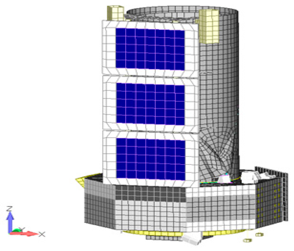
The design and structure of a satellite are essential for effective operation, reliability, and survival in the challenging conditions of the space environment. Throughout their lifespan, satellite subsystems must endure various physical and environmental stresses, including the intense mechanical loads experienced during launch, prolonged exposure to high solar flux, temperature fluctuations, and potential collisions with micro-debris in orbit. To fulfil mission objectives, the satellite structure is designed as a 3D model. This model provides detailed information about the geometry and configuration of satellite components, enabling the application of finite element methods for evaluating structural and thermal behaviour. As illustrated in Figure 1, the thermal model of the satellite was created using FEMAP software version 11.3 [13] as the analytical solver. The thermal model is employed to characterise the temperature distribution across satellite subsystems, serving as an essential tool for accurate temperature prediction and control under anticipated space conditions.

Figure 1. 3D thermal modelling of satellites.

2.2. Mathematical Modelling and Governing Equation

All satellite components are required to maintain specific temperature ranges to ensure their survival and effective operation throughout all mission phases. A satellite’s temperature is influenced by the amount of heat it absorbs, generates, stores, and dissipates. In orbit, satellites are subjected to extreme thermal variations, ranging from very cold to very hot conditions. In the space environment, heat transfer primarily occurs through conduction within the satellite and radiation from its surfaces. The fundamental equation used in satellite thermal analysis is the energy balance equation. This equation is critical for understanding how heat is exchanged between the satellite and its environment. For a satellite in space, the energy balance equation is used to describe the balance between the energy absorbed from external sources (mainly the Sun and Earth) and the energy emitted by the satellite as thermal radiation, and it can be expressed as:

$$Q_{stored}=Q_{in}-Q_{out}$$

(1)

$$m{C}_p{\displaystyle \frac{dT}{dt}}=Q_{in}-Q_{out}$$

(2)

The energy balance Equation (1) incorporates transient, conduction, and radiation terms. The individual terms are expanded in more detail, where Q_stored (W) is the rate of heat stored by the satellite and is determined by the satellite’s thermal capacitance. Q_in (W) is the total heat input to the satellite, including incident solar radiation, solar albedo, Earth infrared (IR) radiation, and internally generated heat from onboard equipment. Finally, Q_out (W) is the total heat rejected by the satellite through thermal radiation, as described in the following equations. Furthermore, m is the satellite mass (kg), and Cp is the specific heat capacity (J/kg·K). The rate of change in temperature with time is represented by dT/dt (K/s). Now, before expanding the heat input Q_in and the heat rejected Q_out in Equation (2), all terms representing the heat input to the satellite and the heat output from the satellite will be defined. The total heat input to the satellite includes incident solar radiation, solar albedo, Earth infrared radiation and heat generation. The incident solar radiation is the direct electromagnetic radiation emitted by the Sun and absorbed by the satellite’s external surfaces. It is typically the largest external heat source when the satellite is illuminated. Solar albedo radiation is the portion of solar radiation reflected by the Earth’s surface and atmosphere that reaches and is absorbed by the satellite. Its magnitude depends on the Earth’s reflectivity (albedo), the satellite’s position, and the viewing geometry. Earth infrared (IR) radiation is the thermal infrared radiation naturally emitted by the Earth due to its temperature. This radiation provides a continuous external heat input, including when the satellite is in eclipse, provided the Earth remains within the satellite’s field of view. Finally, the internal heat generation is the heat produced within the satellite by onboard components and subsystems, such as electronic circuits, batteries, communication equipment, sensors, and payload instruments, as they consume electrical power. The heat input to the satellite can be expressed as:

$$Q_{in}=Q_{solar}+Q_{Albedo}+Q_{IR}+Q_{gen }$$

(3)

$${ Q}_{Out}=Q_{radiated }$$

(4)

where Q_solar (W) is the incident solar radiation, Q_albedo (W) is the reflected solar radiation (albedo), Q_IR (W) is the Earth-emitted infrared radiation, and Q_gen (W) is the internal heat generation.

Now, Equation (2) can be rewritten by expanding each term:

$$m{C}_p{\displaystyle \frac{dT}{dt}}=Q_{solar}+Q_{Albedo}+Q_{IR}+Q_{gen}-Q_{out}$$

(5)

Now, Equation (5) can be further expanded as:

$$Q_{solar}=\alpha A q_s \cos \theta$$

(6)

$$Q_{Albedo}=\alpha A q_s A_{alb} F_{Earth-satellite}$$

(7)

$$Q_{IR}=\epsilon A q_{earth} F_{Earth-Satellite}$$

(8)

$$Q_{out}=\epsilon \sigma A \left(T_1^4-T_2^4\right) F_{1-2}$$

(9)

where α is the absorptivity, ε is the emissivity, σ is the Stefan–Boltzmann constant (5.67 × 10⁻⁸ W/m²K⁴), A is the surface area in m², q_s is the solar constant in W m⁻², θ is the incident angle between the solar normal vector and the solar vector in degrees, A_alb is the albedo factor, q_earth is the Earth’s infrared radiation in W m⁻², with F_{Earth-satellite} being the view factor between the Earth and the satellite surface, and F₁₋₂ is the view factor between the satellite and space. In Equation (9), T₁ and T₂ represent the satellite component temperature and the space temperature, respectively, in Kelvin K. All variables are expressed using SI units, while the absorptivity (α), emissivity (ε), albedo factor (A_alb), and view factors are dimensionless. In this study, the entire satellite system was solved and analysed; therefore, the values of the thermophysical and optical properties are related to the satellite battery component, as presented in Table 1 [14,15].

Table 1. Satellite battery thermophysical and optical properties.

Property	Value
Absorptivity	0.2
Emissivity	0.03
Density	2700 kg/m3
Specific Heat	940 J/kg·K
Thermal Conductivity	167 W/m·K

In the numerical simulation analysis, boundary and operating conditions are essential for solving the equations presented above for the entire system. The FEMAP software solves the thermal energy balance equation under transient conditions by using orbital parameters and thermophysical and optical properties, along with boundary conditions such as solar fluxes and temperature. Table 1 presents the thermophysical and optical properties of the battery. The temperature of space is 4 K, while the temperature of the Earth is 257 K. The view factor between the Earth and the satellite surface (F_{Earth-satellite}) is 0.3, and the view factor between the satellite and space (F₁₋₂) is 1 [15]. The remaining thermal boundary conditions will be shown in subsequent tables in Section 2.3.

2.3. Numerical Method and Model Analysis Cases

The numerical simulation of a satellite entails resolving the computational model to study the thermal characteristics and dynamic behaviour of satellites operating within the space environment. This study specifically targets one critical satellite subsystem: the satellite batteries. Utilising FEMAP software [13] and finite element analysis, the satellite thermal model is solved. The results compare the temperature profiles of the batteries across three distinct scenarios: the nominal case, the hot case, and the cold case. The hot and cold cases represent potential worst-case thermal environments, with the hot case corresponding to maximum solar radiation and, consequently, the highest heat fluxes, while the cold case corresponds to minimum solar heat fluxes. The nominal case employs average solar heat flux values to reflect typical operational conditions. To accurately capture significant power fluctuations impacting the satellite batteries, the simulations are conducted over the duration of a single solar day. The analysis cases of this study are presented in Table 2. From Table 2, the nominal, hot, and cold cases follow the standard spacecraft thermal design methodology [15] used during mission analysis. The hot case represents the worst-case solar heating condition associated with the December solstice, whereas the cold case corresponds to the lowest expected external thermal loading during the June solstice. The nominal case represents average orbital environmental conditions for the thermal analysis (the arithmetic mean of the corresponding hot- and cold-case values). The adopted values of solar flux, Earth albedo, and Earth infrared radiation were selected according to standard spacecraft thermal analysis practice and published thermal environment data.

Table 2. All thermal analysis cases [15,16].

Parameter	Nominal Case	Hot Case	Cold Case
Time of Year	Mean of the hot- and cold-case values	December Solstice	June Solstice
Solar Flux	1368.6 W/m2	1411.6 W/m2	1323.6 W/m2
Albedo	0.306	0.35	0.24
Earth IR	237 W/m2	263 W/m2	224 W/m2
Internal Dissipation	Full Performance	Full Performance	Housekeeping
Thermo-optical Properties	Beginning of Life	End of Life	Beginning of Life

A mission-representative orbit, as described in Table 3, is used for the analysis.

Table 3. Orbit definition [16].

Parameter	Value
Type	Sun-synchronous
Altitude	547 km
Eccentricity	0 (-).
Orbit inclination	97.63 deg.
Orientation	Primary: −Y aimed at Sun Secondary: +Z aligned with Nadir

2.4. Thermal Test

The thermal testing of satellite components is a crucial part of the testing process during satellite development. Satellite power systems rely on high-performance batteries, which must operate under extreme conditions, including radiation, vacuum, and temperature fluctuations. Post-manufacturing testing verifies battery integrity, capacity, safety, and reliability before their integration into the satellite system. Since satellites operate in the harsh conditions of space, where temperatures can vary dramatically, testing the thermal performance of satellite components is imperative to ensure they can withstand extreme temperature fluctuations, maintain the temperatures of satellite components within their operational range, and remain operational throughout the mission. The temperatures of the satellite batteries were measured [14] to ensure compatibility with the space environment, confirming that their values fall within the range of 10 to 30 °C.

Unlike automotive or stationary battery systems, satellite batteries operate under unique environmental conditions characterised by vacuum, cyclic solar illumination, eclipse transitions, radiation exposure, and limited maintenance opportunities after launch. Consequently, satellite battery temperature prediction is primarily governed by orbital dynamics, spacecraft thermal design, and mission operating conditions rather than ambient environmental variations. These characteristics make satellite thermal prediction a distinct and more constrained forecasting problem.

3. Machine Learning Approach

3.1. Dataset Description

The dataset used in this study comprises 27,552 in-orbit temperature measurements from a single battery aboard the satellite. Telemetry data were collected via the ground station operated by the King Abdulaziz City for Science and Technology (KACST) [16]. Each entry includes a Coordinated Universal Time (UTC) timestamp recorded at five-minute intervals, along with the corresponding battery temperature in degrees Celsius.

Data collection spans from 2019 to 2022, with discontinuous temporal coverage. The monthly data availability varies, with record counts ranging from 861 to 4592 per month, which is equivalent to approximately three to 16 days of observations.

The data were processed to address any irregular sampling issues by selecting only continuous sequences without gaps exceeding six minutes and constructing sliding-window sequences that incorporate the preceding hour of temperature measurements for each timestamp.

3.2. Data Preprocessing

The telemetry dataset comprised timestamped temperature readings derived from the satellite’s battery logs, which were initially sorted to preserve temporal order. The first step involved sorting the data chronologically to maintain temporal integrity. Readings that fell outside the operational range of –10 °C to 50 °C were treated as anomalies and subsequently removed. It is crucial to ensure a consistent temporal structure for time-series modelling, particularly in predicting short-term thermal patterns. Given a logging interval of five minutes, a complete 24 h period should yield 288 measurements. The dataset underwent daily evaluation, and any days with more than 70% missing data from 201 entries were excluded from the analysis to prevent unreliable interpolation and guarantee data reliability.

For the remaining days, missing values were addressed using a combination of linear interpolation and directional filling. Linear interpolation estimates values based on their adjacent known data points. Let $\widehat{{\chi }_t}$ denote the temperature at the missing time step t, and let ${\chi }_{t1}$ and ${\chi }_{t2}$ represent the known temperature values immediately before and after the missing point, respectively. The interpolated value was computed using Equation (10).

$$\widehat{{\chi }_t}={\chi }_{t1}+{\displaystyle \frac{{\chi }_{t2}-{\chi }_{t1}}{t_2-t_1}} . (t-t_1)$$

(10)

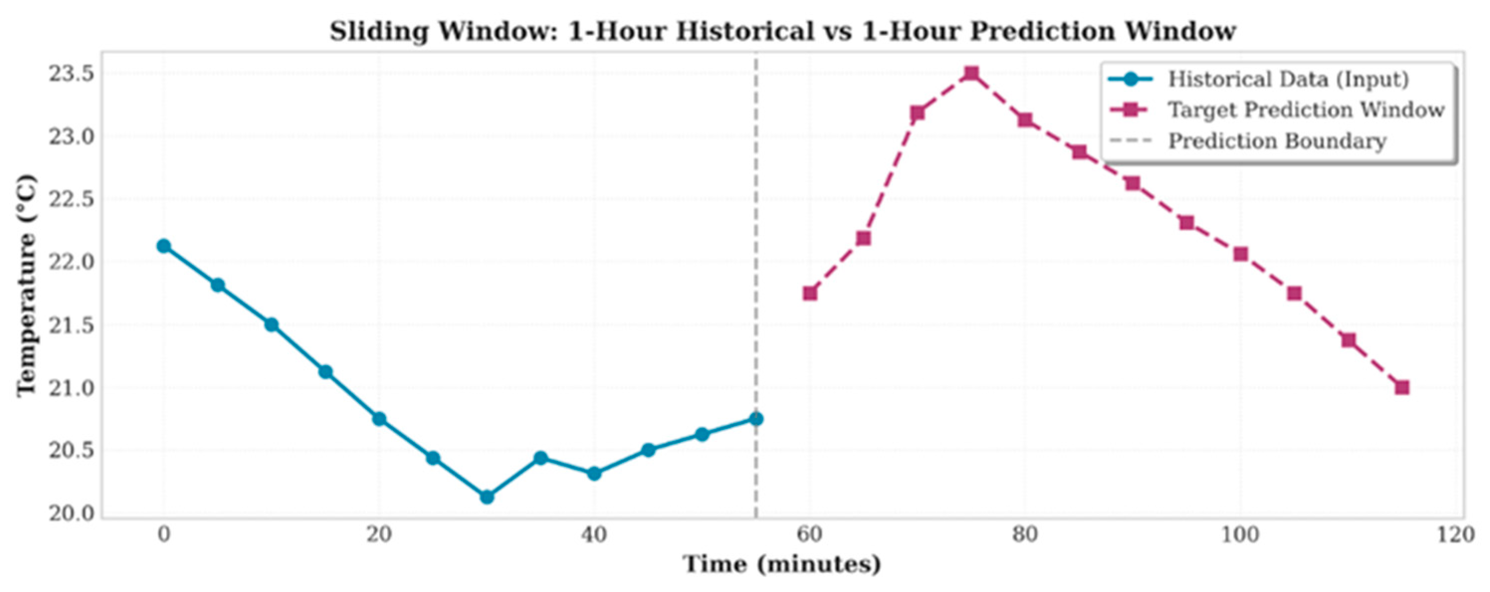
To prepare the dataset for supervised learning, a sliding-window strategy was implemented. This approach used a window of 12 steps, equal to one hour, given the five-minute sampling interval, to extract past temperature readings as model input and the next 12 steps as the prediction target. Only sequences without gaps exceeding six minutes within either the past or future segments were retained to ensure temporal continuity and preserve meaningful patterns for learning. Each input and output pair was constrained to remain within the same calendar day to avoid inter-day variability, although sequences occurring in the final hour of the day were still included if they satisfied the continuity criteria. An example of this sampling strategy is depicted in Figure 2, where the first 12 points represent the input and the following 12 points represent the target output.

Figure 2. Example of a sliding-window sample with twelve input values from the past hour and twelve target values for the next hour.

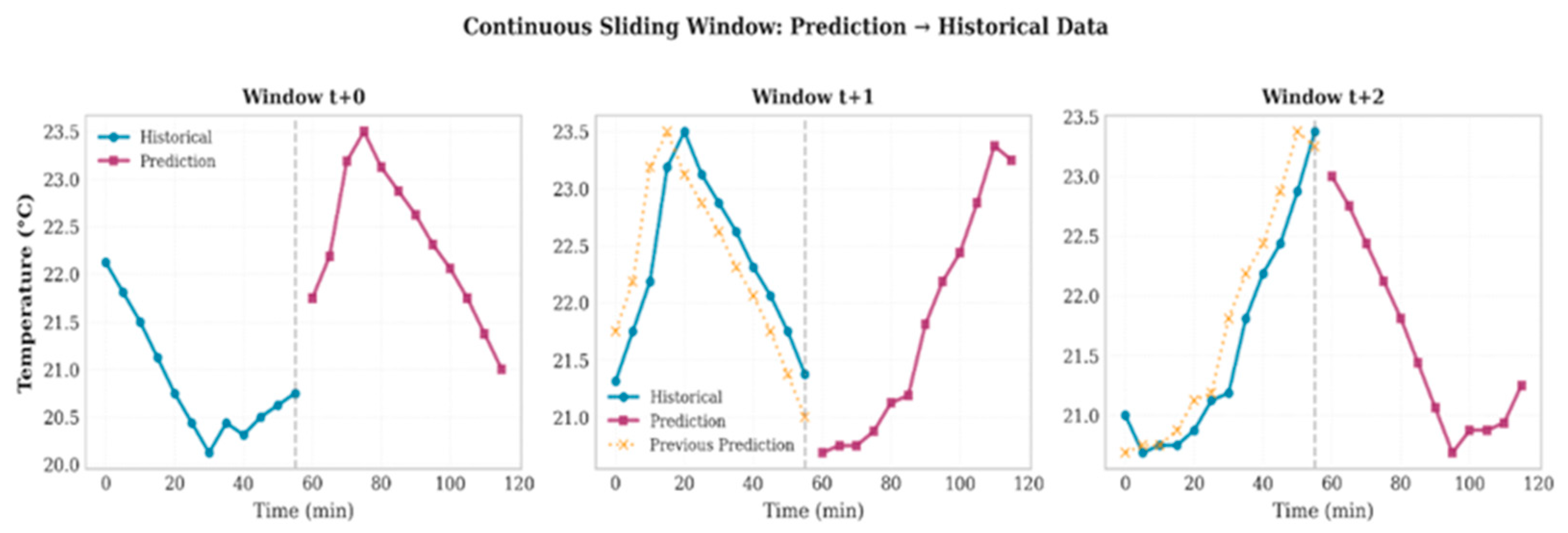
To further demonstrate the inherent continuity of this method, Figure 3 presents three consecutive sliding windows extracted from a continuous time sequence. This visualisation highlights a key principle of the approach: the prediction target from window t becomes part of the historical input for window t + 1. This overlapping structure allows the model to learn from a continuously evolving data stream, rather than disjointed sequences, thereby capturing the short-term dependencies that are critical for high-resolution forecasting.

Figure 3. Three consecutive sliding windows showing temporal continuity. The prediction target of window t becomes the historical input for window t + 1.

Finally, the resulting data samples were chronologically divided into training and testing sets, with the initial 70% allocated for training and the remaining 30% reserved for evaluation, thereby preserving the natural time sequence. Hyperparameter optimisation was conducted exclusively on the training set using grid search with three-fold time-series cross-validation (Time-Series Split), which preserves temporal order within each fold, while the test set was reserved solely for final performance evaluation.

3.2.1. Linear Regression

Linear regression was employed as a baseline model to assess the suitability of simple, interpretable relationships for short-term satellite battery temperature prediction. The model was formulated to map historical battery temperature sequences to one-hour-ahead minimum and maximum temperature values using an ordinary least squares approach. Given the relatively narrow operating temperature range and the smooth, orbit-driven thermal dynamics of the battery system, linear regression provides a useful reference for evaluating whether increased model complexity is justified.

The input features consisted of sliding-window segments of recent temperature measurements, while the outputs corresponded to the minimum and maximum battery temperatures within the subsequent prediction horizon. No regularisation was applied, as preliminary analysis indicated stable model behaviour and no evidence of multicollinearity or overfitting. Model training was performed using the designated training dataset, and predictions were generated without iterative updates during the test phase to emulate real-time operational forecasting conditions.

3.2.2. Random Forest

Random Forest regression was implemented to evaluate the performance of an ensemble-based, nonlinear learning approach for capturing potential deviations from linear thermal behaviour. The model was configured as a multi-output regressor to simultaneously predict the minimum and maximum battery temperatures within the one-hour forecasting horizon.

Key hyperparameters, including the number of decision trees, maximum tree depth, and minimum samples per split, were optimised through grid search using the training dataset. Bootstrap sampling was enabled to improve robustness, while feature importance analysis was not explicitly utilised, as the primary objective was predictive performance rather than model interpretability. The Random Forest model was trained exclusively on historical temperature sequences, consistent with the operational forecasting scope of the study.

3.2.3. Extreme Gradient Boosting

Extreme Gradient Boosting (XGBoost) was adopted as a representative gradient-boosted ensemble method to assess whether incremental, sequential learning could improve short-term prediction accuracy for satellite battery temperature extremes. Similar to the Random Forest implementation, the XGBoost model was configured for multi-output regression to predict one-hour-ahead minimum and maximum temperature values.

Hyperparameters governing tree depth, learning rate, and the number of boosting iterations were tuned via grid search on the training dataset to balance model capacity and generalisation. Early stopping criteria were applied during training to mitigate overfitting. The model utilised only historical battery temperature measurements as inputs, in line with the study’s focus on short-term, data-driven forecasting under nominal operating conditions.

3.3. Model Architecture

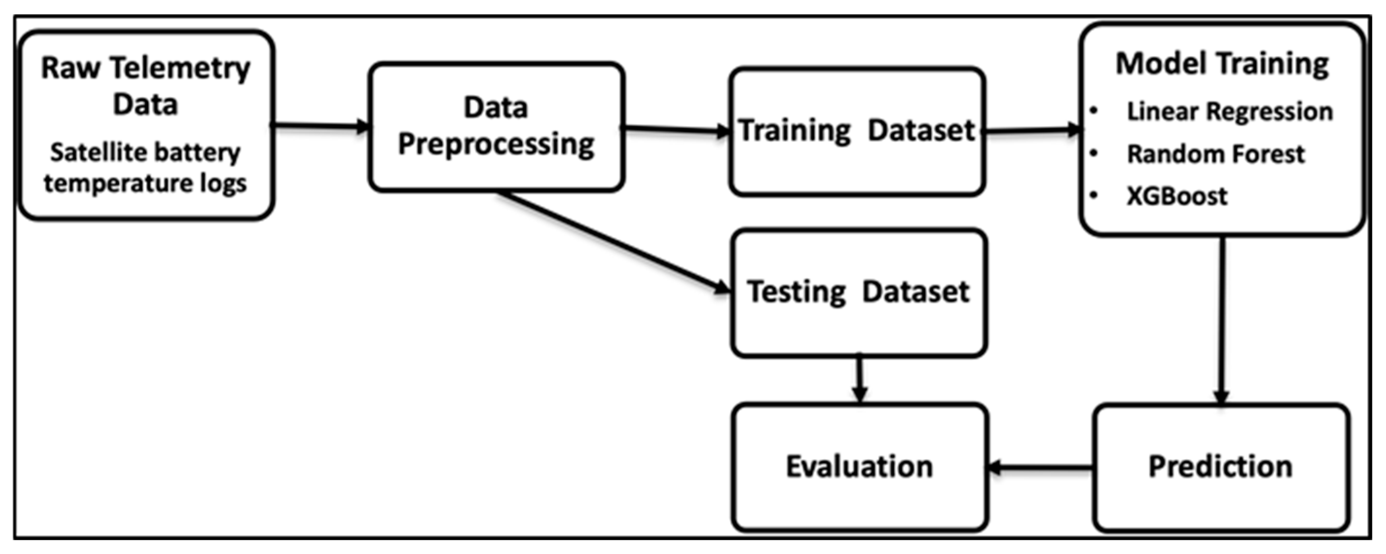
The overall model workflow is illustrated in Figure 4, encompassing data preprocessing, sliding-window generation, dataset splitting, model training, prediction, and performance evaluation. Each model—linear regression, Random Forest, and XGBoost—was trained independently, followed by a comparative analysis of their forecasting accuracy.

Figure 4. The model workflow.

Temporal dependencies were captured using a fixed-length sliding-window approach. Each input sample consisted of 12 consecutive temperature measurements from the preceding hour, allowing the models to learn temporal patterns without the need for manual lag feature engineering. This approach embeds temporal information directly into the input, rendering it appropriate for tree-based models such as Random Forest and XGBoost.

For the ensemble models, hyperparameter tuning was performed using grid search. The grid search aimed to minimise the mean absolute error (MAE) on the validation set. The parameter values searched for each model are summarised in Table 4.

Table 4. Parameters for Random Forest and XGBoost.

Parameter	Random Forest	XGBoost
n_estimators	50, 100, 200, 300	100, 200, 300, 500
max_depth	2, 3, 5, 10, 15, 20, 30	2, 3, 5, 7
learning_rate	-	0.01, 0.1

The optimal configuration for the Random Forest model consisted of 200 estimators and a maximum tree depth of 15. For XGBoost, the optimal parameters included 300 estimators, a maximum depth of 2, and a learning rate of 0.1. Random Forest operates as a bagging-based method that constructs each tree independently using randomly selected subsets of the data; deeper trees are proficient in capturing localised patterns, while ensemble averaging helps mitigate overfitting. In contrast, XGBoost functions as a boosting-based method that builds trees in a sequential manner, with each new tree trained to correct the residual errors of the previous ensemble, thereby gradually improving overall model performance.

3.4. Evaluation Metrics

The performance of the forecasting models was measured using MAE, Root Mean Squared Error (RMSE), and the coefficient of determination (R²). These metrics were computed separately for the minimum and maximum values within each 12-step prediction window, providing a clear summary of prediction accuracy across both low and high temperature extremes.

MAE measures the average absolute difference between the predicted (ŷ) and actual (y) values, as shown in Equation (11).

$$\mathit{MAE}={\displaystyle \frac{1}{n}}\sum \left|y-\hat{\mathrm{y}}\right|$$

(11)

RMSE penalises larger errors by squaring the difference between predicted (ŷ) and actual (y) values before averaging. It is defined in Equation (12):

$$\mathit{RMSE} = \sqrt{{\displaystyle \frac{1}{n}}\sum {\left(y-\hat{\mathrm{y}}\right)}^2}$$

(12)

The coefficient of determination (${\mathit{R}}^2$) quantifies the variance in the target variable, as shown in Equation (13).

$$R^2=1- {\displaystyle \frac{\sum {\left(y-\hat{\mathrm{y}}\right)}^2}{\sum {\left(y-\overline{\mathrm{y}}\right)}^2}}$$

(13)

where ($y$) and ($\hat{\mathrm{y}}$) represent the actual and predicted values, respectively, and $\overline{\mathrm{y}}$ is the mean of the observed values.

These metrics were calculated for both the minimum and maximum temperatures, as predicting the temperature range provides a more comprehensive and practically relevant assessment of thermal behaviour than single-point forecasts. This approach aligns with prior work that emphasises prediction intervals [17,18].

4. Results and Discussion

This section is divided into two subsections. The first subsection presents and discusses the temperature distribution of the satellite batteries over a single solar day, including a comparison between the predicted results generated by FEMAP software and the actual temperature data recorded by the KACST ground station. The second subsection employs an ML technique to predict battery temperatures and compares the outcomes with both the simulation results and the ground-station measurements.

4.1. Simulation Analysis and Ground-Station Results

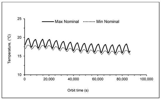
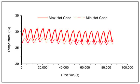
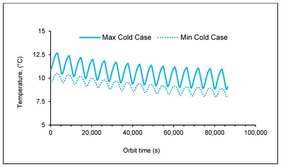
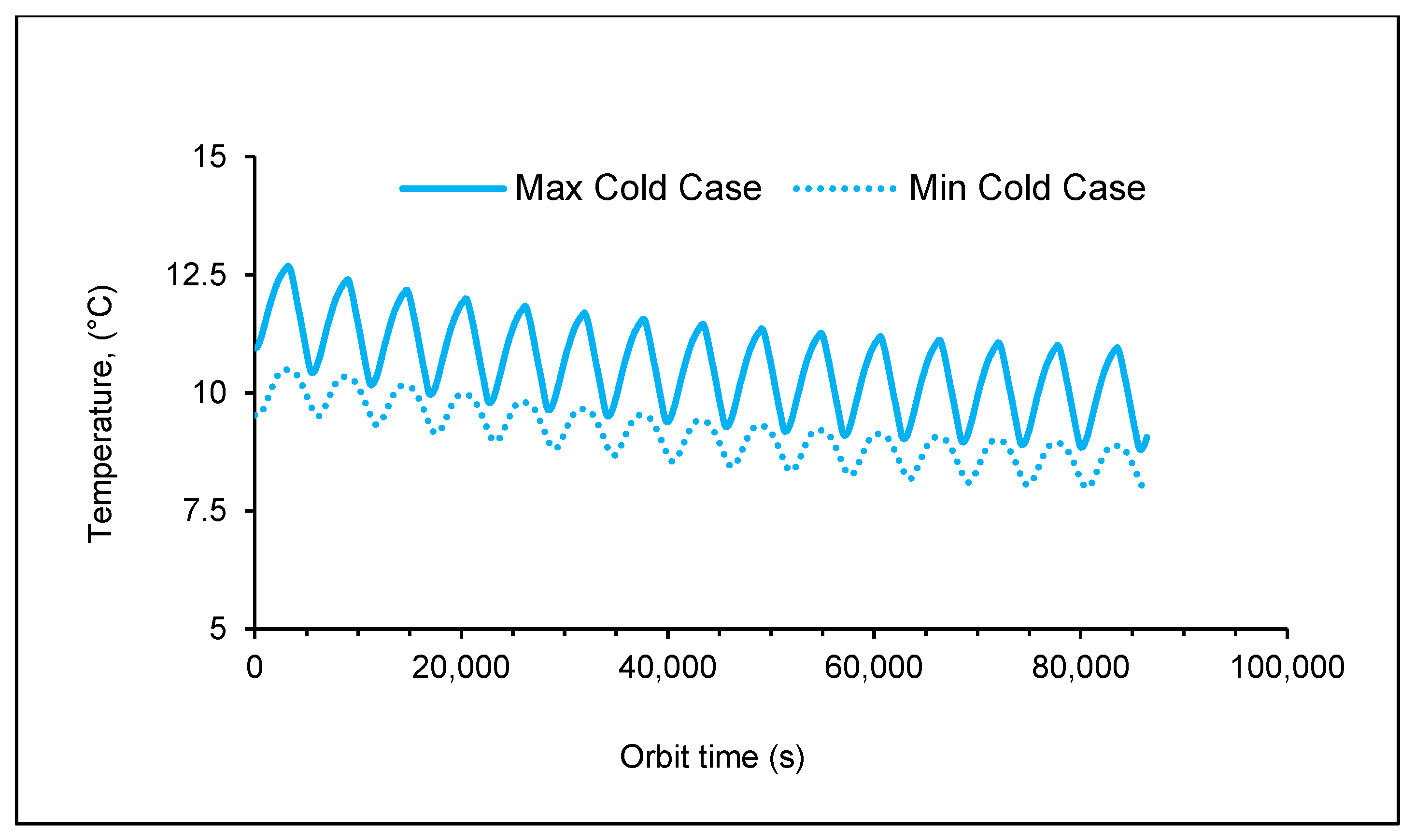
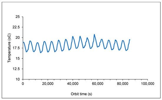
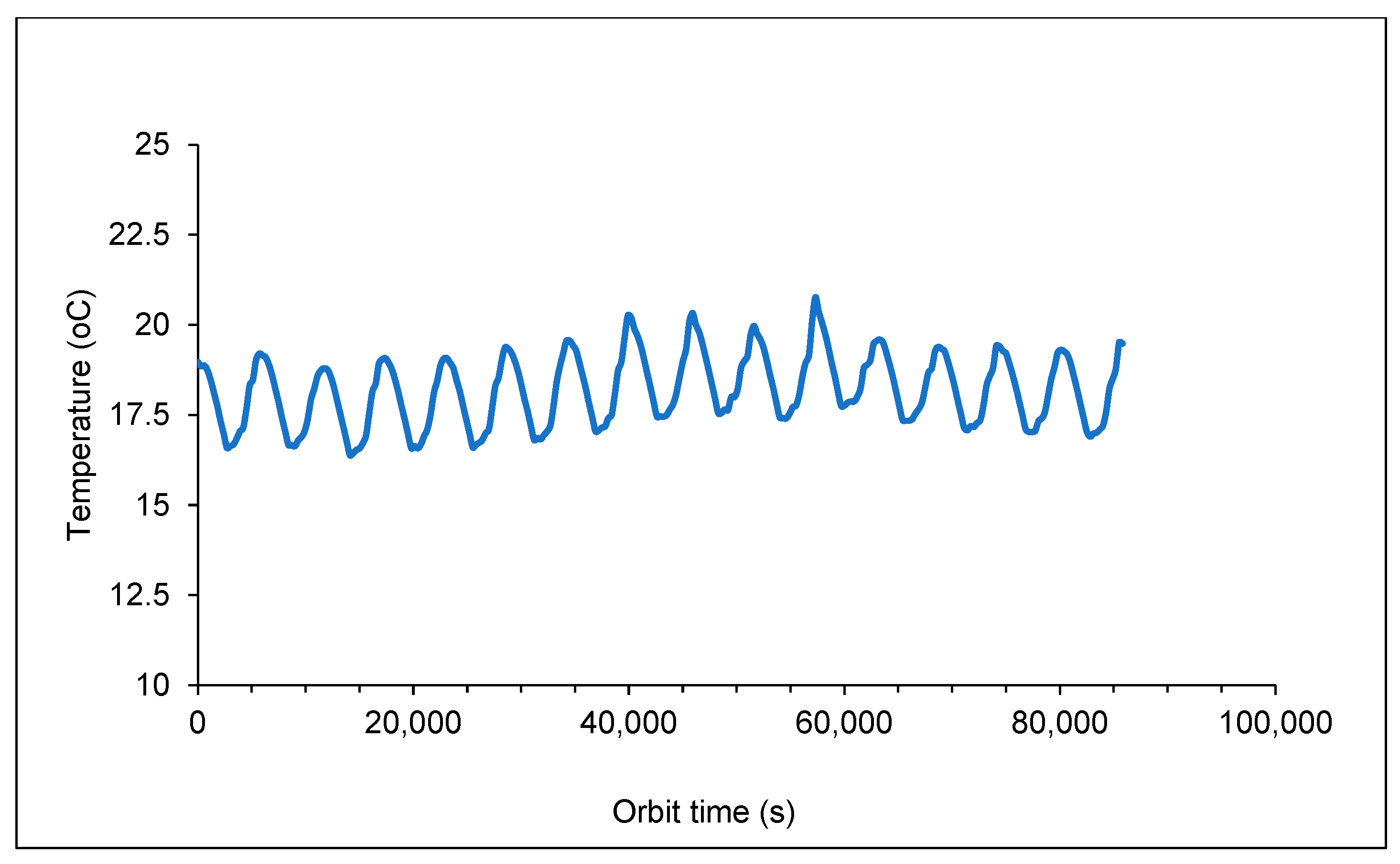
The thermal behaviour of the satellite’s subsystems was analysed and reported; however, this study focuses specifically on the thermal performance of the satellite batteries. Three operational scenarios—nominal, cold, and hot—were simulated to observe the influence of the space environment on the satellite batteries. The temperature distributions are presented over a 24 h orbital period. As illustrated in Figure 5, Figure 6 and Figure 7, the predicted temperature distributions are represented by two curves: the maximum and minimum temperature curves. The maximum curves indicate that the satellite is facing the sun, while the minimum curves represent the opposite (in shadow). The predicted temperatures are validated through comparison with real measurements obtained from the ground station [16] as well as with measured temperature values [14]. Under nominal conditions (Figure 5), the battery temperatures ranged from 15.40 °C for the minimum value to 19.4 °C for the maximum value. In the hot-case scenario (Figure 6), due to external thermal fluxes, higher temperature values were obtained, ranging from 26.6 °C to 30.9 °C for the minimum and maximum values. Conversely, in the cold case (Figure 7), the lower values of heat flux resulted in battery temperatures ranging from 7.9 °C to 12.2 °C for the minimum and maximum values. The battery temperature data (actual temperature values) collected from the ground-station observations are presented in Figure 8, indicating a range between 16.4 °C and 20.7 °C. As a result, all predicted and actual temperature values are within the acceptance range when compared with the operational (measured) temperatures, which fall between 10 °C and 30 °C [14]. It is evident that the predicted values in the cold-case scenario are lower than the operational temperature by 2.1 °C due to the worst-case assumption.

Figure 5. Predicted temperatures of the satellite battery for the nominal case.

Figure 6. Predicted temperatures of the satellite battery for the hot case.

Figure 7. Predicted temperatures of the satellite battery for the cold case.

Figure 8. Recorded real temperatures of the satellite battery during orbital operation from the KACST ground station [16].

4.2. Machine Learning Results

This section presents the results derived from applying ML models to predict satellite battery temperatures. The goal is to evaluate not only model performance but also practical applicability across various time frames and operational contexts.

4.2.1. Temporal Pattern Analysis

An exploratory analysis was conducted to investigate the temporal characteristics of battery temperature data and define baseline thermal behaviour before implementing predictive modelling. This step aimed to identify the dominant thermal cycles influencing battery temperature variation and quantify the thermal ranges that models must accurately forecast for operational reliability.

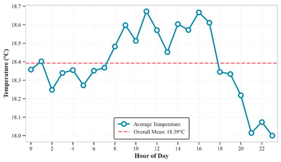
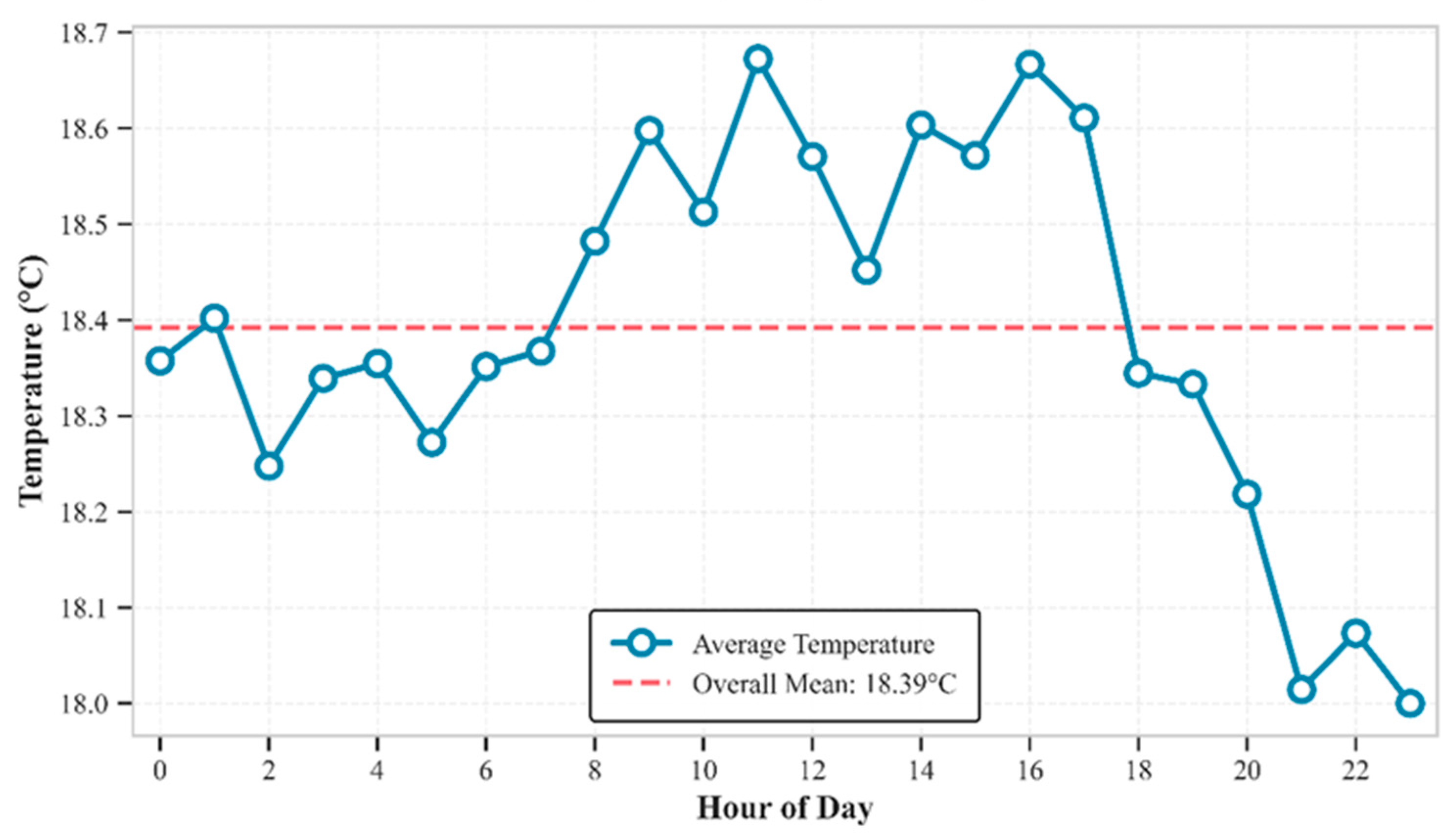
Average battery temperature, as shown in Figure 9 and aggregated hourly across the dataset, reveals minimal diurnal variation, fluctuating between 18.0 °C and 18.6 °C. A gradual increase is observed from the early morning hours, followed by a decline during the evening. The overall mean temperature remains stable at 18.4 °C.

Figure 9. Average battery temperature by hour.

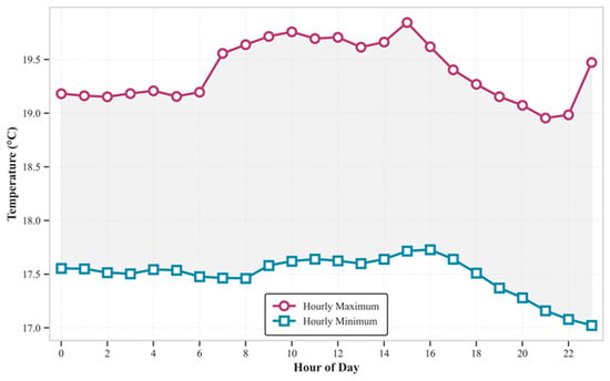
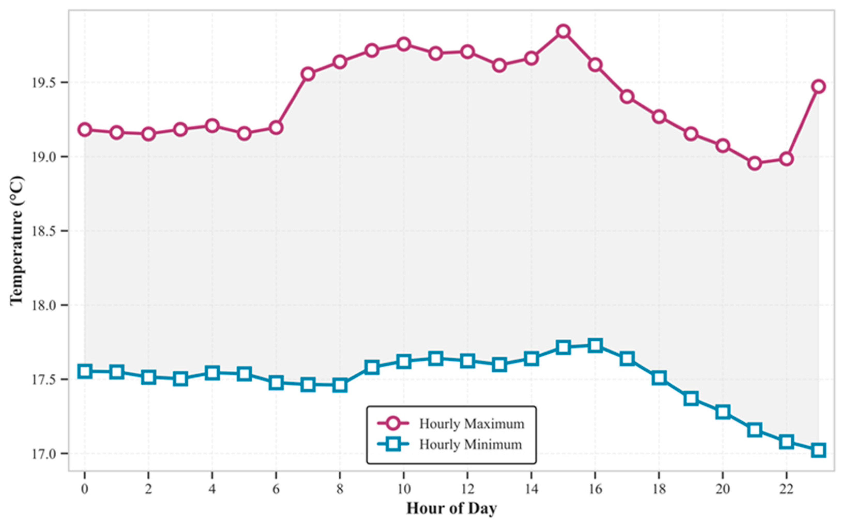
A sliding-window analysis was performed using one-hour windows consisting of 12 temperature measurements taken at five-minute intervals, reflecting typical operational forecasting horizons. For each window, the minimum and maximum temperatures were extracted to define the thermal envelope. As illustrated in Figure 10, the average hourly bounds show upper limits ranging from 19.0 °C to 19.8 °C and lower limits from 17.0 °C to 17.7 °C. The consistent separation of approximately 2.0 °C across all hours suggests rapid thermal cycling governed by orbital dynamics, rather than time-of-day effects. This consistent pattern suggests that temperature fluctuations are primarily driven by repeated transitions between heating and cooling phases during orbital movement.

Figure 10. Hourly temperature bounds.

This analysis establishes critical constraints for evaluating predictive models. Accurate forecasts must operate at sub-hourly resolution to capture short-term thermal variations and must predict not only average temperatures but also the thermal bounds within each forecast window. Deviations beyond historical bounds may signal thermal management anomalies or operational irregularities. The 2.0 °C average range defines a performance baseline, with acceptable prediction errors required to fall significantly below this threshold. These results clarify the thermal behaviour that models must learn, as well as outline the predictive standards necessary for reliable temperature forecasting in low-Earth-orbit satellite operations.

4.2.2. Model Performance Comparison

Three ML models—linear regression, Random Forest, and XGBoost—were evaluated for one-hour-ahead forecasting of satellite battery temperature. Performance was assessed using MAE, RMSE, and R² score, with the maximum absolute error (MaxAE) of these metrics calculated separately for the minimum and maximum values in each prediction window. The results are summarised in Table 5.

Table 5. Model performance comparison using MAE, RMSE, and R² for minimum and maximum predicted values.

Model	MAE Min	MAE Max	RMSE Min	RMSE Max	R2 Min	R2 Max	MaxAE Min	MaxAE Max
Li near Regression	0.201	0.233	0.266	0.330	0.983	0.976	1.83	1.988
Random Forest	1.057	0.724	1.2234	1.016	0.684	0.804	3.191	3.403
XGBoost	0.924	0.966	1.091	1.276	0.751	0.691	2.58	3.958

The results indicate that linear regression consistently outperformed the other models in both prediction accuracy and variance explanation. It achieved the lowest MAE and RMSE for both the minimum and maximum temperatures, with exceptionally high R² values (0.983 for minimum and 0.976 for maximum), suggesting a near-perfect fit to the data. This robust performance implies that the underlying temperature dynamics may exhibit linear characteristics over short-term forecasting horizons, which the linear model is adept at capturing.

In contrast, Random Forest and XGBoost, both ensemble-based models known for their ability to handle nonlinear relationships and complex interactions, did not perform as well in this task. Random Forest achieved moderate accuracy for maximum temperatures (MAE = 0.724 °C, R² = 0.804) but exhibited substantial error in predicting minimum temperatures (MAE = 1.057 °C, R² = 0.684), indicating reduced sensitivity to low-end thermal variations. XGBoost demonstrated a slightly better balance between minimum and maximum predictions than Random Forest, yet still lagged behind linear regression. Its performance metrics (e.g., RMSE = 1.091 °C for minimum temperatures and 1.276 °C for maximum) reflect difficulties in capturing the narrow thermal range (∼2.0 °C) and subtle fluctuations characteristic of the dataset. Consistent with the aggregate error metrics, the MaxAE values indicate that the largest individual deviation produced by linear regression remained below 2 °C for both targets, substantially lower than the corresponding values observed for the ensemble-based models (2.58–3.96 °C).

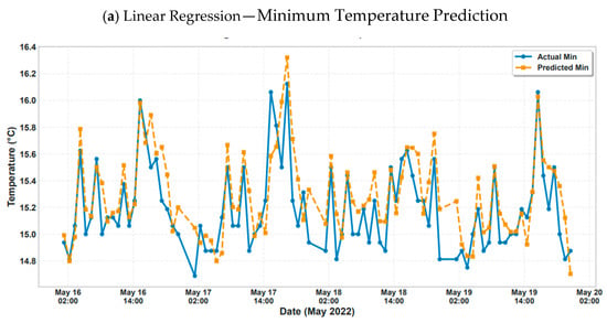
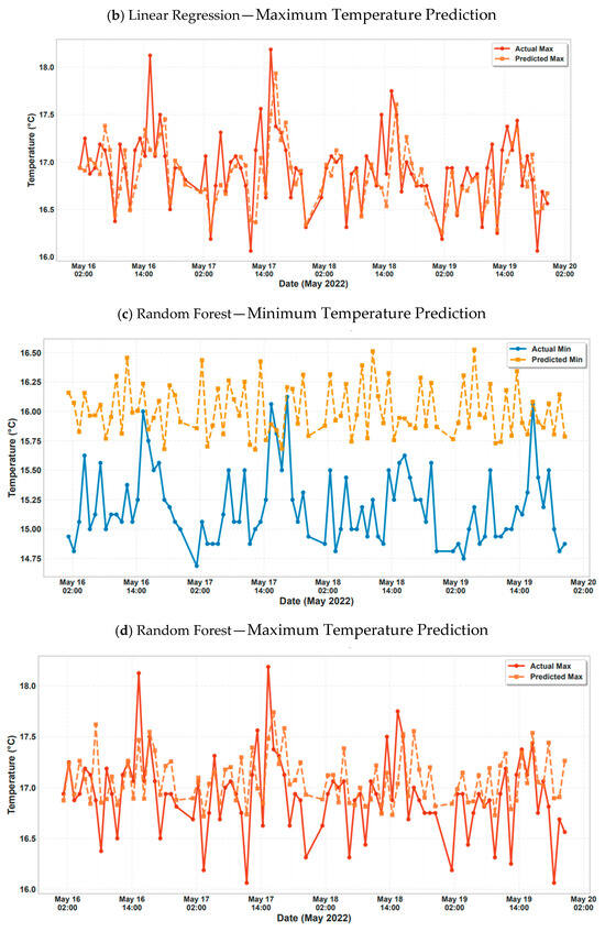
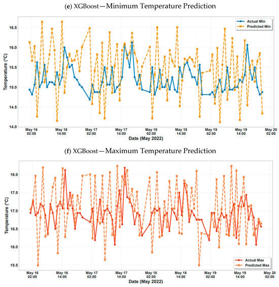
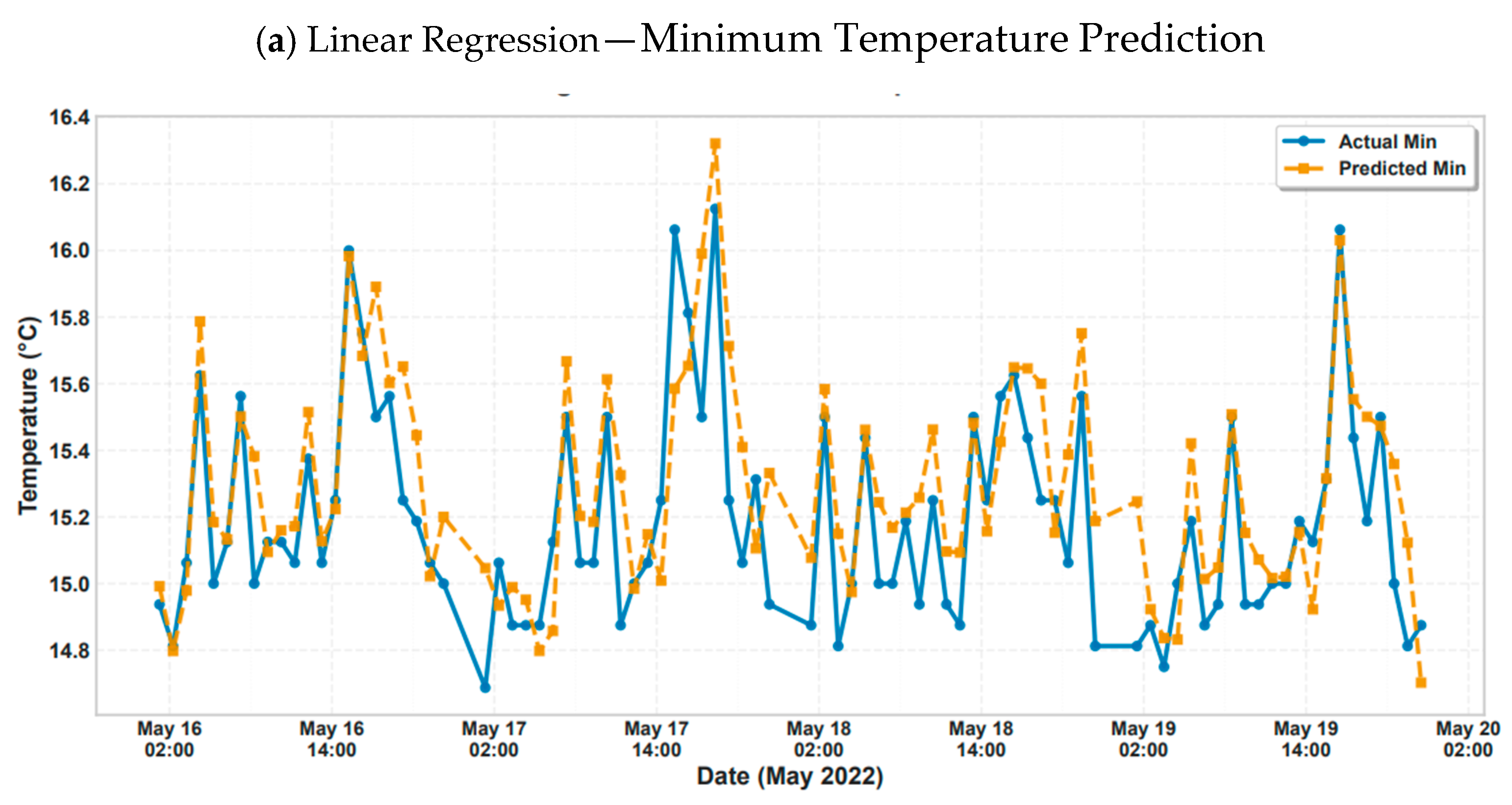
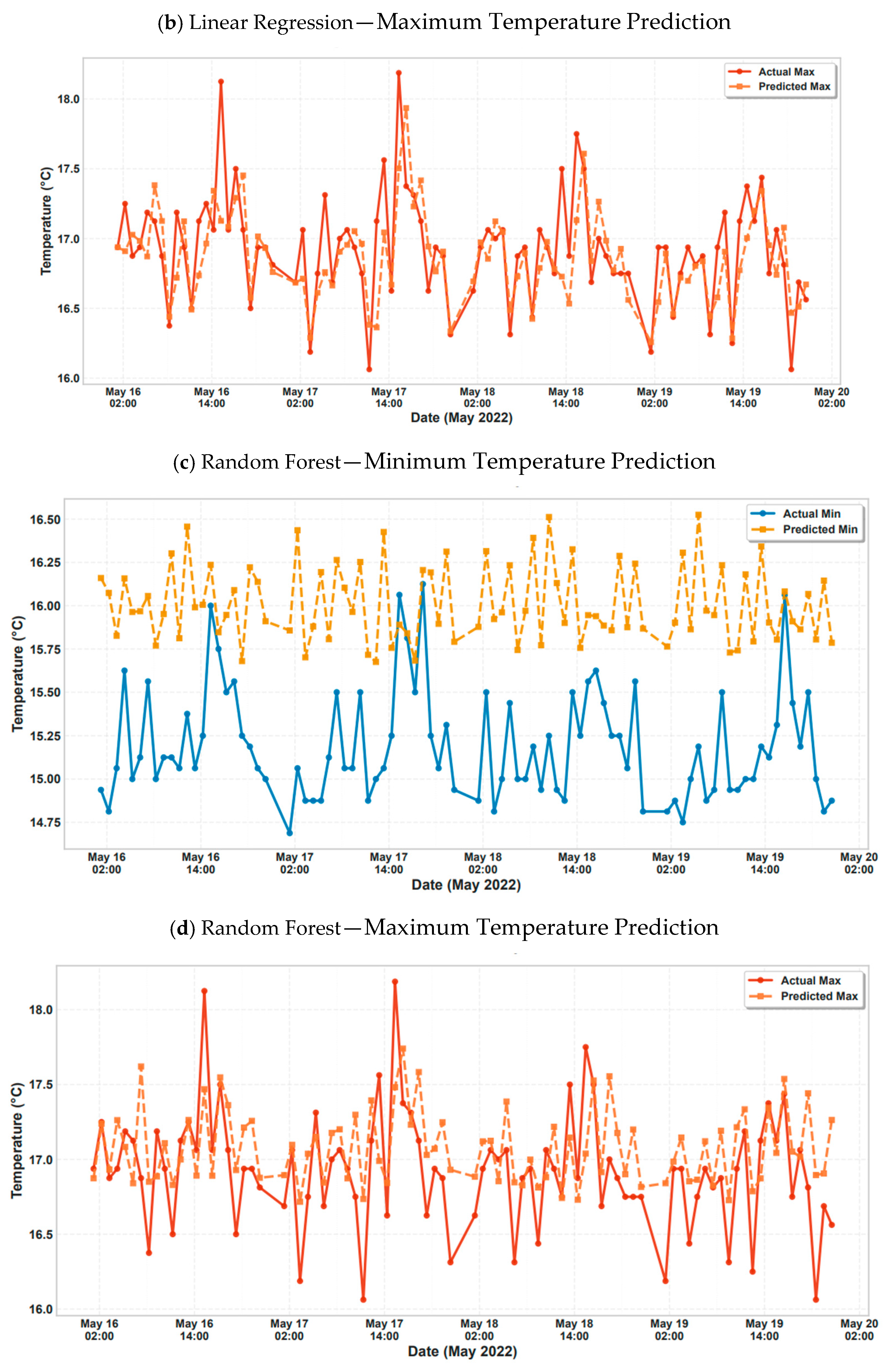
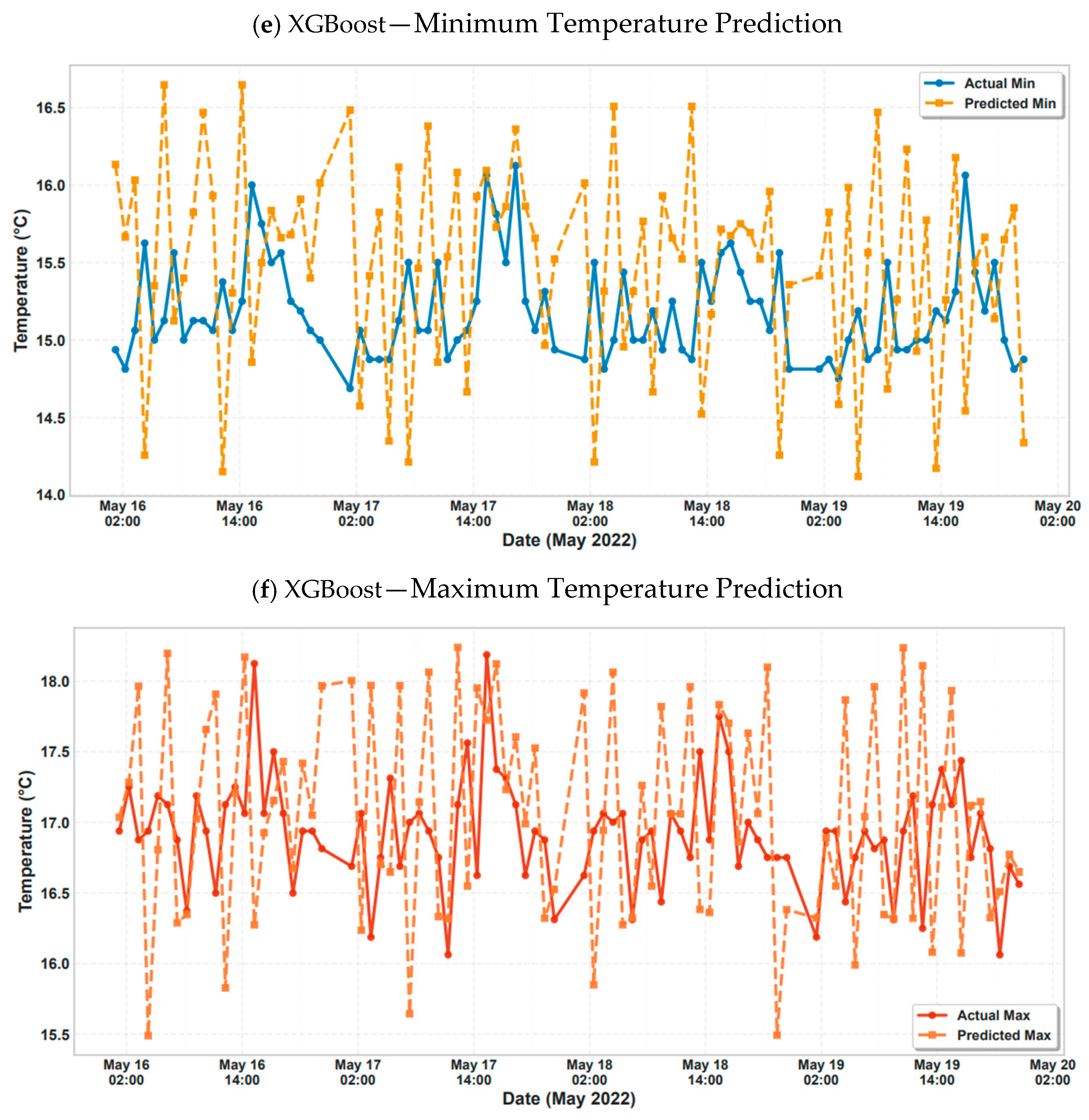
To further interpret these differences, a temporal segment from the test period (16–19 May 2022) was visualised to compare the predicted versus actual temperature extremes (Figure 11). This segment provides a detailed examination of how effectively each model tracks real-time changes.

Figure 11. Predicted vs. actual battery temperatures from 16 to 19 May 2022. (a,b) Linear regression; (c,d) Random Forest; (e,f) XGBoost.

As shown in Figure 11a,b, the linear regression predictions are closely aligned with the actual values for both the minimum and maximum temperatures, demonstrating their responsiveness to short-term variations and robustness throughout the observed range. Random Forest (Figure 11c,d), while adept at capturing broader trends, exhibited overestimation of minimum temperatures and smoothing effects that diminished precision. XGBoost (Figure 11e,f) frequently over- and under-predicted both extremes, displaying particularly poor sensitivity to rapid downward shifts in minimum temperatures.

These observations reinforce the numerical findings presented in Table 5. They further imply that model complexity does not necessarily translate to improved accuracy when the target variable exhibits constrained variation and minimal noise. In fact, the simplicity of linear regression appears to offer a better inductive bias for this forecasting problem, potentially due to the smooth, periodic nature of the battery temperature cycles driven by orbital dynamics. While ensemble models may offer advantages in scenarios with complex nonlinear interactions, their added complexity may hinder performance in narrowly bounded and relatively stable datasets. Linear regression emerged as the most reliable and interpretable model, meeting the key forecasting requirements—high precision, low variance, and robustness to short-term changes—all of which are critical for real-time thermal management in low-Earth-orbit satellite operations.

4.3. Comparison with Previous Studies

Previous studies have demonstrated the growing potential of machine learning for battery monitoring and spacecraft thermal management. For example, Safavi et al. [19] conducted a comparative evaluation of several machine learning algorithms for battery remaining-useful-life prediction and showed that model selection significantly influences prediction accuracy and computational efficiency. Although their work focused on battery degradation rather than thermal prediction, it similarly highlighted that selecting an appropriate learning algorithm is more important than simply adopting increasingly complex models. This observation is consistent with the findings of the present study, wherein the relatively simple linear regression model outperformed the more sophisticated Random Forest and XGBoost models for short-term satellite battery temperature prediction.

More recently, Jiang et al. [20] proposed a position-aware federated learning framework for satellite battery prediction using adaptive clustering and reinforcement learning. Their study demonstrated the potential of advanced distributed machine learning techniques for spacecraft battery monitoring. In contrast, the present work addresses a different problem by integrating conventional spacecraft thermal simulation, real in-orbit telemetry, and machine learning prediction within a unified framework. Rather than focusing on distributed learning, this study demonstrates that an interpretable and computationally efficient regression model can accurately predict satellite battery thermal behaviour while complementing traditional thermal analysis.

Overall, the findings suggest that increasing model complexity does not necessarily improve prediction performance for smooth orbital thermal behaviour. The proposed framework therefore provides a practical and computationally efficient solution for satellite battery thermal monitoring while preserving physical interpretability.

This study was validated using telemetry collected from a single low-Earth-orbit satellite operating under nominal mission conditions. Consequently, the reported model performance may vary for spacecraft employing different battery chemistries, thermal control architectures, orbital configurations, mission profiles, or telemetry sampling rates. Nevertheless, the proposed methodology is independent of a specific satellite platform and can be adapted to future missions by retraining the prediction models using mission-specific telemetry data. Future work will investigate multi-satellite datasets, additional operational parameters, and advanced hybrid physics-informed machine learning approaches.

4.4. Case Study

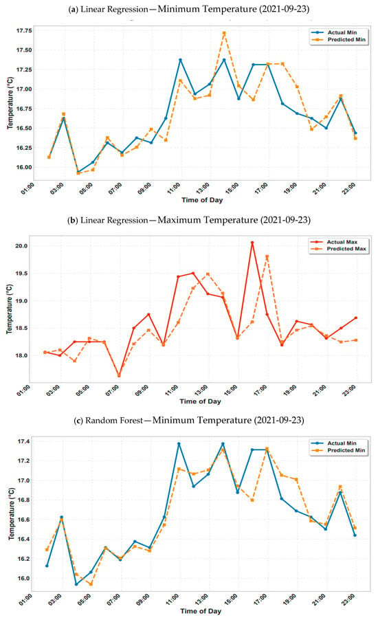
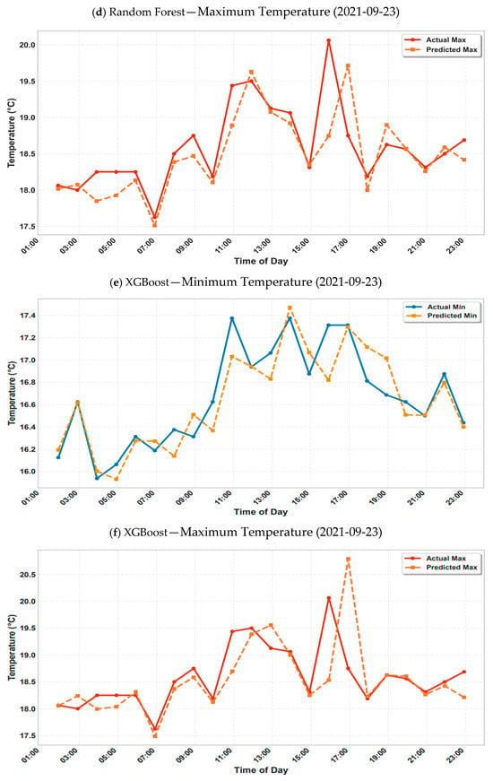
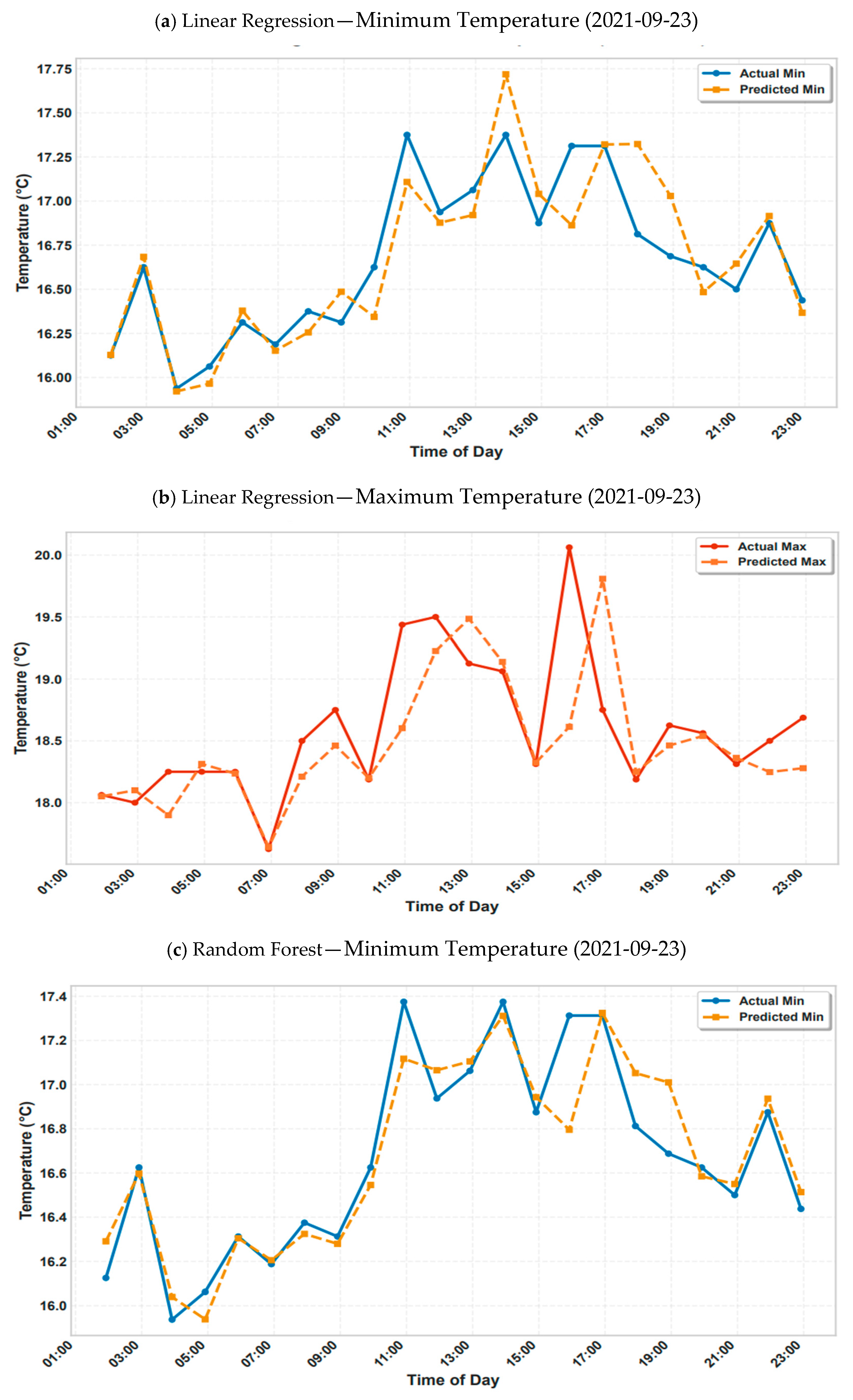
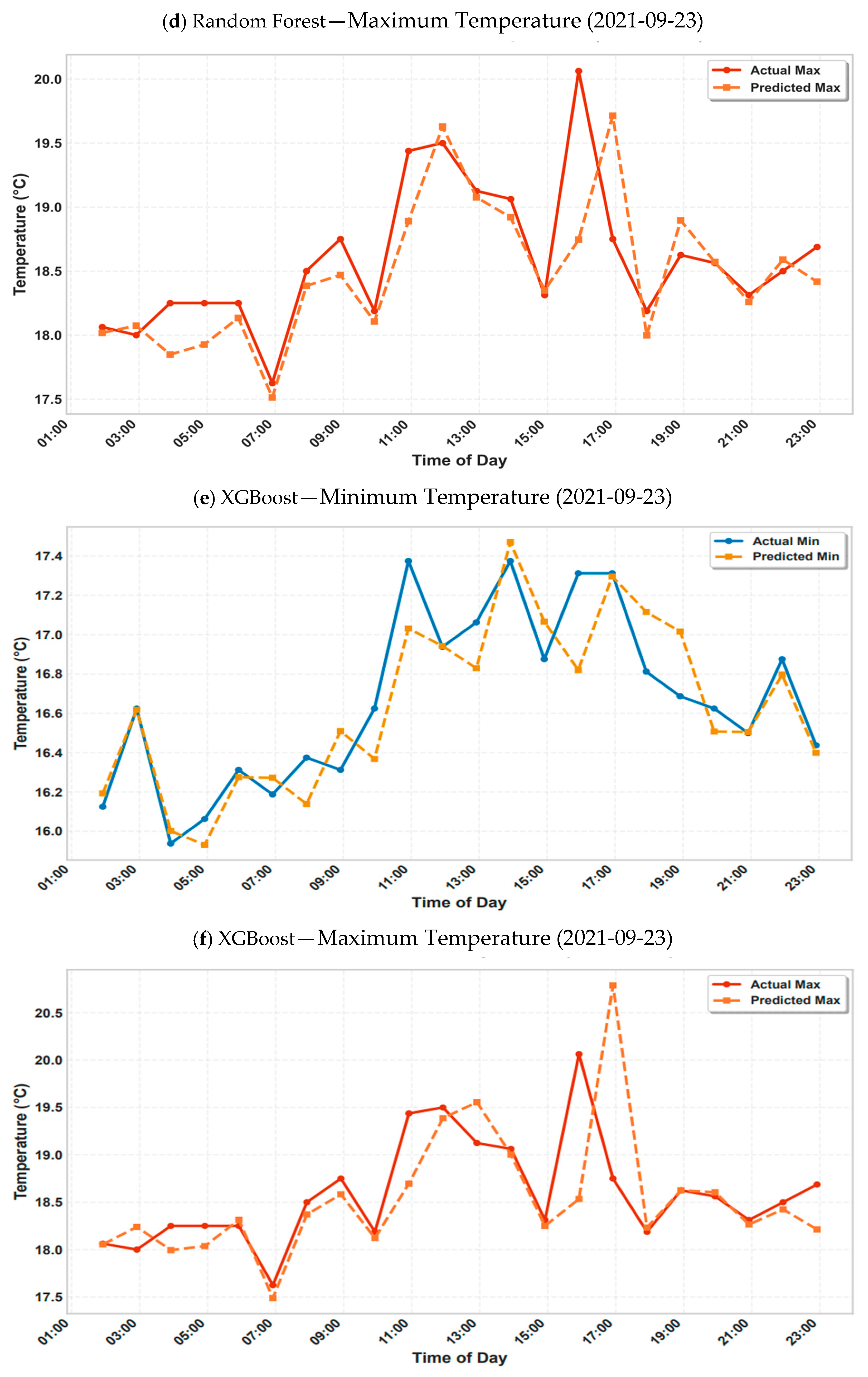
The generalisation capability and reliability of the trained ML models were evaluated using a case study conducted on 23 September 2021, a date that was excluded from the training set. This ensures that the evaluation reflects a realistic prediction scenario, free from data leakage or overfitting. The ML models were used to forecast one-hour-ahead extremes in battery temperature using only preceding data, simulating real-time operational forecasting.

Figure 12 illustrates the predicted minimum and maximum battery temperatures on this date across all ML models. Among them, linear regression clearly demonstrates the closest alignment with the actual values, accurately capturing both the magnitude and timing of thermal fluctuations. This result reinforces its status as the most reliable model among those tested.

Figure 12. Case study predicted vs. actual battery temperatures from 23 September 2022. (a,b) Linear regression; (c,d) Random Forest; (e,f) XGBoost.

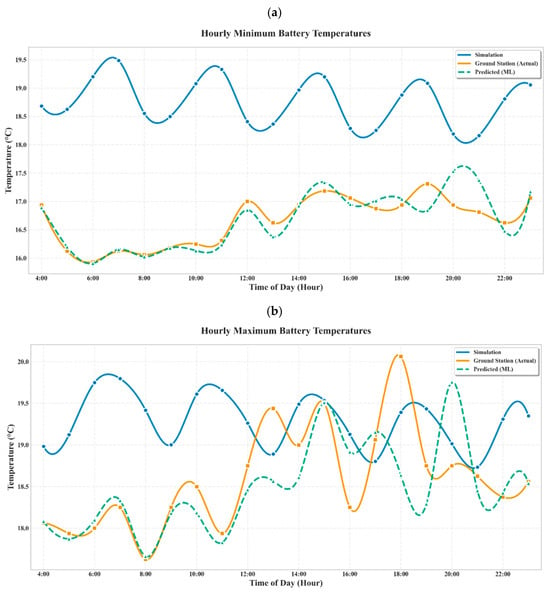
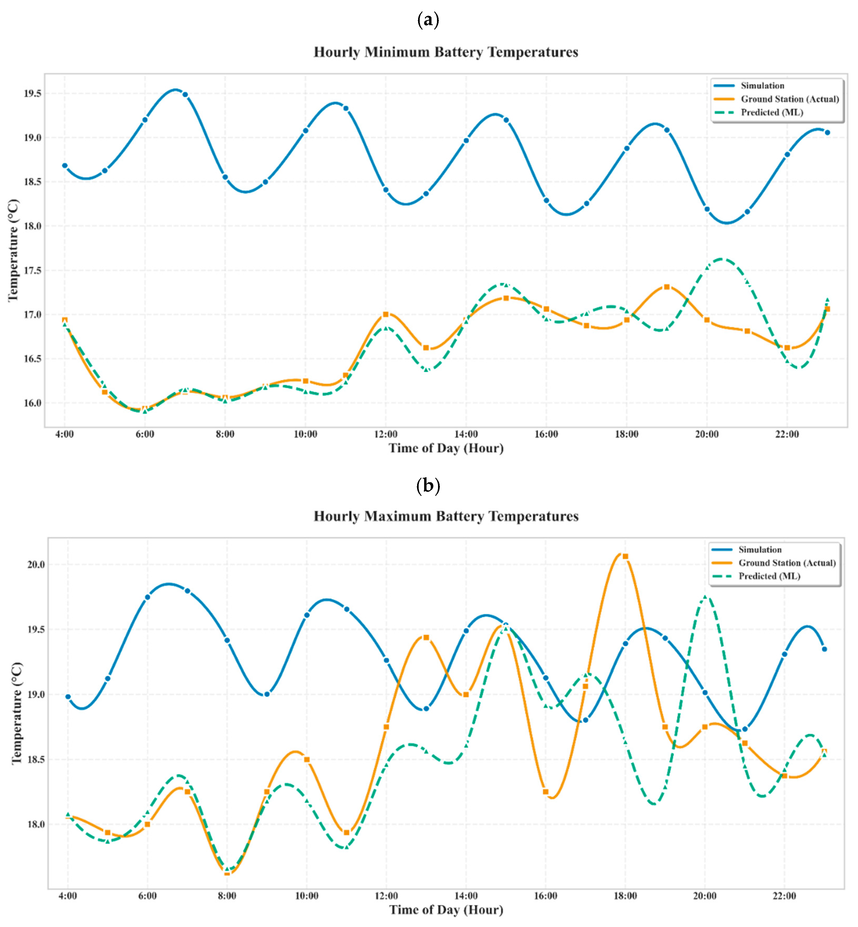
Subsequently, the output from the linear regression model was compared to the simulation-based thermal estimates, which are traditionally used for satellite thermal planning. As shown in Figure 13, the simulation reproduces the broad temperature trend but fails to match the true peaks and troughs, particularly during dynamic transition periods (e.g., eclipse entry/exit or load-induced fluctuations).

Figure 13. Hourly battery temperature predictions: (a) minimum and (b) maximum temperatures from simulation (blue circles); actual ground-station data (orange squares); and linear regression model (teal triangles, dashed).

The linear regression model consistently outperforms the simulation, especially in capturing the fine-grained structure of temperature variability. This advantage is attributed to the use of a sliding input window of 12 historical points (equivalent to one hour), which provides sufficient context for modelling short-term thermal dynamics. Unlike the simulation, which is governed by static equations and idealised assumptions, the data-driven model adapts to recent behavioural patterns and environmental interactions.

5. Conclusions

This paper presents the temperature performance of satellite batteries in space by employing thermal analysis, real battery temperature data, and ML predictions. The thermal analysis was performed through the FEMAP version 11.3 software programme in three different scenarios: hot, cold, and nominal conditions. The real data of the batteries were collected from the satellite ground station.

The ML models applied in this study are linear regression, Random Forest, and XGBoost. These models were assessed using metrics such as MAE, RMSE, and R², which were computed for each prediction window for the minimum and maximum temperatures. A temporal error analysis was conducted for further evaluation of the models’ prediction performance. The primary aim of the study was to assess the influence of the space environment on battery thermal behaviour and evaluate whether ML-based forecasts can serve as reliable operational complements or supplements to simulation models.

The findings indicate that the linear regression model outperformed the other ML approaches, achieving the highest R² (0.976) and the lowest MAE (0.20 °C), indicating strong accuracy and generalisation capability. A detailed case study for an unseen date (23 September 2021) further validated the linear regression model, demonstrating its ability to capture real-time thermal patterns more accurately compared to the simulation. While the simulation provides a broad approximation, it exhibited a greater deviation from actual data during dynamic orbital transitions. In contrast, the ML model—trained on sliding windows of recent data—adapted effectively to local temperature trends and demonstrated better agreement with ground-station measurements.

All ML-predicted temperature values remained within the operational acceptance range established by the measured data (10 °C to 30 °C). Maintaining the battery temperature within this range is critical for ensuring long-term reliability and performance, supporting the claim that ML forecasting can contribute to more informed and thermally secure mission planning.

The proposed framework demonstrates that machine learning should be regarded as a complement rather than a replacement for conventional thermal simulation. By integrating physics-based thermal modelling with operational telemetry, the proposed approach provides an efficient and interpretable framework for real-time spacecraft thermal monitoring. Future work will extend the framework to multiple satellite platforms, incorporate additional environmental and operational variables, and investigate hybrid physics-informed machine learning models for enhanced prediction robustness.

References

- Jaluria, Y. Challenges in the accurate numerical simulation of practical thermal processes and systems. Int. J. Numer. Methods Heat Fluid Flow 2013, 23, 158–175. [Google Scholar] [CrossRef] [Scilit]
- d’Alessandro, V.; Rinaldi, N. A critical review of thermal models for electro-thermal simulation. Solid-State Electron. 2002, 46, 487–496. [Google Scholar] [CrossRef] [Scilit]
- Jordan, M.I.; Mitchell, T.M. Machine learning: Trends, perspectives, and prospects. Science 2015, 349, 255–260. [Google Scholar] [CrossRef] [Scilit] [PubMed]
- Girimonte, D.; Izzo, D. Artificial intelligence for space applications. In Intelligent Computing Everywhere; Schuster, A.J., Ed.; Springer: London, UK, 2007; pp. 235–253. [Google Scholar] [CrossRef] [Scilit]
- Rao, G.M.; Pandipati, R.C. Satellites: Batteries. In Encyclopedia of Electrochemical Power Sources; Elsevier: Amsterdam, The Netherlands, 2009; pp. 323–337. [Google Scholar]
- Knap, V.; Vestergaard, L.K.; Stroe, D.I. A review of battery technology in CubeSats and small satellite solutions. Energies 2020, 13, 4097. [Google Scholar] [CrossRef] [Scilit]
- Ahmed, A.M.; Salama, A.; Ibrahim, H.A.; Sayed, M.A.E.; Yacout, S. Prediction of battery remaining useful life on board satellites using logical analysis of data. In Proceedings of the 2019 IEEE Aerospace Conference, Big Sky, MT, USA, 2–9 March 2019; IEEE: Piscataway, NJ, USA, 2019; pp. 1–8. [Google Scholar]
- De Canio, G.; Boumghar, R.; Godard, T.; Weissmann, U. Optimization of the battery usage during eclipses using a machine learning approach. In Proceedings of the 2018 SpaceOps Conference, Marseille, France, 28 May–1 June 2018; American Institute of Aeronautics and Astronautics (AIAA): Reston, VA, USA, 2018; Paper 2607. [Google Scholar]
- Donato, T.H.R. Machine Learning Systems Applied in Satellite Lithium-Ion Battery Set Impedance Estimation. Master’s Thesis, Instituto Nacional de Pesquisas Espaciais (INPE), São José dos Campos, Brazil, 2018. [Google Scholar]
- Alburayt, A.I.; Alharbi, M.A.; Alturky, M.A.; Alhossaini, O.S.; Alattas, Y.H. A comparative study of satellite battery performance in space environment. In Proceedings of the 11th International Conference on Mechanical, Automotive and Materials Engineering (CMAME 2024); Lecture Notes in Mechanical Engineering; Springer: Singapore, 2026. [Google Scholar] [CrossRef] [Scilit]
- Alshamlan, N.; Alharbi, M.A.; Alburayt, A.I.; Alattas, Y.H.; Alturky, M.A. Real and predicted temperature distributions of LEO satellite attitude determination and control system (ADCS). In Proceedings of the International Conference on Mechanical, System and Control Engineering, Singapore, 2024; Springer Nature: Singapore, 2024; pp. 125–131. [Google Scholar]
- Kamul, A.; Hananda, N.; Harito, C.; Djuana, E.; Elwirehardja, G.N.; Pardamean, B.; Gunawan, F.E.; Budiman, A.S.; Asrol, M.; Redi, A.P.; et al. Machine learning application in battery prediction: A systematic literature review and bibliometric study. E3S Web Conf. 2023, 388, 01021. [Google Scholar] [CrossRef] [Scilit]
- Siemens Digital Industries Software. Femap Version 11.3.2. Available online: https://blogs.sw.siemens.com/simcenter/femap-version-11-3-2/ (accessed on 30 July 2026).
- ABSL. Available online: https://absl.pl/en (accessed on 30 July 2026).
- Gilmore, D.G. Spacecraft Thermal Control Handbook. Volume 1: Fundamental Technologies; Aerospace Press: El Segundo, CA, USA, 2002. [Google Scholar]
- King Abdulaziz City for Science and Technology (KACST). Ground Station. Available online: https://kacst.gov.sa/ (accessed on 30 July 2026).
- Pang, J.; Liu, D.; Peng, Y.; Peng, X. Anomaly detection for satellite telemetry series with prediction interval optimization. In Proceedings of the 2018 International Conference on Sensing, Diagnostics, Prognostics, and Control (SDPC), Xi’an, China, 15–17 August 2018; IEEE: Piscataway, NJ, USA, 2018; pp. 408–414. [Google Scholar]
- Sachan, P.; Bharadwaj, P. Incorporating uncertainty and reliability for battery temperature prediction using machine learning methods. IEEE J. Emerg. Sel. Top. Ind. Electron. 2024, 5, 234–241. [Google Scholar] [CrossRef] [Scilit]
- Safavi, V.; Mohammadi Vaniar, A.; Bazmohammadi, N.; Vasquez, J.C.; Guerrero, J.M. Battery remaining useful life prediction using machine learning models: A comparative study. Information 2024, 15, 124. [Google Scholar] [CrossRef] [Scilit]
- Jiang, S.; Wang, B.; Zhang, X.; Jiang, Y.; Liu, S.; Zhao, Z.; Li, R.; Chen, X. ObsBattery: Position-aware federated learning with dueling DQN clustering and training adaptation for satellite battery prediction. Electronics 2025, 14, 4697. [Google Scholar] [CrossRef] [Scilit]
Disclaimer/Publisher’s Note: The statements, opinions and data contained in all publications are solely those of the individual author(s) and contributor(s) and not of MDPI and/or the editor(s). MDPI and/or the editor(s) disclaim responsibility for any injury to people or property resulting from any ideas, methods, instructions or products referred to in the content. |
© 2026 by the authors. Licensee MDPI, Basel, Switzerland. This article is an open access article distributed under the terms and conditions of the Creative Commons Attribution (CC BY) license.