


Abstract
Forecasting agricultural futures prices across multiple commodities remains highly challenging due to nonlinear price dynamics, strong market volatility, and complex cross-market and cross-commodity interactions. To address these issues, this paper proposes an explainable ensemble forecasting framework that integrates cross-market feature construction and interpretation, a benchmark forecasting model pool, and reinforcement learning-based ensemble optimization. A diverse set of deep learning models generate benchmark forecasts using cross-market features that contain effective information, and a reinforcement learning-guided chaotic evolutionary optimization algorithm is employed to dynamically determine the ensemble weights under a multi-objective criterion that balances prediction accuracy and stability. Meanwhile, explainable artificial intelligence techniques, including SHAP and LIME, are incorporated to analyze the contribution of cross-market features to price predictions. The proposed framework is applied to eight major agricultural futures markets, including wheat, corn, and soybean-related commodities. Empirical results show that the ensemble model consistently outperforms individual forecasting models in terms of prediction accuracy and stability. Moreover, in backtesting, most agricultural commodities achieve positive returns under controlled risk levels. The findings indicate that the proposed framework not only improves predictive performance and generates substantial returns for most commodities, but also provides interpretable insights into the mechanisms linking financial markets and agricultural commodity prices, demonstrating its potential value for forecasting, trading, and risk management applications.
1. Introduction
Agricultural futures markets play a crucial role in the global food supply chain and financial system. Prices of major agricultural commodities such as wheat, corn, and soybeans influence not only agricultural production and trade but also global food security and macroeconomic stability. Accurate forecasting of agricultural futures prices is therefore essential for market participants, including producers, traders, and policymakers. However, forecasting agricultural futures prices across multiple commodities remains highly challenging due to strong market volatility, nonlinear price dynamics, and complex cross-market interactions. These characteristics motivate the development of forecasting frameworks that can simultaneously achieve high predictive accuracy, robustness, and interpretability.
Early research on agricultural price forecasting primarily relied on traditional econometric and time-series models. Classical approaches such as autoregressive integrated moving average (ARIMA) and generalized autoregressive conditional heteroskedasticity (GARCH) have been widely used to model temporal dependence and volatility clustering. In the agricultural economics literature, these models have been extensively applied to commodity price forecasting. For example, Ahumada and Cornejo [1] examine forecasting performance for major agricultural commodities including corn, soybeans, and wheat, while Etienne et al. [2] develop a futures-based forecasting framework for U.S. corn prices. Other studies incorporate additional explanatory variables, such as online search behavior, to enhance predictive performance [3]. Although these econometric models provide interpretable structures and solid theoretical foundations, their linear assumptions limit their ability to capture nonlinear patterns and high-dimensional interactions in modern financial markets.
Traditional time-series models still have considerable value in empirical applications, offering distinct advantages in capturing temporal dependence, autocorrelation, and conditional heteroskedasticity, while also serving as important benchmarks for evaluating other forecasting approaches. ARIMA-type models primarily capture linear temporal structures and short-run persistence, whereas GARCH-family models are well suited to describing volatility clustering and time-varying conditional risk. These properties are particularly relevant in agricultural futures markets, where prices are influenced by persistent trends as well as abrupt changes in market uncertainty. Recent empirical evidence confirms that traditional models remain competitive under specific conditions. For example, Wang et al. [4] combine ARIMA with nonlinear machine learning models and denoising techniques to forecast corn and soybean futures prices, finding that forecast combinations substantially reduce prediction errors relative to individual models. Similarly, a recent comparative study across major agricultural commodities shows that ARIMA can provide stable short-horizon forecasts during relatively low-volatility periods, although nonlinear deep learning models tend to perform better during highly volatile episodes [5]. At the same time, their limitations in handling more complex dependencies explain the need to shift toward nonlinear machine learning and deep learning approaches.
With the rapid development of machine learning and artificial intelligence, data-driven approaches have become increasingly prominent in commodity price forecasting. Machine learning models are capable of capturing nonlinear relationships and complex interactions among multiple variables. More recently, deep learning architectures have demonstrated strong performance in modeling sequential data with long-term dependencies. In particular, recurrent neural networks such as long short-term memory (LSTM) have been widely used in financial forecasting tasks [6], while hybrid architectures such as CNN–LSTM further improve predictive performance by combining spatial and temporal feature extraction [7]. A comprehensive review by Sezer and Ozbayoglu [8] highlights the effectiveness of deep learning methods in financial time series forecasting and emphasizes the importance of integrating multiple data sources in complex market environments.
Despite the success of deep learning models, relying on a single model often leads to unstable predictions due to model-specific biases and overfitting. Ensemble learning has therefore emerged as an effective strategy to improve forecasting performance by combining multiple models. Theoretical and empirical studies have shown that ensemble methods can enhance generalization ability and reduce prediction errors by aggregating complementary information from heterogeneous models. For example, Patel et al. [9] demonstrate that hybrid and ensemble approaches significantly improve stock market prediction accuracy, while Ganaie et al. [10] provide a comprehensive review of ensemble deep learning methods and their advantages in complex prediction tasks. These findings suggest that ensemble frameworks are particularly suitable for financial forecasting problems characterized by high uncertainty and structural complexity.
Forecasting performance of traditional econometric, machine learning, and deep learning models often varies with market conditions and the underlying data-generating process. Recent research no longer emphasizes replacing traditional methods with new ones, but rather focuses on combining different types of models to more efficiently exploit data. In forecasting agricultural commodity prices, such combinations can leverage both the linear relationships captured by econometric models and the nonlinear patterns extracted by machine learning and deep learning models [4]. This provides a fundamental rationale for ensemble forecasting: different models have complementary strengths in revealing various aspects of price dynamics, and combining them can make the fullest use of predictive information, thereby improving forecasting performance while reducing the prediction bias and overfitting issues associated with individual models. However, ensemble forecasting also introduces increased complexity, making it more difficult to determine which input variables drive the final output and why the model behaves differently across market conditions. As a result, our attention naturally shifts from predictive accuracy alone to model interpretability, motivating the incorporation of XAI methods into the forecasting framework.
In parallel with advances in predictive modeling, explainable artificial intelligence (XAI) has become increasingly important in the field of financial forecasting. Although deep learning and ensemble methods often achieve high predictive accuracy, their lack of interpretability has always limited their application in financial decision-making. To address this issue, researchers have developed methods such as local interpretable model-agnostic explanations (LIME) [11] and SHapley Additive exPlanations (SHAP) [12], which can provide both local and global explanations of model predictions. Empirical studies in finance have confirmed the practical value of these techniques: Gramegna and Giudici [13] find that SHAP and LIME effectively extract discriminative feature contributions from complex credit risk models, while Çelik et al. [14] integrate LIME into financial time series ensemble forecasting to assess prediction reliability and support decision-making. Recent research has further extended Shapley-based explanations to neural network architectures for time series [15], and has combined SHAP with Transformer models to achieve fine-grained interpretability of historical time steps and input features [16].
Interpretability does not necessarily come at the cost of predictive accuracy. Giudici et al. [15] evaluate neural-network-based time-series models with respect to accuracy, robustness, and interpretability, and find that recurrent architectures substantially outperform simpler benchmarks on both accuracy and robustness while remaining amenable to Shapley-based interpretation. Recently, Hertel et al. [16] proposed SHAPformer, which integrates SHAP-based explanations directly into the Transformer forecasting framework. Their experiments show that this model maintains competitive predictive accuracy while providing precise local and global explanations; on the electricity price dataset, SHAPformer even outperforms the standard Transformer and other benchmark models. Interpretability and predictive performance are not conflicting objectives. By combining XAI with neural network models, we can obtain interpretable predictive information. Furthermore, a recursive forecasting structure can continuously refine the usefulness of input information, thereby both enhancing model transparency and maintaining or even further improving predictive accuracy.
Comprehensive surveys also confirm that SHAP, feature importance analysis, and attention mechanisms have become the most common XAI strategies in financial time series forecasting [17]. Overall, XAI is evolving from a post-hoc interpretation tool into a crucial bridge between predictive models and financial decision-making: global explanations help us identify persistently influential variables that drive market dynamics, while local explanations help reveal feature contributions under specific market conditions, assisting researchers in understanding model behavior during abnormal episodes. Motivated by these advances, this study employs SHAP for global feature importance analysis to identify the overall contributions of macro-financial variables to ensemble predictions, and uses LIME for local explanations of representative prediction instances, thereby enhancing the transparency and interpretability of the proposed ensemble forecasting framework.
Despite these advances, several important limitations remain in the existing literature. First, most studies focus on forecasting a single commodity market in isolation, while agricultural futures markets are inherently interconnected through global trade, substitution effects, and shared macroeconomic drivers. As a result, cross-market information is often underutilized in forecasting models. Second, many existing ensemble approaches rely on static weighting schemes, which cannot adapt to changing market conditions and may fail to capture dynamic relationships among forecasting models. Third, although explainable AI methods have been widely applied in various domains, their integration into ensemble forecasting frameworks for agricultural futures markets remains limited, and few studies simultaneously address predictive accuracy and interpretability within a unified framework.
To address these limitations, this paper proposes an explainable ensemble forecasting framework for agricultural futures prices based on a reinforcement learning-guided chaotic evolutionary optimization algorithm. The proposed framework integrates cross-market feature construction, a heterogeneous pool of deep learning models, and a dynamic ensemble optimization mechanism. Specifically, cross-market features are constructed to capture interactions among macro-financial variables and commodity markets. Multiple deep learning architectures are then employed to generate individual forecasts, and a reinforcement learning-guided multi-objective optimization algorithm is used to dynamically determine ensemble weights. Finally, SHAP and LIME are incorporated to provide both global and local interpretability, thereby enhancing model transparency and identifying key drivers of agricultural futures price dynamics.
This paper makes three main contributions. First, it extends agricultural futures forecasting from a single-market setting to a multi-commodity framework by incorporating cross-market features, enabling the model to capture information spillovers across markets. Second, it develops a dynamic ensemble forecasting framework in which multiple neural network models are combined using a reinforcement learning-guided optimization algorithm, improving both predictive accuracy and stability. Third, it integrates explainability analysis into the ensemble framework through SHAP and LIME, providing insights into the underlying mechanisms of price formation and enhancing the interpretability of forecasting results.
The remainder of this paper is organized as follows. Section 2 describes the dataset and preprocessing procedures. Section 3 presents the proposed methodology. Section 4 reports the empirical results. Section 5 evaluates the economic value of the forecasts. Section 6 provides robustness checks. Section 7 concludes the study.
2. Data
2.1. Agricultural Futures Markets and Data Sources
This study selects eight representative agricultural futures contracts traded on major international exchanges as research objects for agricultural futures price forecasting. The dataset includes London Wheat, U.S. Rough Rice, U.S. Corn, U.S. Wheat, U.S. Soybean, U.S. Soybean Meal, U.S. Soybean Oil, and China Soybean No. 2. These varieties represent key commodities in agricultural trade and are widely used by producers, speculators, and financial institutions for hedging and speculative purposes.
Most of the selected varieties are traded on the Chicago Board of Trade (CBOT), which plays a central role in global agricultural price discovery and therefore serves as the primary focus of this study. Contracts such as rough rice, corn, wheat, soybeans, soybean meal, and soybean oil are among the most liquid agricultural derivatives markets, providing rich information about supply–demand expectations and global agricultural price dynamics. Their high liquidity and transparency also create favorable conditions for empirical analysis. Meanwhile, the dataset also incorporates varieties from other markets to validate the cross-market influence of macro-financial variables. London Wheat futures represent an important European benchmark for wheat pricing, while China Soybean No. 2 futures are included to capture regional market dynamics from China, one of the world’s largest soybean importers. By covering both Western and Chinese markets, this study captures price dynamics across different agricultural markets and measures the impact of macro-financial variables on agricultural futures prices across different markets and varieties.
Based on these eight agricultural futures varieties, this study constructs a dataset consisting of daily historical observations collected from major commodity exchanges and financial data providers. In addition to futures market data, to further capture cross-market influences on agricultural commodity prices, the dataset incorporates multiple categories of macro-financial variables, specifically covering five dimensions: monetary policy, equity markets, market sentiment, geopolitical risk, and commodity markets. Detailed descriptions of each variable and their corresponding data sources are summarized in Table 1.
Table 1.
Influencing factors of agricultural futures price fluctuations.
The selection of macro-financial indicators in this study draws on established empirical literature on commodity price dynamics and forecasting. Specifically, the Dollar Index captures exchange rate conditions that affect the international competitiveness and dollar-denominated valuation of agricultural commodities [18]; the S&P 500, VIX, and Dow Jones indices reflect equity-market conditions and financial risk, which are increasingly interconnected with commodity markets through financial integration and investor sentiment [19]; the CSI 300 index captures Chinese equity-market conditions and broader domestic financial and economic dynamics, reflecting the importance of China in global agricultural commodity markets; the GPR Index captures geopolitical uncertainty and its potential transmission to commodity prices and market volatility [20]; WTI crude oil prices serve as a proxy for energy-market conditions and cost pressures transmitted from energy markets to agricultural commodities [21]; and the Federal Reserve policy rate influences real commodity prices through interest-rate, inventory-carrying-cost, and exchange-rate channels [22].
2.2. Feature Construction
To capture the impact of cross-market financial factors on agricultural futures prices, this study constructs a series of feature sets based on multiple macro-financial variables and their derived statistical indicators. The objective of this feature construction process is to integrate information from macro-financial variables and generate effective factors that reflect the drivers of commodity price movements. Specifically, feature construction consists of three steps.
First, raw features consist of the normalized daily values of the financial market factors listed in Table 1, including monetary policy indicators, equity market indices, market sentiment variables, geopolitical risk indicators, and commodity prices. These variables represent major factors that may influence agricultural futures markets through channels such as liquidity conditions, investor sentiment, and macroeconomic shocks.
Second, composite features are generated through pairwise arithmetic transformations among the raw factors, including addition, subtraction, multiplication, and ratio operations, to capture potential linear and nonlinear interaction effects among financial variables.
Third, statistical features are constructed using a rolling window approach. For each financial factor, rolling statistics over a 20-trading-day window are calculated, including mean, standard deviation, maximum, and minimum values, to capture short-term trends, volatility patterns, and local dynamics in financial markets. Through this process, a high-dimensional feature space with more than 200 candidate variables is generated for each commodity, providing a rich information basis for subsequent feature selection and forecasting modeling.
To screen for informative factors, this study adopts a two-stage feature selection framework. In the first stage, mutual information filtering is used to identify predictors with strong statistical dependence on agricultural futures prices. In the second stage, importance evaluation based on SHAP values is conducted on the factors selected in the first stage to further identify high-quality predictors. The selected features generally reflect the direct or indirect influence of macro-financial variables on agricultural futures prices. Notably, the ratio of the Dow Jones Industrial Average to the target commodity price frequently appears among the selected predictors, indicating that changes in global equity market conditions play an important role in agricultural futures price movements. In addition, the ratio between the federal funds rate and commodity prices is selected for most commodities, suggesting that monetary policy conditions exert broad influence on agricultural futures prices.
2.3. Sample Period and Data Preprocessing
The dataset consists of daily observations spanning from 2 January 2018 to 1 October 2025, covering multiple significant market fluctuation events, which effectively allows for evaluating the forecasting robustness of the ensemble model under different market conditions. Meanwhile, to effectively evaluate out-of-sample forecasting performance and avoid look-ahead bias, the dataset is partitioned chronologically into three subsets.
First, the first 70% of observations is used to train the base model pool consisting of ten commonly used neural networks, obtaining standardized parameters for individual models, which are then applied to the validation and test sets. Second, the next 15% of observations is used as the validation set, where a reinforcement learning-guided chaotic evolutionary optimization algorithm is employed to combine and optimize the forecasts from ten commonly used artificial neural network architectures, obtaining the parameters for the reinforcement learning and chaotic optimization algorithms, which are then applied to the test set. Finally, the remaining 15% of observations is used as the test set for out-of-sample evaluation, validating the forecasting robustness of the ensemble model under different market conditions and conducting trading backtesting using the forecast results to assess actual returns. Detailed dataset partitioning for each commodity is illustrated in Appendix A Figure A1.
Prior to model training, the raw data are preprocessed as follows. First, all macro-financial variables are aligned with agricultural futures price series by date to ensure cross-market data synchronization. Second, missing values and outliers are handled using linear interpolation and a rolling three-sigma rule, respectively. Third, the Augmented Dickey–Fuller test is used to examine the stationarity of the series; if a unit root exists, first-difference transformation is applied to achieve stationarity. Finally, all variables are normalized using Min–Max scaling to map values into the interval . It should be noted that the primary prediction target of all neural network models is the log return, , rather than the price level . This choice is mainly based on two reasons: first, log returns are generally stationary—a property confirmed by the ADF test—which ensures the reliability of model estimation; second, using log returns makes the forecast results comparable across different commodities, which is particularly crucial for our multi-commodity ensemble forecasting framework. All predicted log returns are subsequently converted back to price levels for performance evaluation and trading backtests.
3. Methodology
3.1. Framework Overview
This study proposes an explainable ensemble forecasting framework for agricultural futures prices, integrating cross-market feature construction and selection, a benchmark forecasting model pool, reinforcement learning-based ensemble optimization, and explainability analysis. The overall architecture of the proposed framework is illustrated in Figure 1, and its workflow consists of four main stages.
Figure 1.
Overall framework of the proposed forecasting model.
In the first stage, informative feature variables are selected from the raw features. The raw features cover macro-financial variables such as monetary policy indicators, equity market indices, market sentiment variables, geopolitical risk indicators, and commodity prices, while also incorporating composite features and rolling statistical features constructed based on the above variables. These complex features, while retaining their own informative content, interact with other macro-financial variables and effectively capture the real and complex phenomenon of financial contagion. Furthermore, the complexity of the feature set aligns well with the black-box nature of neural network models as well as the nonlinearity and high volatility of futures price changes, providing a powerful tool for neural network models to fit the nonlinear dynamics of futures prices.
In the second stage, this study constructs a benchmark forecasting model pool encompassing classical neural networks, recurrent architectures, convolutional models, attention-based models, and hybrid deep learning frameworks. Specifically, the model pool includes KAN-BiLSTM, Attention-LSTM, BPNN, GRU, CNN, LSTM, RNN, Transformer, CNN-LSTM, and Transformer-LSTM. Due to the differences among various neural network architectures, each base model in the model pool is capable of capturing diverse nonlinear relationships and temporal dependencies. This diversity ensures that various patterns of futures price movements can be captured by at least one type of model, thereby laying a theoretical foundation for the robustness of the ensemble model.
In the third stage, an ensemble optimization algorithm that balances prediction accuracy and stability (MCEORL) is employed to determine the optimal weights of the base models. By dynamically adjusting the weights, this algorithm can identify the relatively better-performing neural network models under different market conditions and assign them higher weights. Meanwhile, to enhance the forecasting robustness of the model across different markets and varieties, the algorithm reserves a certain contribution for each neural network model, considering that macro-financial variables may affect all or only part of the varieties, and that the temporal dependence characteristics differ across varieties. Although this design may sacrifice some degree of extreme prediction accuracy, it effectively improves the overall forecasting performance of the model across different commodities.
Finally, SHAP and LIME techniques are used to bridge the connection between effective feature variables and neural network models, conducting explainability analysis of the ensemble model’s forecasts. These two methods identify the key factors influencing agricultural futures prices from both global and local perspectives, revealing the marginal contribution of each feature variable while providing interpretable explanations for individual predictions.
3.2. Feature Selection Method
Although we construct a high-dimensional feature space with more than 200 candidate variables, not all variables are effective for price prediction. Therefore, feature selection is required before model training to reduce the computational burden and improve operational efficiency. This study adopts a two-stage feature selection framework. In the first stage, mutual information filtering is used to identify predictors with high statistical dependence on agricultural futures prices. In the second stage, importance evaluation based on SHAP values is conducted on the selected factors to further identify high-quality predictors. Through this two-stage design, informative factors can be retained while redundant features are eliminated, thereby reducing the risk of overfitting.
In the first stage, Mutual Information (MI) is used to measure nonlinear dependency between variables, which has been widely applied in feature selection for complex prediction problems [23]. Mutual information quantifies the amount of information that one random variable provides about another. Formally, the mutual information between feature X and target variable Y is defined as
where denotes the joint probability distribution of X and Y, and and represent their marginal distributions. Features with higher mutual information values indicate stronger predictive relationships with the target variable. Based on this criterion, the top-ranked features are retained for further analysis.
In the second stage, model-based feature importance evaluation is conducted using an XGBoost model combined with SHAP (Shapley Additive Explanations) [12,24]. The SHAP framework attributes the contribution of each feature to the model prediction based on cooperative game theory. The SHAP value for feature i is defined as
where F represents the set of all features and S denotes a subset of features excluding feature i. The SHAP value measures the marginal contribution of each feature to the prediction.
This two-stage design combining mutual information filtering with SHAP value importance evaluation effectively compresses the feature space dimension while retaining the most informative predictors. Through the above selection process, on the one hand, the interference of redundant variables in model training is eliminated, providing high-quality feature inputs for subsequent neural network models and ensuring that the forecasting model can focus on the core information that truly affects agricultural futures prices. On the other hand, SHAP values can reveal the contribution of each feature variable to the prediction results, not only ensuring that the feature variables input into the model contain effective information, but also ensuring that each feature variable can explain part of the price variation to some extent, providing an intuitive interpretable basis for the forecasting framework. This design improves model computational efficiency and predictive performance while also providing a transparent basis for understanding the drivers of agricultural futures prices.
3.3. Forecasting Model Pool
To capture the complex dynamic characteristics of agricultural futures prices under different market conditions, this study constructs a benchmark forecasting model pool encompassing classical neural networks, recurrent architectures, convolutional models, attention-based models, and hybrid deep learning frameworks. Due to the differences among various neural network architectures, each model captures distinct nonlinear relationships and temporal dependencies, which has been widely demonstrated in deep learning-based financial forecasting studies [6,7,8]. This diversity ensures that various patterns of futures price movements can be captured by different models, providing a theoretical foundation for ensemble learning, which improves predictive performance by aggregating complementary information from heterogeneous predictors [9,10]. At the same time, the benchmark model pool containing multiple architectures can better absorb the informative factors screened through feature engineering, ensuring that every piece of effective information can be captured by at least one type of neural network architecture.
The model pool consists of ten neural network models, including KAN-BiLSTM, Attention-LSTM, BPNN, GRU, CNN, LSTM, RNN, Transformer, CNN-LSTM, and Transformer-LSTM (see Table 2 for a summary). To illustrate the structural differences among representative neural network architectures, Figure 2 presents the principle diagrams of GRU, CNN–LSTM, and KAN–BiLSTM, which respectively represent recurrent, hybrid, and advanced architectures within the model pool.These models collectively cover classical neural networks, recurrent architectures, convolutional models, attention-based models, and hybrid deep learning frameworks.
Table 2.
Heterogeneous base models for ensemble forecasting.
Figure 2.
Principle diagrams of GRU, CNN–LSTM, and KAN–BiLSTM.
A single neural network architecture has inherent limitations in modeling capability, making it difficult to simultaneously capture local and global features, temporal dependencies, and complex nonlinear characteristics in price movements. Therefore, multiple neural network architectures are needed to leverage the respective modeling strengths of different models. Each architecture can identify the price movement patterns it is best suited to capture, and by integrating them in the next step, a complete characterization of price movement patterns under different market conditions can be achieved. Specifically, recurrent neural networks and their variants (RNN, LSTM, and GRU) excel at capturing sequential dependencies in time-series data; attention-based architectures such as Attention-LSTM and Transformer effectively capture long-range dependencies in price movements by dynamically assigning weights to different time steps; convolutional neural networks (CNNs) excel at extracting local temporal patterns, while hybrid architectures such as CNN-LSTM and Transformer-LSTM combine more complex network structures to capture both local features and global dependencies; in addition, KAN-BiLSTM integrates the learnable activation functions of the Kolmogorov–Arnold Network with a bidirectional LSTM structure, making it particularly adept at fitting complex nonlinear relationships; the Back Propagation Neural Network (BPNN) is also included as a classical feedforward neural network baseline.
The above models cover various modeling approaches ranging from temporal dependencies and local features to complex nonlinear fitting, collectively forming a diverse benchmark model pool that provides effective tool support for identifying price dynamics under different market conditions. This multi-architecture design not only fully leverages the advantages of each model in specific modeling tasks but also lays a solid foundation for subsequent ensemble optimization.
To ensure comparability, all base models are trained using the same training configuration on the training set. The Adam optimizer is used with an initial learning rate of 0.001, the mean squared error is used as the loss function, the batch size is set to 32, and early stopping is applied if the validation loss does not improve for 10 consecutive epochs, with the maximum number of epochs set to 200. Capturing local and global features, temporal dependencies, and complex nonlinear characteristics in price movements is difficult for a single neural network architecture; we therefore need multiple architectures. However, this study does not adopt a deeply differentiated training approach for all base models. The objective is not to explore the predictive performance boundary of a single neural network in isolation. The computational cost of separately and deeply training individual neural networks is not lower than that required for the combined optimization process, and it is also more prone to overfitting. As the sample size increases, the exponential increase in computational burden must be considered. Compared with separately exploring a single neural network architecture, unified pre-training and combined optimization represent a balanced consideration of computational efficiency, prediction accuracy, and model stability.
3.4. Reinforcement Learning-Based Ensemble Optimization
After obtaining the prediction results from the base model pool, preliminary forecasts covering various types of price information are available. How to efficiently extract effective predictive information from them becomes the key to improving overall performance. The process of determining the optimal combination weights is essentially an evaluation and selection of effective predictive information from various models, and this step significantly enhances prediction performance and model robustness. To this end, this study proposes a Multi-objective Chaotic Evolution Optimization algorithm with Reinforcement Learning (MCEORL) to determine the ensemble weights of the forecasting models. This algorithm reserves a certain weight for each neural network model. Although this design may sacrifice some degree of extreme prediction accuracy, it enables the ensemble framework to flexibly adapt to dynamic changes across different varieties and market conditions.
Financial markets are highly complex. The influence of macro-financial variables may be global or local; the linkages among various variables are intricate; not all varieties are simultaneously affected in the same way, and instead there exist sequential transmission mechanisms; moreover, the persistence of volatility effects varies. Faced with such highly uncertain linkages, any attempt to precisely characterize all transmission paths is impractical. Therefore, the goal of this study is not to construct a precise model tailored to a specific market environment, but to design a robust ensemble framework capable of flexibly adapting to complex and changing conditions. The optimization framework is illustrated in Figure 3.
Figure 3.
Framework of the MCEORL-based ensemble optimization algorithm.
To translate the above design objective into a formal framework, the ensemble forecasting problem is formulated as an optimization problem over model combination weights. Specifically, the aggregation of heterogeneous base model predictions is defined as follows.
3.4.1. Ensemble Formulation
Let denote the prediction of the i-th base model at time t, and let be the corresponding ensemble weight. The aggregated prediction is defined as
where N is the number of base models. To ensure interpretability and stability, the weights are constrained by
This constraint ensures that each model retains a minimum contribution, preventing over-reliance on a single predictor and improving robustness across varying market conditions.
3.4.2. Multi-Objective Optimization
To jointly consider forecasting accuracy and stability, the ensemble weight selection is formulated as a multi-objective optimization problem:
where
Here, corresponds to the Mean Absolute Percentage Error (MAPE), while measures the variance of prediction errors, capturing forecasting stability. Such a formulation naturally leads to a multi-objective optimization framework, which is widely adopted in forecasting and the optimization literature [25].
3.4.3. Chaotic Evolutionary Optimization
The optimization problem is solved using Chaotic Evolution Optimization (CEO), where a population of candidate weight vectors is maintained:
with K denoting the population size. To enhance global exploration, chaotic sequences are introduced via the logistic map:
which improves ergodicity and enhances global optimization performance in nonlinear search problems [26].
3.4.4. Reinforcement Learning Mechanism
To further improve search efficiency, a reinforcement learning (RL) agent is introduced to adaptively select mutation strategies during the evolutionary process. The ensemble optimization is modeled as a Markov decision process.As illustrated in Figure 4, the reinforcement learning agent observes the optimization state and adaptively selects mutation strategies.
Figure 4.
State representation and action space in the reinforcement learning-guided ensemble optimization framework. The state vector summarizes the current optimization status, including performance metrics (MAPE and error variance), their improvements, population structure information (weight entropy and diversity), and iteration progress. Based on the observed state, the reinforcement learning agent selects an action from the predefined action space, corresponding to different mutation or search strategies, which are then applied to update the population of ensemble weights.
The state at iteration t is defined as
where and denote the current best objective values, and represent their improvements, is the entropy of the best weight vector, measures population diversity, and is the normalized iteration index.
The action space is defined as
where each action corresponds to a candidate mutation or search strategy applied to the population.
The reward is designed to encourage both accuracy improvement and stability:
Through repeated interaction with the environment, the reinforcement learning agent learns optimal policies based on reward feedback, following the Q-learning framework originally proposed by Watkins and Dayan [27]. The action selection follows an -greedy policy, and the Q-learning update rule is given by
where is the learning rate and is the discount factor. In this framework, reinforcement learning operates at the meta-optimization level, guiding the evolutionary search process rather than directly generating forecasts.
Based on the above design philosophy, the proposed MCEORL algorithm combines chaotic evolutionary optimization with reinforcement learning, achieving a dynamic balance between global exploration and local exploitation while considering both prediction accuracy and stability, thereby improving convergence efficiency and ensemble robustness. More importantly, this ensemble framework no longer treats the predictions of each base model as static inputs but views them as a dynamically complementary information set. Under different market conditions, the price drivers captured by different models vary, and the ensemble mechanism enables each model to maximize its value in the scenarios where it excels through adaptive weight allocation. This dynamic complementary ensemble approach not only responds to the high uncertainty of financial market linkages but also lays the foundation for subsequent explainability analysis. The dynamic changes in ensemble weights themselves contain information about the evolution of the importance of various feature variables under different market conditions, and SHAP and LIME techniques can reveal the drivers behind these weights, thereby establishing a more complete explanatory chain between “how to integrate” and “why to integrate in this way.”
3.5. Explainability Analysis
Through feature selection and the construction of the benchmark model pool, this study completes the screening of effective predictive information factors and applies them to multiple neural network architectures. However, although the ensemble framework can identify neural network architectures that carry effective information, the direct link between the effective information factors and the actual predicted prices becomes weaker. We know that these factors help achieve price predictions, with the benchmark model pool serving as their carrier and the ensemble algorithm serving as the tool for selecting the carrier. However, due to the black-box nature of neural networks, it is difficult to trace which parts of price movements are driven by which effective information factors. In the prediction process, effective information is utilized but the specific mechanisms driving price changes cannot be explained directly. Benefiting from the advantages of neural network architectures in nonlinear fitting, this study also introduces a large number of variables containing nonlinear information in the feature construction stage, enabling the model to effectively simulate highly volatile price movements. However, it is precisely this nonlinearity that makes the intrinsic mechanisms of price movements difficult to explain directly. In the pursuit of higher prediction accuracy, input features gradually deviate from their original interpretable form, which becomes an important reason why price movements are difficult to understand.
To address this limitation and enhance the transparency and credibility of the forecasting framework, this study introduces an explainability analysis module based on explainable artificial intelligence techniques. This module does not attempt to replace the nonlinear fitting advantages of neural networks, but rather establishes an explanatory link between effective information factors and prediction results through techniques such as SHAP and LIME while maintaining the model’s predictive capability. In this way, the framework can not only leverage the predictive advantages of complex features and deep learning architectures in high-volatility markets but also provide traceable and understandable explanations for the intrinsic drivers of price movements.
To address the contradiction between high predictive capability and low interpretability arising from the black-box nature of neural networks, this study first introduces the SHAP (Shapley Additive Explanations) method for global explainability analysis [12,24], aiming to establish an explanatory link between effective information factors and prediction results. SHAP values, based on cooperative game theory, fairly measure the marginal contribution of each feature to the model prediction, thereby reasonably allocating the prediction results to each input feature.
This global analysis runs throughout the forecasting framework. The SHAP method bridges the black box between feature variables and neural network models, making previously difficult-to-interpret neural network models explainable. Specifically, the effectiveness of the macro-financial variables and their derived features screened through feature engineering is verified by the extent to which neural network models utilize them. SHAP values can reveal which cross-market factors are driving price movements. On this basis, the ensemble framework weights the predictions of base models that have already been rendered interpretable, and the dynamic weights determined by the MCEORL algorithm can thus be attributed to specific market drivers rather than being treated entirely as a black-box decision. Through this integrated explanatory analysis, this study can maintain high prediction accuracy while providing a unified explanatory perspective for feature selection, model integration, and final price predictions, enabling researchers to examine which variables consistently drive model predictions across different commodities and market conditions, thereby providing a transparent and traceable basis for understanding the formation mechanisms of agricultural futures prices.
Second, the LIME (Local Interpretable Model-agnostic Explanations) method is used for local explainability analysis [11]. Unlike the global perspective of SHAP, LIME focuses on individual prediction instances, generating perturbed samples around the input data and fitting an interpretable surrogate model to locally approximate the behavior of the complex ensemble model, thereby providing case-level explanations for individual predictions under specific market conditions. This local analysis method also runs through the three levels of feature engineering, benchmark model pool, and ensemble framework, enabling the tracing of feature utilization and decision-making at each level for a single prediction instance. Through the complementary application of SHAP and LIME, this study constructs a complete explainability analysis framework from global to local perspectives, enabling the forecasting framework to provide transparent and traceable explanations for feature engineering, model selection, and ensemble decisions while maintaining high accuracy.
4. Empirical Results
4.1. Experimental Design
Following the forecasting framework presented in Section 3, the empirical analysis is organized around three components of the proposed system: feature selection, ensemble optimization, and explainability analysis. First, through the feature selection module and the benchmark forecasting model pool, this study obtains the effective information feature set after two-stage selection and the individual prediction results of each base model, corresponding to the mutual information and SHAP-based feature selection process and the construction of the benchmark model pool described in Section 3. Second, through the ensemble optimization module, this study obtains the dynamic weights determined by the MCEORL algorithm and the optimized prediction results of the ensemble model, corresponding to the ensemble optimization design that balances prediction accuracy and stability in Section 3. Finally, through the explainability analysis module, this study obtains the global SHAP explanations and local LIME explanations, corresponding to the complete explainability analysis framework from global to local perspectives in Section 3. In this sense, the empirical design fully corresponds to the three core modules of the proposed framework: feature selection, ensemble optimization, and explainability analysis.
In terms of presenting the empirical results, this study does not fully display the outputs of each module step by step as in Section 3, but instead focuses on the overall performance evaluation of the ensemble model. First, by comparing the prediction results of the ensemble model with those of the best single model, this study directly demonstrates the superiority of the ensemble model. Second, it presents the prediction performance of the base models, the model parameters during the ensemble optimization process, and the weight allocation results of each model. Finally, it presents the explainability analysis results. For prediction accuracy evaluation, this study adopts commonly used metrics including root mean squared error (RMSE), mean absolute error (MAE), and mean absolute percentage error (MAPE) to comprehensively evaluate the prediction performance of both single models and the ensemble model.
4.2. Forecasting Performance
Figure 5 presents the comparison of mean absolute percentage error (MAPE) between the ensemble optimization model and the best single neural network architecture across the eight agricultural commodities. The results show that the ensemble optimization model outperforms the best single model in terms of prediction accuracy for most of the agricultural commodities. The ensemble model proposed in this study is designed from the outset to balance both prediction accuracy and stability, aiming to explore the dynamically complementary information embedded in the predictions of the base models, with the expectation that under different market conditions, useful predictive information may come primarily from the neural network model best suited to those conditions. This design ensures that the ensemble model evolves toward an improved path during the optimization search. At the same time, to enhance adaptability across different varieties, the ensemble framework imposes a mandatory contribution on all single models—although most of the weight is still concentrated on the top few models with better predictive performance—which, in theory, could potentially reduce extreme prediction accuracy. Nevertheless, the ability of the ensemble model to dynamically capture an improved information set enhances prediction accuracy more than the accuracy loss caused by mandatory weighting, demonstrating the advantage of the adaptive weight allocation strategy and verifying the feasibility of the constructed multi-commodity ensemble forecasting framework. Although the ensemble forecasting framework may not always achieve the most extreme prediction accuracy attainable by a narrowly specialized model, it effectively balances prediction accuracy, model robustness, and computational efficiency, enabling researchers without access to high-performance computing facilities to reproduce the method.
Figure 5.
MAPE comparison between the best base model and the optimized ensemble across agricultural futures commodities. The corresponding best-performing base models are: US corn (GRU), US wheat (GRU), US soybean price (GRU), US soybean meal (CNN–LSTM), US soybean oil (RNN), London wheat (LSTM), rough rice (Trans–LSTM), and CN soybean price B (LSTM).
To fully present other modules of the experimental design and provide supplementary evidence for the above empirical results, this section briefly reports the prediction results of the base forecasting models, the ensemble optimization process, and the explainability analysis of the prediction results. Detailed data and figures are provided in Appendix A. The prediction results of the base models on both the validation set and the test set show that each type of model can contribute in its own advantageous scenarios, but the performance of the same model varies across different markets. Comparing the prediction results of the validation set and test set in Table A1, the error metrics of the base models on the two datasets are generally consistent, indicating a reasonable sample split with small distributional deviation between the validation and test sets, and the model performance exhibits good stability. However, there are clear differences in the performance of different models across varieties. For example, in the London Wheat market, the MAPE of LSTM and GRU can be as low as around 8%, while in the Rough Rice market, their MAPE rises to 14–15% or even higher. Similarly, CNN and RNN exhibit significantly larger errors in some varieties such as U.S. Corn and U.S. Soybean but perform relatively well in others. These phenomena reflect that the same model performs inconsistently across different markets. However, the multiple neural network architectures constructed in this study enable each type of model to maximize its value in its advantageous scenarios and capture effective predictive prices, though these effective predictions are still dispersed among individual models.
The improvement in prediction accuracy is mainly attributed to the proposed MCEORL ensemble optimization mechanism. This paper formalizes the goal of improving prediction accuracy as a bi-objective Pareto optimization problem that minimizes both prediction error and error variance. The evolution of the optimization process is shown in Figure A2. It can be observed that the Pareto front gradually evolves toward regions with lower prediction errors during the optimization process. At the early stage of the search, candidate solutions are widely distributed across the objective space, reflecting extensive exploration of the weight search space. As the iterative optimization proceeds, the Pareto front gradually stabilizes, indicating that the reinforcement learning-guided chaotic evolutionary search effectively identifies improved ensemble weight combinations. The parameter estimation results of the optimization algorithm and the weight allocations of individual models are reported in Table A2 and Table A3. The results show that the ensemble model assigns a large proportion of weights to the top few models with better predictive performance while still retaining a minimum weight allocation for the remaining models. This is the key to the ensemble model improving prediction accuracy while maintaining model robustness, and it is embedded in the model design from the beginning.
We further examine the sensitivity of the ensemble framework to the minimum weight bound w—which forces each base model to retain a strictly positive weight. Using US Corn as a representative commodity, we evaluate the ensemble performance under five alternative values: . As reported in Table A4, the validation MAPE stays remarkably stable across the entire range, varying only from 1.821% to 1.861%, with the best result obtained at . Even at the most restrictive setting (), the ensemble still significantly outperforms the best individual model, whose validation MAPE is about 6.0%. This indicates that imposing a mandatory minimum weight does not introduce detrimental noise. Overall, these findings confirm that the proposed ensemble is robust to the choice of w, and support the default choice of as well justified.
At the same time, the dynamic weighting approach also reserves an interface for explainability analysis: the interpretable analysis can effectively explain the prediction results of the base forecasting model pool, and the results obtained under the same dynamic weighting process do not substantially deviate from the original explanatory meaning.
To enhance the interpretability of the ensemble model, this study adopts two complementary XAI techniques: SHAP for global interpretation and LIME for local interpretation. At the global level, SHAP quantifies the marginal contribution of each feature to the ensemble predictions, thereby identifying the macro-financial drivers that persistently influence agricultural futures prices. At the local level, LIME approximates the model’s decision boundary around individual predictions to provide instance-level explanations, revealing how feature contributions vary during periods of heightened volatility or geopolitical shocks.
The SHAP-based global feature importance analysis reveals several consistent patterns. First, the ratio of the Federal Reserve policy rate to commodity prices (Fed_Rate_price_ratio) emerges as the most universally influential predictor, ranking first for four commodities (US Wheat, US Soybean Meal, CN Soybean Price B, and Rough Rice). This finding is economically intuitive, as changes in the policy rate affect agricultural prices through exchange rate channels, financing costs, and global demand. Second, the ratio of equity indices to commodity prices, particularly Dow_Jones_price_ratio, exhibits strong predictive power across most commodities, reflecting the wealth effect and portfolio rebalancing channels from equity markets to commodity markets. Third, the heterogeneous ranking of features across commodities—for instance, CSI_300_price_ratio ranks first for US Corn but is less influential for other commodities—highlights the importance of incorporating cross-market information in a multi-commodity forecasting framework. Fourth, the presence of interaction terms such as S&P_500_Fed_Rate_mult and Dow_Jones_GPR_Index_add among the top features confirms that nonlinear interactions between macro-financial variables are essential for accurate price forecasting. These patterns collectively validate the design of our ensemble framework, which is capable of capturing both cross-market spillovers and feature interactions that would be overlooked by single-market or linear models.
The LIME-based local explanations complement the SHAP global analysis by revealing instance-specific feature contributions that would otherwise remain hidden at the aggregate level. A comparison of the two approaches yields three important findings. First, globally dominant features do not necessarily dominate at the local level: for example, while Fed_Rate_price_ratio ranks first in the global SHAP analysis for US Wheat, it ranks only fourth in the LIME explanation for a specific prediction instance, where CSI_300_price_ratio emerges as the primary contributor with a negative marginal effect (−0.020). This discrepancy indicates that global drivers are not uniformly influential across all time points, and local explanations capture the context-dependent shifts essential for understanding model behavior under specific market conditions. Second, the same macro-financial factor can exert opposite effects on different commodities within the same local context: Fed_Rate_price_ratio shows a positive contribution for US Wheat (0.017) but a negative contribution for London Wheat (−0.030), reflecting the heterogeneous transmission of monetary policy across geographically distinct markets. Third, interaction terms such as GPR+Fed and SPX*Fed appear more prominently in LIME explanations than in SHAP global rankings, suggesting that the joint effects of geopolitical risk and monetary policy are particularly pronounced during specific episodes. Taken together, SHAP and LIME form a comprehensive interpretability framework: SHAP identifies stable, long-term drivers, while LIME captures the time-varying and context-dependent nature of feature contributions, thereby providing complementary insights for both policymakers and traders. These findings suggest that the improved prediction accuracy of the proposed ensemble model is supported by economically meaningful financial factors rather than purely statistical fitting, thereby enhancing the interpretability and credibility of the forecasting framework. The SHAP visualization results are presented in Figure A3, and the corresponding LIME explanation results are summarized in Table A5 and Table A6.
4.3. Model Comparison
In the previous subsection, the ensemble model demonstrated substantial improvements in prediction accuracy over single models under the condition that all neural network models were trained uniformly. We further investigate the following question: if we increase the training effort for the top-performing neural network models, how will the ensemble model perform? To evaluate this question more intuitively, this subsection presents a visual comparison of the actual price series, the best-performing single model with increased training, and the proposed ensemble model across all commodities. The results are reported in Figure 6.
Figure 6.
Comparison of actual prices, the best single model, and the proposed ensemble model across agricultural futures markets.
The comparison results show that after increasing the training effort, the best single model achieves significantly improved prediction accuracy and tracks price movements reasonably well during most periods. However, during episodes of heightened volatility or structural changes, its performance is noticeably inferior to that of the ensemble model. Moreover, compared with the best single model, the ensemble model offers only limited further improvements in prediction accuracy, with the gains mainly reflected in enhanced robustness. This again reflects a trade-off among computational efficiency, prediction accuracy, and model robustness—different market conditions and futures varieties require us to make choices among these three objectives.
This pattern highlights the limited robustness of relying on a single model. In contrast, the proposed model demonstrates better stability during volatile periods and consistently produces predictions that are closer to the realized price series across different commodities. This behavior reflects the advantage of the ensemble framework’s architectural design: dynamically reallocating weights to better-performing models while retaining complementary information from the model pool.
Overall, the results indicate that the forecasting gains of the ensemble model do not arise from simple aggregation of different models, but from its ability to adaptively integrate heterogeneous predictive signals under changing market conditions. Therefore, the visual evidence provides strong support for the robustness and effectiveness of the proposed ensemble approach.
5. Economic Value of Forecasts
5.1. Trading Strategy
To evaluate the economic value of the ensemble forecasting framework, this study translates the model prediction results into trading decisions and assesses the effectiveness of the ensemble forecasting framework by examining whether positive returns can be achieved. The specific trading strategy is as follows. First, the expected return is calculated based on the next-period price forecast generated by the ensemble model. Second, a long or short position is taken depending on whether the expected return is positive or negative. To avoid excessive trading triggered by insignificant or transient signals, we introduce two additional parameters: w denotes the signal persistence threshold (i.e., a trading signal is generated only when the same directional signal persists for at least w consecutive periods), and denotes the signal strength threshold (i.e., a position is taken only when the absolute value of the predicted return exceeds ). Specifically, a long position is initiated when the ensemble forecast predicts a positive return greater than for at least w consecutive periods; conversely, a short position is initiated when the predicted return is negative and its absolute value exceeds for at least w consecutive periods. These parameters are optimized per commodity to account for cross-market heterogeneity.
5.2. Backtesting Results
This study implements a backtesting framework to validate the effectiveness of the ensemble model on the test set data using the above trading strategy. To simulate a realistic trading environment, transaction costs are incorporated into the backtesting. The trading returns are shown in Figure 7. It can be observed that most commodities achieve positive returns, verifying the effectiveness of the ensemble forecasting model. In addition, this study adopts a passive trading strategy triggered by trade signals, and the frequency of trading triggers varies across different commodities, reflecting the heterogeneity of different futures varieties. A summary of trading performance, together with the corresponding strategy parameters (w and ), is reported in Table A7 in Appendix A. For highly volatile commodities, specially designed trading strategies are needed. Although detailed trading strategy design is not the focus of this paper, this study has demonstrated the significant advantages of the ensemble forecasting model in prediction accuracy, and with more sophisticated trading strategies, even greater trading returns may be expected.
Figure 7.
Cumulative trading returns based on the ensemble forecasting signals.
From a practical standpoint, the value of the proposed ensemble framework can be corroborated through trading simulations. However, it should be clarified that these simulations are employed solely to evaluate the effectiveness of the forecasts and do not constitute the core contribution of this study, nor do they involve the design of sophisticated trading strategies. Our primary aim is to assist market participants by providing directional and trend-oriented judgments, as well as establishing connections between key influencing factors and price movements, thereby helping traders anticipate potential price directions when macroeconomic conditions change. Although trading-level discussions are not the primary focus of this paper, the results nonetheless indicate that the ensemble framework can serve as a decision-support tool that bridges predictive analytics with practical commodity market operations.
5.3. Risk-Adjusted Performance
This paper calculates several risk-adjusted performance indicators, including the Sharpe ratio and maximum drawdown, to demonstrate the robustness of the ensemble model from the perspective of risk-adjusted returns. The results are shown in Figure 8. It can be observed that the ensemble forecasting framework can capture profitable price movements without excessive risk exposure, achieving good risk-adjusted performance under changing market conditions across multiple commodities. Most markets generate positive Sharpe ratios while maintaining relatively moderate drawdowns. Considering that the test set faces new changes in market conditions, the ensemble model, having learned coping strategies solely from historical information, can still respond effectively to previously unseen information changes. This benefits from the design of dynamically adjusting the adaptive weights of each model, which endows the ensemble model with strong flexibility and enables it to adapt to complex and changing environments.
Figure 8.
Risk-adjusted performance of the ensemble forecasting framework.
6. Robustness Checks
To further validate the robustness of the ensemble forecasting framework, this section designs three robustness checks by modifying key components of the experimental setup. First, equity market factors are removed from the feature set. Second, two relatively complex neural network architectures, KAN-BiLSTM and Transformer-LSTM, are removed from the benchmark forecasting model pool. Third, the sample split ratio is changed from 70%/15%/15% to 60%/20%/20%. The average forecasting performance of the ensemble model across all varieties is summarized in Table 3, and the detailed results for each variety are reported in Table A8.
Table 3.
Average forecasting performance under different robustness settings.
First, after removing equity market factors, several forecasting performance metrics show significant improvement. Under this setting, the average MAPE decreases from 13.41 to 7.99, MAE decreases from 0.0351 to 0.0237, and RMSE decreases from 0.0435 to 0.0305. This indicates that equity market factors do not consistently improve forecasting performance across all commodities.
Second, removing the two most complex models from the forecasting model pool, namely KAN-BiLSTM and Transformer-LSTM, while keeping the remaining eight base models unchanged, leads to a decline in the prediction accuracy of the ensemble forecasting model. The average MAPE increases from 13.41 to 16.10, and RMSE increases from 0.0435 to 0.0547. This suggests that the diversity of the model pool plays a positive role in improving the prediction accuracy of the ensemble model. Reducing the variety of neural network structures weakens the ability of the ensemble model to capture price dynamics under different market conditions. Therefore, it is advisable to increase model diversity as much as possible rather than simply stacking models, with greater attention paid to the ability of different types of neural network models to capture dynamic information under varying market conditions.
Third, the robustness test based on an alternative sample split evaluates the sensitivity of the results to temporal partitioning. When the training set, validation set, and test set are redefined as 60%/20%/20%, the average MAPE increases significantly from 13.41 under the baseline setting to 27.58, with similar deterioration observed for MAE and RMSE. This result indicates that forecasting performance is sensitive to the temporal allocation of estimation and evaluation samples, which is consistent with the time-varying and nonstationary nature of agricultural futures markets. The ensemble optimization model relies on learning from historical price information. Increasing the test set proportion from 15% to 20% essentially extends the time horizon of price predictions, causing the optimal responses to market condition changes learned during training to fail to adapt promptly to new market conditions. This reflects a limitation of the mechanical information update mechanism in the ensemble model, namely that the code design does not dynamically update the price series. In the future, if real-time price data can be integrated and the training set proportion can be dynamically increased, the ensemble model will output more efficient prediction information in real time, thereby significantly improving prediction accuracy.
Beyond the robustness checks described above, we also examine the forecasting performance of the ensemble model under different market regimes and data frequencies. First, to assess the impact of structural breaks, we split the full sample into three sub-periods: pre-COVID (January 2018 to December 2019), COVID (January 2020 to December 2021), and post-AI-boom (January 2022 to October 2025). As reported in Table A9, the ensemble model achieves MAPE values of 8.79%, 14.79%, and 12.42% for the three periods, respectively. The elevated MAPE during the COVID period reflects the extreme volatility that challenged all forecasting methods, while the notable decline in the post-AI-boom period underscores the particular value of the ensemble framework in complex market settings. For completeness, Table A9 also reports the corresponding MAE, RMSE, SMAPE, MdAPE, MSE-MAPE, PATH_CORR, and values across all three sub-periods. These metrics are consistently aligned with the MAPE results, further confirming the predictive strength of the model. Notably, reaches 0.9632 in the post-AI-boom period, indicating that the ensemble framework explains more than 96% of the price variance during this complex market phase. Second, to verify the model’s adaptability to different sampling frequencies, we repeat the experiment using weekly data (the last trading day of each week). The ensemble model yields a MAPE of 13.49% on the weekly data, also reported in Table A9. These results confirm that the framework remains effective when applied to lower-frequency data.
Overall, the robustness analysis provides several important insights. First, the reduced-model experiment confirms the importance of maintaining a sufficiently diverse model pool. Second, the alternative sample-split experiment shows that forecasting performance depends on the length of the training period, reflecting the nonstationary characteristics of commodity markets. Third, the feature-removal experiment suggests that the contribution of cross-market variables is selective rather than universal. Fourth, the sub-period analysis demonstrates that the ensemble framework remains robust across different market regimes, with notable improvement during the post-AI-boom period despite challenges during the COVID episode. Fifth, the weekly data experiment confirms that the framework is not sensitive to data sampling frequency. Taken together, these results support the overall stability of the proposed forecasting framework while highlighting the heterogeneous roles of input features, model structures, sample configurations, market regimes, and data frequencies.
7. Conclusions
The ensemble optimization model proposed in this paper demonstrates superior predictive performance compared with the best single model across most varieties and achieves positive returns in trading backtesting. This can be attributed to the mechanism design of the ensemble optimization model: the diversified benchmark forecasting model pool can effectively absorb the informative factors screened through feature engineering, and the ensemble optimization model can effectively extract effective predictive prices from the base model prediction pool by dynamically assigning adaptive weights to various models, thereby adapting to changes in different market conditions.
The explainability analysis bridges feature engineering with ensemble model predictions, enabling the ensemble prediction results to be traced back to specific feature variables and thus establishing a relatively complete explanatory chain between “how to integrate” and “why to integrate in this way.” The robustness checks demonstrate the ability of the diversified benchmark model pool to capture dynamic information under different market conditions, and also reveal that if the ensemble model cannot update promptly for markets with higher volatility, it will result in a significant loss of prediction accuracy. Furthermore, the screening of informative factors is also crucial, as the impact of effective factors on prediction accuracy may, in some cases, exceed that of the diversified benchmark model pool and ensemble optimization.
At the initial stage of model design, no module for incorporating dynamic information was included. This not only prevents the ensemble optimization model from updating adaptive optimization weights in real time, but also limits the feature engineering module to only constructing and screening initial features, thereby losing the ability to select variables from a wider range of factor sources. This represents a feasible direction for further improving prediction accuracy beyond the existing base model. Nevertheless, this study demonstrates the strong robustness and predictive capability of the ensemble optimization model.
Overall, this study shows that an explainable and adaptively weighted ensemble forecasting framework can provide an effective tool for forecasting agricultural futures prices across multiple commodities. By integrating cross-market feature construction, diversified neural network architectures, adaptive ensemble optimization, and interpretable analysis within a unified framework, the proposed approach offers useful implications for agricultural futures forecasting, trading, and risk management.
Author Contributions
X.Z.: Conceptualization, methodology, software, validation, formal analysis, investigation, data curation, writing—original draft preparation, writing—review and editing, visualization; K.X.: Resources, software, data curation, writing—review and editing. All authors have read and agreed to the published version of the manuscript.
Funding
This research was funded by the National Natural Science Foundation of China (Grant No. 72574097).
Institutional Review Board Statement
Not applicable.
Informed Consent Statement
Not applicable.
Data Availability Statement
The data used in this study are publicly available from the sources listed in Table 1.
Acknowledgments
During the preparation of this work, the authors used DeepSeek-V3.1 and ChatGPT-4.1 for idea organization, language polishing, code development, and figure generation. After using these tools, the authors reviewed and edited all content as necessary and take full responsibility for the manuscript.
Conflicts of Interest
The authors declare no conflicts of interest.
Abbreviations
The following abbreviations are used in this manuscript:
| MAPE | Mean Absolute Percentage Error |
| MAE | Mean Absolute Error |
| RMSE | Root Mean Squared Error |
| SHAP | Shapley Additive Explanations |
| LIME | Local Interpretable Model-agnostic Explanations |
| GPR | Geopolitical Risk Index |
| WTI | West Texas Intermediate crude oil |
| VIX | CBOE Volatility Index |
| CBOT | Chicago Board of Trade |
| MI | Mutual Information |
| XGBoost | Extreme Gradient Boosting |
| GRU | Gated Recurrent Unit |
| LSTM | Long Short-Term Memory |
| RNN | Recurrent Neural Network |
| CNN | Convolutional Neural Network |
| BPNN | Back Propagation Neural Network |
| KAN | Kolmogorov–Arnold Network |
| BiLSTM | Bidirectional Long Short-Term Memory |
| MCEORL | Multi-objective Chaotic Evolution Optimization with Reinforcement Learning |
Appendix A. Additional Figures and Tables
Figure A1.
Dataset partitioning for agricultural futures.
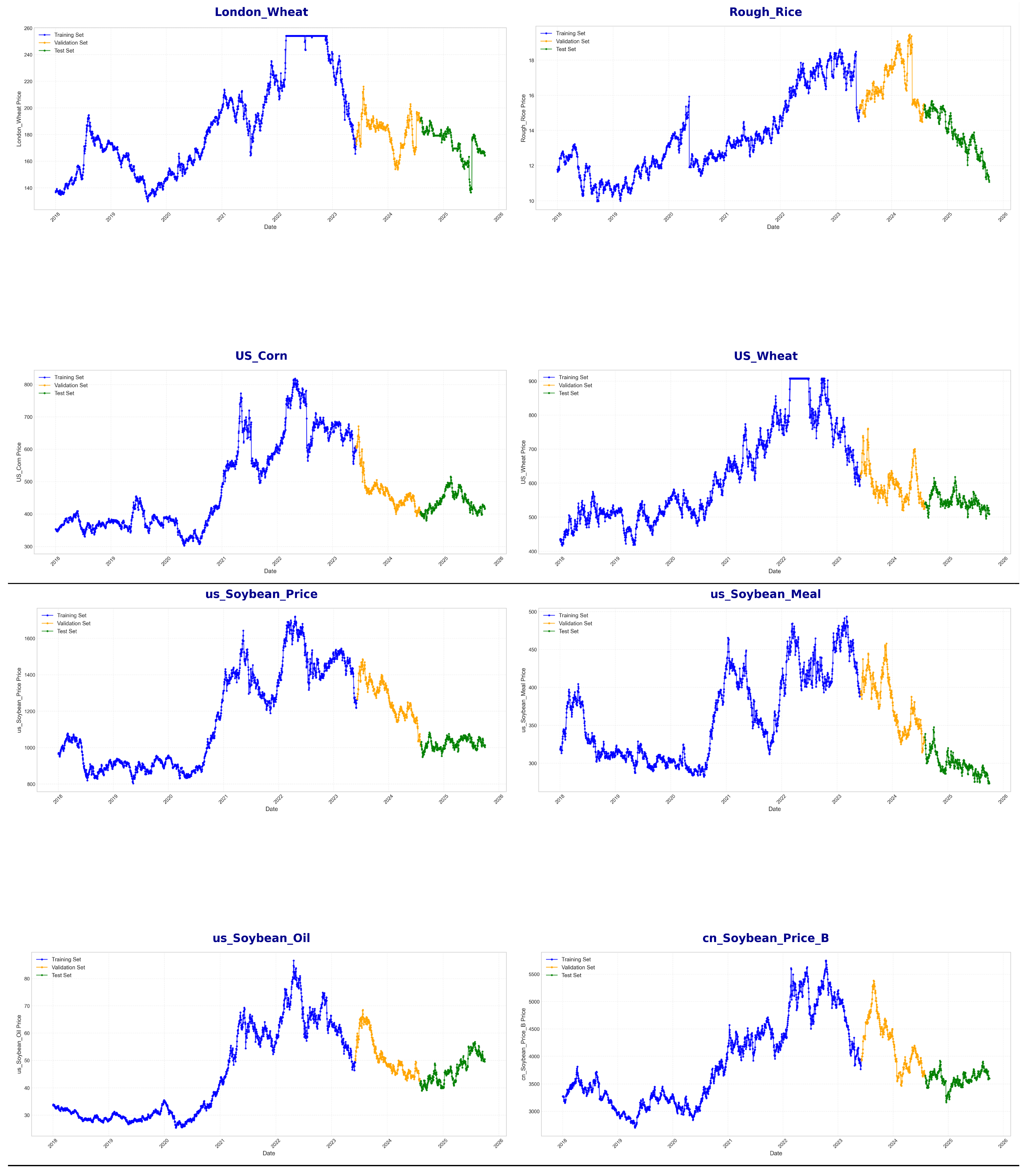
Figure A2.
Evolution of the Pareto front in the MCEORL ensemble optimization.
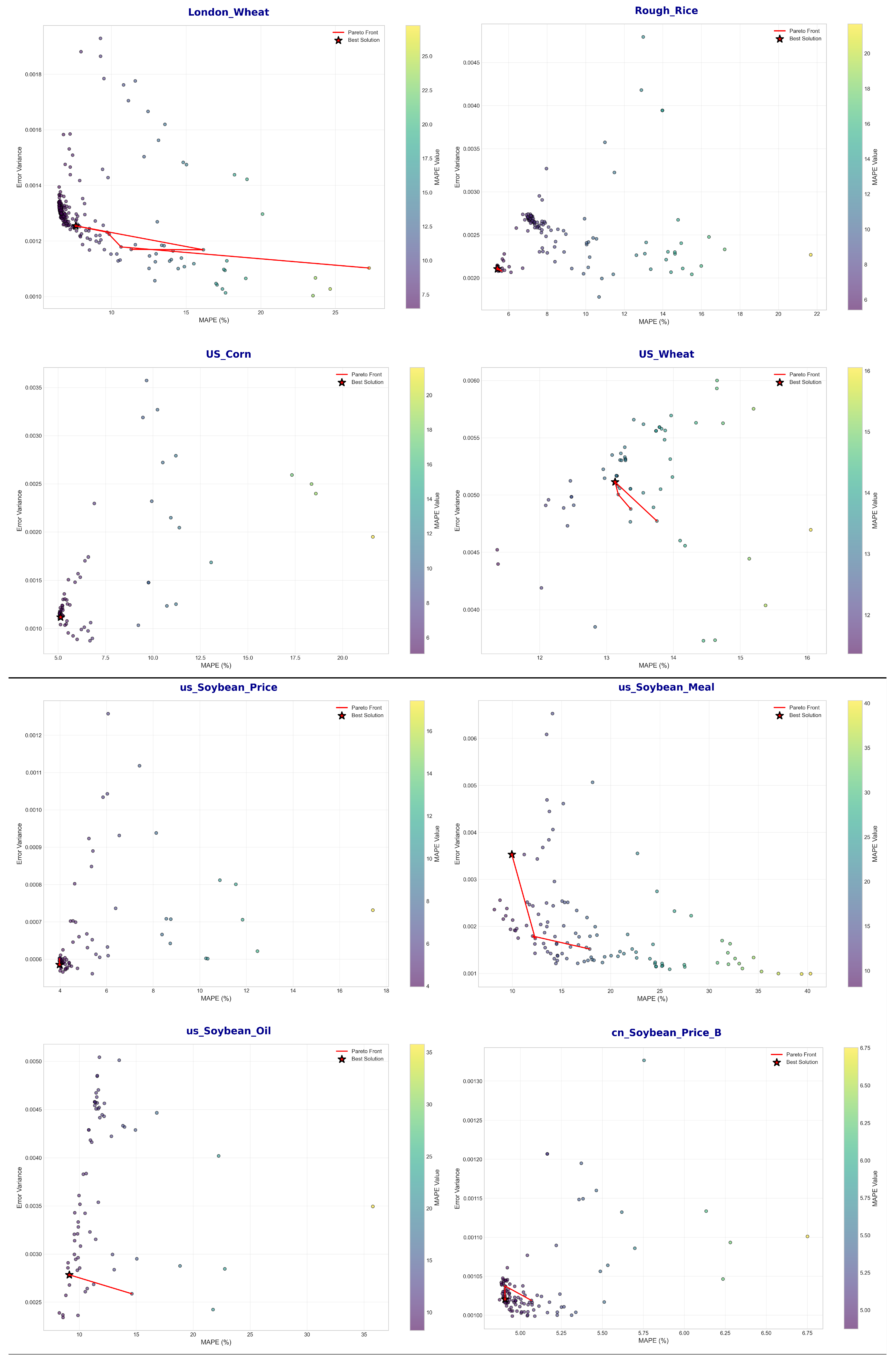
Figure A3.
SHAP-based feature importance analysis for agricultural commodities.
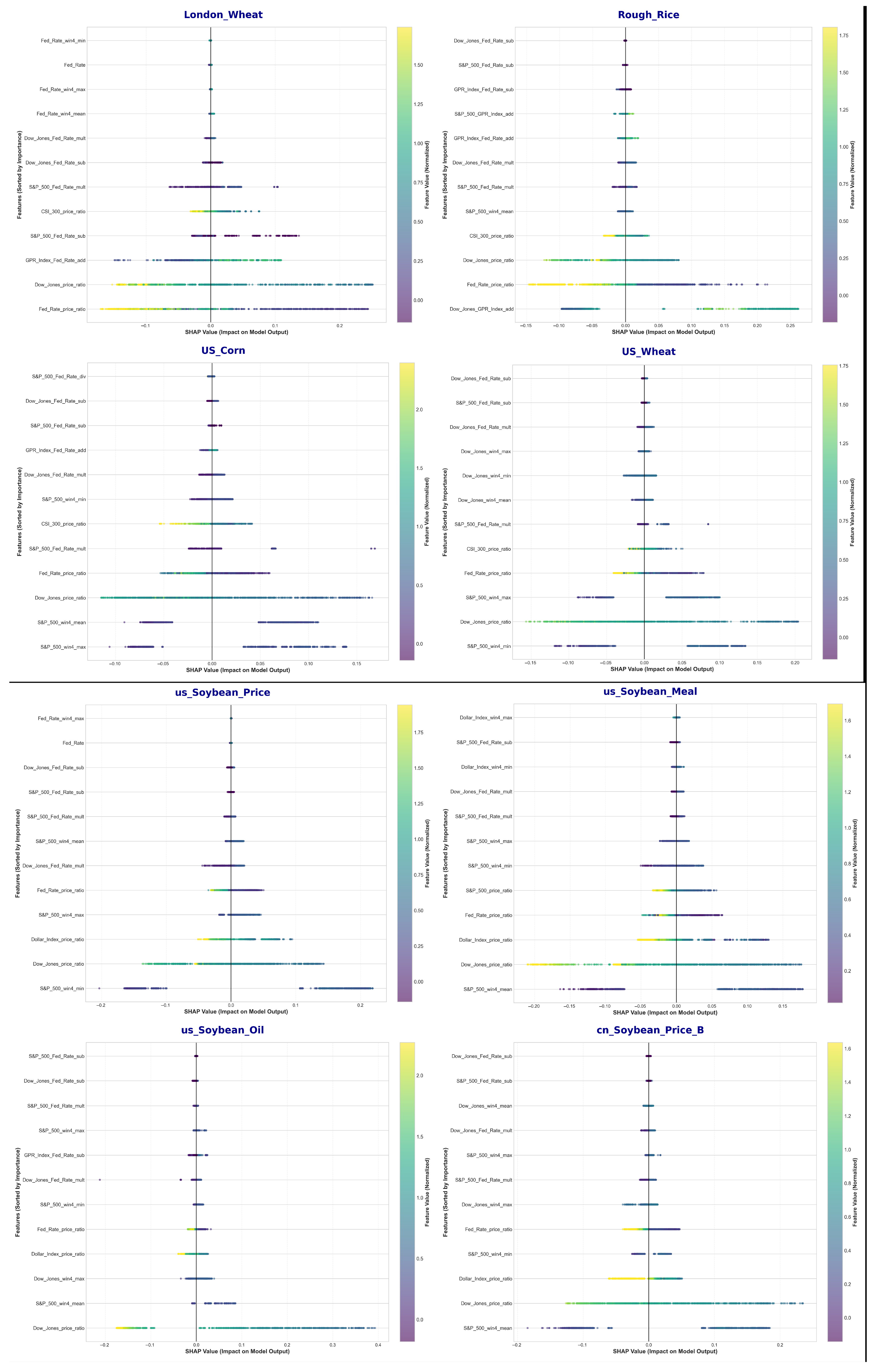
Table A1.
Top-3 base-model results by test-set MAPE across commodities.
Table A2.
Parameter configuration of the MCEORL reinforcement learning and chaotic evolution optimization algorithm.
Table A3.
Top-weighted forecasting models and ensemble weight allocation across commodities.
Table A4.
Sensitivity analysis of the minimum weight bound w on US Corn validation performance.
Table A5.
LIME local feature contribution results across commodities (Part A).
Table A6.
LIME local feature contribution results across commodities (Part B).
Table A7.
Summary of trading performance and strategy parameters across commodities.
Table A8.
Robustness-check results grouped by commodity.
Table A9.
Robustness checks: sub-period and weekly data performance (US Corn).
References
- Ahumada, H.; Cornejo, M. Forecasting food prices: The case of corn, soybeans and wheat. Int. J. Forecast. 2016, 32, 838–848. [Google Scholar] [CrossRef] [Scilit]
- Etienne, X.L.; Farhangdoost, S.; Hoffman, L.A.; Adam, B.D. Forecasting the U.S. season-average farm price of corn. J. Commod. Mark. 2023, 30, 100333. [Google Scholar] [CrossRef] [Scilit]
- Ling, L.; Zhang, D.; Chen, S.; Mugera, A.W. Can online search data improve pork price forecasting? J. Forecast. 2020, 39, 671–686. [Google Scholar] [CrossRef] [Scilit]
- Wang, J.; Wang, Z.; Li, X.; Zhou, H. Artificial bee colony-based combination approach to forecasting agricultural commodity prices. Int. J. Forecast. 2022, 38, 21–34. [Google Scholar] [CrossRef] [Scilit]
- Celik, B.A.; Celik, S. Hybrid forecasting of agricultural commodity prices: Integrating machine learning, time series, and stochastic simulation models. Borsa Istanb. Rev. 2025, 25, 1440–1462. [Google Scholar] [CrossRef] [Scilit]
- Fischer, T.; Krauss, C. Deep learning with long short-term memory networks for financial market predictions. Eur. J. Oper. Res. 2018, 270, 654–669. [Google Scholar] [CrossRef] [Scilit]
- Kim, T.Y.; Kim, H.Y. Forecasting stock prices with a feature fusion LSTM-CNN model using different representations of the same data. Expert Syst. Appl. 2019, 115, 157–167. [Google Scholar] [CrossRef] [Scilit]
- Sezer, O.B.; Ozbayoglu, A.M. Financial time series forecasting with deep learning: A systematic literature review. Appl. Soft Comput. 2020, 90, 106181. [Google Scholar] [CrossRef] [Scilit]
- Patel, J.; Shah, S.; Thakkar, P.; Kotecha, K. Predicting stock and stock price index using fusion of machine learning techniques. Expert Syst. Appl. 2015, 42, 2162–2172. [Google Scholar] [CrossRef] [Scilit]
- Ganaie, M.A.; Hu, M.; Malik, A.K.; Tanveer, M.; Suganthan, P.N. Ensemble deep learning: A review. Inf. Fusion 2021, 63, 153–165. [Google Scholar] [CrossRef] [Scilit]
- Ribeiro, M.T.; Singh, S.; Guestrin, C. Why should I trust you? Explaining the predictions of any classifier. In Proceedings of the 22nd ACM SIGKDD International Conference on Knowledge Discovery and Data Mining; Association for Computing Machinery: New York, NY, USA, 2016; pp. 1135–1144. [Google Scholar] [CrossRef] [Scilit]
- Lundberg, S.M.; Erion, G.; Chen, H. From local explanations to global understanding with explainable AI for trees. Nat. Mach. Intell. 2020, 2, 56–67. [Google Scholar] [CrossRef] [Scilit] [PubMed]
- Gramegna, A.; Giudici, P. SHAP and LIME: An Evaluation of Discriminative Power in Credit Risk. Front. Artif. Intell. 2021, 4, 752558. [Google Scholar] [CrossRef] [Scilit] [PubMed]
- Çelik, T.B.; İcan, O.; Bulut, E. Extending machine learning prediction capabilities by explainable AI in financial time series prediction. Appl. Soft Comput. 2023, 132, 109876. [Google Scholar] [CrossRef] [Scilit]
- Giudici, P.; Piergallini, A.; Recchioni, M.C.; Raffinetti, E. Explainable Artificial Intelligence methods for financial time series. Phys. A Stat. Mech. Its Appl. 2024, 655, 130176. [Google Scholar] [CrossRef] [Scilit]
- Hertel, M.; Pütz, S.; Mikut, R.; Hagenmeyer, V.; Schäfer, B. Explainable time-series forecasting with sampling-free SHAP for Transformers. Nat. Commun. 2026, 17, 4723. [Google Scholar] [CrossRef] [Scilit] [PubMed]
- Arsenault, P.D.; Wang, S.; Patenaude, J.M. A Survey of Explainable Artificial Intelligence (XAI) in Financial Time Series Forecasting. ACM Comput. Surv. 2025, 57, 265. [Google Scholar] [CrossRef] [Scilit]
- Chen, S.; Rogoff, K.; Rossi, B. Exchange rate volatility and agricultural commodity prices. Rev. Econ. Stud. 2010, 77, 735–754. [Google Scholar]
- Christoffersen, P.; Lunde, A.; Olesen, K.V. Factor Structure in Commodity Futures Return and Volatility. J. Financ. Quant. Anal. 2019, 54, 1083–1115. [Google Scholar] [CrossRef] [Scilit]
- Foglia, M.; Palomba, G.; Tedeschi, M. Disentangling the geopolitical risk and its effects on commodities: Evidence from a panel of G8 countries. Resour. Policy 2023, 85, 104056. [Google Scholar] [CrossRef] [Scilit]
- Nazlioglu, S. World oil and agricultural commodity prices: Evidence from nonlinear causality. Energy Policy 2011, 39, 2935–2943. [Google Scholar] [CrossRef] [Scilit]
- Frankel, J.A. The Effect of Monetary Policy on Real Commodity Prices. In Asset Prices and Monetary Policy; Campbell, J.Y., Ed.; University of Chicago Press: Chicago, IL, USA, 2008; pp. 291–327. [Google Scholar]
- Peng, H.; Long, F.; Ding, C. Feature selection based on mutual information: Criteria of max-dependency, max-relevance, and min-redundancy. IEEE Trans. Pattern Anal. Mach. Intell. 2005, 27, 1226–1238. [Google Scholar] [CrossRef] [Scilit] [PubMed]
- Lundberg, S.M.; Lee, S.I. A unified approach to interpreting model predictions. In Proceedings of the Advances in Neural Information Processing Systems; Curran Associates Inc.: Red Hook, NY, USA, 2017; Volume 30, pp. 1–10. [Google Scholar]
- Deb, K. Multi-Objective Optimization Using Evolutionary Algorithms; John Wiley & Sons: Hoboken, NJ, USA, 2001. [Google Scholar]
- Strogatz, S.H. Nonlinear Dynamics and Chaos: With Applications to Physics, Biology, Chemistry, and Engineering, 2nd ed.; CRC Press: Boca Raton, FL, USA, 2018. [Google Scholar] [CrossRef] [Scilit]
- Watkins, C.J.; Dayan, P. Q-learning. Mach. Learn. 1992, 8, 279–292. [Google Scholar] [CrossRef] [Scilit]
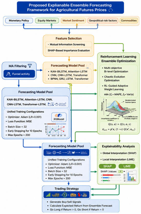
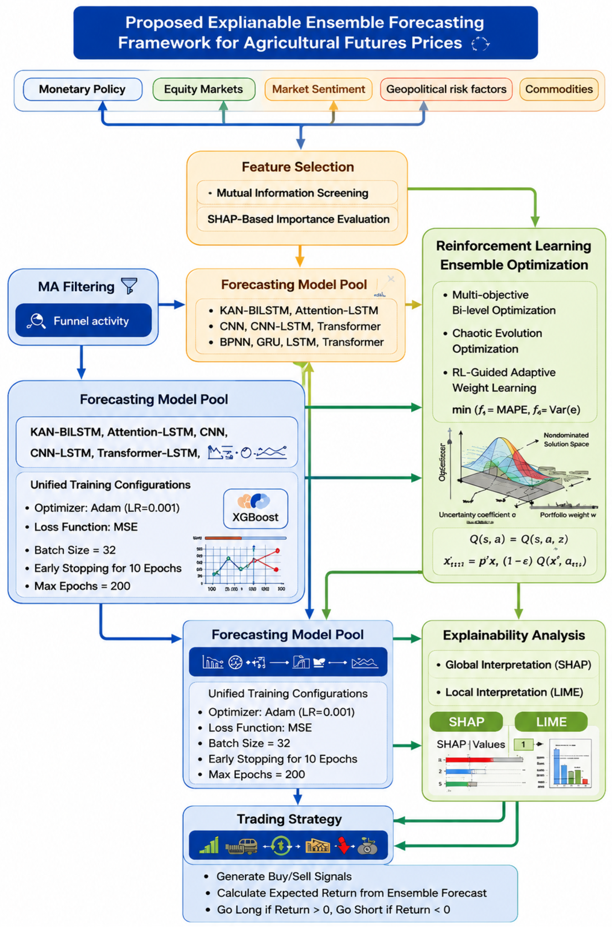
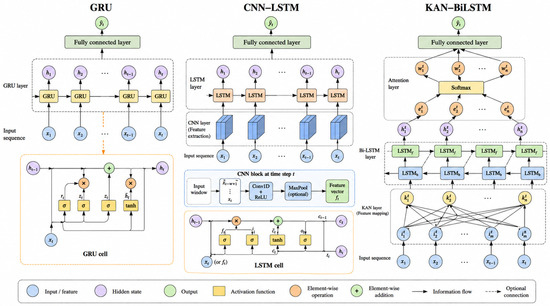
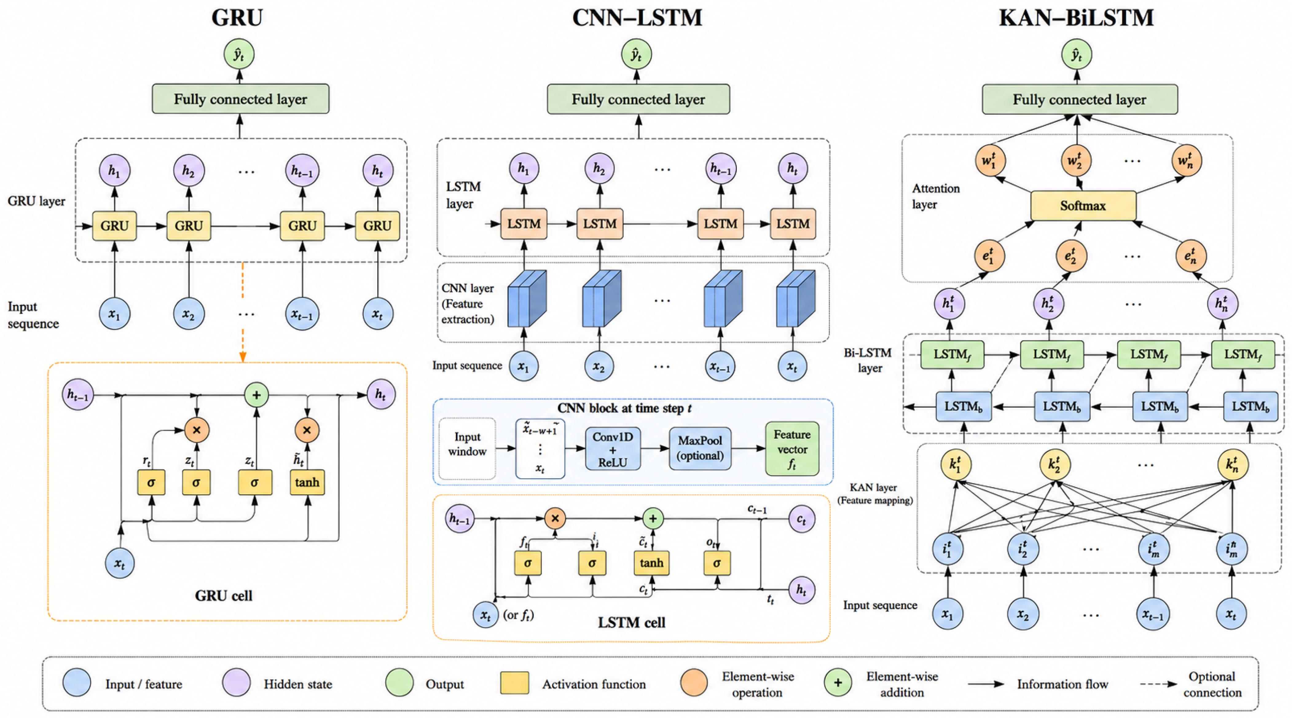
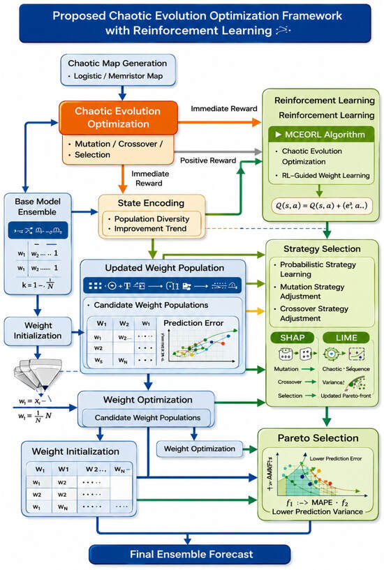
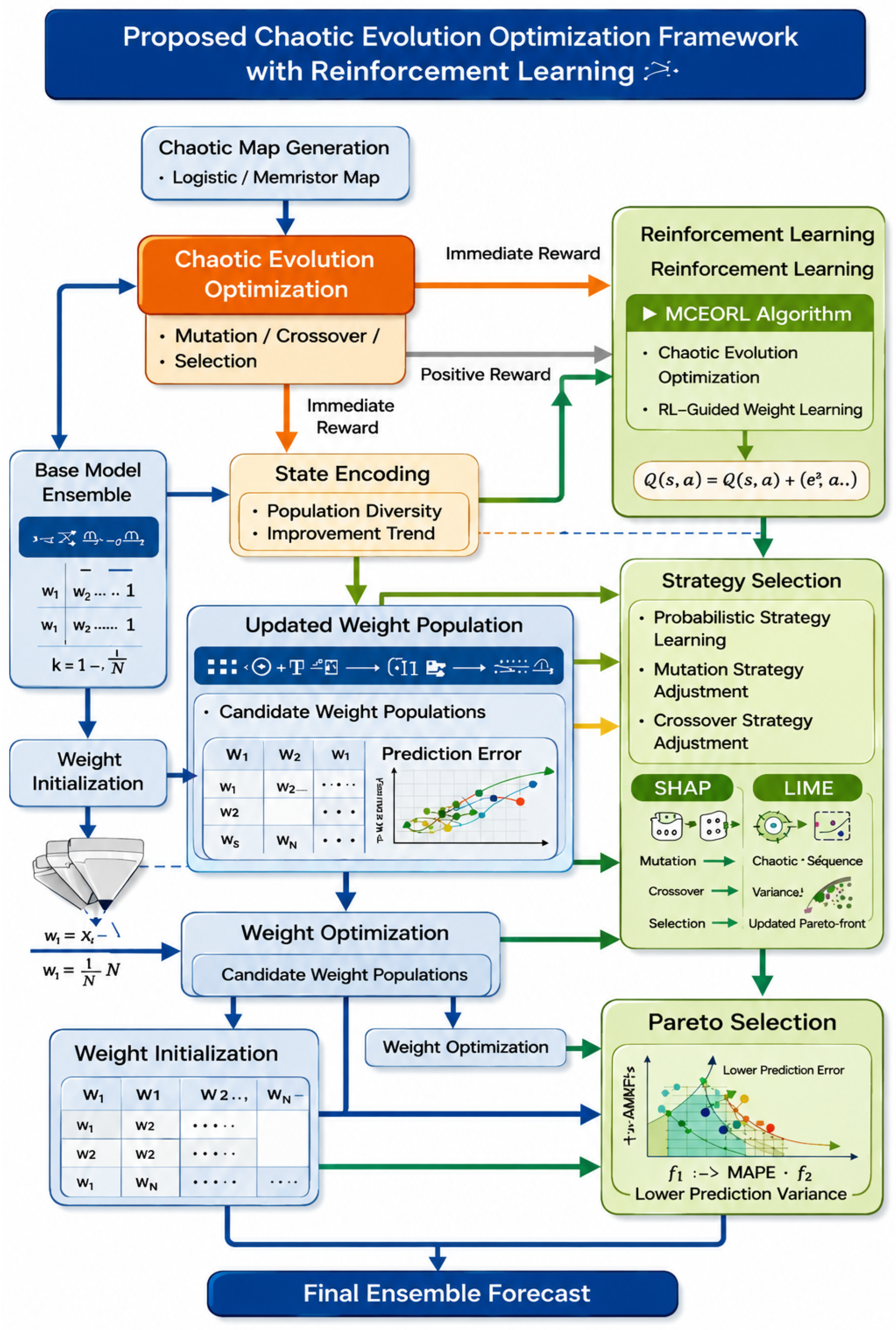
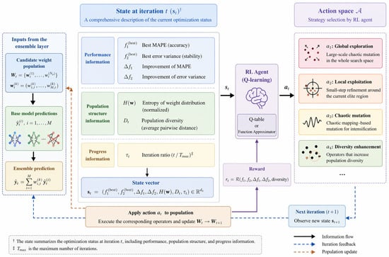
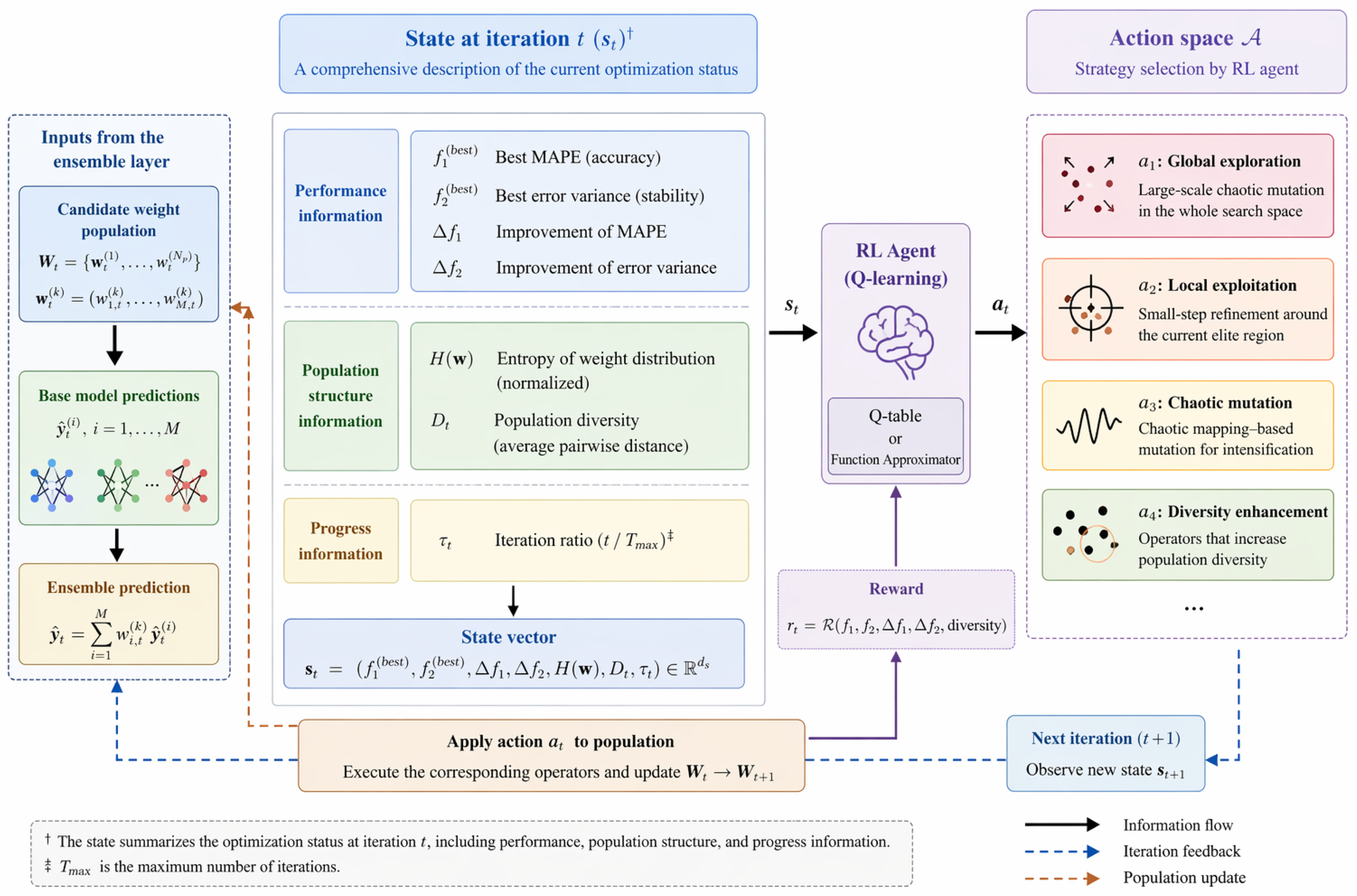
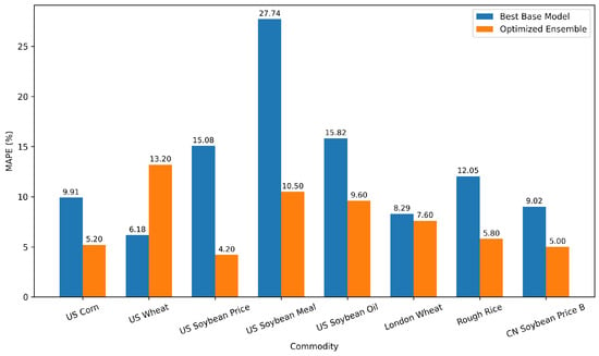
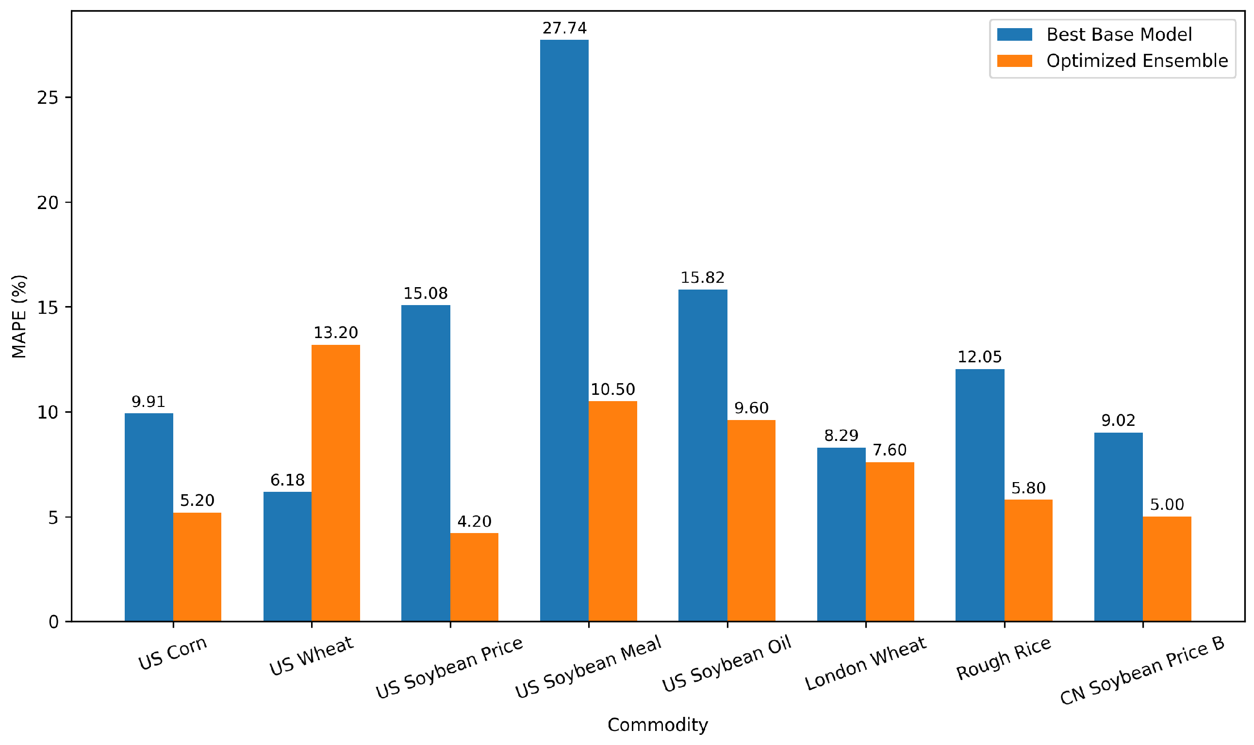
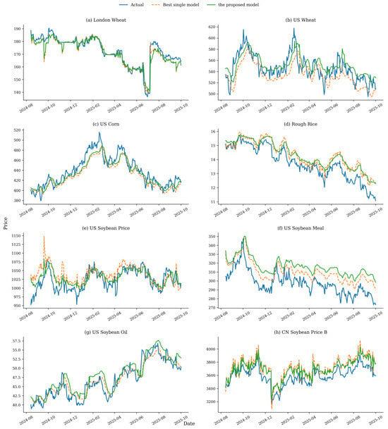
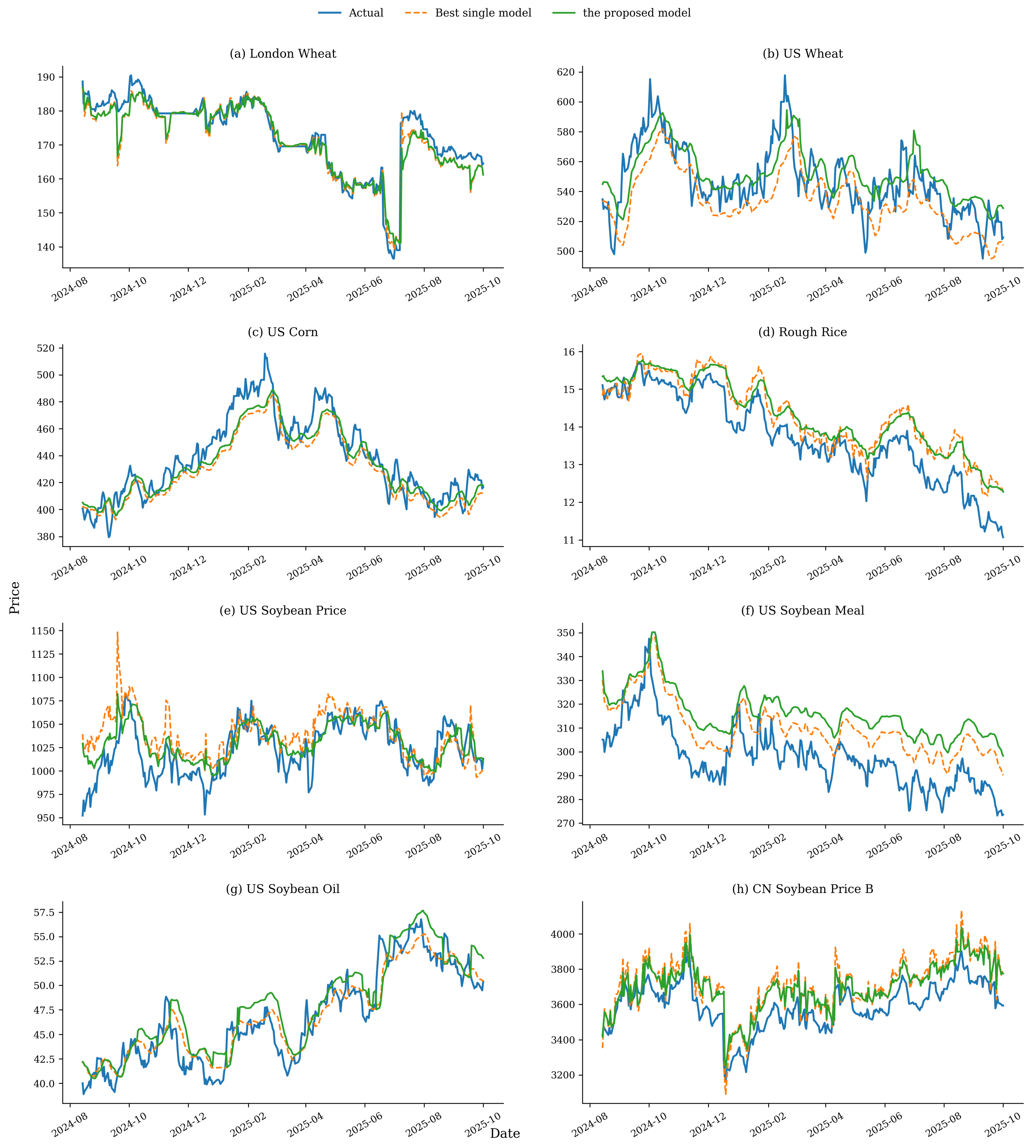
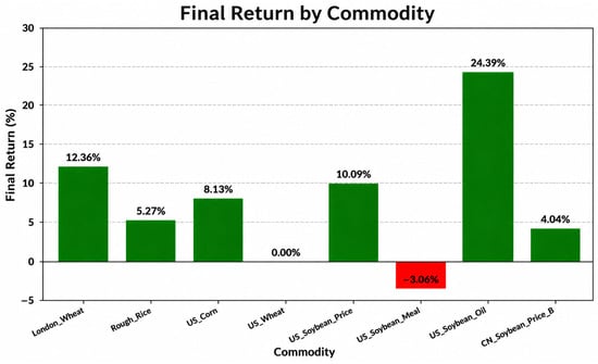
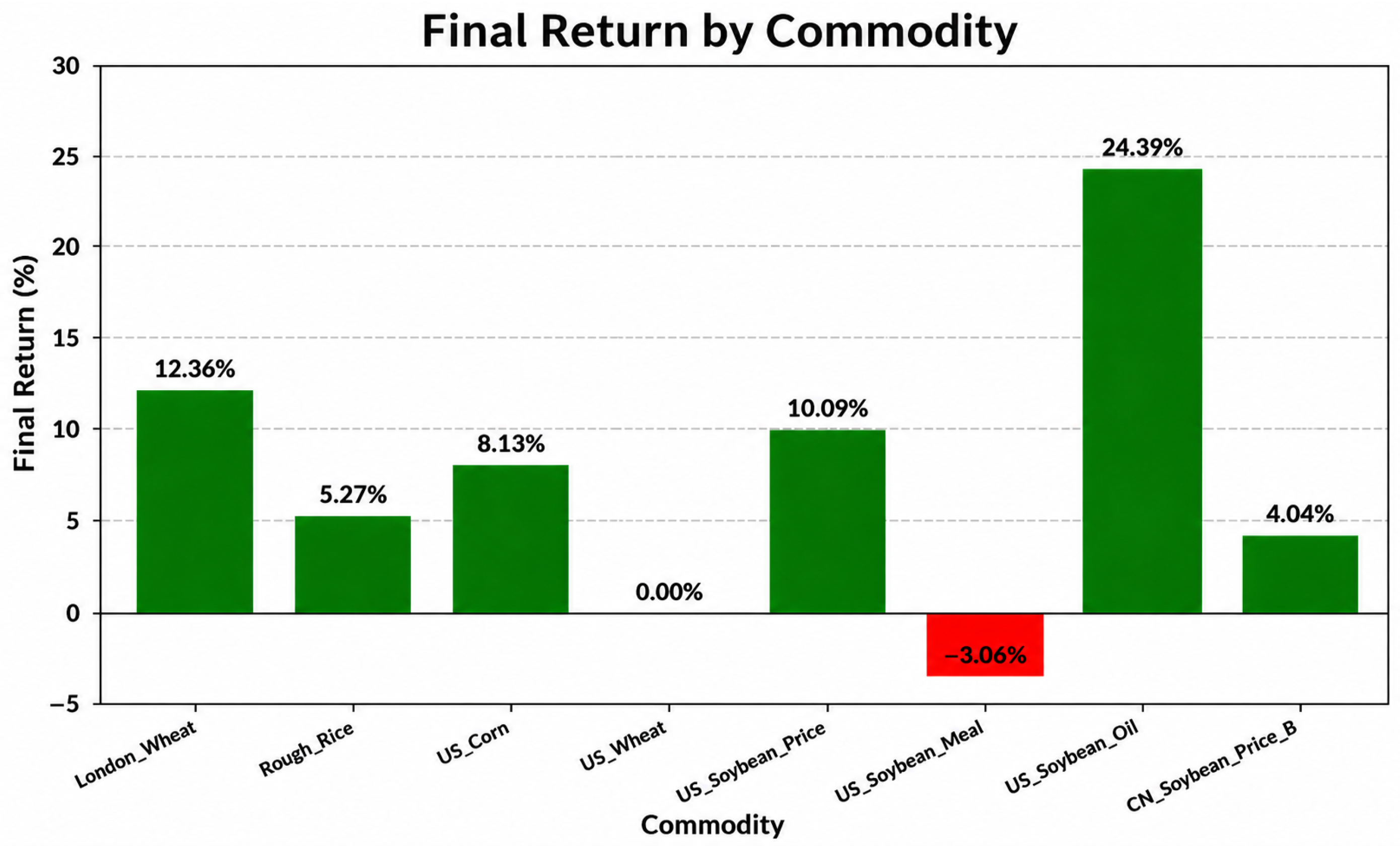
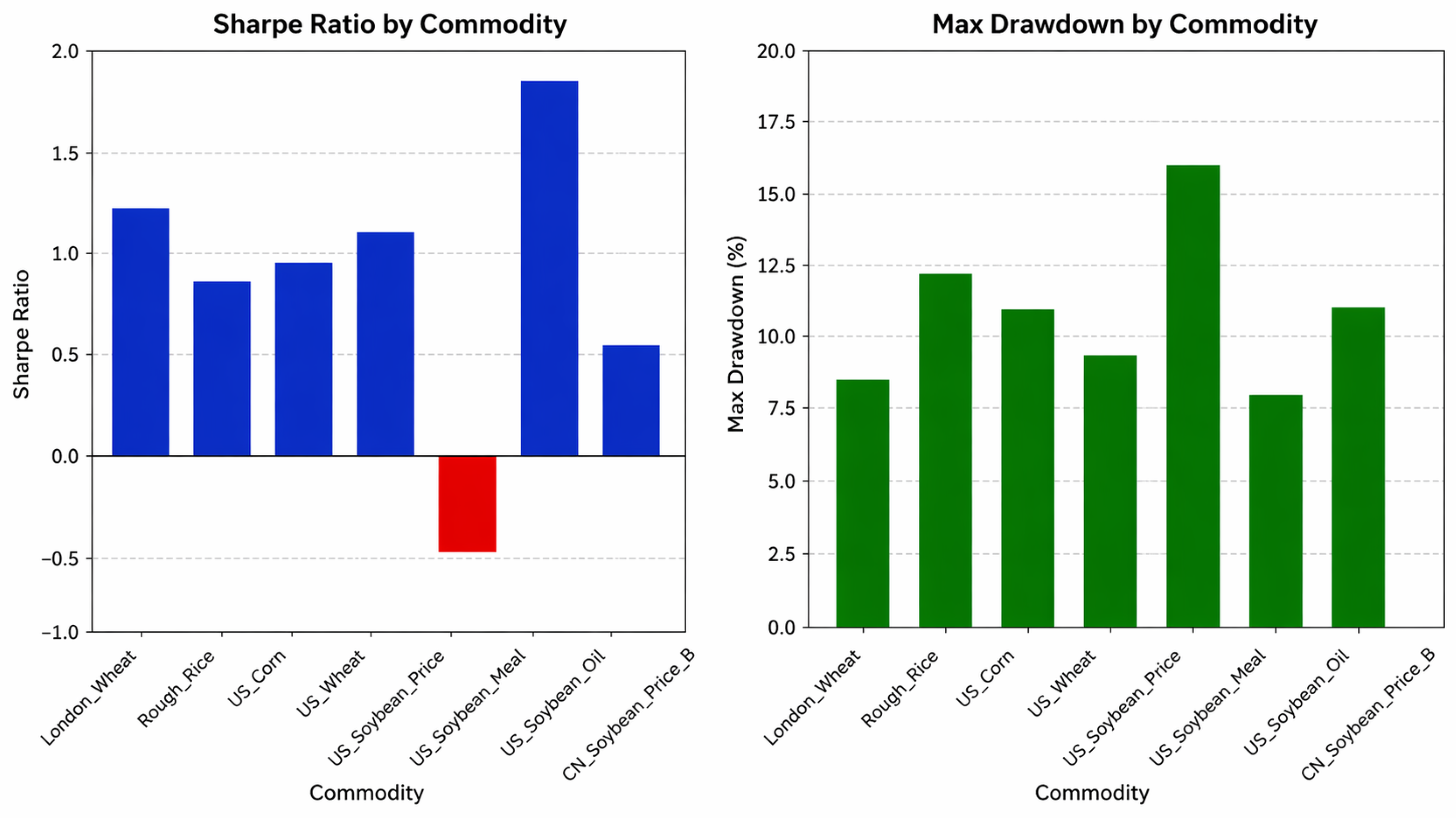

Disclaimer/Publisher’s Note: The statements, opinions and data contained in all publications are solely those of the individual author(s) and contributor(s) and not of MDPI and/or the editor(s). MDPI and/or the editor(s) disclaim responsibility for any injury to people or property resulting from any ideas, methods, instructions or products referred to in the content. |
© 2026 by the authors. Licensee MDPI, Basel, Switzerland. This article is an open access article distributed under the terms and conditions of the Creative Commons Attribution (CC BY) license.