Generalized Model Predictive Control Algorithm for a Five-Phase Induction Motor

Abstract

This paper proposes a Generalized Predictive Control (GPC) approach for the inner current-control loop of a multiphase induction motor drive. The method is based on a CARIMA model, which inherently provides integral action, allowing steady-state error rejection without the need for state or disturbance observers. In contrast to state-space Model Predictive Control (MPC), the proposed formulation enables the straightforward inclusion of system delays and yields an analytical solution when constraints are not considered, reducing computational complexity. Additionally, it is shown that the GPC is able to cope with modelling errors due to different dynamics at different operating points. The effectiveness of the approach is evaluated on a five-phase induction machine, showing competitive performance and improved robustness against modelling uncertainties.

1. Introduction

Predictive methods for variable speed drives have been the subject of research for several decades now [1,2]. In particular, predictive stator current control is based on an Indirect Field Oriented Control (IFOC) scheme [3]. IFOC uses a cascaded structure [4], where the outer loop is responsible for speed tracking and the inner loop for current control. Most proposals use this structure, where the inner loop is realized by predictive means.

The current trends consider two different sets of techniques: those that use explicit modulation and those that use implicit modulation. In the first category, the output of the predictive controller is a voltage that must be synthesized by the Voltage Source Inverter (VSI) using the Pulse Width Modulation technique (PWM) [5,6,7]. Since the output of the predictive controller is a continuous variable (i.e., not quantized), the technique is usually referred to as Continuous Control Set Model Predictive Control (CCSMPC).

Model Predictive Control (MPC) with implicit modulation is referred to as Finite State MPC and Finite Control Set MPC (FCSMPC) [8]. It does not need a PWM stage, providing an increase in control bandwidth [9]. The FCSMPC method has to face several challenges. First, the high number of switching configurations of the VSI, especially in the multiphase case, makes it computationally intensive [10,11]. Although this has recently been alleviated by the emergence of fast optimization methods [12,13,14], these methods work for only some cost functions [15]. Another challenge is the determination of the weighting factors that appear in the cost function. Again, recent work has been done regarding weighting factor elimination [16,17] so that tuning is not required. Other authors advocate for the selection of weighting factors as a means of retaining flexibility [18,19,20].

Another aspect is that the predictive horizon for FCSMPC has to be short because the optimization problem cannot be solved in closed form [21]. This, coupled with the finite computational power of any device, limits the predictive capability of the method. Finally, in most FCSMPC applications, nonidealities such as VSI delays and phase unbalancing are not considered in order to keep the model simple.

The main advantages of CCSMPC over traditional control stem from the characteristics of Model Predictive Control (MPC), namely the ability to incorporate models, consider different control objectives by means of a cost function, and get ahead of changes in reference. Another advantage is that it enables the use of recent advances in MPC. These are adequate to deal with challenges such as steady-state error rejection, inclusion of system delays, computational complexity reduction, and gain-scheduling strategies, among others. This is especially important if a complex model is needed, for instance to represent non-idealities in the system behaviour. Complex models are difficult to deal with in FCSMPC; however, in CCSMPC, the increased sampling period enables their use. An analytical expression for the optimization problem is often found for the unconstrained case, and quadratic programming is used otherwise [22]. This allows for sampling times around 200 ($\mu \mathrm{s}$) or lower, especially using fast optimization methods [23]. This has been established in [24], where digital control delay, pulse width modulation delay, inverter dead time, and measurement noise are considered. Regarding delays, please note that in FCSMPC the computation time produces a one-sample delay that must be compensated adequately [25]. This delay only appears in FCSMPC and must not be confused with VSI dead-time and with the delays inherent to pulse width modulation that appear in CCSMPC.

Regarding the techniques available for CCSMPC, it is worth considering Generalized Predictive Control (GPC). It is a member of the MPC family originally proposed by Clarke, Mohtadi, and Tuffs. The main difference between MPC strategies is the type of model used to predict the future evolution of the plant [26]. In the case of the GPC strategy, a discrete-time transfer function model of the plant is used [27,28]. Unlike conventional state-space CCS-MPC formulations, GPC is based on a discrete-time Controlled Auto-Regressive Integrated Moving-Average (CARIMA) input-output model to predict the future evolution of the controlled output. These models include the $\Delta$ operator, providing integral action, which allows offset-free tracking of constant references and rejection of constant disturbances. This is not possible for the standard nominal MPC derivation, where the disturbance polynomial is usually selected as 1. The $\Delta$ approach obviates the need to use strategies such as state observers or disturbance estimators to obtain offset-free set-point tracking [29].

In addition to the above, if the CARIMA models are obtained by identification, some of the non-idealities of the system will appear in the identification data and can potentially be incorporated into the model. Finally, the optimization problem can be formulated with constraints. When input, input-increment, or output constraints are considered, the linear prediction model and the quadratic cost function lead to a quadratic programming (QP) problem [30]. This problem can become unaffordable for typical Digital Signal Processors and sampling times used in drive control. However, saturation of the control signal can be considered.

Novelty and Contributions

The novelty of the paper deals with the way it handles a trade-off appearing in CCSMPC for drives. On the one hand, some existing CCSMPC schemes use complex models obtained from first principles. These hinder the real-time computation of the control signal. This produces an increase in the sampling period, which has a negative effect on performance.

On the other hand, reducing the model complexity can produce deviations from real behaviour. This is coupled with the fact that some non-idealities are difficult to model. As a result, some effects are typically neglected to avoid complicated modelling. This is the case of asymmetries that can be present in the VSI, in the stator windings, and in the rotor structure. Please note that model-based control can be sensitive to modelling errors, producing notable effects such as steady-state errors [30,31].

This trade-off between model complexity and sampling frequency is considered here by choosing a simple model structure whose parameters are obtained via identification. In this way, the most significant effects present in the identification data are also captured by the model without having to explicitly select them a priori. The advantage of using a CARIMA model is twofold: (i) simplicity, since only a discrete transfer function has to be identified using data from the real drive; and (ii) the formulation includes integral action, avoiding the use of disturbance estimators or integral controllers for offset-free tracking capabilities, which complicate the control strategy, as done in [24,32].

In addition, the computational requirements are low because of the use of the unconstrained explicit solution, whose gain matrix is computed offline. Thus, no matrix inversion or quadratic programming problem has to be solved in the real-time implementation. This makes the proposed approach affordable for modern Digital Signal Processors for the typical sampling times used in drive control.

As for the paper organization, the next section presents the controller structure based on a double loop. In Section 3, the experimental setup is presented and the identification test is explained. Following this, the proposal is assessed using the experimental platform. The paper ends with the conclusions section.

2. Controller Structure

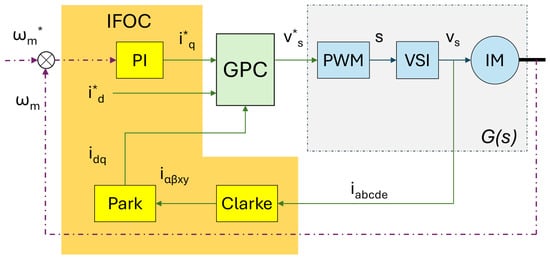
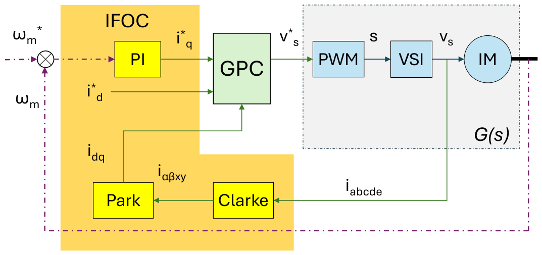
The proposed structure is a modification of the well-known Indirect Field Oriented Control (IFOC) scheme, as shown in Figure 1. The Clarke transform is used to convert stator phase currents ($i_{abcde}$) into $\alpha -\beta -x-y$ coordinates, which are useful for modelling purposes [33]. The Clarke transform is defined by a coordinate change matrix $T_p$ as

$$T_p=\left[\begin{array}{ccccc}1& cos\vartheta & cos2\vartheta & cos3\vartheta & cos4\vartheta \\ 0& sin\vartheta & sin2\vartheta & sin3\vartheta & sin4\vartheta \\ 1& cos2\vartheta & cos4\vartheta & cos\vartheta & cos3\vartheta \\ 0& sin2\vartheta & sin4\vartheta & sin\vartheta & sin3\vartheta \\ 1/2& 1/2& 1/2& 1/2& 1/2\end{array}\right]$$

(1)

where $\vartheta =2\pi /5$ for the five-phase IM.

Figure 1. Structure of the proposal.

The Park transform is used to convert the $\alpha -\beta -x-y$ coordinates to $d-q$ components. The Park transformation is provided by matrix D defined as

$$D=\left[\begin{array}{cc}cos\sigma & sin\sigma \\ -sin\sigma & cos\sigma \end{array}\right]$$

(2)

where the flux position $\sigma$ is obtained from the electrical frequency ${\omega }_e$ by means of $\sigma =\int {\omega }_{e}dt$. The $d-q$ decomposition allows the direct ($i_d$) and quadrature ($i_q$) current components to be treated independently. The direct component is the flux-producing current, and it is set to a constant (rated) value used to maintain the machine’s magnetic flux. The quadrature component is used to produce the torque required to achieve the reference mechanical speed (${\omega }^{*}$). This value is set by the outer loop. In most cases, a PI (Proportional-Integral Controller) is used for this loop [34]. The expression for the PI is

$$i_q^{*}\left(t\right)=k_p·e_{\omega }\left(t\right)+k_i{\int }_0^t{e}_{\omega }\left(\tau \right)d\tau$$

(3)

where $\omega$ is the measured speed and $e_{\omega }\left(t\right)={\omega }^{*}\left(t\right)-{\omega }^e\left(t\right)$ is the velocity error.

The tuning of the outer loop PI requires selecting a value for the Proportional Gain ($k_p$) and the Integral Gain ($k_i$). The first determines the stiffness of the motor. It is experimentally set by starting with a low value that is later increased until the motor tracks the speed step reference quickly without excessive overshoot. The integral gain is used to eliminate steady-state error. However, setting $k_i$ too high will cause low-frequency oscillations or instability [34].

The reference values in $d-q$ coordinates must be produced by the PWM. To do so, the inner control loop is used. In this proposal, the GPC block is used for this task. Recall that this loop is responsible for stator current generation. By doing so, the generated torque is manipulated and, hence, the angular speed of the motor (${\omega }_m$) can be controlled. The output of the GPC is the desired stator voltage $v_s^{*}$, which must be synthesized by the VSI block using a PWM strategy.

2.1. Methodology

In this paper, a black-box model is considered, including the PWM, VSI, and IM blocks. In the diagram in Figure 1, the black box is indicated as the transfer function $G\left(s\right)$. The transfer function considered links the reference voltage for the PWM ($V_s^{*}$) with the quadrature component of the stator currents ($i_q$).

$$G\left(s\right)={\displaystyle \frac{I_q\left(s\right)}{V_s^{*}\left(s\right)}},$$

(4)

where $I_q\left(s\right)$ is the Laplace transform of $i_q\left(t\right)$ and $V_s^{*}\left(s\right)$ is the Laplace transform of $v_s^{*}\left(t\right)$.

This way of proceeding has the advantage of allowing fast and robust GPC implementations to be used, with the potential to produce better results than other CCS approaches.

Obtaining an expression for $G\left(s\right)$ involves identification at some operating points of the motor. This will be shown in the experimental section. First, a model structure must be chosen. The structure must provide room to accommodate the observed behaviour and yet be simple enough for the predictive method to be run in real time. Considering this, a second-order model is chosen of the form

$$G\left(s\right)={\displaystyle \frac{Y\left(s\right)}{U\left(s\right)}}={\displaystyle \frac{(\frac{s}{c}+1)}{s^2+2\delta {\omega }_{n}s+{\omega }_n^2}}{k}_{est}{\omega }_n^2{e}^{-T_{d}s}$$

(5)

where s is the Laplace variable and the parameters are: $k_{est}$ (A/V) the static gain, c (${\mathrm{s}}^{-1}$) the zero, $\delta$ the damping factor, ${\omega }_n$ (rad/s) the natural frequency and $T_d$ (s) the delay.

This model structure can reproduce under-damped behaviour due to the second-order denominator. In the numerator, it contains a zero and a delay. The zero is used to shape the transient response of the real system, which is characterized by a strong initial response, as will be shown in the experimental part. Finally, the pure delay term $e^{-T_{d}s}$ is used to represent the PWM delay. Please note that this structure can be handled by the GPC algorithm, hence its adoption.

2.2. Induction Motor Model

The Five-phase Induction Motor (FIM) can be modeled from first principles equations that relate various electro-mechanical variables. For this application, the most important are the mechanical speed (${\omega }_m$), the stator current ($i_s$) and the stator voltage ($v_s$).

Considering a uniform stator-rotor air gap and sinusoidal magneto-motive force distribution, the following equation is found [24]

$${\displaystyle \frac{dx}{dt}}\left(t\right)=A_c\left({\omega }_r\left(t\right)\right)x\left(t\right)+B_{c}v\left(t\right)$$

(6)

The state vector (x) contains the $\alpha -\beta$ and $x-y$ stator currents and the $\alpha -\beta$ rotor currents as follows $x={(i_{s\alpha },i_{s\beta },i_{sx},i_{sy},i_{r\alpha },i_{r\beta })}^T$. The input variable is the stator voltage $v={(v_{s\alpha },v_{s\beta },v_{sx},v_{sy})}^T$. Matrices A and B depend on the rotor electric speed ${\omega }_r$ as follows.

$$A_c=\left[\begin{array}{cccccc}-a_{s2}& a_{m4}& 0& 0& a_{r4}& a_{l4}\\ -a_{m4}& -a_{s2}& 0& 0& -a_{l4}& a_{r4}\\ 0& 0& -a_{s3}& 0& 0& 0\\ 0& 0& 0& -a_{s3}& 0& 0\\ a_{s4}& -a_{m5}& 0& 0& -a_{r5}& -a_{l5}\\ a_{m5}& a_{s4}& 0& 0& a_{l5}& -a_{r5}\end{array}\right],B_c=\left[\begin{array}{cccc}{c}_2& 0& 0& 0\\ 0& c_2& 0& 0\\ 0& 0& c_3& 0\\ 0& 0& 0& c_3\\ -c_4& 0& 0& 0\\ 0& -c_4& 0& 0\end{array}\right]$$

(7)

The coefficients used are: $c_1=L_s{L}_r-L_m^2$, $c_2=L_r/c_1$, $c_3=1/L_{ls}$, $c_4=L_m/c_1$, $c_5=L_s{c}_1$, $a_{s2}=R_s{c}_2$, $a_{s3}=R_s{c}_3$, $a_{s4}=R_s{c}_4$, $a_{r4}=R_r{c}_4$, $a_{r5}=R_r{c}_5$, $a_{l4}=L_r{c}_4{\omega }_r$, $a_{l5}=L_r{c}_5{\omega }_r$, $a_{m4}=M{c}_4{\omega }_r$ and $a_{m5}=M{c}_5{\omega }_r$.

Stator voltage is achieved by using PWM on the VSI. In $\alpha -\beta -x-y$ coordinates, this results in the vector $v=\left(v_{s\alpha },v_{s\beta },v_{sx},v_{sy}\right)$, which can be expressed as $v=V_{DC}·S·T_M$, where $V_{DC}$ is the DC-link voltage, S is a vector containing the gating signals of the VSI, and $T_M=T·M$, with T being the connectivity matrix of the VSI and M a coordinate transformation matrix. Their product is found as:

$$T_M={\displaystyle \frac{2}{25}}\left[\begin{array}{ccccc}4& -1& -1& -1& -1\\ -1& 4& -1& -1& -1\\ -1& -1& 4& -1& -1\\ -1& -1& -1& 4& -1\\ -1& -1& -1& -1& 4\end{array}\right]·\left[\begin{array}{ccccc}1& cos\vartheta & cos2\vartheta & cos3\vartheta & cos4\vartheta \\ 0& sin\vartheta & sin2\vartheta & sin3\vartheta & sin4\vartheta \\ 1& cos2\vartheta & cos4\vartheta & cos\vartheta & cos3\vartheta \\ 0& sin2\vartheta & sin4\vartheta & sin\vartheta & sin3\vartheta \\ 1/2& 1/2& 1/2& 1/2& 1/2\end{array}\right]$$

(8)

where $\vartheta =2\pi /5$.

2.3. Generalized Model Predictive Control Strategy

In this section, the Generalized Predictive Control (GPC) algorithm is presented. In classical GPC, the plant is commonly represented by a Controlled Auto-Regressive Integrated Moving-Average model, usually referred to as a CARIMA model:

$$A\left(z^{-1}\right)y\left(k\right)=z^{-d}B\left(z^{-1}\right)u\left(k\right)+{\displaystyle \frac{C\left(z^{-1}\right)}{\Delta }}e\left(k\right)$$

(9)

where $e\left(k\right)$ is a zero-mean disturbance term and

$$\Delta =1-z^{-1}$$

(10)

is the difference operator. Defining

$$\tilde{A}\left(z^{-1}\right)=A\left(z^{-1}\right)\Delta ,$$

(11)

the CARIMA model can be expressed in incremental form as

$$\tilde{A}\left(z^{-1}\right)y\left(k\right)=z^{-d}B\left(z^{-1}\right)\Delta u\left(k\right).$$

(12)

To determine the future evolution of the output, a formulation that depends on future input values is required. The j-step-ahead prediction is obtained from the Diophantine equation:

$$1=E_j\left(z^{-1}\right)\tilde{A}\left(z^{-1}\right)+z^{-j}{F}_j\left(z^{-1}\right),$$

(13)

where $E_j\left(z^{-1}\right)$ and $F_j\left(z^{-1}\right)$ are polynomials depending on the prediction step j. Using this equation, the predicted output can be written as

$$\widehat{y}(k+j|k)=F_j\left(z^{-1}\right)y\left(k\right)+E_j\left(z^{-1}\right)B\left(z^{-1}\right)\Delta u(k+j-d).$$

(14)

The first term represents the free response, which depends only on past data, while the second term represents the forced response due to future control increments.

The predictions are collected over a prediction horizon $N_p$, while the future control increments are optimized over a control horizon $N_c$. Thus, the prediction model can be written in matrix form as

$$\widehat{\mathbf{Y}}=\mathbf{f}+\mathbf{G}\Delta \mathbf{U},$$

(15)

where

$$\widehat{\mathbf{Y}}=\left[\begin{array}{c}\widehat{y}(k+1|k)\\ \widehat{y}(k+2|k)\\ ⋮\\ \widehat{y}(k+N_p|k)\end{array}\right],\Delta \mathbf{U}=\left[\begin{array}{c}\Delta u\left(k\right)\\ \Delta u(k+1)\\ ⋮\\ \Delta u(k+N_c-1)\end{array}\right].$$

(16)

The variable $\mathbf{f}$ stands for the free response and $\mathbf{G}$ is the dynamic matrix relating future control increments to future output predictions:

$$\mathbf{G}=\left[\begin{array}{cccc}{g}_1& 0& \dots & 0\\ g_2& g_1& \dots & 0\\ ⋮& ⋮& \ddots & ⋮\\ g_{N_p}& g_{N_p-1}& \dots & g_{N_p-N_c+1}\end{array}\right].$$

(17)

The GPC control law is obtained by minimizing the quadratic criterion

$$J={\displaystyle \sum _{j=1}^{N_p}}{\delta }_j{\left[\widehat{y}(k+j|k)-w(k+j)\right]}^2+{\displaystyle \sum _{j=1}^{N_c}}{\lambda }_j{\left[\Delta u(k+j-1)\right]}^2,$$

(18)

where $w(k+j)$ is the future reference, ${\delta }_j\ge 0$ weights the tracking error, and ${\lambda }_j>0$ penalizes the control effort. When considering SISO models, the parameter ${\delta }_j$ is usually considered to be 1.

The constrained GPC problem can be written as

$$\begin{array}{cc}\hfill \underset{\Delta \mathbf{U}}{min}& {\displaystyle \frac{1}{2}}\Delta {\mathbf{U}}^T\mathbf{H}\Delta \mathbf{U}+{\mathbf{c}}^T\Delta \mathbf{U}\hfill \\ \hfill \mathrm{s}.\mathrm{t}.& \mathbf{M}\Delta \mathbf{U}\le \mathbf{b},\hfill \end{array}$$

(19)

where

$$\mathbf{H}=2\left({\mathbf{G}}^T\mathbf{G}+\lambda \mathbf{I}\right),\mathbf{c}=2{\mathbf{G}}^T\left(\mathbf{f}-\mathbf{W}\right).$$

(20)

The matrix $\mathbf{M}$ and the vector $\mathbf{b}$ collect the linear constraints imposed on the future control increments, the future control signal, or the predicted output. $\mathbf{W}$ is the vector of the future references to be reached along the prediction horizon.

If constraints are not explicitly considered, the minimization problem admits an analytical solution. In that case, the optimal sequence of future control increments is obtained as

$$\Delta {\mathbf{U}}^{★}={\left({\mathbf{G}}^T\mathbf{G}+\lambda \mathbf{I}\right)}^{-1}{\mathbf{G}}^T\left(\mathbf{W}-\mathbf{f}\right).$$

(21)

Therefore, for fixed horizons and weighting factor $\lambda$, the gain

$${\mathbf{K}}_{\mathrm{GPC}}={\left({\mathbf{G}}^T\mathbf{G}+\lambda \mathbf{I}\right)}^{-1}{\mathbf{G}}^T$$

(22)

can be computed offline, yielding the explicit unconstrained control law

$$\Delta {\mathbf{U}}^{★}={\mathbf{K}}_{\mathrm{GPC}}\left(\mathbf{W}-\mathbf{f}\right).$$

(23)

According to the receding horizon strategy, only the first element of $\Delta {\mathbf{U}}^{★}$ is applied to the plant. Then, the optimal input sequence is computed again every sampling time. The first element is defined as

$$\Delta u\left(k\right)=\left[\begin{array}{cccc}1& 0& \dots & 0\end{array}\right]\Delta {\mathbf{U}}^{★}\left(k\right).$$

(24)

Since the sampling time for control purposes is selected as 200 $\mu \mathrm{s}$, solving a linear QP in real time would be very demanding. In this paper, the explicit solution of Equation (23) is used. The constraints are taken into account by saturating the control signal as follows.

$$u\left(k\right)=\left\{\begin{array}{cc}{V}_{max},\hfill & \mathrm{if}{u}_{\mathrm{GPC}}\left(k\right)>V_{max},\hfill \\ V_{min},\hfill & \mathrm{if}{u}_{\mathrm{GPC}}\left(k\right)<V_{min},\hfill \\ u_{\mathrm{GPC}}\left(k\right),\hfill & \mathrm{otherwise}.\hfill \end{array}\right.$$

(25)

2.4. Discrete Transfer Function Model

This subsection presents the discrete-time model used in the GPC strategy. As shown in Table 1, the five-phase induction motor is a nonlinear system whose dynamics changes significantly depending on the operating point.

Table 1. Operating points used in the experimental identification procedure.

${\mathbf{V}}^{\mathbf{o}}$	${\mathbf{I}}^{\mathbf{o}}$	${\mathbf{k}}_{\mathbf{est}}$	c	$\mathit{\delta }$	${\mathit{\omega }}_{\mathit{n}}$	${\mathbf{T}}_{\mathbf{d}}$
(V)	(A)	(A/V)	(${\mathbf{s}}^{-\mathbf{1}}$)	(–)	(rad/s)	(ms)
40.0	0.0293	0.0018	6.5	0.98	95	0.2
100.0	0.1821	0.0041	5.4	0.90	85	0.2
160.0	0.4651	0.0063	4.8	0.89	73	0.2
220.0	0.8804	0.0084	4.4	0.86	68	0.2
280.0	1.4282	0.0106	4.1	0.81	63	0.2

In this paper, the future evolution of the current $I_q$ is predicted using a linear second-order transfer function. The parameters of this model are obtained by averaging the values identified at the operating points shown in Table 1.

The continuous-time transfer function used as nominal model is obtained from the identification phase using data from the real system. It features the structure of (5) with a set of parameters corresponding to the nominal operating point.

$$G\left(s\right)={\displaystyle \frac{0.00624·76.8^2\left(\frac{s}{5.04}+1\right)}{s^2+2·0.888·76.8s+76.8^2}}{e}^{-T_{d}s}.$$

(26)

Using the backward Euler approximation,

$$s\simeq {\displaystyle \frac{z-1}{z{T}_s}}={\displaystyle \frac{1-z^{-1}}{T_s}},$$

(27)

with $T_s=200\mu \mathrm{s}$, the discrete-time model obtained from (26) is

$$G\left(z^{-1}\right)=z^{-d}{\displaystyle \frac{0.00142284-0.00142141z^{-1}}{1-1.97299z^{-1}+0.973222z^{-2}}},$$

(28)

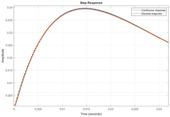
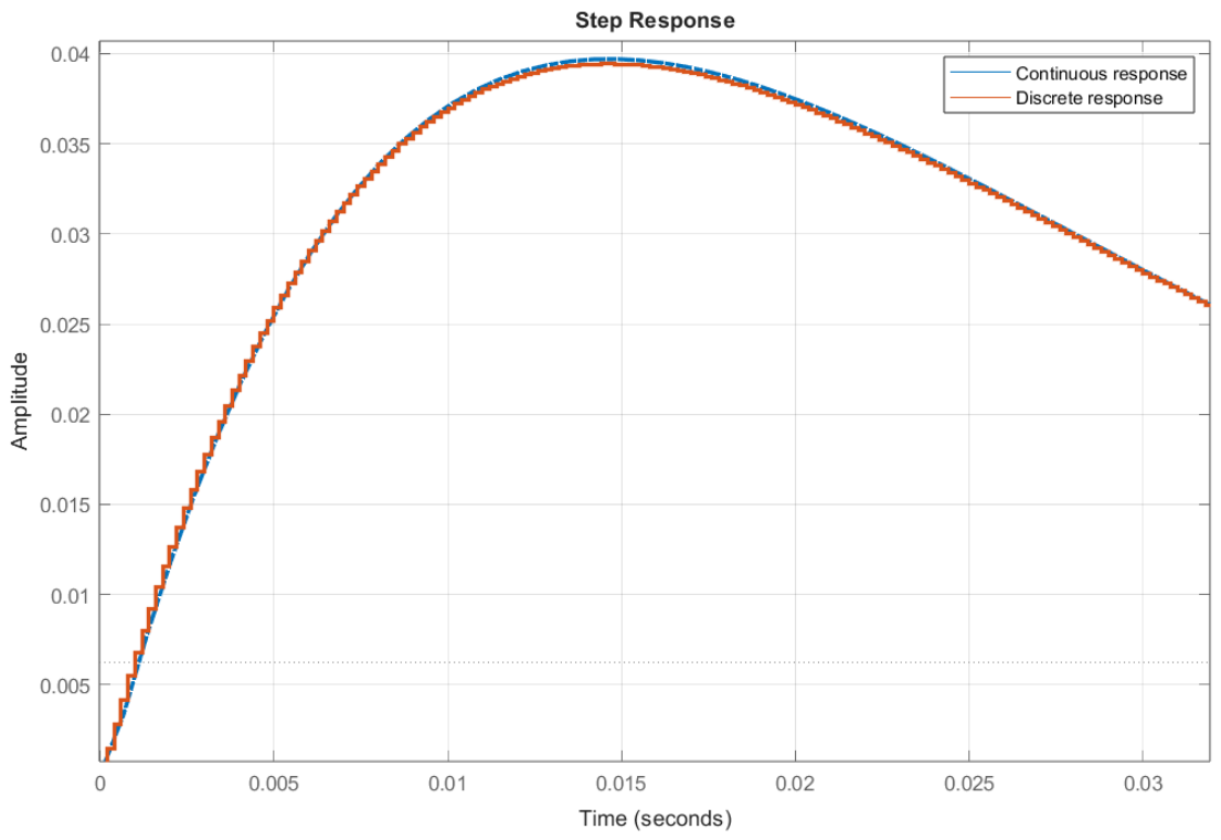
where d is the discrete-time delay associated with $T_d$. Figure 2 shows the comparison between the continuous and discrete transfer functions responses.

Figure 2. Comparison between continuous and discrete responses.

2.5. Control Algorithm

This subsection describes the final control algorithm implemented to control the motor angular speed. Every sampling period, the IFOC receives the error between the desired speed reference and the actual angular speed. Then a reference for the stator current $i_q^{*}$ is sent to the internal control loop. Then, the GPC control algorithm tracks the desired reference using the stator voltage as a control signal as shown in Figure 1.

The gain matrix ${\mathbf{K}}_{\mathrm{GPC}}$ is computed offline from the identified discrete-time model, the prediction horizon, the control horizon and the weighting factor. Therefore, no matrix inversion or QP problem is solved during real-time operation. The online computation is reduced to evaluating the free response, multiplying by the precomputed gain, applying the receding horizon strategy, and saturating the resulting voltage between $V_{min}$ and $V_{max}$.

The GPC current control algorithm with IFOC reference generation and voltage saturation is summarized in Algorithm 1.

Algorithm 1 Explicit GPC current-control algorithm with IFOC reference generation and voltage saturation

Require:  Discrete-time model $G\left(z^{-1}\right)$, prediction horizon $N_p$, control horizon $N_c$, weighting factor $\lambda$, voltage limits $V_{min}$, $V_{max}$, sampling time $T_s=200\mu \mathrm{s}$   1: Offline computation:   2: Build the prediction matrix $\mathbf{G}$ from the discrete-time model.   3: Compute the explicit GPC gain ${\mathbf{K}}_{\mathrm{GPC}}$ using (23)   4: Store ${\mathbf{K}}_{\mathrm{GPC}}$ for real-time implementation.   5: Online computation:   6: for each sampling instant k, with sampling time $T_s=200\mu \mathrm{s}$ do   7:  Measure the angular speed ${\omega }_m$ and compute the error ${\omega }_m^{*}-{\omega }_m$.   8:  Obtain the current reference $i^{★}\left(k\right)$ from IFOC.   9:  Build the future reference vector $\mathbf{W}\left(k\right)={[i^{★}(k+1),i^{★}(k+2),\dots ,i^{★}(k+N_p)]}^T$. 10:  Compute the free response vector $\mathbf{f}\left(k\right)$ from $f\left(k\right)=F_j\left(z^{-1}\right)y\left(k\right)$. 11:  Compute the optimal sequence $\Delta {\mathbf{U}}^{★}\left(k\right)={\mathbf{K}}_{\mathrm{GPC}}\left(\mathbf{W}\left(k\right)-\mathbf{f}\left(k\right)\right)$. 12:  Apply the receding horizon strategy defined in (24) to obtain $\Delta u\left(k\right)$. 13:  Compute the unconstrained GPC voltage $u_{\mathrm{GPC}}\left(k\right)=u(k-1)+\Delta u\left(k\right)$. 14:  Apply voltage saturation according to (25) to obtain $u\left(k\right)$. 15:  Apply $u\left(k\right)$ to the drive. 16: end for

2.6. Simulation Results

The subsection presents a simulation carried out using the linear model. The first step to tune the controller parameters is performed in a simulation environment. In this case, MATLAB 2024a software is used.

The tuning parameters of the GPC control strategy are the prediction horizon, $N_p$, the control horizon, $N_c$, and the parameter $\lambda$, which penalizes the control effort. There is no general rule to tune the controller parameters. However, some guidelines can be given. The prediction horizon should be long enough to cover the dominant transient of the identified model, including the effect of the zero of the transfer function. Since the system evolves in about 0.05 s, a prediction horizon of $N_p=250$ samples was selected. Since the sampling time is $T_s=200\mu \mathrm{s}$, this gives a prediction window of $0.05\mathrm{s}$. A shorter prediction horizon may not properly describe the evolution of the model from the initial transient to the region close to steady state. A larger horizon gives more weight to the steady-state part than to the transient part, which may worsen the dynamic response of the controller. Moreover, larger prediction horizons result in larger matrix sizes, which require more memory.

The control horizon was chosen as $N_c=100$. There is no general rule for selecting this parameter, as it mainly fixes the number of future control increments optimized by the controller. In practice, a value of $N_c$ close to one half of $N_p$ gave a good compromise between flexibility and controller aggressiveness.

Finally, the weighting factor $\lambda$ was first tuned in simulation and then adjusted on the real system. Lower values of $\lambda$ give faster responses, but also increase voltage activity and current ripple. In fact, small values of $\lambda$ may give rise to unstable behavior. Higher values produce smoother control signals, although the transient response becomes slower. A trade-off between stability, dynamic response and control effort is essential.

In order to show how the tuning parameters affect the closed loop system response, a sensitivity analysis has been carried out.

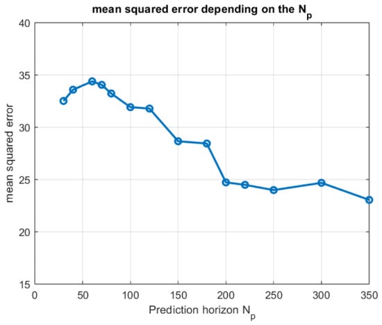
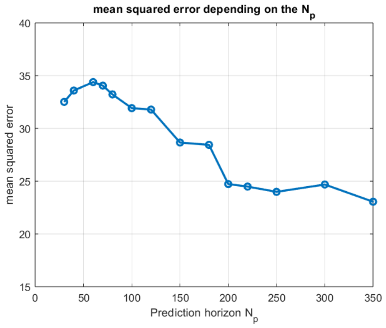
Figure 3 shows the evolution of the mean squared error as a function of the prediction horizon $N_p$, with the weighting factor $\lambda =0.003$. As can be observed, short prediction horizons lead to higher tracking errors, since the controller does not properly account for the dominant dynamics of the identified model. When $N_p$ is increased, the mean squared error decreases with a significant improvement for horizons above approximately $N_p=150$ samples. For larger values, the reduction becomes less pronounced, and the error tends to settle around a lower range. This behaviour supports the selection of a relatively long prediction horizon, such as $N_p=250$, as a suitable compromise between prediction capability and computational requirements.

Figure 3. Mean squared error as a function of the prediction horizon $N_p$, with $\lambda =0.003$.

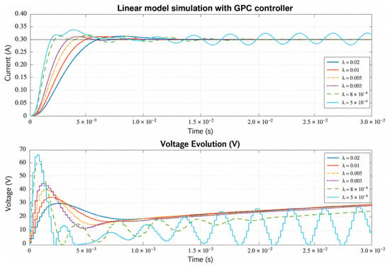
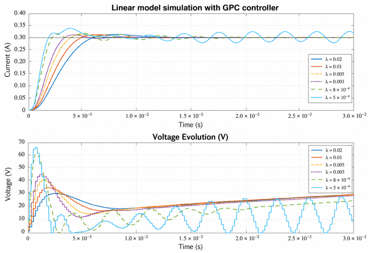
Figure 4 shows the closed-loop response obtained for different values of the weighting factor $\lambda$, with fixed horizons $N_p=250$ and $N_c=100$. As expected, lower values of $\lambda$ produce a more aggressive control action, leading to a faster current response but also to larger voltage variations and oscillations in steady state. In particular, very small values of $\lambda$ may produce an undesirable oscillatory behaviour. On the other hand, larger values of $\lambda$ smooth the voltage signal and reduce the oscillations, although the current response becomes slower. Therefore, $\lambda$ provides a direct tuning mechanism to balance dynamic response, voltage activity and steady-state ripple.

Figure 4. Sensitivity of the closed-loop response to the weighting factor $\lambda$, with $N_p=250$ and $N_c=100$.

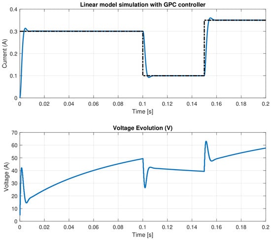
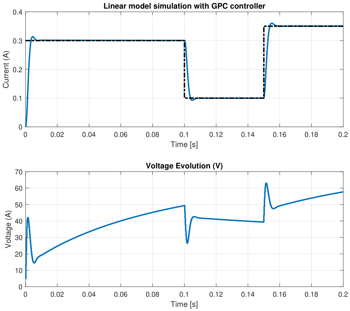
Figure 5 shows the closed-loop response obtained in simulation using the linear model and the proposed GPC controller. The current reference (dashed line) is properly tracked in all operating intervals, with a fast transient response, negligible steady-state error, and a rise time of about $0.005\mathrm{s}$. Small overshoots appear after the initial step and after the reference change at $t=0.15\mathrm{s}$, but the current rapidly converges to the desired value. The voltage evolution shows the expected sharp variations during transients and a smoother behavior once the current reaches its reference.

Figure 5. Simulation test.

3. Experimental Results

In this section, different experimental tests are provided. First, the laboratory system is described.

3.1. Laboratory Setup

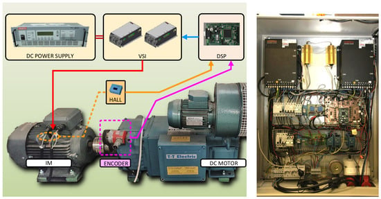
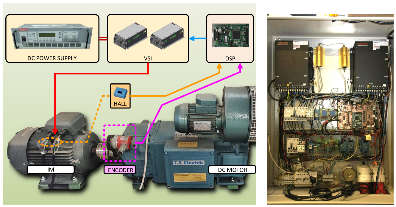
The laboratory system used for the experimental assessment of the proposal is composed of a five-phase induction machine, as shown in Figure 6. Each phase of the motor is electrically supplied by a VSI leg. The complete VSI is formed by two standard three-phase modules (SEMIKRON SKS 22F), of which only five legs are used. The VSI draws current from a 300 V DC power supply. The control algorithm runs in real time on a TMS320F28335 Digital Signal Processor (DSP). To this end, the DSP uses Hall-effect sensors (LH25-NP) to measure the stator phase currents.

Figure 6. Photographs of the elements composing the experimental setup (left) and of the electrical and control cabinet (right).

In addition to the IM, a co-axial direct current motor is used to provide an opposing torque, emulating a mechanical load connected to the IM. The laboratory setup parameters are provided in Table 2.

Table 2. Parameters of the induction motor.

Parameter	Value	Variable	Limit
Stator resistance, $R_s$	12.85 $\Omega$	Voltage limit $V_{DC}$	300 V
Rotor resistance, $R_r$	4.80 $\Omega$	Current limit, $I_{VSI}$	2.5 A
Stator inductance, $L_{ls}$	79.93 mH	Rated d-current, $I_{sd}^n$	0.9 A
Rotor inductance, $L_{lr}$	79.93 mH	Maximum torque, $T_{max}$	8.13 N m
Mutual inductance, $L_m$	681.7 mH
Rotational inertia, $J_m$	0.02 kg ${\mathrm{m}}^2$
Friction, $B_m$	0.0118 Nms/rad
Pole pairs, P	3

3.2. Experimental Identification

The block composed of the IM, VSI, and PWM has been modelled as a series of transfer functions, each for a different operating point. For each operating point, various step tests have been applied. Figure 7 shows the trajectories of the input ($v_s^{*}$) and output ($i_q$) for two of said tests. It is important to note that the behavior of the output changes with the operating point, represented in this case by the value of the voltages used. This can be observed in Figure 7, where the overshoot and static gain for the two tests are clearly visible.

Figure 7. Step tests for two operating points characterized by low voltages (left) and medium voltages (right).

From these trajectories, the identification procedure yields a transfer function. The order has been chosen as two in the denominator and one in the numerator, following Occam’s principle of economy.

As a first step, the input and output variables must use incremental values found as

$$u\left(t\right)=v_s^{*}\left(t\right)-V^o,y\left(t\right)=i_q\left(t\right)-I^o$$

(29)

where $V^o$ is the operating-point base value for the input variable and $I^o$ is the operating-point base value for the output variable. The set of all operating points can be found in Table 1.

The transfer function representing the IM, VSI, and PWM blocks has the form given in (5). This particular structure has been selected as the simplest one that can accommodate the observed behavior, characterized by a delay after which a fast initial response is seen. The response shows a large overshoot followed by an overdamped descent to the final value, as can be seen in the waveforms of Figure 7. The terms included in the transfer function of Equation (5) are the smallest set capable of reproducing the observed behavior.

The identification procedure uses the experimental data and a least mean squares algorithm to produce the values of the parameters for each operating point. The values are shown in Table 1.

3.3. Experimental Steady State Results

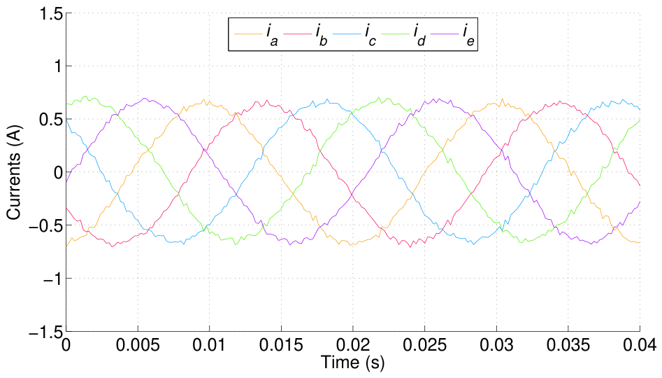
This first test aims at characterizing the stator current quality based on the observed waveforms. Figure 8 shows the waveforms of the phase stator currents. The results are in accordance with CCSMPC methods where modulation is carried out with a PWM. For the experiments a carrier frequency of 10 kHz has been used. This value is commonly found in IGBT based converters.

Figure 8. Waveforms of phase currents.

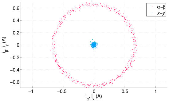
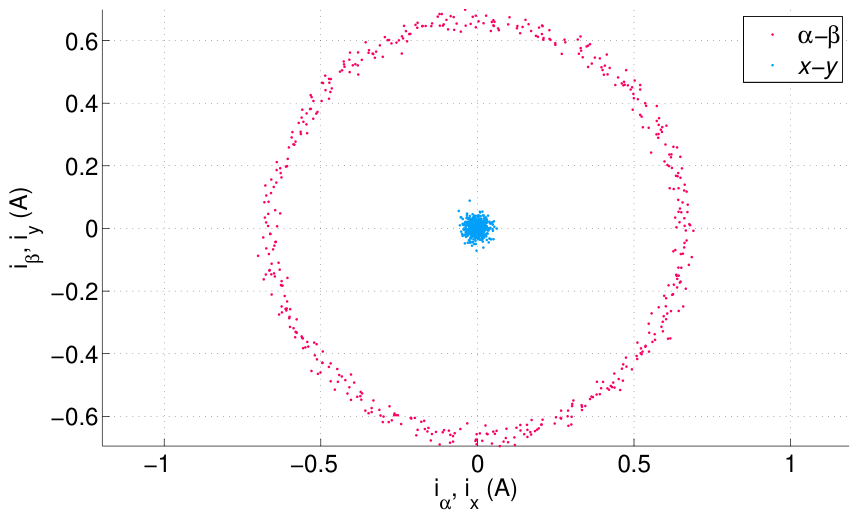
The hodogram of $\alpha -\beta$ and $x-y$ components is presented in Figure 9. In this way it is possible to check the precision of the $\alpha -\beta$ tracking and the $x-y$ content.

Figure 9. Hodogram of $\alpha -\beta$ and $x-y$ components.

3.4. Experimental Step Tests

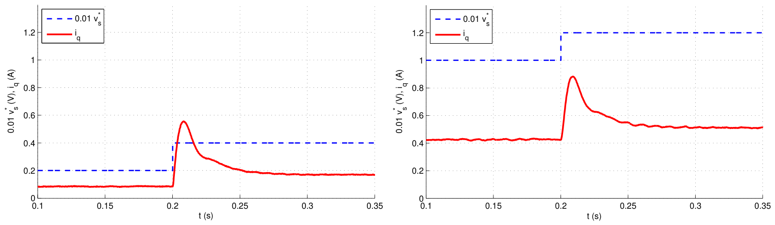
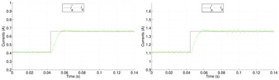
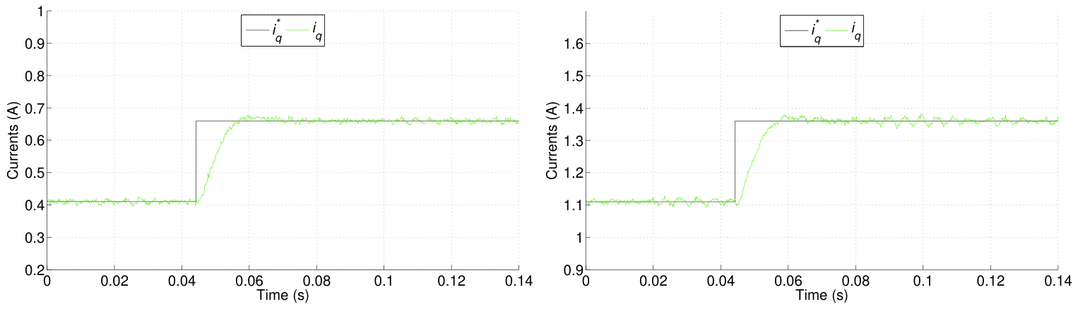
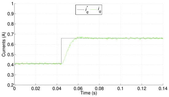
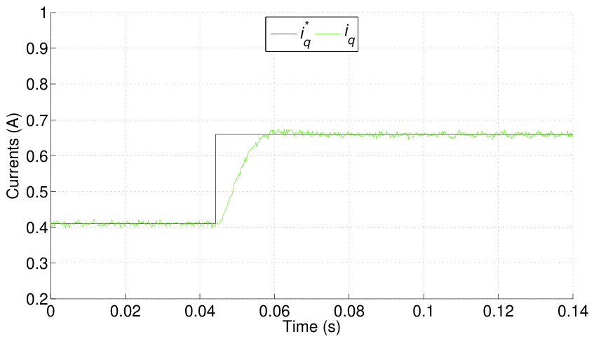
Transient tests are now performed with steps in the IM load. These are introduced by the co-axial DC machine of the experimental setup. Figure 10 presents the results using the $\alpha -\beta$ coordinates. The step is introduced at the time indicated by the vertical dashed line.

Figure 10. Results of the proposed GPC method for two step tests. Note the different span for the vertical axis on (left) and (right).

For these experiments the parameters of the GPC are $N_p=250$ (samples), $N_c=120$ (samples), and $\lambda =0.023$. The same tuning is used for both tests.

A different value of $\lambda$ has been used in a test to assess its influence on the results. The $i_q$ waveform is presented in Figure 11.

Figure 11. Results of the proposed GPC method for a higher value of the parameter $\lambda$.

3.5. Comparison with a FCSMPC

A comparison with an FCSMPC method is now presented. In the tests, the tuning of the outer loop PI is kept the same to provide a fair comparison. The figures of merit considered for the comparison are stator current ripple, percentage overshoot, rise time, and Average Switching Frequency (ASF). The latter is needed since FCSMPC does not provide a constant switching frequency, unlike CCSMPC approaches. As a result, one must count the number of switch changes at the VSI ($\Delta S\left(k\right)$) at each sampling period k and take an average. Similarly, for the current ripple, the instantaneous control error $e_{\alpha \beta xy}$ is measured and used to compute the root mean square value. The current ripple (R) and ASF are computed as follows

$$\begin{array}{ccc}\hfill R& =& \sqrt{{\displaystyle \frac{1}{(k_2-k_1+1)}}\sum _{k=k_1}^{k_2}{e}_{\alpha \beta xy}^2\left(k\right)}\hfill \end{array}$$

(30)

$$\begin{array}{ccc}\hfill ASF& =& {\displaystyle \frac{1/(5·2)}{t\left(k_2\right)-t\left(k_1\right)}}{\displaystyle \sum _{k=k_1}^{k_2}}\Delta S\left(k\right)\hfill \end{array}$$

(31)

In the previous expressions, the temporal span used to provide the mean values is defined by $k_1$ and $k_2$. These are defined so that they contain a couple of fundamental cycles, so $k_2=k_1+4\pi /\left({\omega }_e{T}_s\right)$, where ${\omega }_e$ is the electrical frequency and $T_s$ is the sampling period.

The results of the comparison can be seen in Table 3, where the figures of merit for the proposal and for an FCSMPC method are presented in different operating regimes. The regimes are characterized by speed and load. It can be seen that, in terms of electrical variables, the proposal outperforms FCSMPC. In terms of mechanical variables, the effect of the outer loop PI is dominant, and so both approaches are very similar.

Table 3. Figures of merit for the proposal and for a FCSMPC in different operating regimes characterized by speed and load.

Speed	Load	Ctrl.	Ripple	Overshoot	Rise Time	ASF
(%)	(%)		(mA)	(%)	(s)	(kHz)
25	25	FCS	102	5.21	0.012	6.2
25	25	Prop.	98	5.17	0.011	10
75	40	FCS	167	5.78	0.012	9.6
75	40	Prop	151	5.75	0.012	10
75	80	FCS	220	5.86	0.014	9.1
75	80	Prop	199	5.81	0.013	10
100	100	FCS	312	6.12	0.017	8.6
100	100	Prop	290	6.12	0.017	10

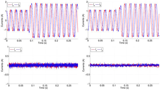
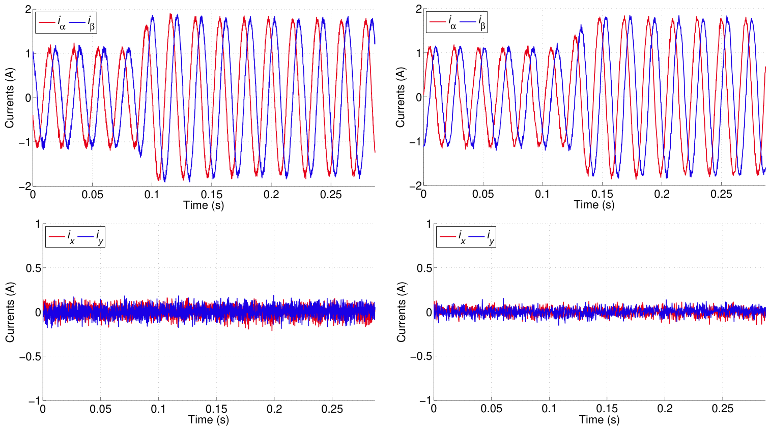
In addition to Table 3, Figure 12 presents the stator currents in the $\alpha -\beta$ and $x-y$ subspaces for a load step test. The current ripple is clearly visible, being more noticeable for the FCSMPC, especially in terms of $x-y$ content.

Figure 12. Comparison of the GPC method (right) with a FCSMPC (left) in terms of $\alpha -\beta$ tracking (upper row) and $x-y$ regulation (bottom row).

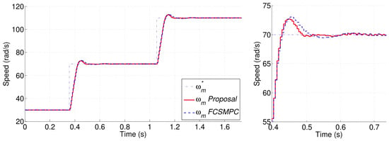
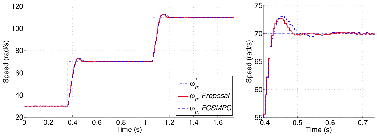
So far, the comparison has focused on electrical variables. This makes sense, as both controllers, the proposal and FCSMPC, are responsible for the inner loop for stator current control. It is interesting, however, to see how they perform in terms of drive speed control. Please bear in mind that this outer loop is largely determined by the outer PI controller. The tuning for this controller has been kept the same for the proposal and for FCSMPC in order to provide a fair comparison. Nevertheless, the torque-producing capability of both methods is not the same, and this is noticeable in the mechanical speed trajectories. This can be observed in Figure 13, where the mechanical speed reference is shown along the speed trajectories. Both controllers perform as expected for this kind of system. The overshoot is less than 9 % in both cases, and the rise time is very similar. Please note also that saturation in the control signal does contribute to the similarity of the results for both controllers.

Figure 13. Comparison of the proposal and a FCSMPC controller for a speed step test (left). A zoomed out view of the first step is presented on the (right) side.

Continuing with the comparison, the FCSMPC method is notorious for requiring high computing power. Table 4 provides a comparison of the execution times for FCSMPC and for the proposal. It can be seen that the proposal provides a substantial reduction in execution time thanks to the fact that it does not require the exhaustive optimization phase of FCSMPC.

Table 4. Execution times for the algorithms.

Task	FCSMPC	Proposal
	(μs)	(μs)
outer loop PI	1.80	1.80
control computation	25.80	4.30
A/D conversion	2.14	2.14
data logging	7.15	7.15
Total	36.91	15.39

3.6. Discussion

The results obtained by the proposed GPC show its ability to perform adequate control of the induction machine. The current quality is mainly determined by the PWM used to synthesize the stator voltage. In this regard, the proposal attains similar results to other CCSMPC methods. However, in transient tests, the proposal is able to react to fast changes in load with a very low overshoot, as can be seen in the waveforms of Figure 10. Regarding these waveforms, it is worth remarking that the closed-loop behavior is almost identical for both cases, despite the different open-loop behavior seen in Figure 7. This means that the GPC is able to cope with the changing dynamics of the IM represented by the various transfer function parameters of Table 1.

Furthermore, the parameter $\lambda$ of the GPC can be used to trade off speed of response with current ripple. This can be checked by comparing the response in Figure 10 (left) with that of Figure 11. In the latter case, the response is slower but the current ripple is lower.

It is also interesting to see in Table 3 that the ASF for the proposal is constant, as it is with CCSMPC methods based on PWM. For FCSMPC, however, the ASF changes with the operating point. This has been cited as a weakness of FCSMPC. Indeed, in these methods, the controller must be set so that the maximum ASF does not exceed the VSI limits. Then, at some operating points, the ASF takes lower values. This makes it difficult to design filters for the DC-link. Also in Table 3, one can see that mechanical variables such as overshoot and rise time are only slightly affected by the inner loop. This is due to the fact that the outer loop has been tuned equally for both controllers.

The results also show a reduction in the computational requirements for the proposal compared with FCSMPC. This allows the proposal to be run on less expensive hardware.

Parametric uncertainty is now considered. The IM parameters that have the most appreciable influence on model-based methods are considered. The nominal parameters from Table 2 are changed in the model. The detuned parameters are then found as ${\widehat{R}}_s={\gamma }_1{R}_s$, ${\widehat{R}}_r={\gamma }_2{R}_r$, ${\widehat{L}}_{ls}={\gamma }_3{L}_{ls}$, ${\widehat{L}}_{lr}={\gamma }_4{L}_{lr}$, and ${\widehat{L}}_M={\gamma }_5{L}_M$. Table 5 shows the effect of the detuning, which is indicated as a degradation of the current ripple. To this end, a ratio factor $\rho$ is reported. The ratio is defined as $\rho =R^d/R^c$, where R is the current ripple, superscript d indicates a detuned parameter, and superscript c indicates the correct value.

Table 5. Effect of Parametric Uncertainty.

Change	FCSMPC		Proposal
	${\mathit{\rho }}_{\mathit{\alpha }-\mathit{\beta }}$	${\mathit{\rho }}_{\mathit{x}-\mathit{y}}$	${\mathit{\rho }}_{\mathit{\alpha }-\mathit{\beta }}$	${\mathit{\rho }}_{\mathit{x}-\mathit{y}}$
${\gamma }_1=0.5$	1.09	1.02	1.04	1.01
${\gamma }_1=2.0$	1.01	1.01	1.01	1.01
${\gamma }_2=0.5$	1.46	1.14	1.21	1.13
${\gamma }_2=2.0$	1.41	1.05	1.23	1.03
${\gamma }_3=0.5$	1.18	1.03	1.17	1.01
${\gamma }_3=2.0$	1.31	1.04	1.21	1.02
${\gamma }_4=0.5$	1.00	1.01	1.01	1.00
${\gamma }_4=2.0$	1.01	1.01	1.01	1.00
${\gamma }_5=0.5$	1.00	1.00	1.00	1.00
${\gamma }_5=2.0$	1.95	1.22	1.78	1.20

The results in Table 5 clearly show a higher robustness of the proposal over FCSMPC due to the integral action provided by the CARIMA model used.

4. Conclusions

This paper has presented an explicit GPC strategy for the inner current-control loop of a five-phase induction motor drive. This formulation presents several advantages, as shown by the experimental results. The use of a CARIMA model eliminates steady-state error and has proven to be robust against modelling uncertainties. These uncertainties come from non-idealities in the real system that are not covered by the models. This has been experimentally shown in the identification tests provided in the paper.

The method is able to produce a fast response, and its parameter $\lambda$ can be used to trade response speed with current ripple. This flexibility, and the fact that there is only one weighting factor, makes the method adequate to tackle different applications with different needs.

Finally, the computational requirements are low, making it amenable to use with affordable, low-end DSPs.

References

- Kennel, R.; Schröder, D. Predictive control strategy for converters. IFAC Proc. Vol. 1983, 16, 415–422. [Google Scholar] [CrossRef] [Scilit]
- Holtz, J. A Predictive Controller for the Stator Current Vector of Ac Machines Fed from a Switched Voltage Source; IPEC: Tokyo, Japan, 1983; pp. 1665–1675. [Google Scholar]
- Tripathi, S.M.; Vaish, R. Taxonomic research survey on vector controlled induction motor drives. IET Power Electron. 2019, 12, 1603–1615. [Google Scholar] [CrossRef] [Scilit]
- Jia, W.; Du, Z. Design of PI-P Controllers for a Class of Nonlinear Discrete Cascade Control Systems. Actuators 2026, 15, 350. [Google Scholar] [CrossRef] [Scilit]
- Kennel, R. Generalized predictive control (GPC)-ready for use in drive applications? In Proceedings of the 2001 IEEE 32nd Annual Power Electronics Specialists Conference, Vancouver, BC, Canada, 17–21 June 2001. [Google Scholar]
- Colodro, F.; Torralba, A. Frequency-to-digital conversion based on sampled phase-locked loop with third-order noise shaping. Electron. Lett. 2011, 47, 1069–1070. [Google Scholar] [CrossRef] [Scilit]
- Linder, A.; Kennel, R. Model predictive control for electrical drives. In Proceedings of the 2005 IEEE 36th Power Electronics Specialists Conference; IEEE: Recife, Brazil, 2005; pp. 1793–1799. [Google Scholar]
- Vijayan, A.K.; da Costa Gonçalves, P.F.; Batkhishig, B.; Nahid-Mobarakeh, B.; Emadi, A. Integrated FCS-MPC with Synchronous Optimal Pulse-Width Modulation for Enhanced Dynamic Performance in Two-Level Voltage-Source Inverters. Electronics 2025, 14, 3757. [Google Scholar] [CrossRef] [Scilit]
- Arahal, M.R.; Barrero, F.; Ortega, M.G.; Martin, C. Harmonic analysis of direct digital control of voltage inverters. Math. Comput. Simul. 2016, 130, 155–166. [Google Scholar] [CrossRef] [Scilit]
- Gonçalves, P.; Cruz, S.; Mendes, A. Fault-tolerant predictive current control of six-phase PMSMs with a single isolated neutral configuration. Machines 2022, 10, 1152. [Google Scholar] [CrossRef] [Scilit]
- Zhou, Z.; Su, M. Efficient Predictive Control for Dual Three-phase PMSM Drive with Vector Transformation. IEEE Trans. Power Electron. 2024, 39, 13630–13642. [Google Scholar] [CrossRef] [Scilit]
- Marsal, E.; Arahal, M.R.; Satué, M.G.; Perales, M. Review of fast computation methods for finite-state predictive control of multi-phase drives. Appl. Sci. 2024, 14, 11774. [Google Scholar] [CrossRef] [Scilit]
- Yu, B.; Song, W.; Yang, K.; Guo, Y.; Saeed, M.S. A computationally efficient finite control set model predictive control for multiphase PMSM drives. IEEE Trans. Ind. Electron. 2021, 69, 12066–12076. [Google Scholar]
- Song, X.; Wang, H.; Ma, X.; Yuan, X.; Wu, X. Robust Model Predictive Current Control for a Nine-Phase Open-End Winding PMSM With High Computational Efficiency. IEEE Trans. Power Electron. 2023, 38, 13933–13943. [Google Scholar] [CrossRef] [Scilit]
- Arahal, M.R.; Barrero, F.; Satué, M.G.; Bermúdez, M. Fast finite-state predictive current control of electric drives. IEEE Access 2023, 11, 12821–12828. [Google Scholar] [CrossRef] [Scilit]
- Jayan, V.; Ghias, A.M. Weighting Factor Free Model Predictive Control for a Flying Capacitor Converter in a DC Microgrid. IEEE Trans. Energy Convers. 2021, 37, 1030–1041. [Google Scholar]
- Serra, J.; Cardoso, A.J.M. A simplified model predictive control for asymmetrical six-phase induction motors that eliminates the weighting factor. Machines 2022, 10, 1189. [Google Scholar] [CrossRef] [Scilit]
- Liu, X.; Qiu, L.; Wu, W.; Ma, J.; Fang, Y.; Peng, Z.; Wang, D. Neural predictor-based low switching frequency FCS-MPC for MMC with online weighting factors tuning. IEEE Trans. Power Electron. 2021, 37, 4065–4079. [Google Scholar]
- Deng, A.; Yang, W.; Hu, G.; Huang, W.; Xu, D. Reinforcement Learning based Weight-Tuning Model Predictive Control of Permanent Magnet Synchronous Motor. In Proceedings of the 2024 IEEE 10th International Power Electronics and Motion Control Conference (IPEMC2024-ECCE Asia); IEEE: New York, NY, USA, 2024; pp. 317–322. [Google Scholar]
- Arahal, M.R.; Satué, M.G.; Barrero, F.; Ortega, M.G. Adaptive cost function FCSMPC for 6-phase IMs. Energies 2021, 14, 5222. [Google Scholar] [CrossRef] [Scilit]
- Xu, Y.; Li, S.; Zhang, W.; Yu, G.; Zou, J. Long-Horizon Constrained Model Predictive Direct Speed Control for PMSM Drives Based on Laguerre Functions. IEEE Trans. Control Syst. Technol. 2023, 32, 1002–1014. [Google Scholar] [CrossRef] [Scilit]
- Zhang, Z.; Zhang, J.; Wu, Y.; Zhu, Z.; Chang, S. A weighted-free CCS model predictive current control with implicit modulation for DTP-PMSMs. IEEE Trans. Ind. Electron. 2024, 72, 3335–3345. [Google Scholar] [CrossRef] [Scilit]
- Wang, Y.; Boyd, S. Fast model predictive control using online optimization. IEEE Trans. Control Syst. Technol. 2009, 18, 267–278. [Google Scholar] [CrossRef] [Scilit]
- Lim, C.S.; Lee, S.S.; Levi, E. Continuous-control-set model predictive current control of asymmetrical six-phase drives considering system nonidealities. IEEE Trans. Ind. Electron. 2022, 70, 7615–7626. [Google Scholar] [CrossRef] [Scilit]
- Han, Y.; Gong, C.; Yan, L.; Wen, H.; Wang, Y.; Shen, K. Multiobjective finite control set model predictive control using novel delay compensation technique for PMSM. IEEE Trans. Power Electron. 2020, 35, 11193–11204. [Google Scholar] [CrossRef] [Scilit]
- Camacho, E.F.; Bordons, C.; Maestre, J.M. Model Predictive Control, 3rd ed.; Advanced Textbooks in Control and Signal Processing; Springer: Cham, Switzerland, 2025. [Google Scholar] [CrossRef] [Scilit]
- Clarke, D.W.; Mohtadi, C.; Tuffs, P.S. Generalized Predictive Control—Part I. The Basic Algorithm. Automatica 1987, 23, 137–148. [Google Scholar] [CrossRef] [Scilit]
- Clarke, D.W.; Mohtadi, C.; Tuffs, P.S. Generalized Predictive Control—Part II. Extensions and Interpretations. Automatica 1987, 23, 149–160. [Google Scholar] [CrossRef] [Scilit]
- Tatjewski, P. Design of offset-free predictive control with state-space models: Equivalences and new results. Int. J. Appl. Math. Comput. Sci. 2025, 35, 551–561. [Google Scholar] [CrossRef] [Scilit]
- Rawlings, J.B.; Mayne, D.Q.; Diehl, M.M. Model Predictive Control: Theory, Computation, and Design, 2nd ed.; Nob Hill Publishing: Madison, WI, USA, 2024. [Google Scholar]
- Gonzalez-Prieto, A.; Gonzalez-Prieto, I.; Dordevic, O.; Aciego, J.J.; Montenegro, J.; Duran, M.J.; Khan, M.U. Memory-Based Model Predictive Control for Parameter Detuning in Multiphase Electric Machines. IEEE Trans. Ind. Electron. 2024, 39, 2546–2557. [Google Scholar] [CrossRef] [Scilit]
- Gallego, A.J.; Macías, M.; de Castilla, F.; Camacho, E.F. Model Predictive Control of the Mojave Solar Trough Plants. Control Eng. Pract. 2022, 123, 105140. [Google Scholar] [CrossRef] [Scilit]
- Levi, E. Multiphase electric machines for variable-speed applications. IEEE Trans. Ind. Electron. 2008, 55, 1893–1909. [Google Scholar] [CrossRef] [Scilit]
- Barrero, F.; Satué, M.G.; Colodro, F.; Arahal, M.R. Tuning of modern speed drives using IFOC: A case study for a five-phase induction machine. Results Eng. 2024, 24, 103145. [Google Scholar] [CrossRef] [Scilit]
Disclaimer/Publisher’s Note: The statements, opinions and data contained in all publications are solely those of the individual author(s) and contributor(s) and not of MDPI and/or the editor(s). MDPI and/or the editor(s) disclaim responsibility for any injury to people or property resulting from any ideas, methods, instructions or products referred to in the content. |
© 2026 by the authors. Licensee MDPI, Basel, Switzerland. This article is an open access article distributed under the terms and conditions of the Creative Commons Attribution (CC BY) license.