


Abstract
Coefficient of determination is widely used to select machine learning hyperparameters that yield the highest quality of predictions. However, coefficient of determination does not consider uncertainty estimates in predictions, which are also crucial for practical applications. In this work, we develop a combined metric that incorporates both quality of predictions and quality of uncertainty. We validate the metric on a controlled synthetic regression benchmark. We demonstrate that optimization of the combined metric improves the overall estimates of the output variable and its uncertainty compared to optimization of either ingredient metric within this benchmark. The combined metric enables simultaneous assessment of predictions and their uncertainties for regression model selection; extension to broader model classes and tasks is left for future work.
1. Introduction
Throughout history, knowledge about the surrounding world has propelled the development of humanity. However, obtaining new knowledge is not the only challenge: utilizing this knowledge for real-world applications is crucial. Nowadays, with the availability of computational resources and large amounts of data [1,2,3], machine learning [4,5,6,7,8] has proven an effective tool for this purpose.
Machine learning is a class of algorithms that are trained on historical data to predict the quantities of interest for new data entries. A few examples of widely used machine learning algorithms are neural network [9], Gaussian process [10,11], and random forest [12]. Machine learning has been successfully applied in many fields, including materials science [13,14,15,16,17,18,19,20,21], language processing [22,23,24,25], and financial markets [26,27,28] to predict quantities of interest. For example, in materials science, machine learning has been used to predict physical properties of a putative material alongside uncertainties in them.
To successfully apply a machine learning model to a given problem, the model’s hyperparameters need to be selected. The model’s hyperparameters are selected to optimize the metric relevant to the problem. In many prediction problems, the relevant metric is coefficient of determination [29], which quantifies how close the model’s predictions are to the true values. The model’s hyperparameters are then selected so that the model’s predictions are as close to the true values as possible.
While captures the quality of predictions, it does not capture the quality of uncertainty estimates in predictions. High quality of uncertainty estimates is required in many real-world applications. For example, in materials design, uncertainty in the predictions of the material’s properties is crucial for identifying the material that is most likely to satisfy the set target criteria [30,31,32,33]. Furthermore, uncertainty is used to accelerate materials discovery by guiding where in the materials space new experiments should be performed [34,35,36], and also to identify outliers and erroneous entries in materials databases [37]. A metric that quantifies how good uncertainty estimates are is quality of uncertainty [38].
One method that ensures high quality of uncertainty estimates is calibration of uncertainty [39,40,41], which involves rescaling of uncertainty estimates from the model with the best to make these estimates more realistic. However, calibration typically only provides one scaling factor for the entire dataset. Therefore, if uncertainty estimates are inconsistent in the first place, they will remain inconsistent even after calibration. Another method that ensures high quality of uncertainty estimates is combined metric. Optimization of such a metric will select hyperparameters that achieve both high quality of predictions and high quality of uncertainty estimates.
In this work, we develop a combined metric that incorporates both and . We first outline the derivation of the combined metric in Section 2. We then validate that optimization of combined metric yields better predictions compared to optimization of and separately in Section 3. Finally, we discuss broader applications of the combined metric in Section 4.
Related directions in the literature include multi-objective optimization and Pareto methods [42,43,44], weighted-loss formulations [45], and calibration/probabilistic-scoring approaches [40,46,47]. Our focus is different: rather than treating prediction quality and uncertainty quality as separate objectives that require external preference tuning, we derive a single closed-form objective that balances and using their propagated uncertainties. This framing provides a direct scalar objective for model selection in settings where both criteria are required simultaneously.
The distinction from prior work is as follows. Pareto methods return a frontier and typically require a downstream preference selection step [42,43]. Weighted-loss methods usually require user-tuned or task-adaptive coefficients [45]. Calibration methods improve uncertainty reliability but do not by themselves define a joint model-selection objective over prediction fit and uncertainty quality [40,46]. In contrast, the present work derives a single objective in which the coupling coefficient is tied to uncertainty propagation of the two ingredients, yielding an explicit and interpretable trade-off in one score.
The existing literature already defines , , and post hoc calibration. Our original contribution is threefold: (i) we derive an uncertainty-aware weighting factor that couples and through their propagated uncertainties, (ii) we propose a single optimization objective that balances prediction accuracy and uncertainty quality during hyperparameter selection, and (iii) we validate the resulting objective in a controlled benchmark where optimizing either or alone yields less balanced performance.
For ease of comparison, Table 1 summarizes the strengths and limitations of commonly used approaches and clarifies the scope of the proposed metric.
Table 1.
Comparative summary of approaches for balancing predictive performance and uncertainty quality.
2. Derivation of Combined Metric
Machine learning predictions of the output variable are affected by hyperparameters of the model. Selection of hyperparameters is done by optimizing the relevant metric computed using cross-validation [48,49]. If the goal is to maximize the quality of predictions, we select hyperparameters that lead to the best value of on cross-validation. If the goal is to maximize the quality of uncertainty estimates, we select hyperparameters that lead to the best value of on cross-validation.
In real-world applications, such as materials and drugs design, we need hyperparameters that lead to high quality of both output variable predictions and uncertainty estimates in these predictions. To formally select such hyperparameters, we analytically optimize a combined metric that incorporates both and . First, in Section 2.1, we define . Then, in Section 2.2, we define . Finally, in Section 2.3, we formally derive the combined metric.
2.1. Coefficient of Determination
Coefficient of determination assesses the quality of model predictions [29]. The formula for is:
where is the true value of the output variable Y for the ith entry of N, is model prediction of , and is the mean value of Y. ranges from 1 for perfect predictions to for arbitrarily inaccurate predictions.
We now derive uncertainty in . Assuming the difference between machine learning prediction and the true value is normally distributed with zero mean (often expected to be approximately the case though some models might be biased to some degree), the sum obeys chi-squared distribution with variance [50], and can be written as:
2.2. Quality of Uncertainty
We now define the quality of uncertainty [38]. We first calculate the error in the model prediction scaled by uncertainty——for each entry i in the dataset:
where is the true value of Y for the ith entry, is the machine learning prediction, and is the uncertainty. The uncertainty is the quadrature sum of machine learning uncertainty in and experimental uncertainty in . The latter is often not provided, so is estimated using machine learning uncertainty and a model hyperparameter described later.
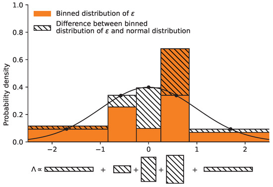
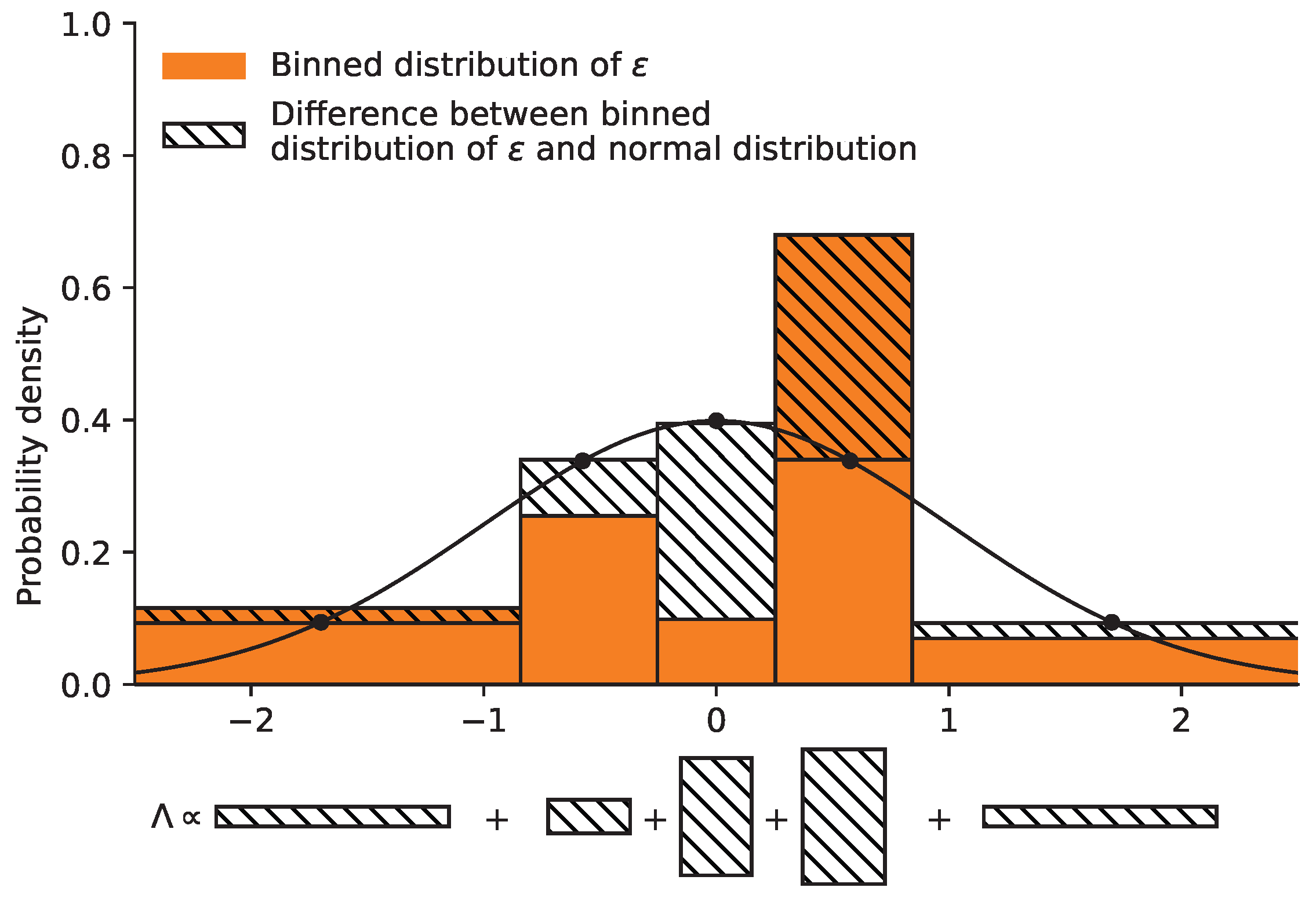
The quantity is accumulated over all dataset entries. The resulting histogram of is compared to that of standard normal distribution, as shown in Figure 1. For accurate uncertainty estimates, there should be equal weight in each bin of histogram and the normal distribution histogram. The similarity between the two histograms is captured by quality of uncertainty :
where is the number of entries in the mth bin of M. Bins are chosen so that the normal distribution has equal weight of in each. The quantity ranges from 0 for perfect uncertainty estimates to 1 for poor uncertainty estimates. The prefactor normalizes to : in the worst case of all N entries concentrated in a single bin, the unnormalized sum equals , and multiplication by rescales this to 1.
Figure 1.
Distribution of (orange) and standard normal distribution (white). Hatched regions represent the difference between the two distributions. The schematic at the bottom illustrates the addition of the differences to obtain .
We now calculate uncertainty in . Assuming N is large and the number of bins in the histogram is chosen to be [51]. This can be checked by performing the formal numerical optimization procedure in [38], which we repeat here to confirm that the optimal number of bins is for large N. With this choice of M, the quality of uncertainty becomes:
The number of points in the mth bin, , obeys normal distribution for large N, i.e., ∼, and therefore ∼ where denotes the folded normal distribution [52]. The uncertainty in is therefore:
Other metrics that quantify how good uncertainty estimates are include expected normalized calibration error ENCE [39] and normalized mean rescaled confidence interval n-MeRCI [53]. However, ENCE only considers variance of errors in predictions rather than histogram of these errors, meaning ENCE may not capture as much detail about uncertainty estimates as . The n-MeRCI metric requires knowledge about outliers in the underlying data, which limits the scope of its application compared to . Furthermore, these do not give a readily derived analytic expression. Therefore, we adopt quality of uncertainty for the remainder of this study.
The derivation above relies on several assumptions: approximately normal residual behavior, large-N approximations, and the binning choice . These assumptions are used to obtain a closed-form uncertainty estimate for and hence a transparent expression for the weighting coefficient. We therefore interpret the resulting metric as an analytically motivated objective under these assumptions, rather than a universal optimum for all data regimes.
Regarding the bin count, we use as a standard histogram scaling rule and for consistency with the asymptotic derivation of . Alternative values of M are possible and may change the numerical value of ; therefore, sensitivity to M should be examined in extended empirical studies.
2.3. Combined Metric
We have now defined the metrics and . However, each of these takes its best value at different hyperparameters, but we need to select a single set of hyperparameters that reaches the best compromise between and . To achieve this, we juxtapose and into a single combined metric. The simplest combined form is a superposition:
where is a positive coefficient (that we ultimately derive as a function of ), which ensures that higher values of and lower values of are favored. Overall a large value of this metric is better, and it takes a peak value of 1. In the following derivation, we focus on standard uncertainty propagation as this will (1) allow us to derive a closed-form expression for that is based on the uncertainties in and and (2) is accessible and builds on well-understood components. Alternative approaches to combining and are possible, such as non-linear combinations or multi-objective optimization, but we focus on the linear superposition for its simplicity and interpretability.
We need to determine the best weighting factor . To do this, we first consider the metric in the generalized form:
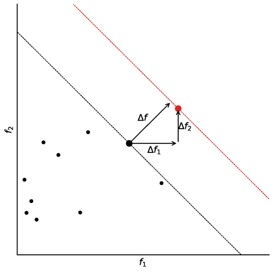
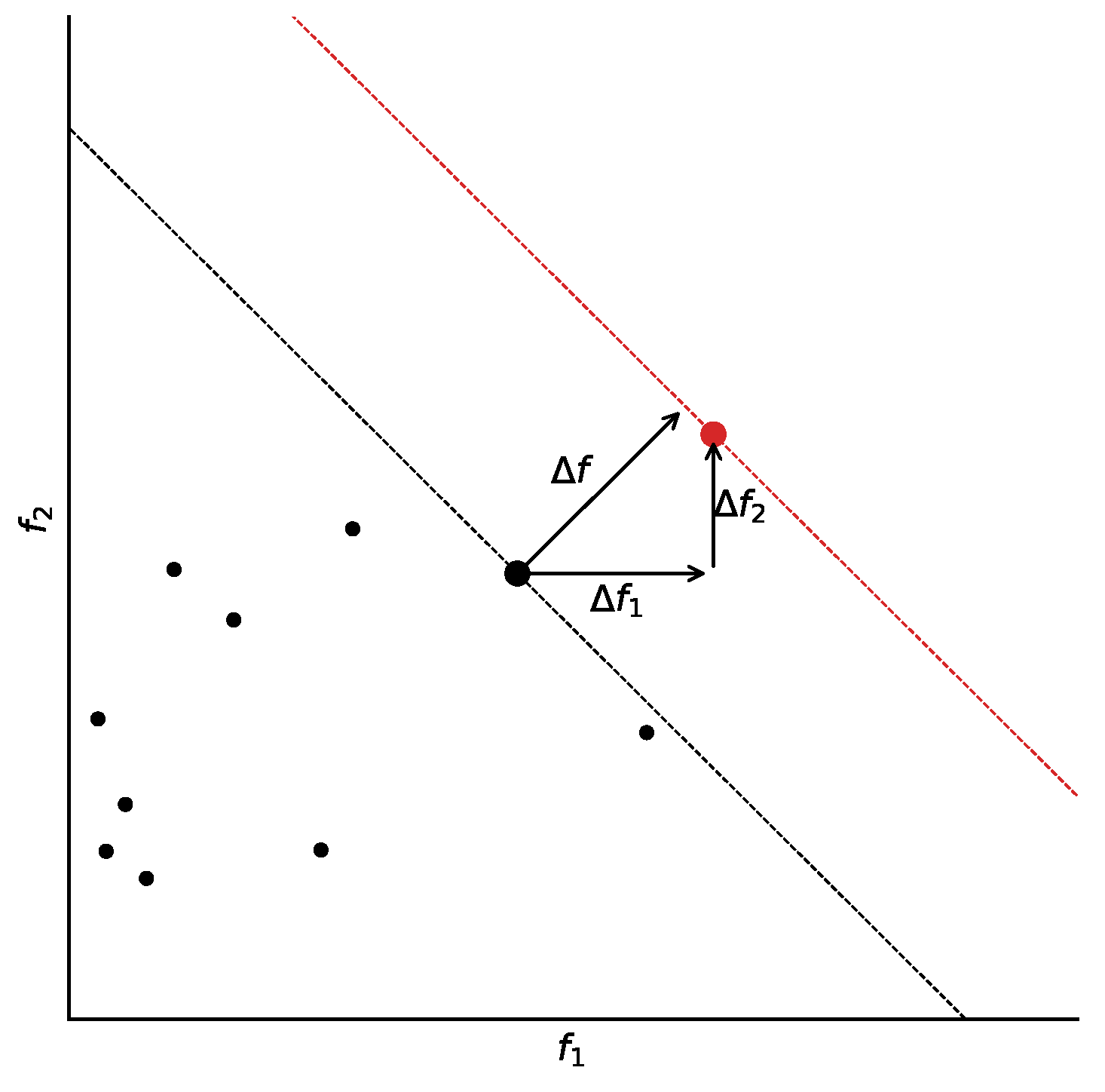
where , . We illustrate cross-validation values of against for different sets of hyperparameters in Figure 2. The maximum of the expected value of , which is the true maximum we seek, is represented by the black point that lies on the black line. However, the data available for cross-validation likely contains noise, which is propagated through to uncertainty in both and , so spurious maxima of will arise. One example is represented by the red point on the red line in Figure 2.
Figure 2.
Plot of against for different sets of hyperparameters. The black dashed line at 45 degrees carries a point that is the true maximum of . The red dashed line at 45 degrees carries a point that arises from noise, and is the spurious maximum of . Other black points represent suboptimal hyperparameter sets.
We assume that noise in and is normally distributed with zero mean and standard deviation and , respectively. If an uncertain point arises at a distance along the -axis and along the -axis, the value of the metric differs from its expected value by:
In Figure 2, we highlighted the important example of a spurious maximum. The probability density distribution of , denoting as , is:
From this equation, it follows that ∼. During hyperparameter optimization, we wish to find the robust maximum that avoids overfitting. This is achieved when the metric has small uncertainty so we can be confident in its value, i.e., we minimize the standard deviation of . Assuming the density of points at the true maximum is fixed, we vary the ratio , and find that standard deviation of is the smallest when , i.e., . In other words, the maximum of is most confidently identified when noise in has the same standard deviation as noise in . This leads to the following expression for :
and so the combined metric is the non-linear:
As , the combined metric approaches . This is desirable behaviour, as when predictions are perfect, the bootstrapping methodology will correctly give infinitesimal uncertainties, and so becomes irrelevant. As decreases, the combined metric places more emphasis on , which allows uncertainty to steer us clear of poor predictions.
Alternative weighting strategies are also possible, including fixed user-defined , normalization by empirical standard deviations, or explicit multi-objective (Pareto) search. We chose the condition because it gives a closed-form, uncertainty-balanced weighting with minimal additional tuning in the present setting.
Accordingly, we position the method as a practically useful scalarization, not as a fundamentally new learning paradigm. The contribution is methodological: it provides a transparent uncertainty-aware objective for model selection when practitioners require a single score that jointly reflects prediction fidelity and uncertainty quality.
3. Validation of Combined Metric
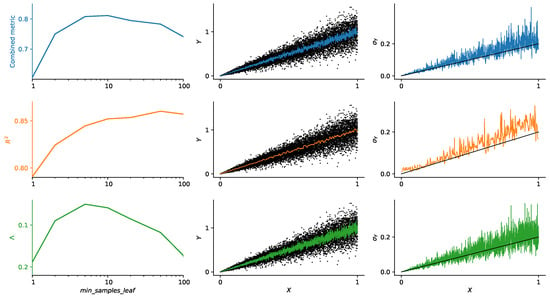
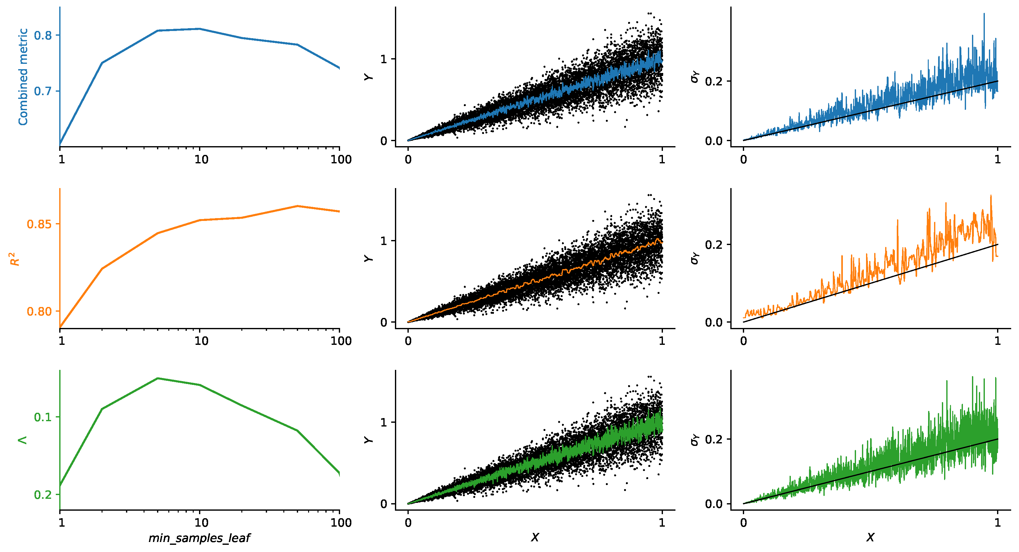
Having derived the combined metric, we now validate that its optimization leads to better overall estimates of expected value and uncertainty compared to optimization of either alone or alone. We focus on the paradigmatic problem of fitting a straight line, though the underlying data has increasing amplitude of noise going up the line (see Figure 3). First, in Section 3.1, we identify and train three machine learning models that lead to the best values of firstly our proposed combined metric, secondly , and thirdly , respectively. Then, in Section 3.2, we compare predictions of the output variable and its uncertainty from the three models. Finally, in Section 3.3, to mimic a real-life design problem, we apply the three models to calculate probability that the output variable satisfies a target, and compare the results.
Figure 3.
(Leftmost panel): plots of combined metric (blue), (orange), and (green) against . (Central panel): predictions of Y from the models that optimize combined metric (blue), (orange), and (green), alongside true values of Y (black points). (Rightmost panel): estimates of uncertainty in Y, , from the models that optimize combined metric (blue), (orange), and (green), alongside true values of (black line).
3.1. Machine Learning Models
We require a model that is computationally cheap and makes uncertainty estimates in its predictions, so we adopt random forest, implemented in Scikit-learn Python package version 1.8.0 [12]. Random forest is a collection of independent identical regression trees. During the training phase, each tree learns the map from input to output. Predictions of the trees are then averaged to give the overall prediction, and their standard deviation is used to calculate uncertainty estimate in this prediction. The hyperparameter of random forest model that we vary is , which is the minimum number of datapoints in each leaf of a regression tree. Because each leaf averages across at least datapoints, standard deviation of predictions of the trees is multiplied by to give an estimate of machine learning uncertainty, and is itself used as an estimate of experimental uncertainty. Testing confirms that this scaling gives the correct standard deviation of the underlying data in this controlled setup as local averaging within leaves is the dominant smoothing mechanism; we treat it as a modeling assumption rather than a universally valid uncertainty estimator. We adopt a paradigmatic dataset comprising N = 10,000 entries and two columns—X and Y. We define X as the input variable and Y as the output variable. X is uniformly distributed between 0 and 1, and Y∼. As a demonstrative example, we use that ensures a strong amplitude of noise without overwhelming the underlying function, and have confirmed that similar performance is achieved for other values of .
We now train several machine learning models, each with a different value of . We calculate the combined metric, , and , for each value using 5-fold cross-validation method [48]. We plot the values of combined metric, , and in Figure 3. The optimal value of combined metric is achieved when . The optimal value of is achieved when ; this is because random forest averages the noise across more datapoints, which leads to better predictions. The optimal value of is achieved when ; this is because a small number of samples in a leaf allows to accurately capture the local scatter in data and therefore leads to the best uncertainty estimates.
The model that optimizes combined metric gives and , achieving the best compromise between and . The model that optimizes has smaller fluctuations in estimates of expected value compared to the other two models due to larger , but systematically overestimates uncertainty. The model that optimizes has large fluctuations in expected value compared to the other two models due to smaller , but gives uncertainty estimates that are on average closest to the true values.
This behavior is consistent with a bias-variance style trade-off in the mean prediction coupled to uncertainty ranking quality. Large leaves reduce mean-estimate variance but can smooth out local heteroscedastic structure; very small leaves capture local scatter but increase prediction noise. The combined objective tends to select an intermediate regime where both effects are balanced.
3.2. Validation of Machine Learning Predictions
While accurate predictions across the entire dataset are desirable, in real-world applications it is important to focus on the most confident and robust predictions—the ones with the lowest uncertainty [54,55,56,57]. As an example, we consider the design of a drug that targets a novel disease. Several drug designs could be effective, but the design with the highest confidence in its effectiveness would be deployed to achieve the fastest and therefore the most efficient immunization of the population [58]. It is therefore desirable that predictions with low uncertainty are closer to the true value than predictions with high uncertainty. As we discard high uncertainty predictions, we expect the error in predictions across the remaining entries to decrease.
We now validate that the model that optimizes combined metric gives better predictions than the other two models as we focus on just the most confident predictions. We focus on three datasets: the linear dataset studied in the previous section, secondly a real-world benchmark dataset that models wine quality, and thirdly a a real-world benchmark dataset that models productivity of garment manufacturers.
3.2.1. Paradigmatic Linear Dataset
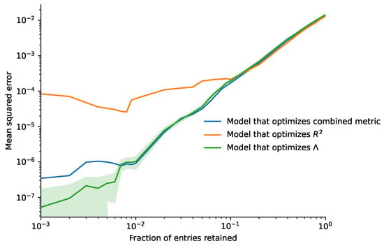
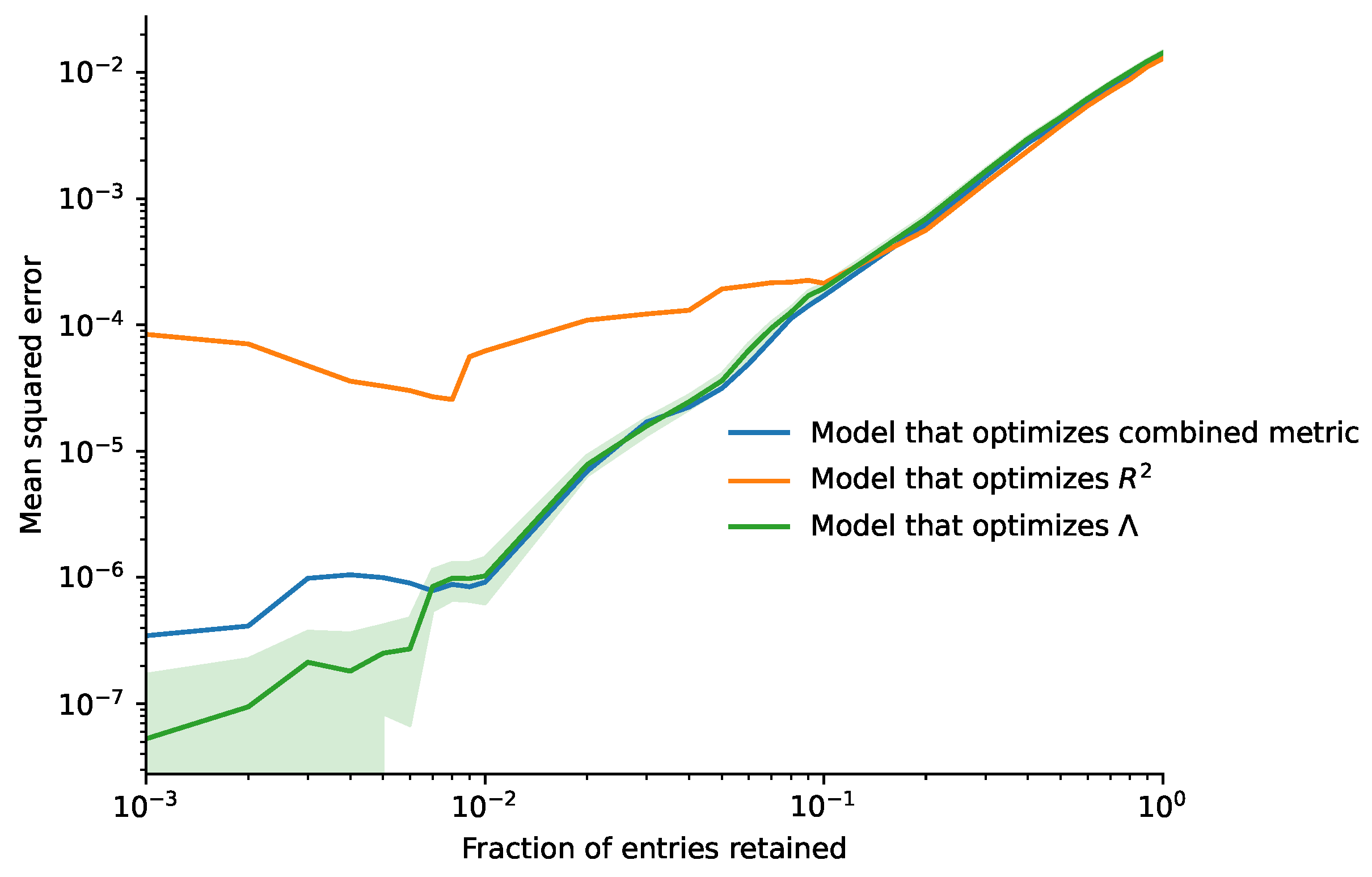
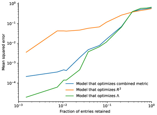
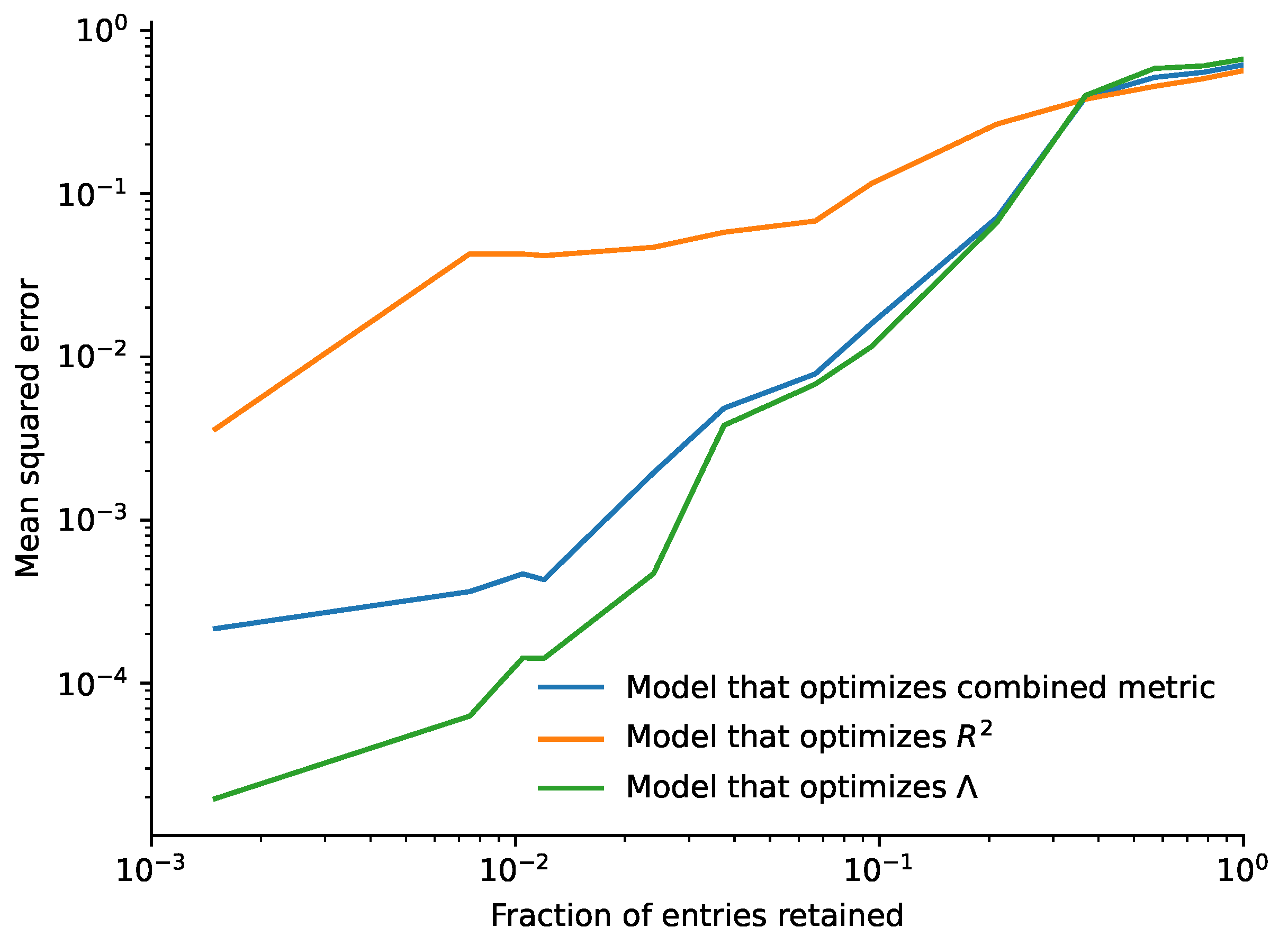
We take the three optimal models from the previous section, and analyze a fresh blind dataset with 10,000 rows from the same distribution Y∼ with . We then discard entries where predictions have high uncertainty, and compute mean squared error in predictions of Y for the entries retained. We perform this calculation for a range of fractions of entries retained, and in Figure 4 we plot mean squared error in Y against fraction of entries retained for the three models.
Figure 4.
Mean squared error (MSE) in predictions for the linear dataset from the model that optimizes combined metric (blue), model that optimizes (orange), and model that optimizes (green), plotted against the fraction of entries retained. The shaded green area represents the range of results obtained by repeating the analysis with 100 different random number seeds.
When all entries are retained, the model that optimizes gives the lowest mean squared error in predictions, which is expected. As fraction of entries retained decreases, mean squared error from all three models decreases. At fraction of entries retained <0.1, mean squared error from the models that optimize combined metric and eventually becomes smaller than mean squared error from the model that optimizes . The model that optimizes plateaus in the graph as the error in its predictions is obscured by the poor understanding of uncertainty. Interestingly, this occurs at the fraction of entries retained <0.1, similar to the fractional error in the uncertainty histogram in Figure 1, also 0.1.
As we continue to decrease the fraction of entries retained, focusing on just the most confident predictions, the model that optimizes combined metric is still better than the other two. The improvement of the combined metric over the optimized model in the region of fraction of entries retained <0.1 has a Wilcoxon signed-rank (two-sided) , which is strong statistical evidence for the improvement offered by the combined metric. Finally, when the fraction of entries retained becomes 0.008, the model that optimizes becomes better than the other two. However, this is a very small fraction of the data, and model error is <, so for practical purposes the model that optimizes combined metric is the most useful.
In real-life design problems, there are often several possible solutions that satisfy the target criteria, and the machine learning technique only needs to identify one of them. Therefore, retaining just a fraction of predictions is in line with this real-life workflow, and optimizing combined metric is therefore highly desirable for real-life applications, delivering a 400-times improvement in mean squared error.
Finally, we repeat the analysis but with a different random number seed, which we repeat 100 several times. This allows us to understand the distribution range of the results and understand its statistical significance. The range of results is shown by the shaded area in Figure 4. We observe a narrow distribution, confirming the statistical significance of the main trend that the model that optimizes combined metric gives the best overall compromise.
3.2.2. Wine Dataset
The dataset comprises both the red and white variants of the Portuguese “Vinho Verde” wine [59]. The dataset focuses on physicochemical input variables and sensory output variables, summarized as a perceived “quality” score. The classes are ordinal and imbalanced, with substantially more wines of average quality than of either exceptional or poor quality.
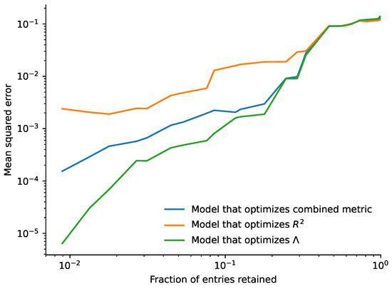
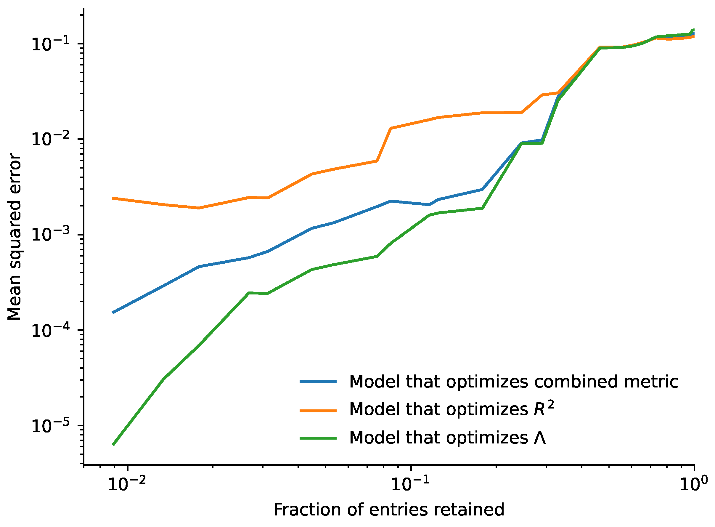
The fitting performance is shown in Figure 5. The root mean-square error in quality when predictions are made over all data is ∼0.6. This represents a good fit for a wine quality score rated 0–10, i.e., it is smaller than the interval between adjacent wine quality scores, and is also highly respectable compared to other methods on this benchmark dataset. However, this is when making predictions over all data, we now look in detail and performance when we focus on the most confident predictions.
Figure 5.
Mean squared error (MSE) in predictions for the wine dataset from the model that optimizes combined metric (blue), the model that optimizes (orange), and the model that optimizes (green), plotted against fraction of entries retained.
When all entries are retained, the -optimized model has the lowest mean squared error. As the retained fraction decreases below 0.3, the combined-metric and -optimized models outperform it, while the -optimized model uncertainty is poorly resolved so it does not further improve. Although the -optimized model is best at a retained fraction of below 0.05, this involves very little data and an error below 0.001, so the combined-metric model is the most practical.
3.2.3. Garment Dataset
The garment industry is a prominent example of industrial globalization in the modern era. As a highly labour-intensive sector characterized by numerous manual processes, its ability to meet global demand depends substantially on the productivity and delivery performance of employees. Accordingly, it is of considerable interest to industry decision makers to monitor, analyse, and predict the productivity. The dataset [60] focuses on team human resource input variables, with productivity as the output.
The fitting performance is shown in Figure 6. The root-mean-square error in productivity predictions across the full dataset is approximately 0.12; this compares well against a productivity score on a 0–1 scale, representing a typical error of just that compares favourably with other methods on this benchmark. We next consider how when attention is restricted to the most confident predictions performance can improve yet further.
Figure 6.
Mean squared error (MSE) in predictions for the garments dataset from the model that optimizes combined metric (blue), model that optimizes (orange), and model that optimizes (green), plotted against fraction of entries retained.
The -optimized model yields the lowest mean squared error when it is validated against all available data. However, if we make predictions for just the 0.4 most confident values, overall performance increases but in particular both the combined-metric and -optimized models become more accurate than the -optimized model, because the latter has worse estimates of its uncertainty. The -optimized model performs best when predicting the fraction 0.3 of most confident values.
In all three datasets, the model that optimizes combined metric gives better predictions than the other two models as we focus on just the most confident predictions. This is desirable for real-world applications, where we want to identify the most confident and robust predictions. Furthermore, our tests confirm the generality of the proposed metric, and that we therefore expect it to perform on real-world non-linear, noisy, and complex datasets.
3.3. Application to Design
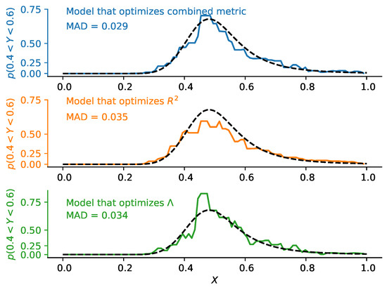
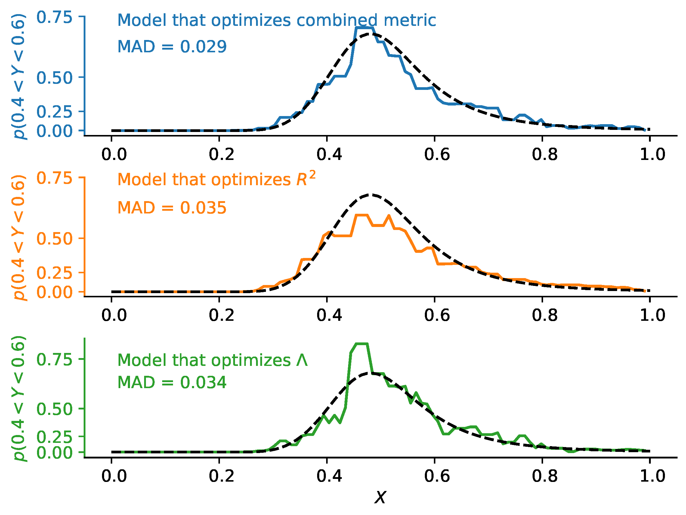
Having validated predictions of the three machine learning models that optimize combined metric, , and respectively, we now apply these models to calculate the probability that the output variable satisfies the target, as would be done in a real-world design problem. We set the target for Y to be . Using each of the three models, we calculate the probability of meeting the target for each value of input X. The probability of meeting the target from each model with 3-point median filtering [61] applied is plotted in Figure 7 alongside theoretical probability of meeting the target.
Figure 7.
Probability of Y meeting the target , calculated from the model that optimizes the combined metric (blue), the model that optimizes (orange), and the model that optimizes (green). Theoretical probability is represented by black dashed line in each plot. MAD is the mean absolute difference between the two curves in each corresponding plot.
The similarity between the probability predictions from each model and theoretical probabilities is quantified by mean absolute difference (MAD) between the two curves. The values of MAD for each model are displayed in Figure 7. The value of MAD is the smallest for the model that optimizes combined metric. Therefore, probability predictions from the model that optimizes combined metric are more similar to theoretical probabilities compared to the other two models.
The model that optimizes gives probabilities that are generally further away from theoretical probabilities compared to the other two models. The model that optimizes gives good probability predictions, but these predictions have more noise in them compared to predictions from the model that optimizes combined metric. Overall, the model with hyperparameter value that optimizes combined metric gives the best probability predictions out of the three, meaning that optimizing the combined metric is beneficial for design problems.
The absolute performance differences in this benchmark are modest (e.g., MAD differences on the order of to ), so results should be interpreted as evidence of a consistent trend in this controlled scenario rather than a definitive practical gain in all applications. A stronger statistical assessment with repeated runs, confidence intervals, and formal significance tests is an important next step.
4. Conclusions
We derive a combined metric for assessing the quality of fit of a machine learning model, which incorporates both coefficient of determination , and quality of uncertainty . The combined metric is of form , with coefficient . In both the controlled benchmark used here and also real-life datasets on wine and garments production, a model with hyperparameters that optimize the combined metric gives better-balanced predictions of output variable and its uncertainty compared to optimizing alone. We note that other metrics for model and uncertainty quality are possible, but the choice of and has not only shown that the combined metric is beneficial, but moreover delivered a simple analytic and interpretable metric.
For practical deployment, we envisage the following workflow: (i) train candidate models under cross-validation, (ii) compute , , and the combined metric on each fold, (iii) select hyperparameters by maximizing the combined metric, (iv) calibrate uncertainty if required by downstream risk tolerance, and (v) validate on a blind or shifted test set using both prediction and uncertainty diagnostics. This pathway makes the method operational in application-focused studies. Indeed, since early 2025 the approach has been used in a commercial setting by Intellegens Ltd. (Cambridge, UK), which has given its customers access to improved model selection for regression problems where uncertainty is important. The approach has therefore been used across a range of applications, including materials design, drug design, chemical engineering, and fast moving consumer goods.
The combined metric can be used to evaluate performance of machine learning regression models in applications that demand high quality of both output variable predictions and uncertainty estimates. Potential examples include materials design and drug design, where not only the value of the output variable, but also its uncertainty is crucial to identify the configuration that will most likely work. Furthermore, in applications where the value of uncertainty itself can be a useful input for predicting the final quantity of interest [62], the combined metric may help identify models that give better uncertainty estimates while retaining high prediction quality. Examples include additive manufacturing [63], information engineering [64], and financial markets [65]. These broader applications remain hypotheses to be validated in domain-specific studies.
While the combined metric in this work improves results for regression, similar ideas may be explored for classification and unsupervised learning. As an example, one could consider prediction of cancer at early stages, where identification of reliable low-uncertainty predictions is critical [66,67]. Likewise, uncertainty-aware variants of clustering criteria could be investigated for stable clustering under perturbations [68,69,70].
Author Contributions
Conceptualization: B.Z.; Formal analysis: B.Z.; Funding acquisition: G.C.; Investigation: B.Z.; Methodology: B.Z.; Project administration: G.C.; Software: B.Z.; Supervision: G.C.; Validation: B.Z.; Visualization: B.Z.; Writing—original draft: B.Z.; Writing—review and editing: G.C. All authors have read and agreed to the published version of the manuscript.
Funding
The authors acknowledge the financial support of the Engineering & Physical Sciences Research Council, the Royal Society, and Harding Distinguished Postgraduate Scholars Programme Leverage Scheme.
Institutional Review Board Statement
Not applicable.
Informed Consent Statement
Not applicable.
Data Availability Statement
The synthetic data-generation protocol and evaluation definitions are fully specified in the manuscript. Data used for machine learning is available at https://archive.ics.uci.edu (accessed on 21 July 2026).
Conflicts of Interest
Gareth Conduit is a Director of the machine learning company Intellegens. The authors have no other financial interests or personal relationships that could have appeared to influence the work reported in this paper.
References
- Andersen, C.W.; Armiento, R.; Blokhin, E.; Conduit, G.J.; Dwaraknath, S. OPTIMADE, an API for exchanging materials data. Nat. Sci. Data 2021, 8, 217. [Google Scholar] [CrossRef] [Scilit] [PubMed]
- NoMaD. 2017. Available online: https://nomad-lab.eu/index.php?page=repo-arch (accessed on 21 July 2026).
- MatWeb. 2017. Available online: http://www.matweb.com/ (accessed on 21 July 2026).
- Bishop, C.M. Pattern Recognition and Machine Learning; Springer: Berlin/Heidelberg, Germany, 2006. [Google Scholar]
- Guerney, K. An Introduction to Neural Networks; UCL Press: London, UK, 1997. [Google Scholar]
- Krizhevsky, A.; Sutskever, I.; Hinton, G.E. ImageNet Classification with Deep Convolutional Neural Networks. In Proceedings of the Advances in Neural Information Processing Systems; Curran Associates, Inc.: New York, NY, USA, 2012; Volume 25. [Google Scholar]
- He, K.; Zhang, X.; Ren, S.; Sun, J. Deep Residual Learning for Image Recognition. In Proceedings of the 2016 IEEE Conference on Computer Vision and Pattern Recognition (CVPR), Las Vegas, NV, USA, 27–30 June 2016; pp. 770–778. [Google Scholar] [CrossRef] [Scilit]
- Karpathy, A.; Toderici, G.; Shetty, S.; Leung, T.; Sukthankar, R.; Fei-Fei, L. Large-Scale Video Classification with Convolutional Neural Networks. In Proceedings of the 2014 IEEE Conference on Computer Vision and Pattern Recognition, Columbus, OH, USA, 23–28 June 2014; pp. 1725–1732. [Google Scholar] [CrossRef] [Scilit]
- Heskes, T. Selecting Weighting Factors in Logarithmic Opinion Pools. In Proceedings of the Advances in Neural Information Processing Systems; MIT Press: Cambridge, MA, USA, 1997; Volume 10. [Google Scholar]
- Tancret, F. Computational thermodynamics, Gaussian processes and genetic algorithms: Combined tools to design new alloys. Model. Simul. Mater. Sci. Eng. 2013, 21, 045013. [Google Scholar] [CrossRef] [Scilit]
- Petit, S.J.; Bect, J.; Feliot, P.; Vazquez, E. Parameter Selection in Gaussian Process Interpolation: An Empirical Study of Selection Criteria. SIAM/ASA J. Uncertain. Quantif. 2023, 11, 1308–1328. [Google Scholar] [CrossRef] [Scilit]
- Pedregosa, F.; Varoquaux, G.; Gramfort, A.; Michel, V.; Thirion, B.; Grisel, O.; Blondel, M. Scikit-learn: Machine Learning in Python. J. Mach. Learn. Res. 2011, 12, 2825–2830. [Google Scholar]
- Bhadeshia, H.K.D.H.; MacKay, D.J.C.; Svensson, L.E. Impact toughness of C-Mn steel arc welds—Bayesian neural network analysis. Mater. Sci. Technol. 1995, 11, 1046–1051. [Google Scholar] [CrossRef] [Scilit]
- Sourmail, T.; Bhadeshia, H.; MacKay, D.J.C. Neural network model of creep strength of austenitic stainless steels. Mater. Sci. Technol. 2002, 18, 655–663. [Google Scholar] [CrossRef] [Scilit]
- Agrawal, A.; Deshpande, P.D.; Cecen, A.; Basavarsu, G.P.; Choudhary, A.N.; Kalidindi, S.R. Exploration of data science techniques to predict fatigue strength of steel from composition and processing parameters. Integr. Mater. Manuf. Innov. 2014, 3, 90–108. [Google Scholar] [CrossRef] [Scilit]
- Ward, L.; Agrawal, A.; Choudhary, A.; Wolverton, C. A general-purpose machine learning framework for predicting properties of inorganic materials. npj Comput. Mater. 2016, 2, 16028. [Google Scholar] [CrossRef] [Scilit]
- Legrain, F.; Carrete, J.; van Roekeghem, A.; Curtarolo, S.; Mingo, N. How Chemical Composition Alone Can Predict Vibrational Free Energies and Entropies of Solids. Chem. Mater. 2017, 29, 6220–6227. [Google Scholar] [CrossRef] [Scilit]
- Gomberg, J.A.; Medford, A.J.; Kalidindi, S.R. Extracting knowledge from molecular mechanics simulations of grain boundaries using machine learning. Acta Mater. 2017, 133, 100–108. [Google Scholar] [CrossRef] [Scilit]
- Ubaru, S.; Mikeldar, A.; Saad, Y.; Chelikowsky, J.R. Formation enthalpies for transition metal alloys using machine learning. Phys. Rev. B 2017, 95, 214102. [Google Scholar] [CrossRef] [Scilit]
- Lee, J.; Seko, A.; Shitara, K.; Nakayama, K.; Tanaka, I. Prediction model of band gap for inorganic compounds by combination of density functional theory calculations and machine learning techniques. Phys. Rev. B 2016, 93, 115104. [Google Scholar] [CrossRef] [Scilit]
- Ward, L.; Liu, R.; Krishna, A.; Hegde, V.I.; Agrawal, A.; Choudhary, A.; Wolverton, C. Including crystal structure attributes in machine learning models of formation energies via Voronoi tessellations. Phys. Rev. B 2017, 96, 024104. [Google Scholar] [CrossRef] [Scilit]
- Khurana, D.; Koli, A.; Khatter, K.; Singh, S. Natural language processing: State of the art, current trends and challenges. Multimed. Tools Appl. 2023, 82, 3713–3744. [Google Scholar] [CrossRef] [Scilit] [PubMed]
- Gillioz, A.; Casas, J.; Mugellini, E.; Abou Khaled, O. Overview of the Transformer-based Models for NLP Tasks. In Proceedings of the 2020 Federated Conference on Computer Science and Information Systems, Sofia, Bulgaria, 6–9 September 2020; pp. 179–183. [Google Scholar] [CrossRef] [Scilit]
- Zerva, C.; Batista-Navarro, R.; Day, P.; Ananiadou, S. Using uncertainty to link and rank evidence from biomedical literature for model curation. Bioinformatics 2017, 33, 3784–3792. [Google Scholar] [CrossRef] [Scilit] [PubMed]
- Goujon, B. Uncertainty Detection for Information Extraction. In Proceedings of the International Conference RANLP-2009, Borovets, Bulgaria, 14–16 September 2009. [Google Scholar]
- Lee, A.; Lin, M.C.; Kao, R.T.; Chen, K.T. An Effective Clustering Approach to Stock Market Prediction. In Proceedings of the PACIS 2010 Proceedings, Taipei, Taiwan, 9–12 July 2010; Volume 54. [Google Scholar]
- Martin, D.; Póczos, B. Machine learnin g-aided modeling of fixed income instruments. In Proceedings of the Thirty-Second Conference on Neural Information Processing Systems, Montréal, QC, Canada, 3–8 December 2018. [Google Scholar]
- Zhang, L. A General Framework of Derivatives Pricing. J. Math. Financ. 2020, 10, 255–266. [Google Scholar] [CrossRef]
- Chicco, D.; Warrens, M.; Jurman, G. The coefficient of determination R-squared is more informative than SMAPE, MAE, MAPE, MSE and RMSE in regression analysis evaluation. Peerj Comput. Sci. 2021, 7, e623. [Google Scholar] [CrossRef] [Scilit] [PubMed]
- Forsdyke, J.; Zviazhynski, B.; Lees, J.; Conduit, G. Probabilistic selection and design of concrete using machine learning. Data Centric Eng. 2023, 4, e9. [Google Scholar] [CrossRef] [Scilit]
- Conduit, B.D.; Jones, N.G.; Stone, H.J.; Conduit, G.J. Design of a nickel-base superalloy using a neural network. Mater. Des. 2017, 131, 358. [Google Scholar] [CrossRef] [Scilit]
- Conduit, B.D.; Jones, N.G.; Stone, H.J.; Conduit, G.J. Probabilistic design of a molybdenum-base alloy using a neural network. Scr. Mater. 2018, 146, 82. [Google Scholar] [CrossRef] [Scilit]
- Conduit, B.D.; Illston, T.; Baker, S.; Duggappa, D.V.; Harding, S.; Stone, H.J.; Conduit, G.J. Probabilistic neural network identification of an alloy for direct laser deposition. Mater. Des. 2019, 168, 107644. [Google Scholar] [CrossRef] [Scilit]
- Dehghannasiri, R.; Xue, D.; Balachandran, P.V.; Yousefi, M.R.; Dalton, L.A.; Lookman, T.; Dougherty, E.R. Optimal experimental design for materials discovery. Comput. Mater. Sci. 2017, 129, 311. [Google Scholar] [CrossRef] [Scilit]
- Xue, D.; Balachandran, P.V.; Hogden, J.; Theiler, J.; Xue, D.; Lookman, T. Accelerated search for materials with targeted properties by adaptive design. Nat. Commun. 2016, 7, 11241. [Google Scholar] [CrossRef] [Scilit] [PubMed]
- Smith, J.S.; Nebgen, B.; Lubbers, N.; Isayev, O.; Roitberg, A.E. Less is more: Sampling chemical space with active learning. J. Chem. Phys. 2018, 148, 241733. [Google Scholar] [CrossRef] [Scilit] [PubMed]
- Verpoort, P.C.; MacDonald, P.; Conduit, G.J. Materials data validation and imputation with an artificial neural network. Comput. Mater. Sci. 2018, 147, 176. [Google Scholar] [CrossRef] [Scilit]
- Taylor, P.L.; Conduit, G. Machine learning predictions of superalloy microstructure. Comput. Mater. Sci. 2021, 201, 110916. [Google Scholar] [CrossRef] [Scilit]
- Levi, D.; Gispan, L.; Giladi, N.; Fetaya, E. Evaluating and Calibrating Uncertainty Prediction in Regression Tasks. Sensors 2022, 22, 5540. [Google Scholar] [CrossRef] [Scilit] [PubMed]
- Kuleshov, V.; Fenner, N.; Ermon, S. Accurate Uncertainties for Deep Learning Using Calibrated Regression. In Proceedings of the 35th International Conference on Machine Learning, PMLR, Stockholm, Sweden, 10–15 July 2018; Dy, J., Krause, A., Eds.; Proceedings of Machine Learning Research: Valencia, Spain, 2018; Volume 80, pp. 2796–2804. [Google Scholar]
- Song, H.; Diethe, T.; Kull, M.; Flach, P. Distribution calibration for regression. In Proceedings of the 36th International Conference on Machine Learning, PMLR, Long Beach, CA, USA, 9–15 June 2019; Chaudhuri, K., Salakhutdinov, R., Eds.; Proceedings of Machine Learning Research: Valencia, Spain, 2019; Volume 97, pp. 5897–5906. [Google Scholar]
- Deb, K.; Pratap, A.; Agarwal, S.; Meyarivan, T. A fast and elitist multiobjective genetic algorithm: NSGA-II. IEEE Trans. Evol. Comput. 2002, 6, 182–197. [Google Scholar] [CrossRef] [Scilit]
- Knowles, J. ParEGO: A hybrid algorithm with on-line landscape approximation for expensive multiobjective optimization problems. IEEE Trans. Evol. Comput. 2006, 10, 50–66. [Google Scholar] [CrossRef] [Scilit]
- Sener, O.; Koltun, V. Multi-Task Learning as Multi-Objective Optimization. In Proceedings of the Advances in Neural Information Processing Systems, Montréal, QC, Canada, 3–8 December 2018; Volume 31. [Google Scholar]
- Kendall, A.; Gal, Y.; Cipolla, R. Multi-Task Learning Using Uncertainty to Weigh Losses for Scene Geometry and Semantics. In Proceedings of the 2018 IEEE/CVF Conference on Computer Vision and Pattern Recognition, Salt Lake City, UT, USA, 18–23 June 2018; pp. 7482–7491. [Google Scholar] [CrossRef] [Scilit]
- Guo, C.; Pleiss, G.; Sun, Y.; Weinberger, K.Q. On Calibration of Modern Neural Networks. In Proceedings of the 34th International Conference on Machine Learning, Sydney, Australia, 6–11 August 2017; Volume 70, pp. 1321–1330. [Google Scholar]
- Gneiting, T.; Raftery, A.E. Strictly Proper Scoring Rules, Prediction, and Estimation. J. Am. Stat. Assoc. 2007, 102, 359–378. [Google Scholar] [CrossRef] [Scilit]
- Roberts, D.R.; Bahn, V.; Ciuti, S.; Boyce, M.S.; Elith, J.; Guillera-Arroita, G.; Hauenstein, S. Cross-validation strategies for data with temporal, spatial, hierarchical, or phylogenetic structure. Ecography 2017, 40, 913–929. [Google Scholar] [CrossRef] [Scilit]
- Pronzato, L.; Rendas, M.J.a. Weighted Leave-One-Out Cross Validation. SIAM/ASA J. Uncertain. Quantif. 2024, 12, 1213–1239. [Google Scholar] [CrossRef] [Scilit]
- Johnson, N.L.; Kotz, S.; Balakrishnan, N. Chi-Square Distributions including Chi and Rayleigh. In Proceedings of the Continuous Univariate Distributions, 2nd ed.; John Wiley and Sons: Cambridge, MA, USA, 1994; Volume 1, pp. 415–493. [Google Scholar]
- Lohaka, H. Making a Grouped-Data Frequency Table: Development and Examination of the Iteration Algorithm. Ph.D. Thesis, Ohio University, Athens, OH, USA, 2007. [Google Scholar]
- Liu, X.; Jin, Y.; Yang, Y.; Pan, X. Properties and Estimations of a Multivariate Folded Normal Distribution. Mathematics 2023, 11, 4860. [Google Scholar] [CrossRef] [Scilit]
- Moukari, M.; Simon, L.; Picard, S.; Jurie, F. n-MeRCI: A new Metric to Evaluate the Correlation Between Predictive Uncertainty and True Error. In Proceedings of the 2019 IEEE/RSJ International Conference on Intelligent Robots and Systems (IROS), Macau, China, 3–8 November 2019; Volume 11, pp. 5250–5255. [Google Scholar] [CrossRef] [Scilit]
- Irwin, B.; Mahmoud, S.; Whitehead, T.; Conduit, G.; Segall, M. Imputation versus prediction: Applications in machine learning for drug discovery. Future Drug Discov. 2020, 2, FDD38. [Google Scholar] [CrossRef] [Scilit]
- Mahmoud, S.Y.; Irwin, B.W.J.; Chekmarev, D.; Vyas, S.; Kattas, J.; Whitehead, T.M.; Mansley, T.; Bikker, J.; Conduit, G.J.; Segall, M.D. Imputation of Sensory Properties Using Deep Learning. J. Comput.-Aided Mol. Des. 2021, 35, 1125. [Google Scholar] [CrossRef] [Scilit] [PubMed]
- Irwin, B.W.J.; Levell, J.; Whitehead, T.M.; Segall, M.D.; Conduit, G.J. Practical Applications of Deep Learning to Impute Heterogeneous Drug Discovery Data. J. Chem. Inf. Model. 2020, 60, 2848. [Google Scholar] [CrossRef] [Scilit] [PubMed]
- Whitehead, T.M.; Irwin, B.W.J.; Hunt, P.A.; Segall, M.D.; Conduit, G.J. Imputation of Assay Bioactivity Data using Deep Learning. J. Chem. Inf. Model. 2019, 59, 1197. [Google Scholar] [CrossRef] [Scilit] [PubMed]
- Floresta, G.; Zagni, C.; Gentile, D.; Patamia, V.; Rescifina, A. Artificial Intelligence Technologies for COVID-19 De Novo Drug Design. Int. J. Mol. Sci. 2022, 23, 3261. [Google Scholar] [CrossRef] [Scilit] [PubMed]
- Cortez, P.; Cerdeira, A.; Almeida, F.; Matos, T.; Reis, J. Modeling wine preferences by data mining from physicochemical properties. Decis. Support Syst. 2009, 47, 547–553. [Google Scholar] [CrossRef] [Scilit]
- Imran, A.; Rahim, M.; Ahmed, T. Mining the productivity data of the garment industry. Int. J. Bus. Intell. Data Min. 2021, 19, 319. [Google Scholar] [CrossRef] [Scilit]
- Villar, S.; Torcida, S.; Acosta, G. Median Filtering: A New Insight. J. Math. Imaging Vis. 2017, 58, 130–146. [Google Scholar] [CrossRef] [Scilit]
- Zviazhynski, B.; Conduit, G. Unveil the unseen: Exploit information hidden in noise. Appl. Intell. 2023, 53, 11966–11978. [Google Scholar] [CrossRef] [Scilit]
- Rasiya, G.; Shukla, A.; Saran, K. Additive Manufacturing—A Review. Mater. Today Proc. 2021, 47, 6896–6901. [Google Scholar] [CrossRef] [Scilit]
- Płaczek, B.; Bernaś, M. Uncertainty-based information extraction in wireless sensor networks for control applications. Hoc Netw. 2014, 14, 106–117. [Google Scholar] [CrossRef] [Scilit]
- Sharpe, W. Mutual fund performance. J. Bus. 1966, 39, 119–138. [Google Scholar] [CrossRef] [Scilit]
- Hunter, B.; Hindocha, S.; RW, L. The Role of Artificial Intelligence in Early Cancer Diagnosis. Cancers 2022, 14, 1524. [Google Scholar] [CrossRef] [Scilit] [PubMed]
- Tobore, T. On the need for the development of a cancer early detection, diagnostic, prognosis, and treatment response system. Future Sci. OA 2019, 6, FSO439. [Google Scholar] [CrossRef] [Scilit] [PubMed]
- Shi, C.; Wei, B.; Wei, S.; Wang, W.; Liu, H.; Liu, J. A quantitative discriminant method of elbow point for the optimal number of clusters in clustering algorithm. EURASIP J. Wirel. Commun. Netw. 2021, 2021, 31. [Google Scholar] [CrossRef] [Scilit]
- Christakis, N.; Drikakis, D. Reducing Uncertainty and Increasing Confidence in Unsupervised Learning. Mathematics 2023, 11, 3063. [Google Scholar] [CrossRef] [Scilit]
- Liu, T.; Yu, H.; Blair, R.H. Stability estimation for unsupervised clustering: A review. Wires Comput. Stat. 2022, 14, e1575. [Google Scholar] [CrossRef] [Scilit] [PubMed]

Disclaimer/Publisher’s Note: The statements, opinions and data contained in all publications are solely those of the individual author(s) and contributor(s) and not of MDPI and/or the editor(s). MDPI and/or the editor(s) disclaim responsibility for any injury to people or property resulting from any ideas, methods, instructions or products referred to in the content. |
© 2026 by the authors. Licensee MDPI, Basel, Switzerland. This article is an open access article distributed under the terms and conditions of the Creative Commons Attribution (CC BY) license.