


Abstract
The acoustic frequency fingerprint (AFF) for drone recognition has emerged as a flexible and practical approach to address low-altitude airspace security concerns. However, three problems restrict its real-world application: (1) efficient AFF features are distributed across a wide range of frequencies, making them hard to extract accurately; (2) environmental noise originating from diverse sources, across different bands, cannot be denoised by a general method and limits monitoring accuracy; and (3) multi-band noise greatly increases the labeling workload and computational resources, limiting the flexibility in practical monitoring. This paper proposes a lightweight but efficient acoustic recognition system. We adopt a DE-filter and HLDWT to adaptively extract multi-band AFF features and limit other bands’ noises; a D-MPGAN to decouple and denoise motor and propeller characteristics, avoiding noisy sample labeling; and a lightweight MP-ResNet for motor and propeller feature handling, masking and comprehensive recognition decisions. Furthermore, we build a real dataset. Trained on clean 10 dB data and validated on −30 dB to 10 dB data, our system achieves 85% recognition accuracy at −30 dB with an inference time of 0.058 s/2000, outperforming mainstream methods trained on mixed noisy signals in anti-noise capability and efficiency, thus enabling reliable practical monitoring for low-altitude security.
1. Introduction
According to data analysis by Berg Insight [1], the commercial drone market already comprised 2.6 million unmanned aerial vehicle (UAV) units worldwide in 2024. This number is still increasing and is predicted to grow to around 6.9 million by around 2029. Due to the advantages of high flexibility, rapid flight speed, wide area coverage, and a wide variety of payloads, UAVs can easily perform complex tasks efficiently. Thus, UAVs are now widely utilized in aerial photography, transportation, disaster response, surveying and mapping, and various other fields. However, with the explosive growth of drones, security problems in low-altitude airspace are becoming more and more significant [2], such as illegal flights and attacks on airports, illegal surveillance of troops, etc. Therefore, an efficient and high-accuracy recognition technique is urgently needed for UAVs [3].
The explosion of drones has promoted research in UAV recognition technologies to enhance overall low-altitude security, including radar recognition, visible-spectrum imaging, infrared imaging, radio frequency (RF) sensing, acoustic recognition, etc.
Radar recognition: Radar target recognition relies on the radar cross-section (RCS), and this recognition is unaffected by severe weather and low-visibility scenarios [4]. However, compared with conventional aircraft, it is more difficult to calculate the RCS of UAVs due to their smaller size and special materials [5].
Visible-spectrum imaging and infrared imaging: YOLO nets are popular for object recognition in both visible-spectrum and infrared imaging [6,7,8]. In actual scenarios, YOLO nets, with a huge amount of parameters, are difficult to deploy on edge recognition devices. Moreover, the high complexity of image preprocessing and the substantial size of YOLO models can readily reduce the real-time recognition performance [8]. Furthermore, single-modal imaging is limited to adapting to different lighting conditions.
RF sensing: Electromagnetic signals are essential for UAVs to communicate with ground stations. Thus, RF-based recognition can fill a critical gap left by radar and imaging methods. It can directly identify UAVs through RF fingerprinting (RFF) technology [9,10], ignoring lighting conditions, target size, and material composition. However, many illegal UAVs may adopt a silent mode and not emit any signal to avoid recognition while approaching the target [11].
The above disadvantages of UAV recognition technologies have propelled the development of acoustic recognition [12,13,14], as all UAVs inevitably produce acoustic noise that is easily captured when UAVs approach their targets. Moreover, in environments with complex topographical obstacles, acoustic signals are often more detectable than RF signals or radar signals [15]. Furthermore, effective acoustic signals, which can be used for recognition, can be collected by much cheaper and simpler machines than the above signals collectors, thus can be more easily deployed on light machines or systems, enabling faster monitoring responses.
Since the acoustic noise of flying UAVs is mainly produced by the rotation of their propellers and motors, these components invariably carry various deviations introduced during manufacturing. These deviations form a unique and special acoustic frequency fingerprint (AFF) for each UAV, which has motivated research into the inherent characteristics of the propellers and motors during rotation. Generally, research on acoustic recognition focuses on two main directions: (i) how to achieve efficient AFF feature extractions based on acoustic signal processing techniques [16,17,18,19,20,21,22,23,24], and (ii) how to achieve accurate UAV identifications based on AFF feature distributions [25,26,27].
In the research on AFF feature extractions, early methods [16,17,18] proposed extracting spectrograms, which carry time–frequency features, as the primary acoustic signature for recognition. Mel-frequency cepstral coefficients (MFCC)-based UAV acoustic recognition has been explored in prior research [19,20], but these experiments were mainly conducted in high signal-to-noise ratio (SNR) conditions. Moreover, some researchers extracted, enhanced, and fused MFCC, gammatone frequency cepstral coefficients (GTCC), and various other acoustic features to enhance recognition performance in harsh environments [21,22]. Furthermore, some studies have proposed data augmentation to improve the robustness and accuracy of subsequent classifiers [23].
Based on AFF features, how to realize a high accurate identification also has a pivotal role in UAV acoustic recognition, and it is also an essential yet final step in UAV classification. In the past, recognition systems relied heavily on feature extraction, while employing only simple individual identification techniques, such as support vector machines (SVMs) [24], simple neural networks (NNs), Gaussian naive Bayes (GNB) classifiers, and k-nearest neighbor (KNN) algorithms [25]. With the significant advancement of deep learning (DL) methods in recent years, convolutional neural networks (CNNs), recurrent neural networks (RNNs), and enhanced CNNs [26,27] have been applied as classifiers for UAV recognition based on AFF features. These methods have also achieved significant progress and promoted the development of UAV acoustic recognition, decreasing the dependence on feature extractors to some extent.
Although UAV acoustic recognition techniques have achieved a lot in recent years and have been promoted to real environments, there are still many challenges at the practical level. Due to dynamic changes in the real environment, including wind variations, transmission channels fading and unknown acoustic noise from other devices, the received acoustic signals in the real environment always carry dynamic noises, which across multiple frequency bands and heavily destroy signals [28]. In addition, random sound sources in real-world environments and rotational changes of UAV propellers and motors for position shifting result in the AFF features also being distributed across multiple bands, which makes it difficult to extract efficient AFF features and heavily limits the robustness of the acoustic recognition system. Moreover, dynamic and random acoustic signals scatter at different frequency points, leading to difficulties in collecting, preprocessing and labeling useful signals, requiring more resources and destroying the convenience of practical acoustic recognition systems.
Thus, there are some urgent requirements that need to be addressed to resolve the above practical problems.
- (1)
- An entire system with both an effective feature extractor and a classifier is needed to correspond and be adaptive to AFF features distributed across dynamic, shifting frequency bands, and noises carrying different energy strengths in different bands. However, there is no complete system which can simultaneously reduce the impact of various acoustic noises and different UAV types on the frequency bands of AFF features and adapt to practical low-altitude airspace environments.
- (2)
- An efficient but robust AFF features extractor with a fast frequency bands filtering algorithm is required in dynamic and varied acoustic noise conditions. Some studies [21,22,23,25,26,27,28,29] were conducted to mitigate the impact of noise, but performed poorly especially at SNRs below −10 dB and lacked practical adaptability to varying noises in different frequency bands. To increase comprehensive performance, some studies [21,22] suggested that integrating different levels of MFCCs and more acoustic feature extraction algorithms could improve the robustness in harsh environments. But it is worth nothing that the recognition system depends on a feature extractor with extremely high computational complexity, which exhausts calculation resources, reduces real-time processing capability and still ignores the impact of frequency band distribution. A method of constructing robust datasets with sufficient variations was introduced in [28,29]. This approach can address problems in dynamic environments to a certain extent, but it resulted in excessive workloads for datasets preparation, labeling and training, achieving only limited improvements without limiting other bands’ noises.
- (3)
- A lightweight yet effective classifier is necessary for deployment in practical environments and real-time recognition. Even in the broader acoustic research, only one study has proposed adding a DL-based noise reduction step to enhance the system robustness, which may be able to alleviate the burden of classifiers [30]. Other studies, like [16,17,18], proposed that transforming acoustic signals into spectrograms can achieve better AFF feature distributions for DL classifiers, simplifying the classification task. However, spectrograms often require deeper networks to extract features, which also undermines their suitability for deployment on edge devices. Besides, many works have enhanced the accuracy and robustness in the presence of dynamic noise by improving DL classification networks based on recent popular approaches, including multiple CNN modules [21,31], ResNet with multiple layers [12], YOLO nets [32], transformers [33] and even attention mechanisms [28,34]. Although improved DL classification networks have significantly advanced traditional UAV acoustic classification, most of these complex networks require extensive parameter tuning and are difficult to deploy on edge devices for practical use. Moreover, if without abundant training data covering various SNRs, they also perform poorly in real environments with dynamic noise.
This article introduces an entire acoustic recognition system to resolve these urgent problems of AFF performance unreliability in a wide frequency band, dynamic interferences from various sound sources, and the difficulty of deploying large networks on edge devices, using five distinct and targeted methods that include high dynamic signal processing algorithms, and lightweight DL networks highly targeted to efficiently handle decoupled features. The main contributions of this article are summarized as follows and the overview of our system is depicted in Figure 1:
Figure 1.
Overview of our system: DE-filter and HLDWT jointly decouple multiple frequency bands and extract distinctive denoised AFF features; D-MPGAN further transfers denoised AFF features to clean AFF features and decouples them into motor features (MF) and propeller features (PF); MP-ResNet separately processes and fuses MP and MF comprehensively to acquire reliable and robust recognition results.
- (1)
- We propose a dynamic energy filter (DE-filter) to extract the main required acoustic signals carrying distinct fingerprint features while removing unwanted noises, enabling it to adapt quickly to changing environments and improve the robustness of the entire system. Acoustic signals received in real-world environments always carry various noises from different sound sources present in each frequency band. The key AFFs originate from the rotations of propellers and motors, so are mainly concentrated in a few special frequency bands. However, the key bands always have different frequency points, according to UAV movement and type. Thus, the DE-filter is a new algorithm based on energy and harmonic wave distributions to detect key feature frequency bands and dynamically extract the required acoustic signals from the special bands while eliminating unwanted noises across other frequencies, according to real-time analysis.
- (2)
- We present a dedicated and targeted UAV AFF feature extractor, HLDWT, based on the signal segment filtering by the DE-filter, to achieve more accurate features and reduce computational complexity in harsh real-world environments. The DE-filter decouples different frequency bands and removes noise in unimportant frequency bands, but other noise at key frequencies still remains. Thus, the HLDWT is proposed to separately extract high-frequency AFF (HAFF) features and low-frequency AFF (LAFF) features based on discrete wavelet transformation (DWT), with a simple structure. Furthermore, the HLDWT achieves a greater robustness by arranging and accumulating DWT decomposition layers with high-frequency features and low-frequency features in accordance with inherent band characteristics, which is advantageous for the best utilization of different frequency bands and leads to a highly accurate extraction.
- (3)
- We present a novel D-MPGAN incorporating two dedicated generators: a D-generator for decoupling noises from different frequency bands, and an MP-generator for decoupling motor and propeller features from mixed denoised features—based on features extracted from the DE-filter and HLDWT and completely addressing the problem of features and noises across multiple frequency bands. Moreover, the features generated by the D-MPGAN based on varying interfered data can be recognized by a classifier trained only on features from uninterfered data, which addresses the heavy labor work of collecting, processing, and labeling interfered data.
- (4)
- We propose a residual network based on the denoised features of motors and propellers (MP-ResNet), which constructs residual modules, a mask module and a feature fusion module based on denoised and decoupled features for the final classification task. Since the previous denoising process makes the features simple and precise, MP-ResNet can be composed of light residual modules for handling motor and propeller features, a mask module for assigning weight to decoupled features and a simple fusion module for final decision, which features a lightweight structure, highly robust recognition and a fast inference speed.
- (5)
- We have developed a complete training and real-time optimization strategy for our entire system by integrating the DE-filter, HLDWT, D-MPGAN, and MP-ResNet modules. Furthermore, for supporting the training and validation of the entire UAV recognition system, we have built a real-world dataset acquired and processed from six multirotor UAVs. This dataset comprises acoustic signals collected across a wide range of rotation speeds and different background noises, and is detailed in Table 1. The whole system can efficiently process acoustic signals in heavy noise conditions across various frequency bands using the DE-filter and HLDWT. Furthermore, the D-MPGAN can effectively decouple features from different frequency bands and decouple motor and propeller features from mix features, and the MP-ResNet can efficiently combine different characteristics to accurately recognize UAV targets in varying noise conditions despite being trained solely on interference-free data.Table 1. UAV acoustic datasets.
This system achieves enhanced robustness and higher recognition accuracy while requiring less data collection, lower labeling effort, fewer training resources, and shorter inference time in harsh practical environments, which enables its deployment in edge computing systems for practical low-altitude airspace monitoring and safety.
This paper is organized as follows: Section 1 reviews related work and summarizes the main contributions; Section 2 presents the problem formulation and the proposed approaches; Section 3 lists the experimental results of each module within the complete framework and the entire work performance; Section 4 discusses the limitations of this work; and Section 5 concludes the whole paper and discusses future research directions for UAV recognition performance improvement.
2. Methods and Model Establishment
Our previous works [35,36,37] have paid attention to extracting robust radio frequency fingerprints (RFF) and classifying wireless devices, by analyzing signal modes such as ADS-B from aircraft. As illegal UAVs may adopt a silent mode and emit no signals to avoid detection while approaching targets, and acoustic recognition has advantages in detecting UAVs, we conduct this work to develop a robust method to recognize illegal UAVs using acoustic signals in harsh environments. Thus, our aim is to extend and apply our previous research to the acoustic domain, and propose a novel and general acoustic method to decouple key signals and extract precise AFF features from UAV acoustic signals mixed with dynamic frequency noise.
2.1. Problems and Resolutions of Dynamic Noises
There are some similarities between RF signals and acoustic signals, which are both characterized as non-stationary, continuous-time analog signals in typical operating conditions. Thus, the acoustic feature extraction task can be informed and guided by these studies and analysis.
2.1.1. Analysis Based on Energy Distribution of Propellers and Motors
RFF signals: As shown in Figure 2, viewed in the time domain, the RF signal seems complex and cannot be easily handled, but the signal filtered by a band-pass filter based on a specific frequency point can be easily analyzed. The typical and simple frequency band of the RF signal makes it easy to extract RFF features in both the time and frequency domains.
Figure 2.
Discrete representations of the RF signal and frequency-specific signal in the time and frequency domains: (a) The RF signal in the time domain; the horizontal axis denotes discrete time (unit = 103), and the vertical axis denotes amplitude. (b) The RF signal in the frequency domain; the horizontal axis denotes discrete frequency (unit = 106 Hz), and the vertical axis denotes amplitude. (c) The frequency-specific signal filtered from the RF signal in (a) in the time domain; the horizontal axis denotes discrete time (unit = 103), and the vertical axis denotes amplitude. (d) The frequency-specific signal filtered from the RF signal in (a) in the frequency domain; the horizontal axis denotes discrete frequency (unit = 106 Hz), and the vertical axis denotes amplitude.
UAV acoustic signals: As shown in Figure 3, viewed in the frequency domain, the UAV acoustic signal has more than one typical frequency hand. By extracting the typical frequency band with the highest intensity, the filtered acoustic signal yields only a sparse yet irregular waveform, a characteristic that differs significantly from that of the RF signal. The signal in Figure 4a is an acoustic signal of a UAV with four propellers that carries typical harmonic components in the low-frequency band (0–1500 Hz) with the highest intensity. In addition, there is a distinct high-frequency band (4000–7000 Hz) with a higher intensity than the other bands. As shown in Figure 4b, viewed in the frequency domain, the acoustic signal of the same UAV without propellers exhibits intense energy in the 4000–5000 Hz frequency band, which is mainly generated by motor rotation and can be matched to the high-frequency band energy of the acoustic signal of the UAV with four propellers in Figure 4a. Furthermore, the low-frequency bands (0–200 Hz and 1000–1500 Hz) in Figure 4b possess higher energy than the other bands, and they can also be matched to the energy of these two low-frequency bands in the acoustic signal of the UAV with four propellers.
Figure 3.
Discrete time- and frequency-domain representations of the acoustic signal and frequency-specific signal: (a) The acoustic signal in the time domain; the horizontal axis represents time (s), and the vertical axis represents amplitude. (b) The acoustic signal in the frequency domain; the horizontal axis represents frequency (unit = 103 Hz), and the vertical axis represents amplitude. (c) The frequency-specific signal filtered from the acoustic signal in (a) in the time domain; the horizontal axis represents time (s), and the vertical axis represents amplitude. (d) The frequency-specific signal filtered from the acoustic signal in (a) in the frequency domain; the horizontal axis represents frequency (unit = 103 Hz), and the vertical axis represents amplitude.
Figure 4.
The acoustic signal of UAVs (the horizontal axis unit is 103 Hz): (a) The acoustic signal of a UAV with four propellers in the frequency domain. (b) The acoustic signal of the same UAV as (a) without propellers in the frequency domain. (c) The acoustic signal of another UAV without propellers in the frequency domain.
Above all, a conclusion can be drawn that the sounds generated by UAV propellers are generally located in the frequency bands of 200–1500 Hz and 4000–7000 Hz, and the sounds generated by UAV motors are generally located in high-intensity frequency bands of 0–200 Hz, 1000–1500 Hz, and 4000–6000 Hz. The inherent AFF features of propellers can be extracted more accurately single based on the frequency bands of 200–1500 Hz and 4000–7000 Hz, and the inherent AFF features of motors can be extracted more accurately based on frequency bands of 0–200 Hz, 1000–1500 Hz, and 4000–6000 Hz.
2.1.2. Analysis Based on Energy Distribution of Different Frequency Bands
The work [21] also introduces a method to extract features based on different frequency bands with different weights, enabling more accurate construction of AFF by amplifying the energy of the main frequency bands. However, this work divides the spectrum into five fixed bands: 0–100 Hz, 100–3000 Hz, 3000–6000 Hz, 6000–12,000 Hz, and 12,000–24,000 Hz.
Fixed bands cannot be adapted to different UAV types and varying wind conditions, which may involve frequency bands that differ or vary. As depicted in Figure 4c, the main energy frequency bands of an acoustic signal from another UAV with only motor rotation are slightly shifted, compared to those in Figure 4b. These shifts cannot be fitted to a fixed band-pass filter, which should cause serious distortions of extracted signals of these frequency bands. As the multiple frequency bands and complex time-domain waveforms of UAV acoustic signals cannot be clearly visualized, we take the RF signal with a single frequency point as an example in Figure 5. As shown in Figure 5a, a slight frequency shift in the band-pass filter can cause severe waveform distortions in the time domain, compared with the waveform filtered by the accurate target frequency point in Figure 5b. Furthermore, the bands of 1500–3500 Hz and 7000–24,000 Hz contain little energy and are easily affected by noise at similar frequencies.
Figure 5.
Discrete representations of the RF signal filtered by a pass-band filter at different frequency points: (a) The RF signal in the time domain filtered by a pass-band filter at an offset frequency point; the horizontal axis denotes discrete time (unit = 103), and the vertical axis denotes amplitude. (b) The RF signal in the time domain filtered by a pass-band filter at the target frequency point; the horizontal axis denotes discrete time (unit = 103), and the vertical axis denotes amplitude.
2.1.3. Resolutions of Dynamic Changes
Therefore, we propose: (1) dynamically decoupling noises and obtaining key signal segments from the three main frequency bands in the original signal, thus filtering out low-related frequency bands to avoid frequency shifts and waveform distortion; (2) separately extracting denoised AFF features based on the characteristics of the three frequency bands for enhancing the robustness of AFF and to avoid the interference of dynamic noise; and (3) decoupling propellers and motors features from these denoised AFF features, and separately handling them based on the characteristics of propellers and motors, and then masking and fusing them for the final precise result of the overall UAV acoustic recognition system. This framework reduces the interference of varying noise and different UAV types by decoupling noises and different frequency bands, and enables more accurate UAV recognition by decoupling and separately handling motor features and propeller features.
This system can be divided into four steps: (i) a DE-filter for dynamically obtaining acoustic signals from the key required frequency bands, and decoupling noises in the other unrelated frequency bands; (ii) an HLDWT based on wavelet transformation algorithms to separately extract highly robust high-frequency AFF (HAFF) features and low-frequency AFF (LAFF) features based on the filtered high-frequency and filtered low-frequency signals by the DE-filter; (iii) an unsupervised D-MPGAN that incorporates two dedicated generators: a D-generator for decoupling noises, and an MP-generator for decoupling motor and propeller features from the extracted AFF features, enhancing the anti-interference performance and decreasing the complexity of the AFF features; and (iv) an MP-ResNet with a lightweight structure and simple feedings, trained on interference-free data, that can achieve accurate and fast UAV classification in dynamic noisy environments, by efficiently separately processing, masking and fusing the rotational characteristics from the two key UAV components.
2.2. DE-Filter for Extracting Main Frequency Bands in Dynamic Environments
According to the above analysis, UAV acoustic characteristics are mainly concentrated in three main frequency bands as depicted in Table 2. However, the center frequencies and band ranges of these bands can be slightly altered by different UAV types and varying environmental conditions. These slight shifts can distort the waveform of the filtered signal obtained from fixed-frequency pass-band filters. The AFF features, which are a key determinant of UAV recognition accuracy, are susceptible to severe degradation from such distortion. The DE-filter is proposed to accurately extract the three main required frequency bands that carry distinct and well-defined AFF features from acoustic signals in dynamic environments, while decoupling noise from other irrelevant frequency bands; this module serves as the fundamental and critical component of the entire UAV acoustic recognition system.
Table 2.
The three main frequency bands that carry distinct and clear fingerprint features of UAV acoustic signals.
2.2.1. Frequency Band Selection
- (1)
- The first band (100–300 Hz)—Main sounds of propellers
As depicted in Figure 4a, the 100–300 Hz band of the UAV with propellers has a clear peak, which corresponds to the AFF feature based on moving propellers. The AFF feature of propellers can be more easily obtained in this band, since its intensity is much higher and it is not easily affected by environmental factors.
- (2)
- The second band (300–1500 Hz)—Mixed sounds of propellers and motors
The 300–1500 Hz band stems from the harmonic frequencies induced by both propeller rotation and motor resonance, which exhibit several prominent peaks and multiple low-amplitude peaks as shown in Figure 4a. However, the 1000–1500 Hz band of the propeller-less UAV also presents prominent peaks (as shown in Figure 4b). These frequencies are shifted downward and blended with the harmonic frequencies when with propellers as shown in Figure 4a. Therefore, the combined AFF features of propellers and motors can be extracted in the 300–1500 Hz band.
- (3)
- The third band (4000–7000 Hz)—Mixed sounds of propellers and motors
As depicted in Figure 4b, the 4000–5000 Hz band of the propeller-less UAV displays two distinct peaks, which carry the aerodynamic AFF features derived from motor rotation. Furthermore, as depicted in Figure 4a, the 4000–7000 Hz band of the propeller-equipped UAV has a low-amplitude energy peak with a gentle profile, which overshadows the energy of the 4000–6000 Hz band in the propeller-less UAV signal. Therefore, the combined AFF features of propellers and motors can also be extracted in the 4000–7000 Hz band.
- (4)
- Removing the 0–100 Hz band —Noises
As depicted in Figure 4, the 0–100 Hz band of the UAV both with and without propellers has a clear peak. However, the peak is mainly due to electrical noise, rather than the motor’s actual rotations, which may not be in such a low band. Moreover, the peak frequency in 0–100 Hz has no corresponding harmonic or symmetrical frequency, and is likely to be noises of the whole UAV but not a distinct AFF of any device. Therefore, the bands in Table 2, carrying distinct AFF features, do not include the 0–100 Hz band.
2.2.2. DE-Filter Method
The complete workflow of the DE-filter is roughly divided into three steps and illustrated in Figure 6: (1) robust processing of raw data to improve analysis accuracy; (2) discrete frequency-domain transformation for matching actual frequency values with discrete indices; and (3) dynamic filtering via the DE-filter that adapts to variable environmental conditions and decoupling noises in irrelevant frequency bands—including Sub-filter 1 (capturing propeller acoustic signals in Band 1), Sub-filter 2 (capturing mixed motor and propeller acoustic signals in Band 2), Sub-filter 3 (capturing mixed motor and propeller acoustic signals in Band 3). Notably, Sub-filter 2′ and Sub-filter 3′ are also proposed herein; they function in the same manner as Sub-filter 2 and Sub-filter 3, yet are designed to capture motor-only acoustic signals (in Bands 2 and 3) based on propeller-free acoustic signals, thus enabling the subsequent separation of mixed motor and propeller acoustic signals.
Figure 6.
Raw acoustic data processing, discrete frequency-domain transforming and the DE-filter.
- (1)
- Raw acoustic data processing
The acquired acoustic signal is typically a continuous time-domain signal , which is intended to be converted to a discrete representation for computational processing.
The direct discrete transformation is typically expressed as:
where denotes the discrete representation of the acoustic signal being processed, is the sample rate, c is the number of channels of the processed acoustic signal, and N is the length of the discrete signal. Since the raw data width may vary, a processing algorithm is as follows for width unifying:
where is the optimized discrete representation obtained via calibration with the width of the acoustic raw data, w denotes the raw data width, which can be directly extracted from the raw data, and aw is the width of digital data. Since the acoustic signal exhibits a more complex distribution, a processing algorithm is as follows for converting the acoustic signal into a regular data format, facilitating subsequent analysis and processing:
where denotes the raw data converted into a channel-based format, represents the channel-averaged data, and is the normalized discrete data with a regularized and streamlined waveform—serving as the fundamental data for filtering and feature extraction.
- (2)
- Discrete frequency-domain transform
The DE-filter is designed in the frequency domain, which also requires the matching of actual frequency-domain values with discrete indices. This step thus aims to perform a transformation from the discrete time-domain representation to the discrete frequency-domain representation.
where denotes the frequency-domain representation of the acoustic signal obtained via frequency Fourier transform (FFT) of , is optimized via a Hanning window to mitigate spectral leakage and enhance the robustness of data analysis, and maps the discrete index to the actual frequency value.
- (3)
- The first band (100–300 Hz) filter—Sub-filter 1
As depicted in Figure 7 and Table 2, the peak of this band has prominent energy intensity and is easily captured. Therefore, Sub-filter 1 is proposed to be configured as a band-pass filter with a fixed bandwidth but adjustable upper and lower cut-off frequencies to adapt to signal variations.
Figure 7.
Discrete frequency-domain representations of the acoustic signal with propellers and , the horizontal axis denotes discrete frequency (unit = 103 Hz), and the vertical axis denotes amplitude: (a) the discrete frequency-domain of the whole acoustic signal; (b) the discrete frequency-domain of .
The band-pass filter is defined as follows:
where is the center frequency point of Sub-filter 1, is the lower cutoff frequency of the , is the upper cutoff frequency of the , is the lower cutoff frequency of Sub-filter 1, and is the upper cutoff frequency of Sub-filter 1.
- (4)
- The second band (300–1500 Hz) filter—Sub-filter 2 and Sub-filter 2′
As depicted in Figure 8a,b, and Table 2, this band contains the dominant harmonic peaks generated by propeller rotation. Therefore, Sub-filter 2 is also proposed to be configured as a band-pass filter with a fixed bandwidth and adjustable upper and lower cut-off frequencies to adapt to signal variations. The harmonic peaks of propellers within this 300–1500 Hz band can be expressed as follows:
where denotes the center frequency of , and represent the center frequencies of the dominant harmonic bands generated by propeller rotation within this frequency range. Therefore, the center frequency of can be calculated by that of .
where denotes the center frequency of , , , , are similar as , , , .
Figure 8.
Discrete frequency-domain representations of the acoustic signal and , the horizontal axis denotes discrete frequency (unit = 103 Hz), and the vertical axis denotes amplitude: (a) the discrete frequency-domain of the whole acoustic signal with propellers; (b) the discrete frequency-domain of the with propellers; (c) the discrete frequency-domain of the whole acoustic signal without propellers; (d) the discrete frequency-domain of the without propellers.
It is worth mentioning that the center frequency of Sub-filter 2 is not proposed to be selected as the value with the highest energy intensity to adapt to signal energy variations, owing to the fixed harmonic orders generated by propellers that exhibit fixed characteristic features. Waveforms and features extracted by Sub-filter 2 can thus possess greater feature similarity by setting the fixed harmonic orders as the center frequency. Moreover, with the addition of propeller rotation, the peaks of the propeller-less UAV in the 1000–1500 Hz band are mostly shifted downward to 800–1200 Hz and incorporated into the harmonic components—which originate from the motor and thus require extraction for the in-depth analysis of motor characteristics.
Furthermore, Sub-filter 2′ is proposed, which is designed to extract the pure motor-induced waveform—as the acoustic signals of propeller-equipped UAVs can be processed to separate motor and propeller features via the pure motor waveform and the D-MPGAN model. As depicted in Figure 8c,d, Sub-filter 2′ is also proposed to be configured as a band-pass filter with a fixed bandwidth and adjustable upper and lower cut-off frequencies to adapt to signal variations:
where is the center frequency point of Sub-filter 2′, is 1000 Hz and is 1500 Hz in band2, which has been described in Section 2.2.1 (2) and Table 2, is the upper cutoff frequency of Sub-filter 2′, and is the lower cutoff frequency of Sub-filter 2′.
- (5)
- The third band (4000–7000 Hz) filter—Sub-filter 3 and Sub-filter 3′
As depicted in Figure 9a,b, and Table 2, the energy distribution of is less concentrated than that of , a task that is both inefficient and time-consuming to accomplish with traditional peak-detection algorithms. Therefore, the center frequency of can be derived by extracting the peak energy region of this band.
where denotes the band energy intensity, is defined in Equation (4), is the bandwidth of the energy calculation band, N represents the length of , is the tolerance bandwidth, is the lower boundary of , is the upper boundary of , and is the index of the lower boundary for the maximum energy band within .
where denotes the center frequency of Sub-filter 3, and , , , are similar to , , , .
Figure 9.
Discrete frequency-domain representations of the acoustic signal and , the horizontal axis denotes discrete frequency (unit = 103 Hz), and the vertical axis denotes amplitude: (a) the discrete frequency-domain of the whole acoustic signal with propellers; (b) the discrete frequency-domain of the with propellers; (c) the discrete frequency-domain of the whole acoustic signal without propellers; (d) the discrete frequency-domain of the without propellers.
Furthermore, Sub-filter 3′ is proposed in the same manner as Sub-filter 2′. As depicted in Figure 9c,d, Sub-filter 3′ is also configured as a band-pass filter with a fixed bandwidth and adjustable upper and lower cut-off frequencies to adapt to signal variations:
where is the center frequency of Sub-filter 3′, = 4000 Hz and = 5000 Hz within the band3—as specified in Section 2.2.1 (3) and Table 2, is the upper cutoff frequency of Sub-filter 3′, is the lower cutoff frequency of Sub-filter 3′, and the remaining parameters are consistent with those of Sub-filter 3.
Overall, the details of the DE-filter are described in Table 3. This filter is designed to partition signals into distinct, dynamic but key signal segments in different frequency bands to adapt to environment variations, and it can be used in conjunction with the subsequent D-MPGAN model to decouple motor and propeller features.
Table 3.
DE-filter.
2.3. HLDWT for Extracting AFF Features Based on Different Frequency Bands
The HLDWT serves as the AFF feature extractor, a critical component in the entire UAV recognition system. We propose adopting DWT as the base algorithm to transform signals into the time–frequency domain, accumulating features from multiple DWT decomposition layers for AFF feature extraction and enhancement [35]; furthermore, the combination of DWT layers containing high-frequency and low-frequency components needs to be adjusted based on the characteristic attributes of different frequency bands.
- (1)
- DWT for transforming
Existing studies have devoted considerable attention to the application of DWT in acoustic signals analysis [38,39,40]. Since neither the time domain nor the frequency domain carries comprehensive and transient information of both time and spectrum with prominent AFF features, the time–frequency domain is far more critical for AFF feature exploration [35,36,37,38,39,40]. DWT is an effective method for transforming acoustic signals into the time–frequency domain. Moreover, DWT can be applied to feature extraction and denoising simultaneously. Furthermore, each DWT decomposition yields two layers, namely the high-frequency layer and the low-frequency layer are essential for acoustic signal analysis, given the complex frequency distribution characteristics of such signals.
The DWT is introduced based on discrete signals:
where denotes the base transformation function, is defined in Equation (3), ϕ represents a mother wavelet function, a is the scaling parameter, and b is the time-shift parameter.
The decomposition process of DWT is as follows:
where H denotes a high-pass filter, L denotes a low-pass filter, and D represents downsampling. and are the ith decomposing low-frequency layer and high-frequency layer of the DWT, which serve to extract features and filter out interference; and are the lengths of and , respectively. k is the max decomposing layers.
- (2)
- Accumulating DWT layers for enhancing
As indicated in the literature [41], the accumulation of signals with different sampling rates is more conducive to feature capture, since high-sampling-rate signals carry more instantaneous information while low-sampling-rate signals carry more sequential trend information. The p-order downsampling process and its representation is , and the accumulating procedure and representation is .
However, this process increases the volume and length of processed data, which raises computational resource consumption and degrades processing efficiency. In this paper, we propose first processing signals via DWT and then accumulating DWT decomposing layers, which exhibit shorter data lengths and more distinct features. is the accumulation process and representation of DWT decomposition layers with both high frequency and low frequency.
where denote the start and end indices for accumulating the decomposing low-frequency layer and denote the start and end indices for accumulating the decomposing high-frequency layer.
- (3)
- HLDWT for different frequency bands
As depicted previously, by this point in the process the DE-filter has accurately extracted three primary frequency bands that are most likely to carry distinct AFF features and filtered out noise from other irrelevant frequency bands. The HLDWT is designed for AFF feature extraction and denoising based on the characteristics of different frequency bands, a design that can significantly improve the quality of the extracted AFF features and boost the final recognition accuracy. As shown in Table 2, Band 1, Band 2, and Band 3 are primarily distributed in the frequency ranges of 100–300 Hz, 300–1500 Hz, and 4000–7000 Hz, respectively. Thus, greater attention should be paid to low-frequency features for Band 1, mid-frequency features for Band 2, and high-frequency features for Band 3, so as to compensate for feature deficiencies across different frequency bands.
The HLDWT is formulated as follows: denotes the AFF features extracted from signals acquired in propeller rotation conditions, and denotes the AFF features extracted from signals acquired in motor-only rotation conditions.
where fft denotes the frequency Fourier transform, and are depicted in Table 3, and , , , , denote the lengths of the extracted AFF features across different frequency bands. Their actual computational length is slightly longer than N. In this work, however, the practical feature length for application is designed to take the pre-N data points as the final features for the three bands. These features can be matched in terms of both semantics and structural characteristics. Furthermore, the unified features of the three bands can be conveniently input into subsequent networks to enable efficient joint computation.
The final HLDWT representations are and , denoting the AFF features extracted from UAV acoustic signals with propellers and without propellers.
2.4. D-MPGAN for Denoising and Separating
Using only the HLDWT processing, the AFF features still lack sufficient robustness to address complex environmental variations, and complex data labeling is still required. To further improve the robustness of the system, the D-MPGAN is proposed. Based on the HLDWT, the system obtains three typical signal segments features. The D-MPGAN is designed with a specialized structure integrating the GAN framework and these three signal segments, enabling comprehensive denoising and the separation of AFF features into motor and propeller counterparts. Additionally, it is designed for unsupervised training on unlabeled datasets, including a disturbed dataset with propellers, a base dataset with propellers, and a base dataset without propellers (viewed in Table 1). The D-MPGAN can decouple different components’ features and decrease the complexity of the features, avoiding the disturbed data labeling work of the generators training and even the classifier training but also increasing the final recognition performance.
The components of the D-MPGAN are formulated as follows and depicted as Figure 10: (1) a D-generator, which incorporates three sub-generators and is trained to generate noise features and decouple noises and AFF features—trained on the AFF features of band1–band3 extracted from the disturbed dataset with propeller and the base dataset with propeller; (2) an MP-generator, which incorporates two sub-generators and is trained to separate motor AFF features and propeller AFF features—trained on the denoised AFF features of band2–band3 by the D-generator from the disturbed dataset with propellers and the AFF features of band2–band3 from the base dataset without propellers; and (3) a set of discriminators and optimized loss functions designed to effectively integrate these generators, thereby enhancing the overall performance of the D-MPGAN.
Figure 10.
D-MPGAN.
- (1)
- GAN for denoising
The initial GAN was proposed in [42] for generating fake samples from random noise. A conventional denoising GAN objective function can be formulated as follows:
where x is the undisturbed signal denoted by Equation (3), x″ = x + noise and represents the disturbed signal, D is the discriminator function, and G is the generator function for generating undisturbed samples from samples. The base loss functions of G and D are as follows:
where and denote loss functions while training GANs; is a matrix with the same dimension as D(x) filled with 0 s, and is a matrix with the same dimension as D(G(x)) filled with 1 s; and is the commonly used binary cross-entropy loss function, which is more suitable for waveform-related loss calculation than the conventional mean square error (MSE) loss function.
However, the generation of complete and complex acoustic signals is challenging and difficult to achieve with high accuracy. Prior work [36] has proposed generating and suppressing noise to improve the fidelity of the finally generated samples.
where and are the improved loss functions for generating more accurate signals, and represent the generated noise and the denoised base signal, and and denote the actual noise and the authentic base signal, respectively. By directly generating noises and optimizing loss functions of G and D, the performances of denoising can be significantly improved, and the characteristics of AFF features can be better preserved.
- (2)
- D-generator for denoising
The DE-filter and HLDWT are proposed to decompose UAV acoustic signals into three primary frequency bands and extract AFF features for each distinct band. Based on Equation (20), the DE-filter, and the HLDWT, the D-generator is designed with three sub-generators that generate noise components across the three frequency bands, trained on the AFF features of band1–band3 extracted from the disturbed dataset with propellers and the base dataset with propellers.
where i denotes the ith frequency band (Table 3), and represent the base discriminator and generator loss functions for the ith sub-generator, which is dedicated to noise generation across distinct frequency bands; and denote the HLDWT-extracted features of the ith band derived from the disturbed signal x″ and the base signal x, respectively; facilitates the accurate estimation of noise components and preservation of base AFF features for the ith band; denotes the limitations of noise generation; and represents the magnitude of the maximum deviation between the disturbed and base features.
The final loss functions of the ith sub-generator and its corresponding discriminator within the D-generator are formulated as follows. The weight in Equation (22) is 10 for , 0.5 for , and 1 for , which achieved the best performance in our datasets and can be adjusted according to other datasets’ properties for practical use.
- (3)
- MP-generator for separating motors and propellers
The AFF features of UAVs are primarily a mixture of contributions from motors and propellers, the primary acoustic sources. Separating the origins of acoustic components and analyzing them individually can significantly improve recognition performance. The MP-generator is designed to separate motor and propeller AFF features—trained on the denoised band2–band3 AFF features output by the D-generator from the disturbed propeller dataset and the band2–band3 AFF features extracted from the base propeller-free dataset.
The HLDWT features of the disturbed dataset (ith band) are represented as , and the denoised features by D-generator as ; the HLDWT features of the undisturbed dataset (ith band) are represented as (mainly denoting the undisturbed motor features), and the loss functions of the MP-generator as:
where denotes the generation of motor features from the mixed and denoised features , and is proposed for accurate estimation of base motor features and generated denoised motor features; the meanings of the other parameters are similar as those in D-generator.
The function of the MP-generator is to generate the features of motors from the denoised features mixed with motors and propellers. The final loss functions of the ith sub-generator and its corresponding discriminator within the MP-generator are formulated as follows.
The training process of the D-MPGAN is depicted as Algorithm 1. The input of the well-trained D-MPGAN is the actual received acoustic signal with noises x″, and the final outputs are separated and denoised features of the motor and the propellers . (i denotes the ith band)
| Algorithm 1 D-MPGAN |
| D-generator (i denotes the ith band): Input: The HLDWT features of the base, with propellers and unlabeled dataset2, denoted as and the dataset is ; the HLDWT features of the disturbed, with propellers and unlabeled dataset3, denoted as and the dataset is ; Output: The trained D-generator Gi and the denoised features generated by Gi; for i in range (1, 3) do for the number of training iterations do Sample minibatch of m base with propellers samples , …, from Sample minibatch of m disturbed with propellers samples , …, from Calculate Gi () and by , , Gi, and Equation (22) Update Di parameters Calculate Gi () and by , , Gi, and Equation (22) Update Gi parameters end for − Gi (); ; end for MP-generator (i denotes the ith band): Input: The HLDWT features of the base, without propellers and unlabeled dataset1, denoted as and the dataset is ; The HLDWT denoised features of the disturbed, with propellers and unlabeled dataset3, denoted as and the dataset is ; Output: The trained MP-generator Gi′; the denoised motor features and the denoised propellers features generated by Gi′; for i in range (2, 3) do for the number of training iterations do Sample minibatch of m base without propellers samples , …, from Sample minibatch of m disturbed with propellers (denoised) samples , …, from Calculate Gi′ () and by , , Gi′, and Equation (24) Update Di′ parameters Calculate Gi′ () and by , , Gi′, and Equation (24) Update Gi′ parameters end for = Gi′ (); = ; end for |
2.5. MP-ResNet for UAV Recognition
Prior work [16,17,18,19,20,21,22,23,24,25,26,27,28,29] has proposed directly extracting a single AFF feature from full signals for classifier input. However, the primary acoustic emissions of UAVs originate from the rotation of motors and propellers, which are identified as the core sources of UAV AFF. Extracting discriminative features and recognizing UAVs based on a single AFF feature that integrates characteristics of distinct components, using a single deep learning network, is unreliable and susceptible to different kinds of UAVs. The features in our work are denoised and deliberately decomposed into motor- and propeller-specific AFF features through the aforementioned steps. The MP-ResNet is proposed to process these two features separately and adaptively combine them to make a comprehensive identity recognition decision, while fully considering the characteristics of different UAV models. Moreover, by decoupling the previous noises and frequencies, the feed features for the classifier are simple and clean, thus the MP-ResNet structure consists of four ResNet blocks but with fewer parameters and higher inference speed, enabling its deployment in edge computing systems for practical monitoring.
If we compare ResNet and CNN architectures with a comparable number of parameters, ResNet achieves superior performance to CNN on the same dataset [35]. Moreover, the ResNet structure enables the training of deeper networks to deliver highly competitive recognition performance while mitigating overfitting. Accordingly, the MP-ResNet is designed primarily based on ResNet building blocks. However, how to fully utilize and fuse the separated UAV motor and propeller AFF features via ResNet remains a key challenge. Many existing methods described in [21] directly adopt symmetric CNN blocks to train signal or acoustic features, which may corrupt the temporal sequence information and the time–frequency correlation of the features. Furthermore, the strategy for fusing these two features via a DL network to enable more accurate and efficient decision-making also poses a critical issue. To address these challenges, the MP-ResNet proposed in this work is designed with the following structure: (1) MP module and MF module: the separate feature extraction module is built on two 1D ResNet modules to separately process the extracted motor and propeller AFF features, thus preserving their time–frequency sequence information and temporal details; (2) Mask fusion module: this module includes one 1D ResNet module and two masks for separately masking the two feature types, so as to generate an optimal fused feature that integrates the AFF characteristics of both motors and propellers; (3) Attention module: a simple attention fusion block adaptively adjusts the weights of these two feature types and the fused feature to accommodate a broader range of UAV models; and (4) Comprehensive decision module: this module is designed based on one 2D ResNet block to process the fused features by emulating a graph structure with three channels, enabling the final comprehensive yet high-speed decision-making.
The MP-ResNet structure fully utilizes the advantages of ResNet structure but does not increase the parameter amount, the details of which are depicted in Figure 11. The training process (only on base data) and the validation process (on the disturbed data) are depicted in Algorithm 2.
| Algorithm 2 Training and Validation the MP-ResNet |
| Input: (training) The base, with propellers and labeled dataset2, denoted as and UAV id as ; (validation) the disturbed, with propellers and labeled dataset3, denoted as and UAV id as ; the trained D-MPGAN generators: Gi and Gi′; Output: The trained MP-ResNet model; Training Procedure (): 1. Building and initializing classifier model, as Figure 11; 2. Extracting HLDWT features from : , i denotes the ith band; 3. Extracting denoising and seperate features based on base data: = − Gi (), i = 1, 2, 3; ; = Gi′ (), = − i = 2, 3; ; 4. Training classifier model by and (dividing in training set and test set), and obtaining MP-ResNet model with the best test accuracy; Validation Procedure (on ): 1. Extracting HLDWT features from : , i denotes the ith band; 2. Extracting denoising and seperate features based on disturbed data, as Algorithm 1: ; 3. Validation MP-ResNet model by , and obtaining ; 4. Calculating the system validation accuracy: . |
Figure 11.
The structure and workflow of MP-ResNet.
3. Experiment and Analysis
3.1. Data Acquisition and Experimental Setup
This paper utilizes real-world acoustic signals acquired by a custom-built receiving system. We constructed a self-collected dataset by acquiring and processing acoustic signals from six UAVs via professional processing methods. Acoustic signals for each UAV were collected both with and without propellers, and against a background of low-level outside noises. An overview of UAVs in the experiments is depicted in Table 4 and Figure 12, and the details of the collected signals are depicted in Table 1.
Table 4.
Overview of UAVs.
Figure 12.
Overview of signal acquisition for six UAVs: (a) data collection of DJI M30T with propellers; (b) data collection of DJI Matrice 4T with propellers; (c) data collection of DJI Matrice 300 RTK with propellers; (d,e) data collection of assembling UAVs without propellers; (f) expert-assisted data collection of JOUAV PH10E without propellers.
- (1)
- Receiving System: The acquisition method employs the Neutron Audio Recorder application on an Android smartphone, whose data specifications match the requirements of edge computing devices. All acoustic signals for UAVs with propellers were collected during continuous flight, while datasets for UAVs without propellers were acquired via professional software by a UAV testing expert. For each UAV, propeller-equipped flight acoustic signals were collected for 5 min per session, with 5 repeated acquisitions across distinct flight runs. Signal acquisition for propeller-less UAVs cannot be performed for extended durations, as prolonged high-speed motor rotation without propeller load may cause motor damage. Thus, propeller-less acoustic signals for each UAV were collected for 1 min per session, with 10 repeated acquisitions across distinct power-on cycles. All processed acoustic signals are in a discrete format with 3072 data points.
- (2)
- Building Datasets: Acoustic signals collected from six UAVs were adopted in the experiments. These signals were professionally processed to cover SNR levels ranging from −30 dB to 10 dB. All samples were labeled into six categories corresponding to different UAVs for recognition verifying experiments. An overview of the UAVs used for dataset construction is provided in Table 4.
- (3)
- Labeled Datasets: In the training procedure, each UAV with propellers contains 1000 samples, including 800 training samples and 200 testing samples. All training and testing samples have a baseline SNR of approximately 10 dB.
In the validation procedure, to conduct denoising and AFF-based UAV identification experiments, artificial noises with varying intensity levels (corresponding to SNRs of 10, 0, −10, −20, and −30 dB) that include normal frequencies were added to another 200 original validation samples. Each SNR level contained 200 samples per class, resulting in a total of 1000 validation samples per class. The SNR level evaluating of natural collecting signals normally has deviations, thus validation datasets adopt signals with professional processing and add noises of strict SNR level to efficiently evaluate the performance of the whole system. The SNR level calculated and control noise level can be as follows:
The samples with a baseline SNR of approximately 10 dB are denoted as base-x in this paper, while other samples mixed with the aforementioned varying SNR levels are referred to as dynamic-x. The labeled base-x in dataset2 was constructed using this method for training the classifier; the labeled dynamic-x in dataset3 was constructed using this method for validating the entire system. The details of the labeled datasets are listed in Table 1.
- (4)
- Unlabeled Datasets: The unlabeled datasets were combined to train the D-generator: Each UAV with propellers had approximately 1000 unlabeled base-x samples (denoted as unlabeled base-x in dataset2), and these base-x samples were processed to add artificial noises with SNR levels ranging from −30 dB to 10 dB (denoted as unlabeled dynamic-x in dataset3).
The unlabeled datasets were combined to train the MP-generator: Each UAV without propellers had approximately 1000 unlabeled base-x samples (denoted as unlabeled base-x in dataset1), which were aligned with the outputs of the D-generator during training.
The details of the unlabeled datasets are listed in Table 1.
- (5)
- Experimental environments: All experiments were conducted in a Python 3.9 environment, utilizing the PyTorch 2.0.0 framework with CUDA 11.8 for network construction. The experimental platform operated on Windows 11 with a hardware configuration comprising an Intel Xeon Platinum 8352V CPU and two NVIDIA A100-SXM4-80GB GPUs.
3.2. The Performances of DE-Filter and HLDWT
This experiment was designed to compare the UAV recognition accuracy of different AFF extractors using the same ResNet classifier and identical datasets. The labeled base-x samples in dataset2 were utilized to train the classifier, while the labeled dynamic-x samples in dataset3 were utilized to validate the UAV recognition accuracy, so as to reflect the performance of various AFF extractors. The details of the experimental datasets are presented in Table 1. Given that the training set contains no noise, the validation set consisting of dynamic-x samples can fully verify the robustness and adaptability of our proposed AFF extractor (DE-filter + HLDWT) in complex and dynamic noise conditions.
- (1)
- Performance of the DE-filter
The DE-filter is adopted to divide signals into three frequency bands, while comparison methods process the complete raw signal directly. Given an input signal x, the DE-filter outputs a concatenated filtered signal formulated as concat(,,); by contrast, other methods directly employ the original signal x, which is defined as the no-DE-filter scheme in our experiments. The comparison methods and their corresponding performance results are presented in Figure 13.
Figure 13.
The performances of DE-filter and no-DE-filter with different AFF extractors (under 0 dB and −10 dB validating set).
AFF extractors: The compared AFF extractors include mel-frequency cepstral coefficients (MFCCs), gammatone frequency cepstral coefficients (GFCCs), and spectrograms (SPEC)—conventional AFF extraction algorithms for UAV acoustic signals, which have been widely adopted in recent studies [21,22,23] to compare the performance of distinct AFF extractors. Data mixing (MIX) was utilized to augment the training set with noises at SNR levels ranging from 10 dB to −30 dB and used MFCC features; this method was proposed in [22] to enhance classifier robustness by expanding the training set size. UFBF is a novel method proposed in [21] that adapts fixed frequency band weights to improve signal characteristics.
Performance of the DE-filter: For both 0 dB and −10 dB SNR levels, signals processed by the DE-filter enabled the same AFF extractor and classifier to achieve higher recognition accuracy. Experimental results confirm that the DE-filter design—which dynamically partitions acoustic signals into three frequency bands based on the acoustic characteristics of motors and propellers—is both rational and robust in dynamic noise environments.
- (2)
- Performance of the HLDWT
Based on the above comparative AFF extractors, this experiment was designed to verify the performance of HLDWT various noise conditions. Furthermore, since features extracted by the HLDWT need to be preprocessed via the DE-filter, we also compared standalone HLDWT without the DE-filter with other AFF methods, so as to prove that the core design idea of HLDWT still possesses obvious performance superiority over other mainstream schemes. The HLDWT without the DE-filter directly takes the input signal x and processes it as ). This operation only adopts the first layers of low-frequency and high-frequency decomposed by DWT, as defined in Equation (17). Furthermore, the mother wavelet of DWT in this experiment employed db1, which performed the best in our datasets.
Performance of the HLDWT: The comparative methods and their corresponding performance metrics are presented in Table 5. Since all AFF extractors integrated with the DE-filter achieved superior performance to their no-DE-filter counterparts, the comparative analyses for HLDWT all adopt the DE-filter-integrated configuration. Notably, even when integrated with the DE-filter, other methods still underperformed standalone HLDWT without the DE-filter. The DE-filter + SPEC maintained an accuracy of only approximately 0.45 at SNR ≤ 0 dB; in contrast, DE-filter + others (except HLDWT) maintained accuracies of 0.6–0.7 at SNR ≤ 0 dB, a performance even worse than the HLDWT without the DE-filter. Nevertheless, DE-filter + HLDWT delivered obviously higher recognition accuracy than all other AFF extractors, whether equipped with the DE-filter or not. This advantage lies in its ability to adaptively assign weights to different frequency bands and arrange DWT decomposition layers in accordance with inherent band characteristics.
Table 5.
The performances of different AFF extractors (based on 15 validations).
- (3)
- Performance of the DE-filter + HLDWT
Based on the abovementioned comparative AFF extractors, we discuss mainstream anti-noise methods adopted in recent studies and our proposed approach.
Enhanced AFF Extractors Trained on Datasets with Mixed Noise (10 dB~−30 dB): We compared the AFF extractors presented in Section 3.2 (1) with our method, which is trained purely on clean datasets. In fact, [16] adopted SPEC for AFF feature extraction and trained the model on a mixed dataset containing multiple SNR levels to enhance classifier robustness. Similarly, UFBF [21] and MFCC [22] also adopted such mixed datasets for model training. In subsequent experimental results, methods optimized by the mixed noises training set are denoted as MIX.
Our method for enhancing AFF features is trained on noise-free datasets (10 dB): This paper adopts the DE-filter to enhance the robustness of extracted signals by adaptively assigning weights to distinct frequency bands, and employs the HLDWT to improve AFF feature robustness by assigning differentiated weights to stack DWT decomposition layers. Similar to the schemes in Section 3.2 (1) and (2), our method was trained on undisturbed datasets, which requires a significantly lower workload for signal collection, labeling and model training.
The robustness of existing enhanced AFF extractors and our proposed methods (HLDWT, DE-filter + HLDWT): All comparative enhanced AFF extractors used the same ResNet classifier as described in Section 3.2, but with a different training set. Our methods (HLDWT and DE-filter + HLDWT) were trained with undisturbed signals, whereas the others were trained with disturbed signals. As depicted in Figure 14a–c, with the same AFF extractor, the DE-filter can improve performance a lot, but shows no superiority over the MIX methods under −10 dB. According to Figure 14d, the HLDWT performs better than the others while SNR ≥ −10 dB, and the HLDWT + DE-filter delivers better performance than the others while SNR ≥ −20 dB. However, other enhanced methods trained on mixed-noise training sets outperform our approach in extremely low SNR conditions, as they introduce prior noise knowledge to boost the model performance.
Figure 14.
Comparisons of enhanced AFF extractors: (a) the comparisons of DE-filter and MIX method based on SPEC; (b) the comparisons of DE-filter and MIX method based on UFBF; (c) the comparisons of DE-filter and MIX method based on MFCC; (d) the enhanced AFF extractor comparisons. (* our methods).
The training time of existing enhanced AFF extractors and our proposed methods (HLDWT, DE-filter + HLDWT): The training times listed in Table 6 demonstrate that the performance gain brought by our DE-filter does not consume excessive time or computational resources, making it suitable for edge devices and scenarios with time-varying noise. Overall, our method achieves substantial robustness gains when SNR ≥ −20 dB, accompanied by only a slight accuracy decline at −30 dB. Notably, our model was trained solely on high-SNR data at 10 dB, which has a shorter training time and avoids labeling work in harsh noise conditions. Furthermore, severely noisy signals are difficult to label accurately.
Table 6.
Training times of the enhanced AFF extractors.
Thus, in practical dynamic noise environments, our method can rapidly adapt to changing interference conditions. In comparison, other methods need to label low-quality noisy samples and retrain models to sustain robustness across diverse noise levels, which inevitably consumes far more time and manpower.
3.3. The Performance of the D-MPGAN
The D-MPGAN is illustrated in Figure 10 and was trained according to Algorithm 1. It mainly comprises the D-generator for denoising and the MP-generator for separating motor and propeller features. Unlabeled baseline dataset2 and noisy dataset3 were adopted to train the D-generator for denoising, and combined with unlabeled base dataset1 to train the MP-generator for feature separation. Thereby, this experiment was designed to evaluate the practical denoising and feature separation performance of D-MPGAN in varying noise conditions.
The validation datasets and the classifier for UAV recognition remained consistent with those presented in the first paragraph of Section 3.2. The HLDWT was processed with the DE-filter in this part.
DE-filter + HLDWT + D-MPGAN: The output of the D-MPGAN (D-generator + MP-generator) consists of separated features, denoted as . To evaluate the feature separation performance of the MP-generator, the input to the classifier is .
The performance of the D-MPGAN: The HLDWT comprises the features handled by the HLDWT + DE-filter, serving as the baseline for this experiment. As depicted in Figure 15a, simply concatenating D-MPGAN features with a simple ResNet shows slightly lower accuracy at SNR > 0 dB, even when compared with the HLDWT. However, the straightforward feature concatenation of D-MPGAN outputs achieves a superior adaptive capability in low SNR conditions, which is a little similar to the MIX methods but avoids more noisy data labeling for prior information.
Figure 15.
(a,b): D-MPGAN and other denoising methods; (c,d): D-MPGAN training and parameter discussion. (* our method).
The comprehensive performance of the D-MPGAN: As shown in Figure 15b, the D-MPGAN achieves substantial performance gains at low SNR levels, especially at −30 dB. As depicted in Figure 14d, the DE-filter + HLDWT cannot yield satisfactory performance without prior information of signals at −30 dB, compared with other methods trained on mixed noisy datasets. The unlabeled dataset training adopted by D-MPGAN does not require manual labeling effort or labeling of severely noisy samples; it also delivers remarkably better performance than other enhanced AFF extractors trained on datasets with noises across all SNR conditions, especially including −30 dB. Furthermore, equipped with the well-trained generators of the D-MPGAN, our method also outperforms other approaches in terms of training time, as listed in Table 6.
Discussion of the D-MPGAN: Figure 15c depicts the final loss values of the D-MPGAN while training 2000 epochs. The training loss reaches stability after the 720th epoch, when (g loss) = 0.69 and (d loss) = 0.29. However, the loss values keep decreasing while the epoch increases. In actual classifier training, the epoch 720 model performs similar to the epoch 2000 model. Thus, in practice our system deploys the front epoch model while the loss curve becomes stable. The weight of is shown in Figure 15d, which has been directly assigned in Equation (24). The core discussion is the weight of , which has been assigned as 10. Figure 15d shows that = 10 performs better than the other bigger or smaller values.
3.4. The Performance of the MP-ResNet
The structure of the MP-ResNet is illustrated in Figure 11 and it was trained following the procedures in Algorithm 2, with consistent datasets as described in the first paragraph of Section 3.2. The input features fed into the network are extracted via DE-filter + HLDWT + D-MPGAN.
Classifiers for UAV Recognition: To further verify the performance of the ResNet, we propose the MP-CNN for comparison against the MP-ResNet. It possesses a parameter scale similar to the MP-ResNet, yet replaces ResNet blocks with standard CNN blocks. To validate the rationality of the MP-ResNet structural design, we adopt another ResNet variant with comparable overall architecture as a competing classifier; this network excludes mask and decision modules but contains significantly more parameters. Furthermore, classic network architectures such as GoogLeNet and AlexNet have exhibited satisfactory performance in numerous research domains. In addition, the lightweight network ResNet10-CBAM proposed in [28] has attained encouraging results in denoising and UAV acoustic recognition.
The performance of the MP-ResNet Branches and Masks: The branches include the MP module and MF module, which process motor and propeller features separately and make a comprehensive decision within the decision module. The masks in the MP-ResNet generate an optimally fused feature that integrates the AFF characteristics of both motors and propellers before being fed into the decision module. MP-ResNet (no branch) takes the concatenated feature concat(PF1,PF2,PF3,MF2,MF3) as its input, without independent feature processing for different components. MP-ResNet (no mask) follows the same architecture as the original MP-ResNet but excludes the mask fusion module.
As shown in Figure 16a, MP-ResNet (no branch) yields the poorest performance, as it fails to fully exploit motor and propeller features. MP-ResNet (no mask) possesses a complete structure to separately process and fuse features; it achieves much better results than the no-branch variant yet remains inferior to the full MP-ResNet. The performance of MP-ResNet (no mask) demonstrates that the masking mechanism is also critical for final classification decisions.
Figure 16.
MP-ResNet and other classifiers: (a) MP-ResNet with different modules; (b) MP-ResNet and other classifiers on identifying accuracy; (c) MP-ResNet and other classifiers on the comprehensive performance. (* our methods).
The performance of the MP-ResNet: Accordingly, Figure 16b presents the results at SNR below −10 dB. Compared with other classifiers, the MP-ResNet achieves comparable performance when SNR ≥ −10 dB. When SNR falls below −20 dB, the recognition accuracy of all classifiers declines significantly. Nevertheless, the accuracy curves of the MP-ResNet decline more gently than those of other methods. Notably, it still maintains an accuracy of approximately 0.6 at −40 dB, remarkably outperforming the other classifiers, especially in extremely low SNR conditions.
Figure 16c depicts the overall performance of these classifiers. In addition to recognition accuracy, our MP-ResNet also outperforms other classifiers in terms of training time overhead and parameter scale. Therefore, in dynamic noisy environments, MP-ResNet deployed on edge devices exhibits promising practicality and strong environmental adaptability.
3.5. The Comprehensive Performance
In this section, our framework processes signals step by step via the DE-filter, HLDWT, D-MPGAN, and MP-ResNet, forming the complete UAV acoustic recognition method proposed in this paper. The final recognition accuracy achieved by the classifier remains the core evaluation metric for UAV acoustic identification. For performance validation, the training and validation sets adopted for the classifier are consistent with those described in the first paragraph of Section 3.2.
Recent studies have presented advanced schemes for UAV identification in harsh environmental conditions. Thus, the compared methods are proposed as below:
(1) MFCC + MIX + ResNet10-CBAM, proposed in [28], which enhances denoising capability using a mixed training set and combines a ResNet with attention modules; (2) UFBF + MIX + CNN, proposed in [21], which improves feature denoising capability via UFBF + MIX and provides a dedicated CNN network for classification; (3) SPEC + MIX + CoNN, proposed in [16], which adopts spectrograms as AFF features and provides a novel CNN structure to boost recognition accuracy; (4) MFCC + MIX + YAMNet, proposed in [22], which improves denoising capability with a mixed training set and constructs a new network by stacking 27 CNN layers, with a total of 86 layers.
As shown in Table 7, the recognition accuracy demonstrates that our method achieves the best performance. Based on the above experiments, without our AFF features, other methods all perform poorly in resisting heavy noise. Thus, the recognition accuracy of their complete frameworks must be much lower than ours. In addition, the time listed refers to the validation time for the same number of signals, including feature processing and network inference. This processing time reflects the recognition speed in practical environments, which is critical for countering illegal UAVs. Our method’s processing time is significantly shorter than that of other methods; only UFBF + MIX + CNN is close to ours. However, the MIX-based methods require more training resources and cannot avoid the labeling of low-quality signals; they also perform worse than ours in recognition. Therefore, among recent studies, our method is the most suitable for deployment on edge devices for practical application in harsh environments.
Table 7.
The performances of different UAV acoustic recognition methods (based on 15 validations).
4. Discussion
Based on the framework construction and experimental implementation, we can draw the conclusion that the model proposed in this paper has significant potential for practical application in illegal UAV defense and outperforms other recent studies in terms of both recognition accuracy and resource requirements. However, there are also some limitations:
- (1)
- The datasets only adopt signals of UAVs with four propellers for seriously evaluating each workflow of the whole system. However, the fixed number of UAVs and propellers may mean our system is not generalizable enough. Moreover, the existing public datasets in this domain have not been built for practical using and publication. Therefore, our experiments have been conducted on our private datasets.
- (2)
- Original motor acoustic signals are difficult to acquire, and their collection may damage the motors themselves. Thus, the construction of dataset1 required extensive professional knowledge of laboratory personnel, making it challenging to obtain a sufficient number of unlabeled motor signals without full preparations.
- (3)
- Our MP-ResNet still employs a small attention network for the final feature fusion, which increases the number of parameters and extends the inference time. This limitation prevents our inference time from being significantly shorter than that reported in [28].
- (4)
- Relying solely on acoustic signals is unreliable in environments with multiple UAVs present. This limitation makes it difficult for the supervised classifier to achieve accurate recognition results in a harsh environment.
5. Conclusions
In this paper, we have addressed the challenge of how a UAV acoustic recognition edge system can reliably and accurately identify UAVs in varying and heavy noise conditions, without requiring additional resources and labeling workloads. Through in-depth and careful analysis, we drew a reliable conclusion that UAV acoustic characteristics are mainly concentrated in three frequency bands, as detailed in Table 2. Based on this analysis, we constructed a complete UAV acoustic recognition system, which decouples scattering noises and important AFF features from complex frequency bands, and mostly decreases the computation resource, response time and labeling workload. First, we proposed the DE-filter to adaptively decouple the three main signal segments carrying strong AFF features and to limit the noise in the other frequency bands from the interleaved frequencies. In addition, we significantly improved the recognition accuracy from 50% to 66% at SNR = 0 dB using the DE-filter, and from 66% to 99% at SNR = 0 dB by combining the DE-filter with the HLDWT, which extract more precise AFF features according to the characteristics of different frequencies. To resist heavy noise and reduce the labelling effort, we proposed the D-MPGAN to further decouple the perturbation, motor, and propeller features through unsupervised training, resulting in a 20% improvement in accuracy at SNR = −30 dB and generating simpler features for the post-classifier. Then we proposed the MP-ResNet to process motor and propeller features separately and fuse them by adaptively masking each feature; this approach ultimately achieved an accuracy of 60% at SNR = −40 dB and reduced inference time by nearly 75%, far outperforming recent studies. The validation results for the noise robustness of the proposed methods in this paper were all obtained using a classifier trained solely on clean datasets, which greatly reduced the labeling difficulty and improved the system’s adaptability in harsh environments.
However, our work also has some limitations, which are listed in Section 4. In the future, the UAV recognition system should be further improved in the following ways: (1) Expand the dataset with more UAVs and more types of UAVs to improve the generalizability of our system and plan to release it to the academic community to be the baseline dataset in this domain. (2) Enhance the research on unsupervised DL networks to decouple multiple UAV signals simultaneously. (3) Combine acoustic signals and electronic signals to improve final identification—these signals have similar modal characteristics and are easy to align in space and time. (4) Further reduce resource consumption and labeling workload while maintaining stable recognition capability, ensuring that practical devices can quickly respond to sudden illegal UAVs in practical application.
6. Patents
A rapid detection method and system for low, slow, small targets with adaptive wind noise compensation, authorized, on http://epub.cnipa.gov.cn by searching 2026103088445.
Author Contributions
Conceptualization, M.Z.; methodology, M.Z.; software, M.Z.; validation, M.Z.; formal analysis, M.Z.; investigation, M.Z. and T.C.; data curation, M.Z., T.C. and F.Z.; writing—original draft preparation, M.Z.; writing—review and editing, M.Z., F.Z. and Y.J.; visualization, M.Z. and C.H.; supervision, Y.J.; project administration, Y.J.; funding acquisition, M.Z. All authors have read and agreed to the published version of the manuscript.
Funding
This work was supported by the Foundation of Sichuan Provincial Engineering Research Center of Rail Transit Lines Smart Operation and Maintenance, Chengdu Vocational & Technical College of Industry (No. 2024GD-Y05, No. 2025GD-Y04, No. 2025GD-C10).
Data Availability Statement
Data are available upon request.
Conflicts of Interest
The authors declare that there are no conflicts of interest.
References
- The Connected Commercial Drone Market to Reach US$ 37.3 Billion Worldwide by 2029–Berg Insight. Available online: https://www.berginsight.com/press-release/the-connected-commercial-drone-market-to-reach-us-37-3-billion-worldwide-by-2029/ (accessed on 15 April 2025).
- Bisio, I.; Garibotto, C.; Haleem, H.; Lavagetto, F.; Sciarrone, A. On the localization of wireless targets: A drone surveillanceperspective. IEEE Netw. 2021, 35, 249–255. [Google Scholar] [CrossRef] [Scilit]
- Sherman, M.; Shao, S.; Sun, X.; Zheng, J. Counter UAV Swarms: Challenges, Considerations, and Future Directions in UAVWarfare. IEEE Wirel. Commun. 2024, 32, 190–196. [Google Scholar] [CrossRef] [Scilit]
- Rahman, M.H.; Sejan, M.A.S.; Aziz, M.A.; Tabassum, R.; Baik, J.-I.; Song, H.-K. A Comprehensive Survey of Unmanned Aerial Vehicles Detection and Classification Using Machine Learning Approach: Challenges, Solutions, and Future Directions. Remote Sens. 2024, 16, 879. [Google Scholar] [CrossRef] [Scilit]
- Hoffmann, F.; Ritchie, M.; Fioranelli, F.; Charlish, A.; Griffiths, H. Micro-Doppler based detection and tracking of UAVs with multistatic radar. In Proceedings of the 2016 IEEE Radar Conference (RadarConf), Philadelphia, PA, USA, 2–6 May 2016. [Google Scholar] [CrossRef] [Scilit]
- Chen, C.; Zheng, Z.; Xu, T.; Guo, S.; Feng, S.; Yao, W.; Lan, Y. YOLO-Based UAV Technology: A Review of the Research and Its Applications. Drones 2023, 7, 190. [Google Scholar] [CrossRef] [Scilit]
- Zeng, S.; Yang, W.; Jiao, Y.; Geng, L.; Chen, X. SCA-YOLO: A new small object detection model for UAV images. Vis. Comput. 2024, 40, 1787–1803. [Google Scholar] [CrossRef] [Scilit]
- Ge, P.; Wan, M.; Qian, W.; Xu, Y.; Kong, X.; Gu, G.; Chen, Q. SGA-YOLO: A Lightweight Real-Time Object Detection Network for UAV Infrared Images. IEEE Trans. Intell. Transp. Syst. 2025, 26, 22432–22446. [Google Scholar] [CrossRef] [Scilit]
- Cai, Z.; Wang, Y.; Jiang, Q.; Gui, G.; Sha, J. Toward Intelligent Lightweight and Efficient UAV Identification With RF Fingerprinting. IEEE Internet Things J. 2024, 11, 26329–26339. [Google Scholar] [CrossRef] [Scilit]
- Li, D.; Wang, Z.; Lai, Y.; Shen, H. Dataset Augmentation and Fractional Frequency Offset Compensation Based Radio Frequency Fingerprint Identification in Drone Communications. Drones 2024, 8, 569. [Google Scholar] [CrossRef] [Scilit]
- Wang, C.; Tang, J.; Liang, S.; Quek, T.Q.S.; Wang, K. Covert Communication Assisted by UAV-IRS. IEEE Trans. Commun. 2023, 71, 357–369. [Google Scholar] [CrossRef] [Scilit]
- Liu, L.; Sun, B.; Li, J.; Ma, R.; Li, G.; Zhang, L. Time-Frequency Analysis and Recognition for UAVs Based on Acoustic Signals Collected by Low-Frequency Acoustic-Electric Sensor. IEEE Sens. J. 2024, 24, 19601–19613. [Google Scholar] [CrossRef] [Scilit]
- Chen, J.; Li, H.; Ai, K.; Shi, Z.; Xiao, X.; Yan, Z.; Liu, D.; Shum, P.P.; Sun, Q. Low-Altitude UAV Surveillance System via Highly Sensitive Distributed Acoustic Sensing. IEEE Sens. J. 2024, 24, 32237–32246. [Google Scholar] [CrossRef] [Scilit]
- Yan, X.; Fu, T.; Lin, H.; Xuan, F.; Huang, Y.; Cao, Y.; Hu, H.; Liu, P. UAV Detection and Tracking in Urban Environments Using Passive Sensors: A Survey. Appl. Sci. 2023, 13, 11320. [Google Scholar] [CrossRef] [Scilit]
- Ding, P.; Wang, Q.; Yang, L.; Gu, Y.; Liu, J.; Li, H.; Song, J. Study of UAV Line-of-Sight Communication Probability and Propagation Loss for Mountain in 110 GHz Band. Appl. Electron. Tech. 2024, 50, 39–45. [Google Scholar] [CrossRef]
- Dumitrescu, C.; Minea, M.; Costea, I.M.; Cosmin Chiva, I.; Semenescu, A. Development of an Acoustic System for UAV Detection. Sensors 2020, 20, 4870. [Google Scholar] [CrossRef] [Scilit] [PubMed]
- Pizetta, I.H.B.; Brandão, A.S.; Sarcinelli-Filho, M. UAV Thrust Model Identification Using Spectrogram Analysis. Automation 2021, 2, 141–152. [Google Scholar] [CrossRef] [Scilit]
- Li, S.; Kim, H.; Lee, S.; Gallagher, J.C.; Kim, D.; Park, S.; Matson, E.T. Convolutional Neural Networks for Analyzing Unmanned Aerial Vehicles Sound. In Proceedings of the 2018 18th International Conference on Control, Automation and Systems (ICCAS), PyeongChang, Republic of Korea, 17–20 October 2018; pp. 862–866. [Google Scholar]
- Yang, B.; Matson, E.T.; Smith, A.H.; Dietz, J.E.; Gallagher, J.C. UAV Detection System with Multiple Acoustic Nodes Using Machine Learning Models. In Proceedings of the 2019 Third IEEE International Conference on Robotic Computing (IRC), Naples, Italy, 25–27 February 2019. [Google Scholar] [CrossRef] [Scilit]
- Shi, L.; Ahmad, I.; He, Y.; Chang, K. Hidden Markov Model Based Drone Sound Recognition Using MFCC Technique in Practical Noisy Environments. J. Commun. Netw. 2018, 20, 509–518. [Google Scholar] [CrossRef] [Scilit]
- Zhong, J.; Fan, A.; Fan, K.; Pan, W.; Zeng, L. Research on the UAV Sound Recognition Method Based on Frequency Band Feature Extraction. Drones 2025, 9, 351. [Google Scholar] [CrossRef] [Scilit]
- Tejera-Berengue, D.; Zhu-Zhou, F.; Utrilla-Manso, M.; Gil-Pita, R.; Rosa-Zurera, M. Analysis of Distance and Environmental Impact on UAV Acoustic Detection. Electronics 2024, 13, 643. [Google Scholar] [CrossRef] [Scilit]
- Al-Emadi, S.; Al-Ali, A.; Al-Ali, A. Audio-Based Drone Detection and Identification Using Deep Learning Techniques with Dataset Enhancement through Generative Adversarial Networks. Sensors 2021, 21, 4953. [Google Scholar] [CrossRef] [Scilit] [PubMed]
- Alqhtani, S.M.; Soomro, T.A.; Shah, A.A.; Memon, A.A.; Irfan, M.; Rahman, S.; Jalalah, M.; Almawgani, A.H.M.; Eljak, L.A.B. Improved Brain Tumor Segmentation and Classification in Brain MRI With FCM-SVM: A Diagnostic Approach. IEEE Access 2024, 12, 61312–61335. [Google Scholar] [CrossRef] [Scilit]
- Wang, Y.; Fagian, F.E.; Ho, K.E.; Matson, E.T. A Feature Engineering Focused System for Acoustic UAV Detection. In Proceedings of the 2021 Fifth IEEE International Conference on Robotic Computing (IRC), Taichung, Taiwan, 15–17 November 2021. [Google Scholar] [CrossRef] [Scilit]
- Ding, R.; Yang, L.; Shan, Z.; Wang, Y.; Ren, H.; Liu, L.; Yu, L.; Liu, B. Drone Detection and Recognition Based on Fiber-Optic EFPI Acoustic Sensor and CNN-LSTM Network Model. IEEE Sens. J. 2024, 24, 28835–28843. [Google Scholar] [CrossRef] [Scilit]
- Jasim, S.W.; Hreshee, S.S. Real Time Drone Detection Based on Acoustics Using Hybrid Deep Learning Models. J. Internet Serv. Inf. Secur. 2025, 15, 673–693. [Google Scholar] [CrossRef] [Scilit]
- Liu, Z.; Fan, K.; Chen, Y.; Xiong, L.; Ye, J.; Fan, A.; Zhang, H. Deep Learning-Based Acoustic Recognition of UAVs in Complex Environments. Drones 2025, 9, 389. [Google Scholar] [CrossRef] [Scilit]
- Ku, I.; Roh, S.; Kim, G.; Taylor, C.; Wang, Y.; Matson, E.T. UAV Payload Detection Using Deep Learning and Data Augmentation. In Proceedings of the 2022 Sixth IEEE International Conference on Robotic Computing (IRC), Naples, Italy, 5–7 December 2022. [Google Scholar] [CrossRef] [Scilit]
- Premachandra, C.; Kunisada, Y. GAN Based Audio Noise Suppression for Victim Detection at Disaster Sites With UAV. IEEE Trans. Serv. Comput. 2024, 17, 183–193. [Google Scholar] [CrossRef] [Scilit]
- Tongta, R.; Hantula, P.; Kaewphoklang, C. Drone Detection Approach Based on Acoustic Propellers Sound Using Convolutional Neural Network. In Proceedings of the 2025 5th International Conference on Electrical, Computer and Energy Technologies (ICECET), Paris, France, 3–6 July 2025; pp. 1–6. [Google Scholar] [CrossRef] [Scilit]
- Lv, Z.; Wang, G.; Li, H.; Wang, X.; Yu, F.; Song, G.; Lan, Q. Research on Self-Noise Processing of Unmanned Surface Vehicles via DD-YOLO Recognition and Optimized Time-Frequency Denoising. J. Mar. Sci. Eng. 2025, 13, 1710. [Google Scholar] [CrossRef] [Scilit]
- Anidjar, O.H.; Barak, A.; Ben-Moshe, B.; Hagai, E.; Tuvyahu, S. A Stethoscope for Drones: Transformers-Based Methods for UAVs Acoustic Anomaly Detection. IEEE Access 2023, 11, 33336–33353. [Google Scholar] [CrossRef] [Scilit]
- He, Q.; Chen, Y.; Fan, K.; Zeng, Z. UAV Sound Source Distance Estimation Based on ResNet-CBAM-GRU Model. In Proceedings of the 2025 7th International Conference on Electronics and Communication, Network and Computer Technology (ECNCT), Guangzhou, China, 18–20 July 2025. [Google Scholar] [CrossRef] [Scilit]
- Zeng, M.; Gao, X.; Yang, H. RFF Template Design: Adaptively Decreasing Both Doppler Shifts and Noise for Complex-Valued Signals. IEEE Trans. Cogn. Commun. Netw. 2024, 10, 2149–2163. [Google Scholar] [CrossRef] [Scilit]
- Zeng, M.; Liu, Z.; Wang, Z.; Liu, H.; Li, Y.; Yang, H. An Adaptive Specific Emitter Identification System for Dynamic Noise Domain. IEEE Internet Things J. 2022, 9, 25117–25135. [Google Scholar] [CrossRef] [Scilit]
- Zeng, M.; Yao, Y.; Liu, H.; Hu, Y.; Yang, H. A Specific Emitter Identification System Design for Crossing Signal Modes in the Air Traffic Control Radar Beacon System and Wireless Devices. Sensors 2023, 23, 8576. [Google Scholar] [CrossRef] [Scilit] [PubMed]
- Ghosh, S.S.; Chattopadhyay, S.; Das, A.; Medikondu, N.R.; Almawgani, A.H.M.; Alhawari, A.R.H.; Das, S. Wavelet-Based Rapid Identification of IGBT Switch Breakdown in Voltage Source Converter. Microelectron. Reliab. 2024, 152, 115283. [Google Scholar] [CrossRef] [Scilit]
- Kim, K.I.; Pak, M.I.; Chon, B.P.; Ri, C.H. A Method for Underwater Acoustic Signal Classification Using Convolutional Neural Network Combined with Discrete Wavelet Transform. Int. J. Wavelets Multiresolut. Inf. Process. 2021, 19, 2050092. [Google Scholar] [CrossRef] [Scilit]
- Zhang, S.; Wang, Y.; Guo, H.; Fan, H.; Liu, N.; Sun, P. A Study on Active Sound Quality Control Method for the Transient Wiper-Windshield Friction Noise of a Vehicle. Appl. Acoust. 2025, 231, 110551. [Google Scholar] [CrossRef] [Scilit]
- Yu, J.B.; Hu, A.Q.; Li, G.Y.; Peng, L.N. A Robust RF Fingerprinting Approach Using Multisampling Convolutional Neural Network. IEEE Internet Things J. 2019, 6, 6786–6799. [Google Scholar] [CrossRef] [Scilit]
- Goodfellow, I.J.; Pouget-Abadie, J.; Mirza, M.; Xu, B.; Warde-Farley, D.; Ozair, S.; Courville, A.; Bengio, Y. Generative Adversarial Nets. In Proceedings of the 28th Conference on Neural Information Processing Systems (NIPS), Montreal, QC, Canada, 8–13 December 2014. [Google Scholar] [CrossRef] [Scilit]
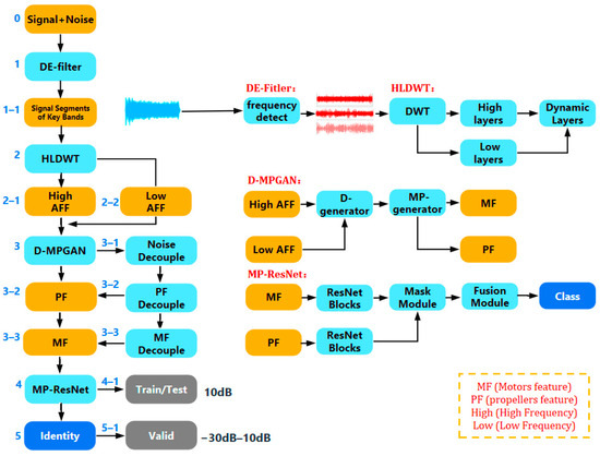
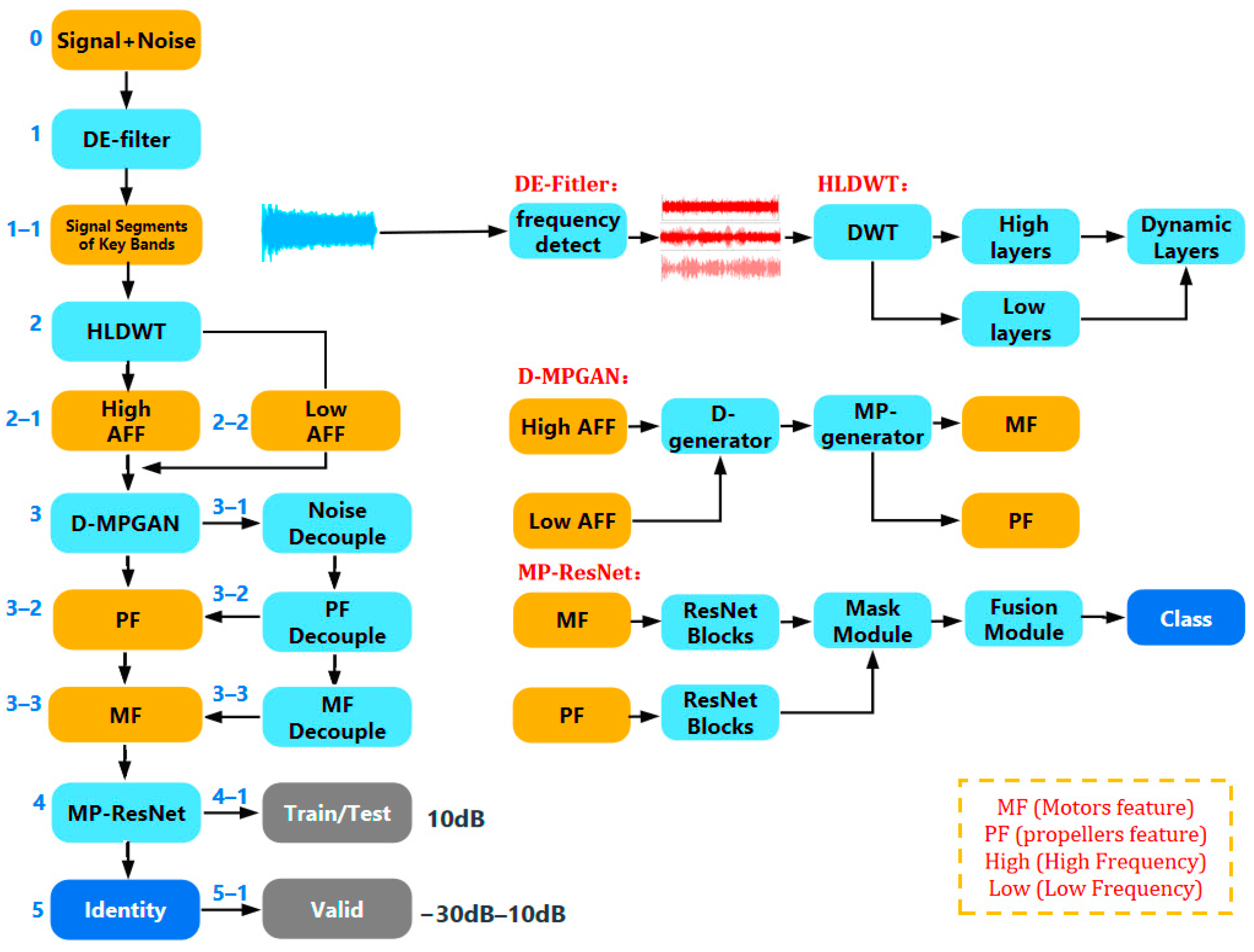
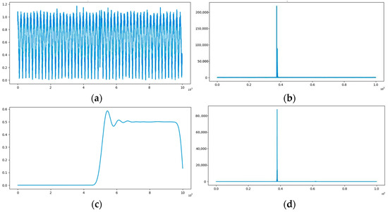
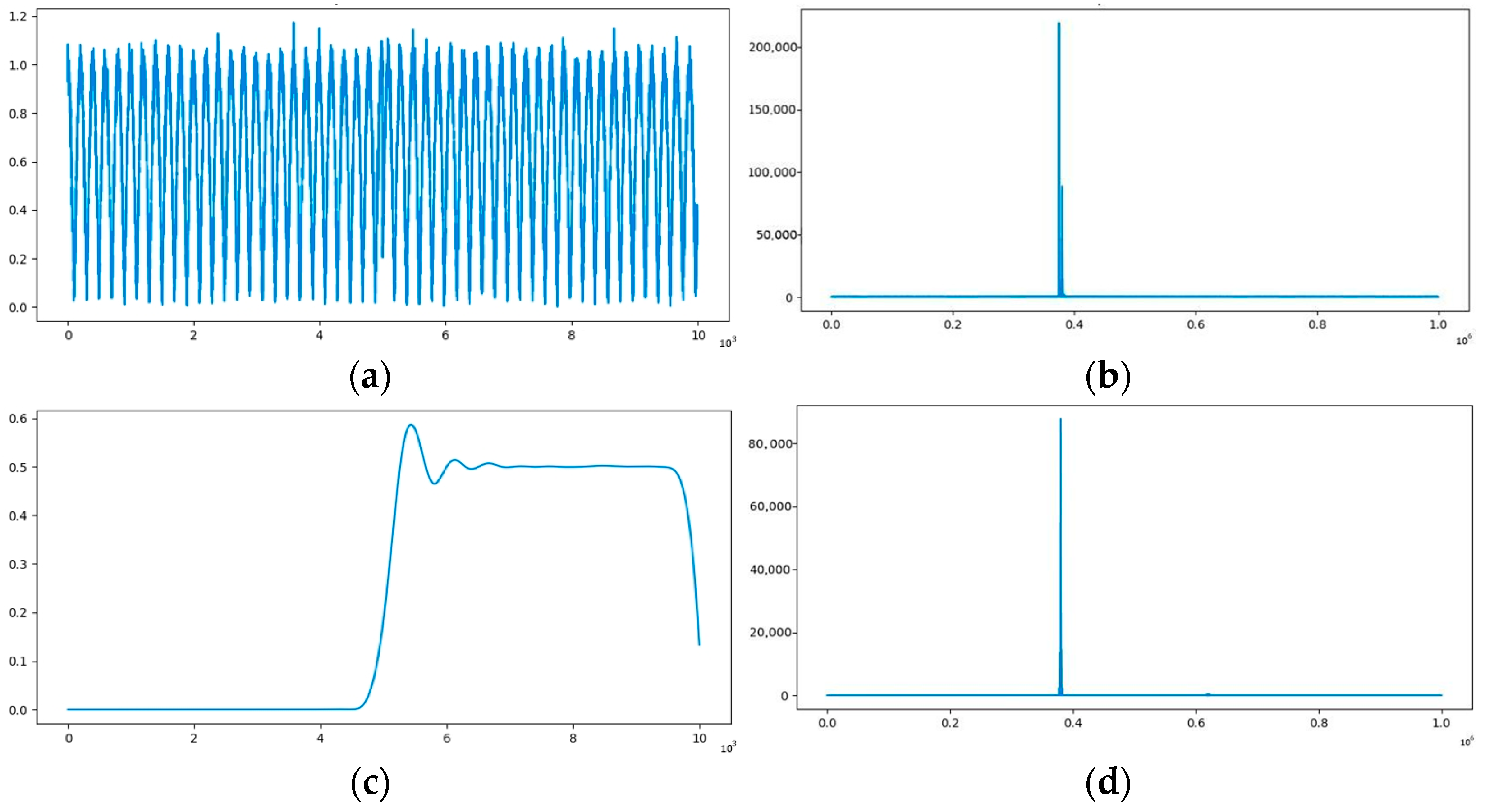




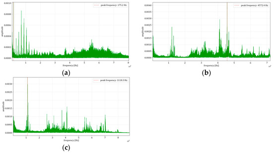
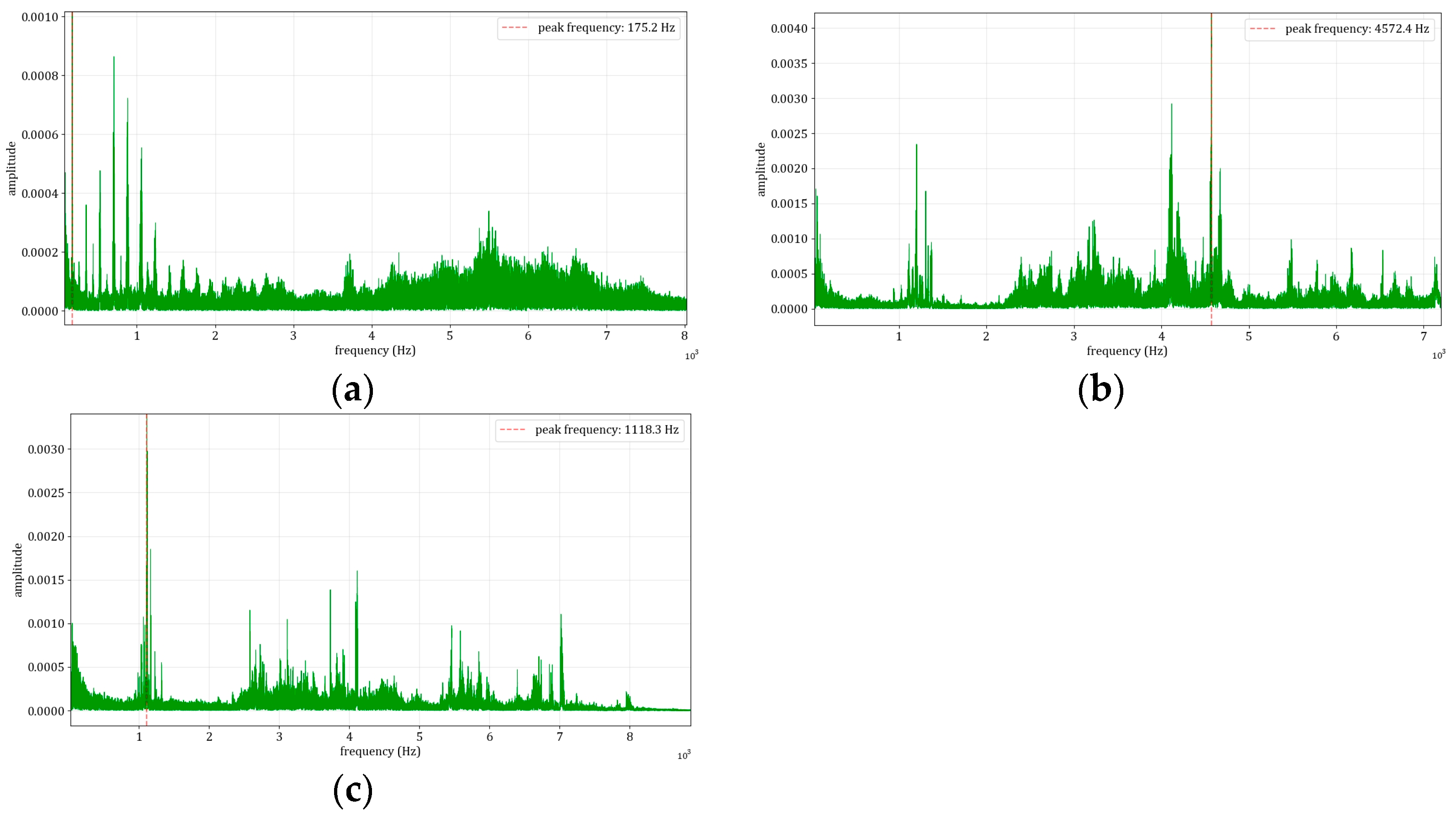
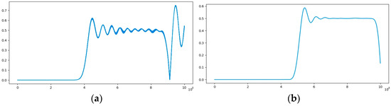
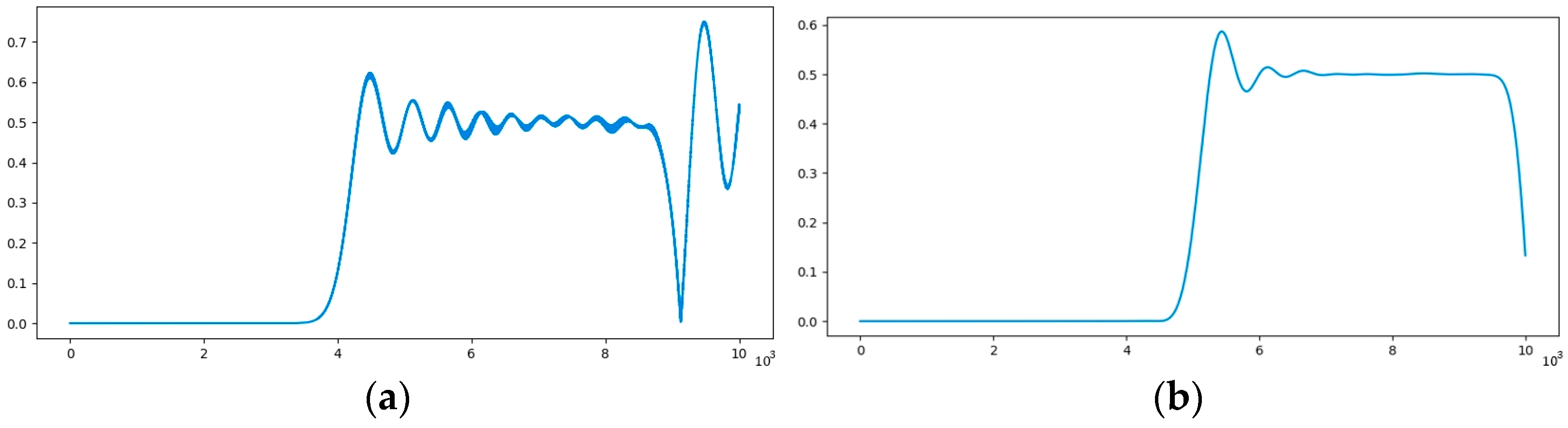
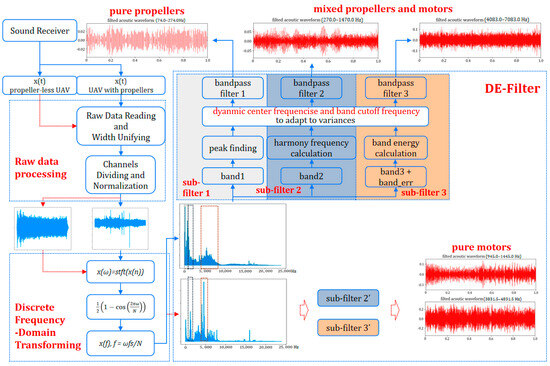
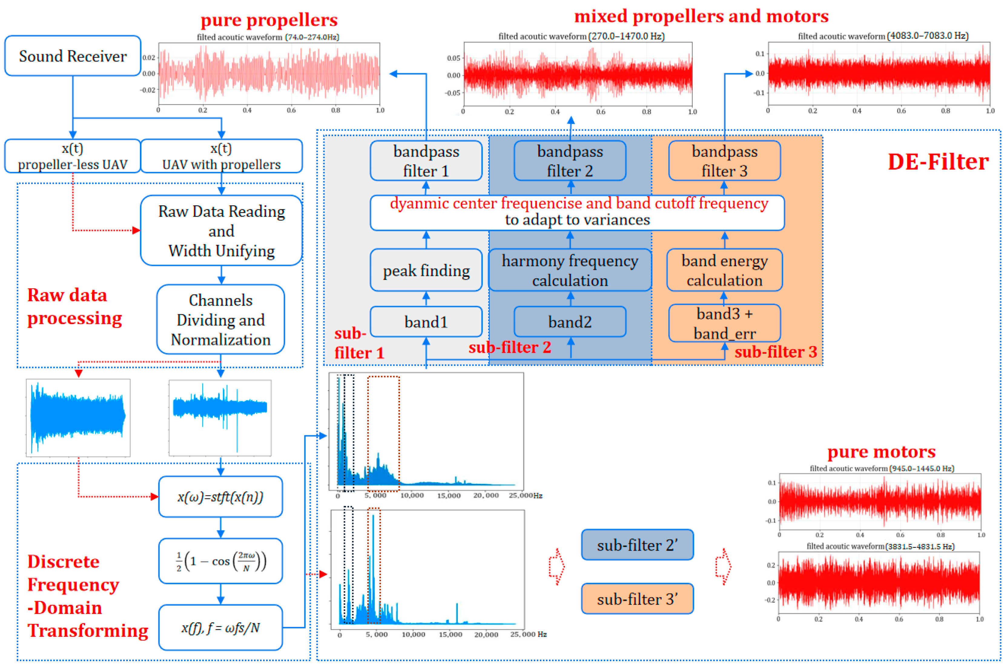
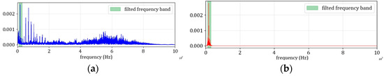
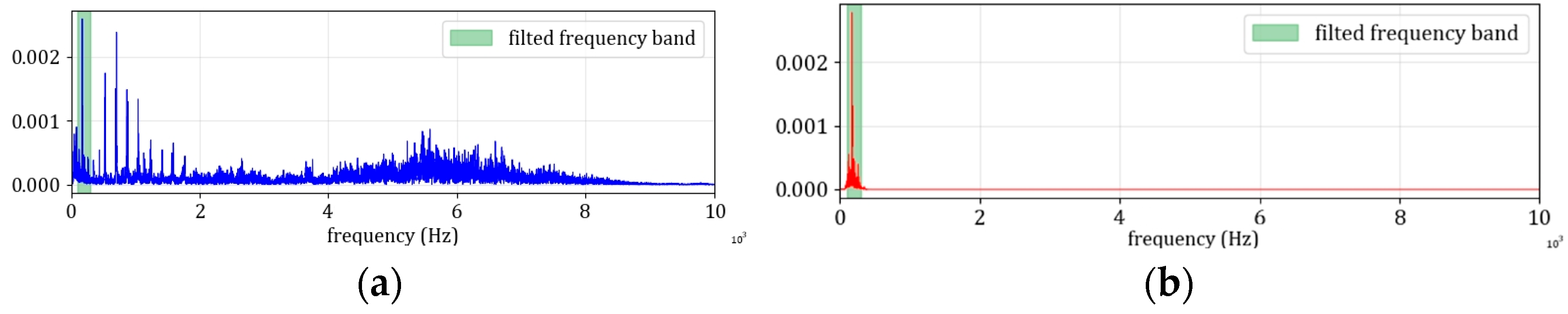
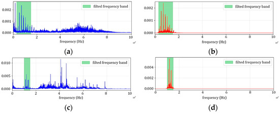
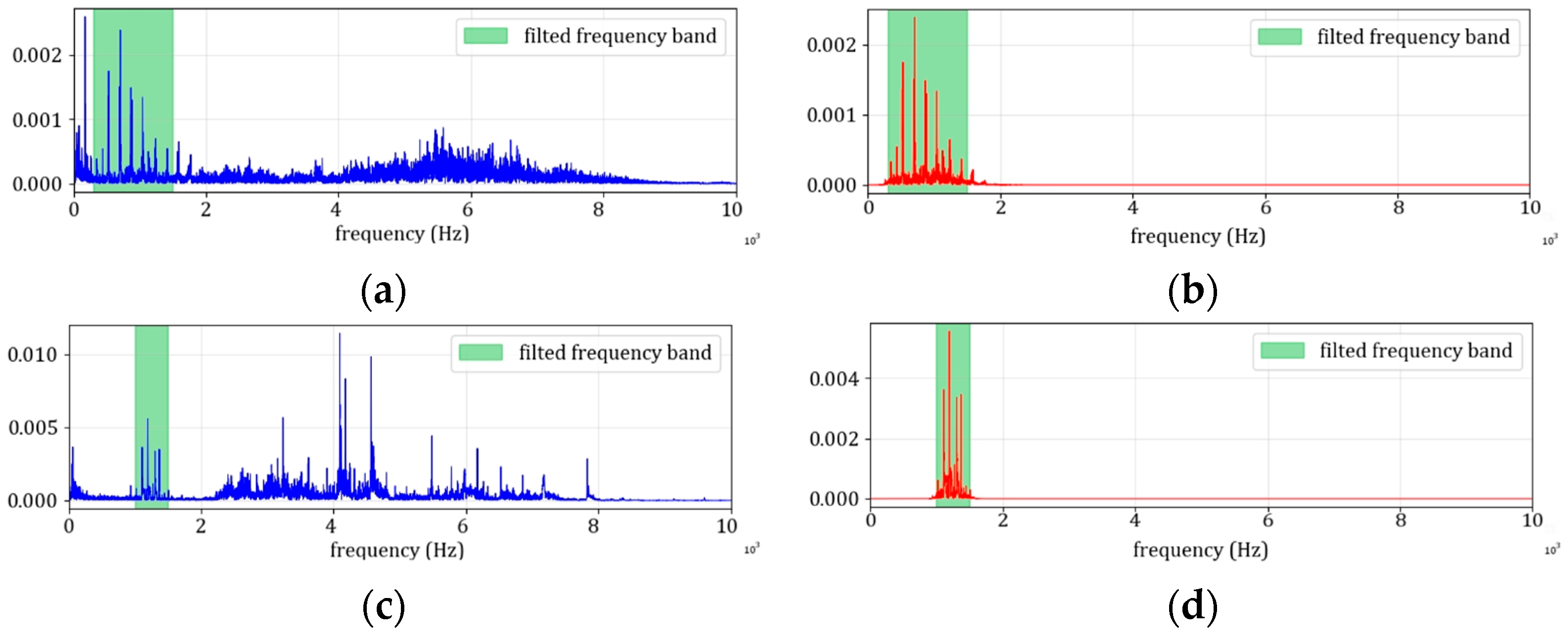
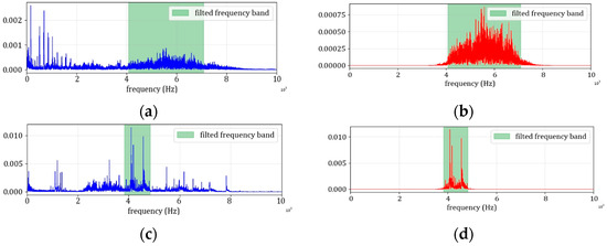
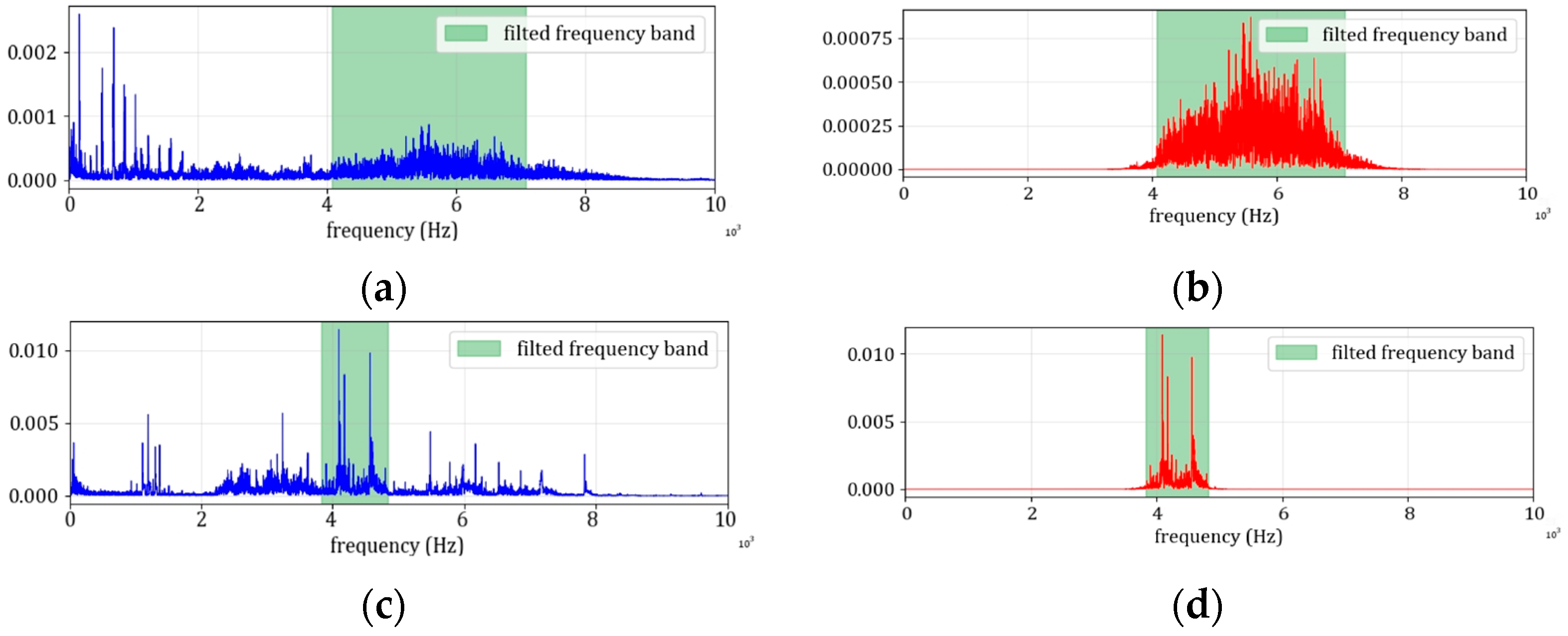
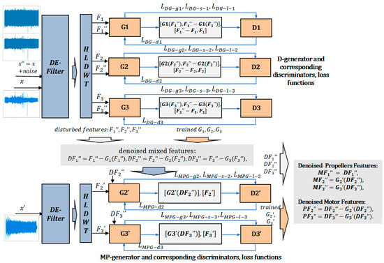
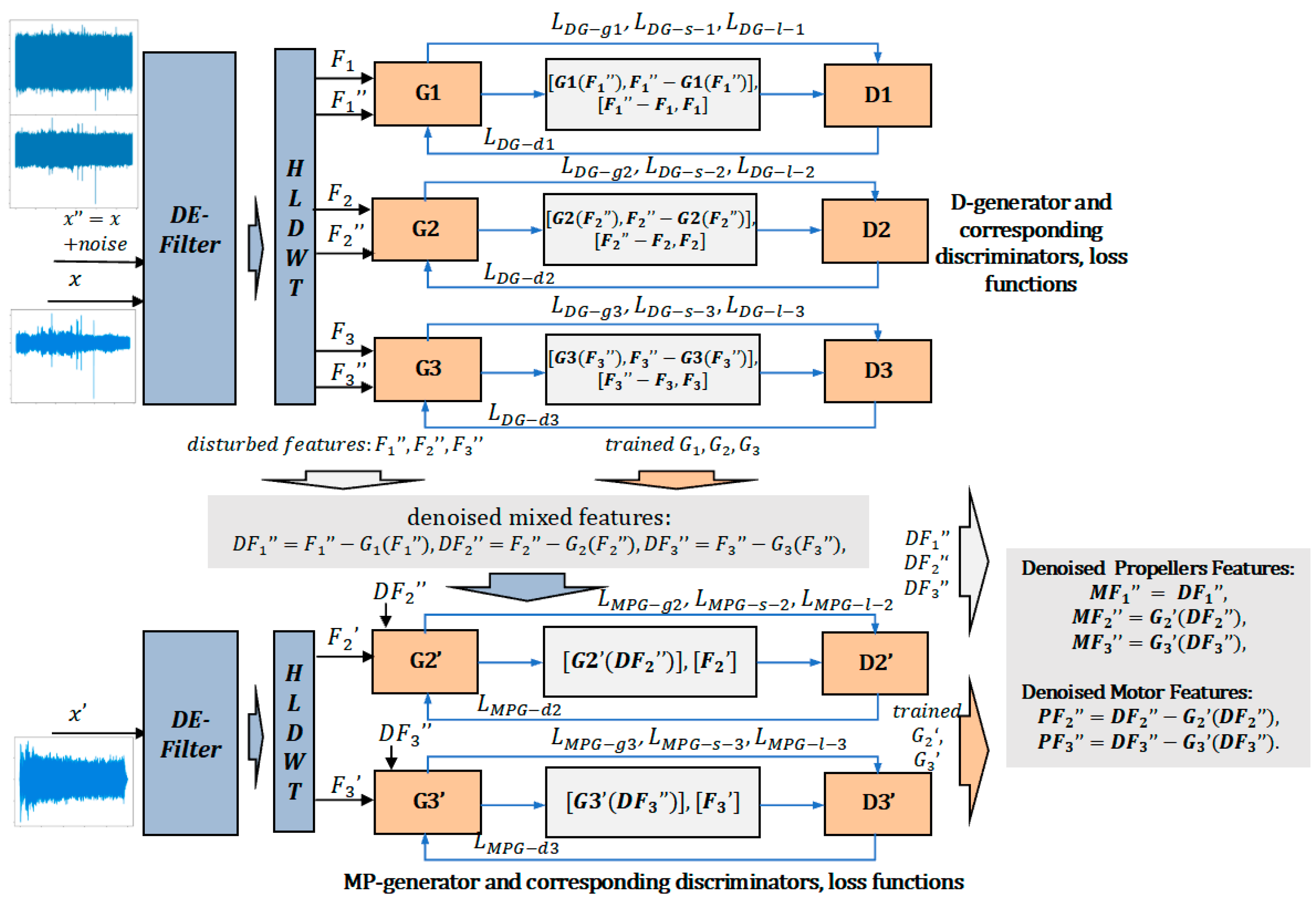
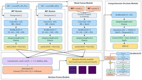
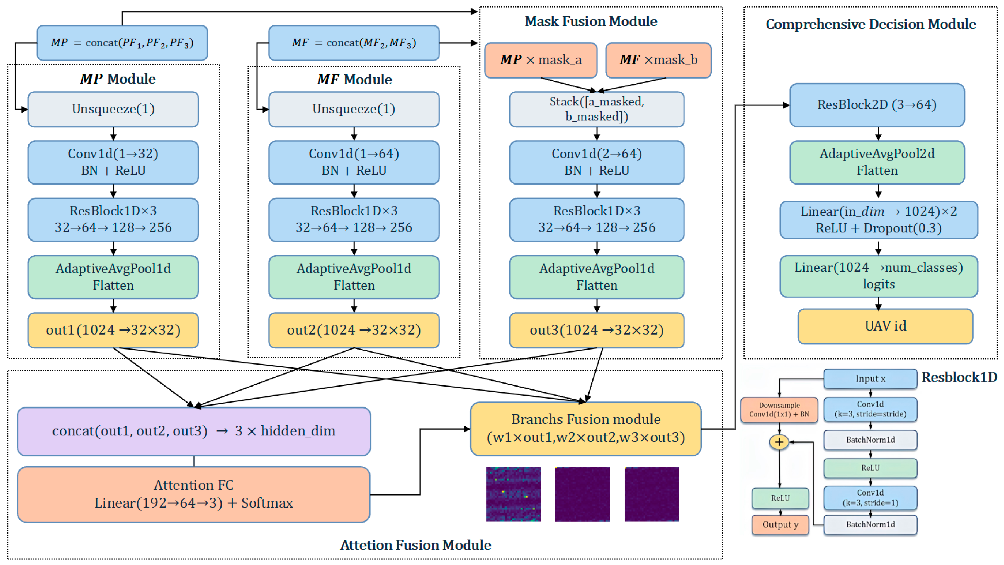
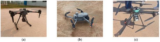
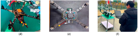
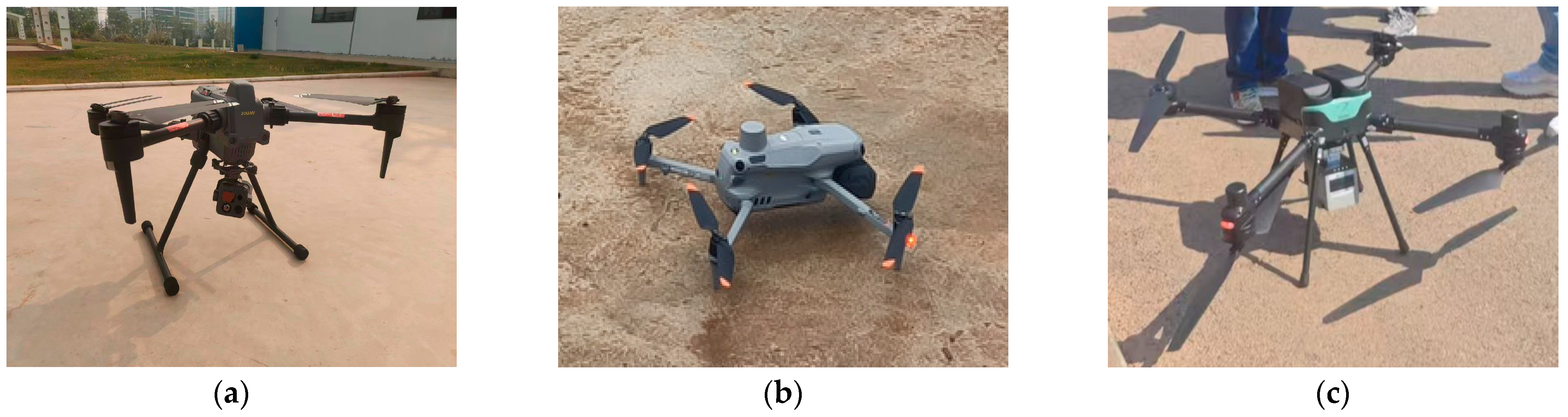
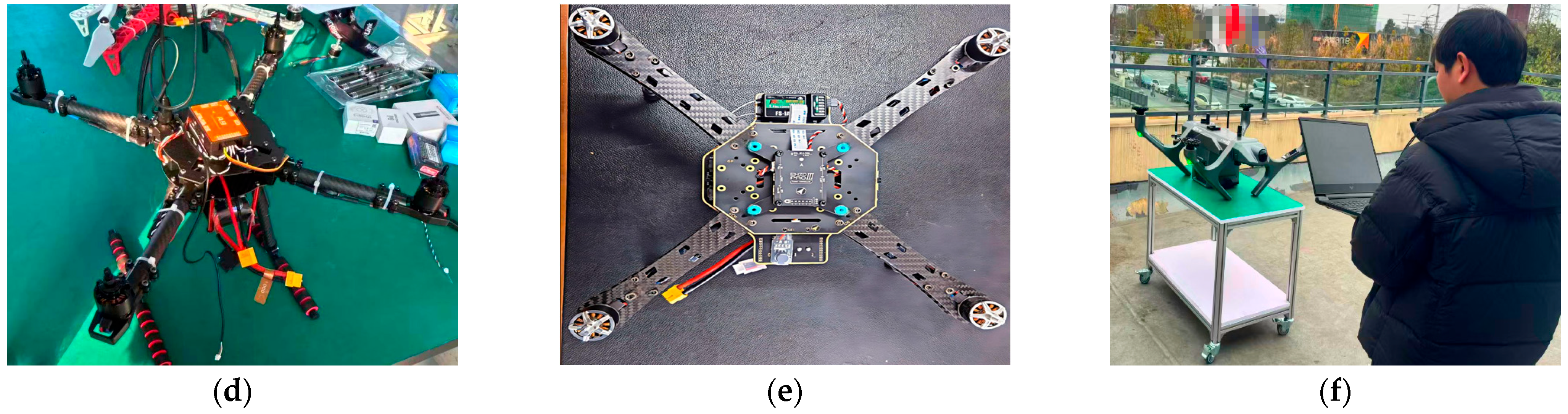
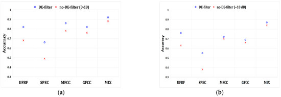
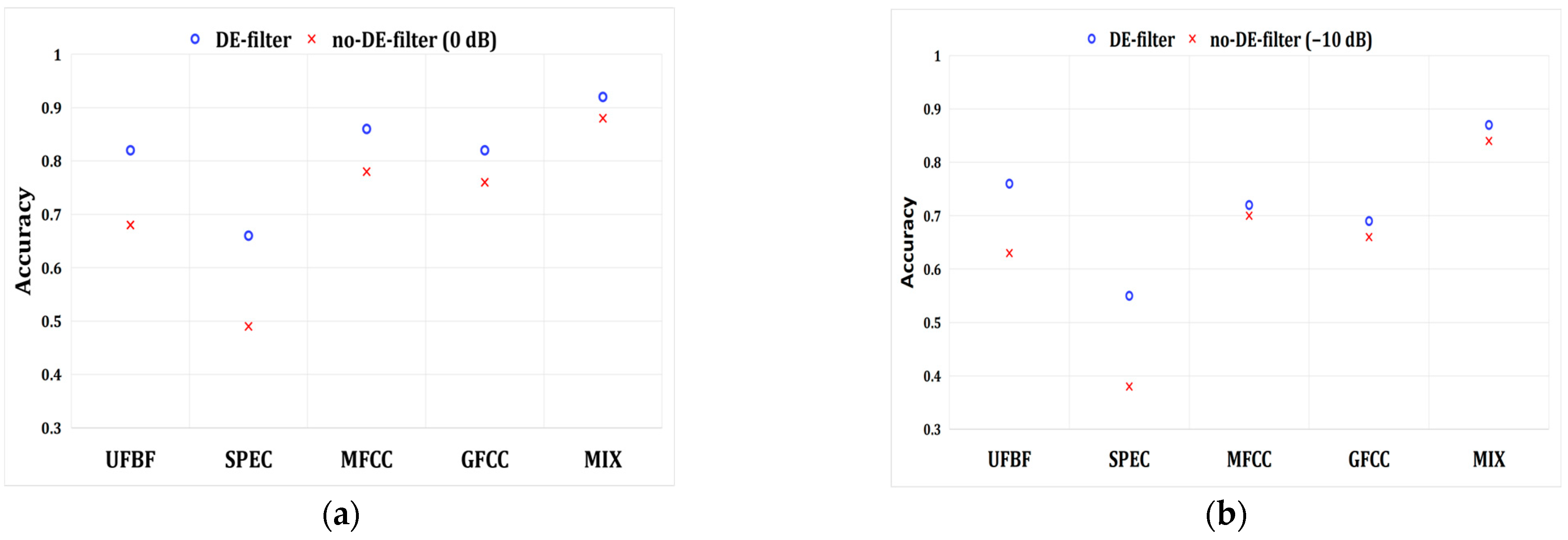
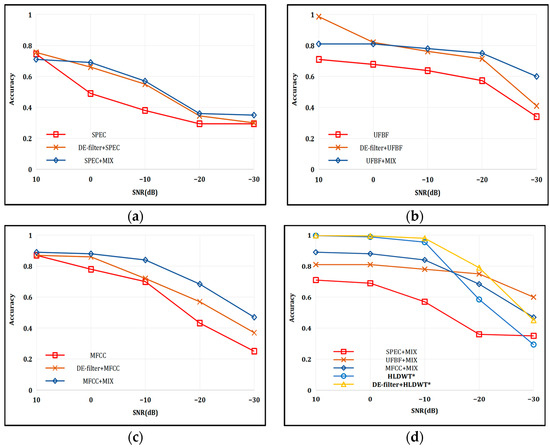
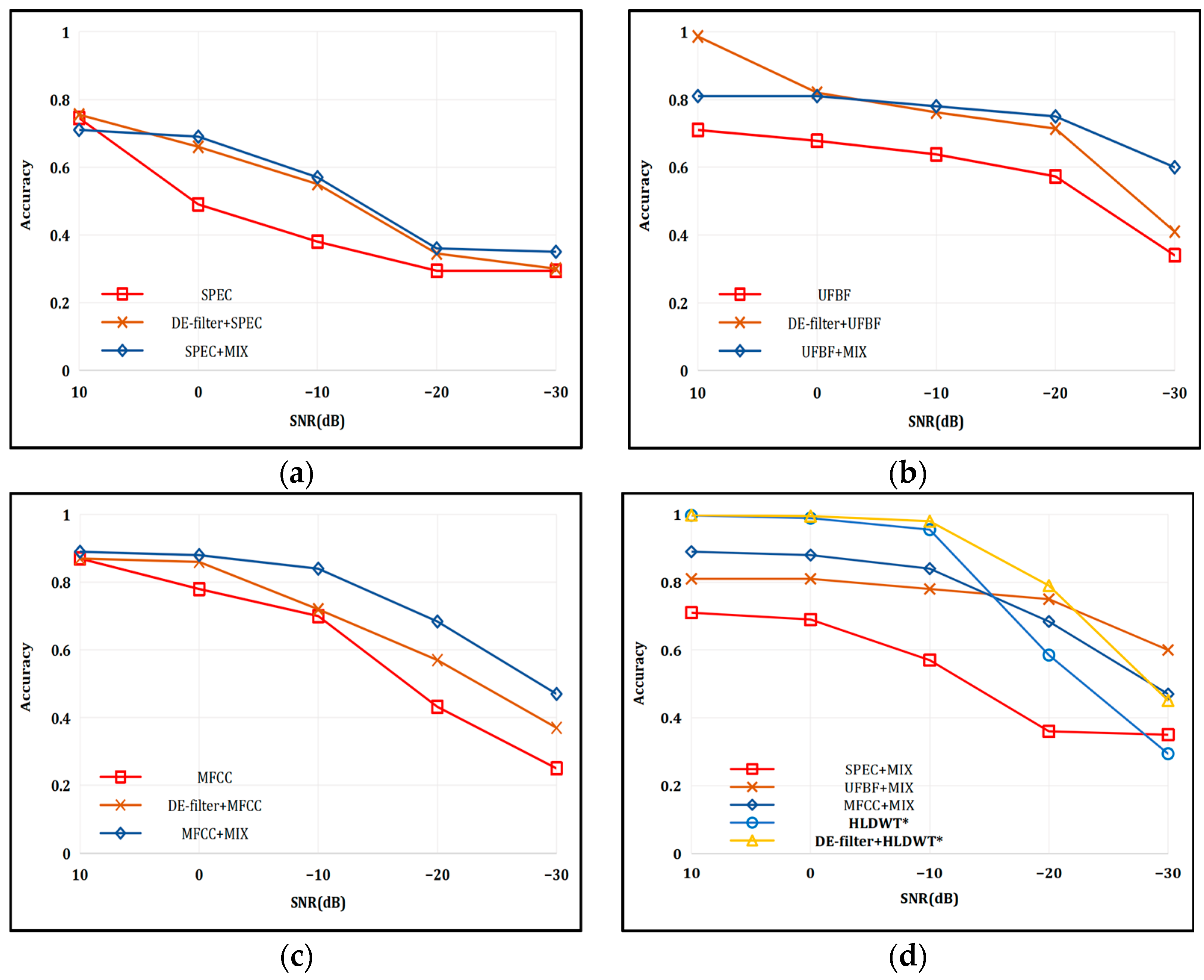
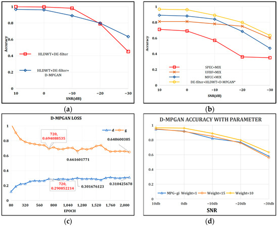
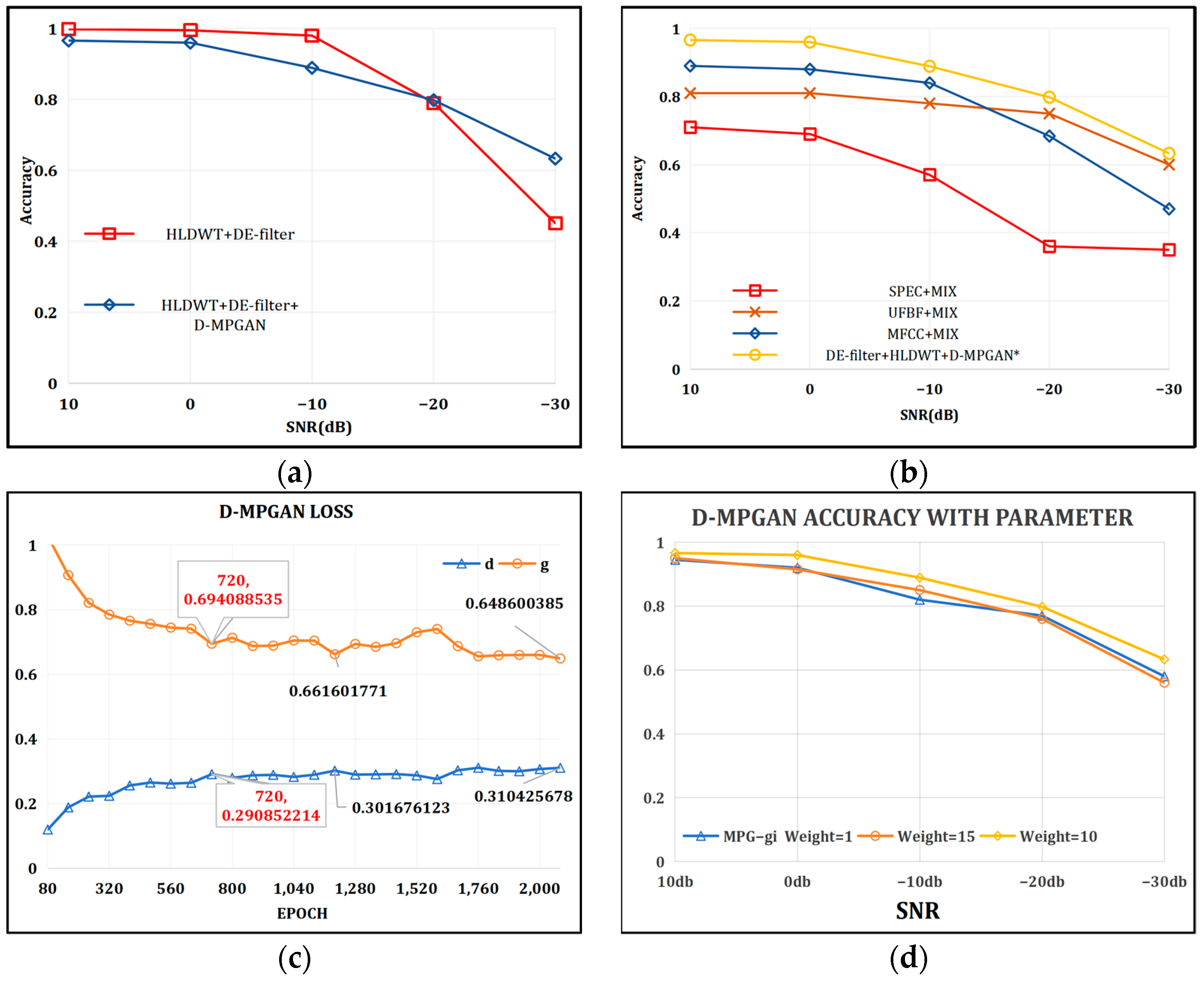
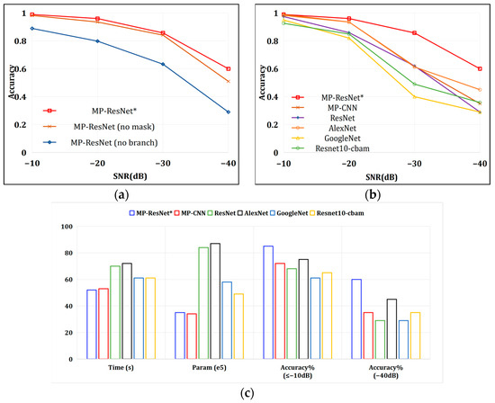
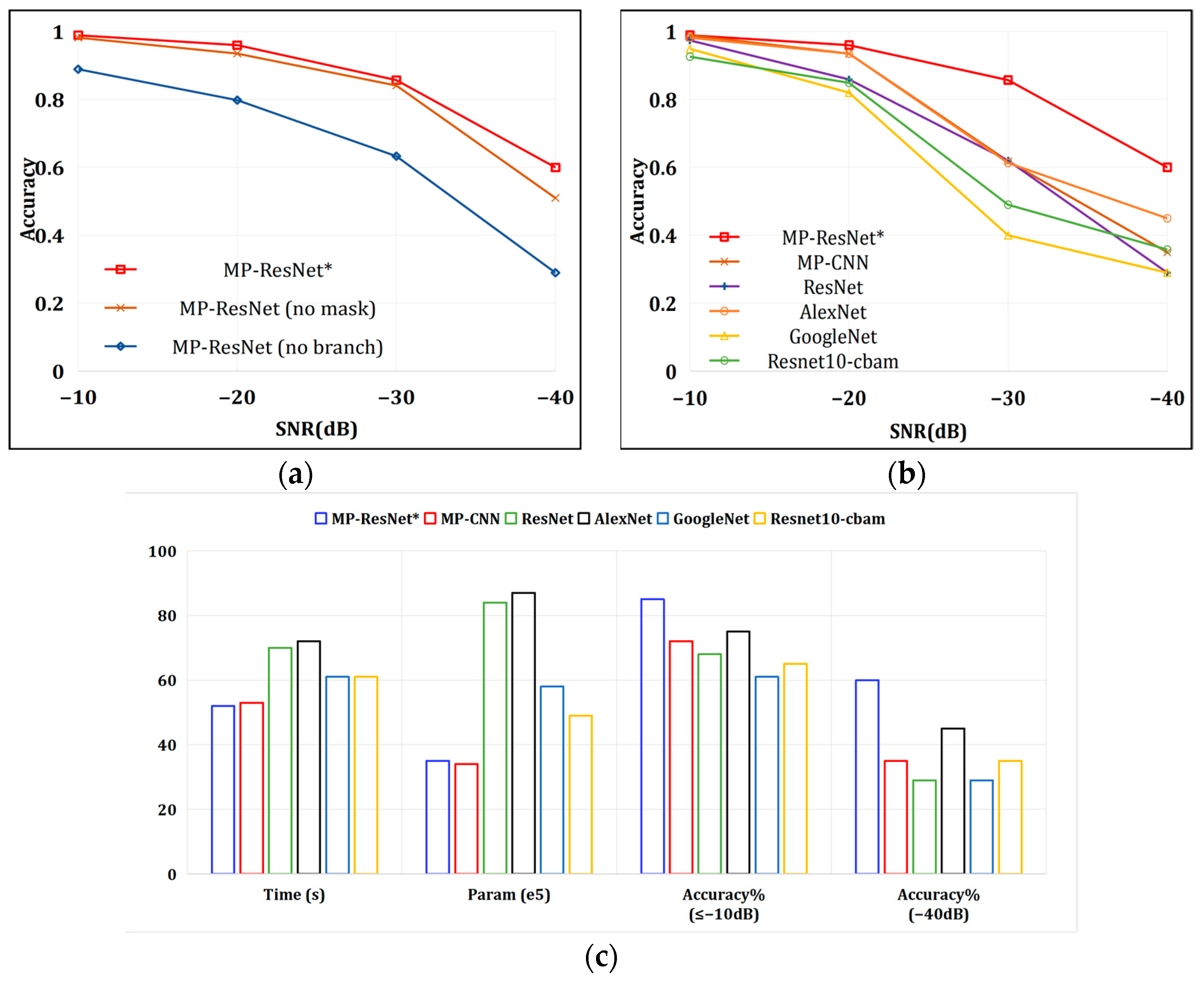

Disclaimer/Publisher’s Note: The statements, opinions and data contained in all publications are solely those of the individual author(s) and contributor(s) and not of MDPI and/or the editor(s). MDPI and/or the editor(s) disclaim responsibility for any injury to people or property resulting from any ideas, methods, instructions or products referred to in the content. |
© 2026 by the authors. Licensee MDPI, Basel, Switzerland. This article is an open access article distributed under the terms and conditions of the Creative Commons Attribution (CC BY) license.