Low-Memory Evaluation of Associated Legendre Functions for Scattered-Point Spherical Harmonic Synthesis

Abstract

In scattered-point spherical harmonic synthesis, repeated pointwise evaluation of associated Legendre functions is a major computational kernel. Recurrence methods use little memory but contain sequential degree dependence, whereas phase-function evaluators provide high accuracy using larger resident tables. We present a guarded hybrid evaluator that moves the high-accuracy reference evaluator to offline precomputation and replaces it at runtime with a compact three-dimensional Chebyshev table of smooth phase-related quantities. The surrogate path is used in numerically safe regions, and a C++ scaled recurrence with exponent tracking provides the fallback near turning points and in exponentially decaying regions. For bandlimits up to 4096, the runtime table is 3.66 MiB, about 60 times smaller than the public ALegendreEval table set used here. Across sparse scattered-point benchmarks, the method agrees with the reference evaluator at 10⁻¹¹-level output differences and achieves representative speedups of 2–5 over an optimized C++ recurrence baseline; even unfavorable cases fall back to recurrence-level runtime. These results show that reference-level Legendre evaluation can be reorganized into a low-resident-memory kernel suitable for repeated scattered-point synthesis.

1. Introduction

Accurate representation of fields on the sphere and repeated evaluation at observation or query points are essential in environmental monitoring, gravitational and magnetic field modeling, data assimilation, inverse problems, and space-borne data analysis [1,2,3,4,5,6,7]. In such applications, spherical harmonic expansions are used as standard representations because they form an orthogonal basis on the sphere, enabling fields to be represented and analyzed according to spatial scale. Practical workflows operate in both physical and coefficient spaces: states are usually stored, updated, and estimated in the latter, whereas observational comparison, physical diagnostics, navigation correction, and visualization are performed in the former. This renders repeated reconstruction based on spherical harmonic coefficients unavoidable [5,6,7,8,9,10,11]. The present study focuses on scattered-point spherical harmonic synthesis, where the evaluation points do not lie on a regular grid.

Conceptually, if a field on the sphere is represented by

$$f(\theta ,\phi )\approx \sum _{l,m}{a}_{l,m}{Y}_l^m(\theta ,\phi ),$$

(1)

then the task is to evaluate $f({\theta }_i,{\phi }_i)$ at many irregular points $({\theta }_i,{\phi }_i)$. Here, $l$ and $m$ denote the degree and order, respectively, $a_{l,m}$ denote spectral coefficients, and $({\theta }_i,{\phi }_i)$ denote angular coordinates of evaluation points. In practice, this reconstruction reduces to repeated evaluation of associated Legendre functions for many triplets $(l,m,{\theta }_i)$. Individual associated Legendre evaluations of high degree and order are already known to be computationally demanding as they require oscillation or decay, turning-point behavior, normalization, and underflow avoidance to be addressed simultaneously. For example, with $L_{\max }=4096$, a sparse mode set of size $P=128$, and $N=\mathrm{32,768}$ scattered points, 100 iterations require approximately $P\times N\times 100\approx 4.2\times {10}^8$ kernel evaluations. In addition, some accurate evaluators rely on runtime tables that must stay resident while processing many query batches. Consequently, both the runtime and resident memory footprint of associated Legendre evaluators affect the time-to-solution, concurrency, and practical deployability significantly.

On structured grids, longitudinal fast Fourier transforms and latitudinal reuse reduce repeated work [8,9,10,11,12]. At scattered points, by contrast, associated Legendre values must be generated at each distinct colatitude, with little reuse across latitude lines; the evaluator kernel therefore becomes the relevant computational unit. Existing evaluators follow two principal lines. Stable normalized recurrence schemes avoid large precomputed tables and underpin established spherical-harmonic software [9,10,13,14,15,16], but their degree-by-degree dependence can limit throughput when only sparse, noncontiguous modes are requested. Bremer and Rokhlin developed nonoscillatory phase functions for Legendre equations [17], and Bremer subsequently combined phase functions with multidimensional Chebyshev expansions for point evaluation in time independent of degree and order [18]; ALegendreEval (commit e871d16) provides a public high-accuracy implementation of this approach [19]. These phase-based methods serve as strong accuracy references, but the public implementation relies on runtime tables substantially larger than the memory budget targeted here. The resulting design question is whether phase-function accuracy can be retained over a prescribed bandlimit while replacing the reference tables by a MiB-scale runtime representation and retaining competitive throughput against grouped recurrence.

To achieve this trade-off relationship, we adopt a runtime organization where a high-accuracy reference evaluator is used during offline phases, and is not included in online runtime. To this end, smooth phase-related quantities are compressed into a three-dimensional Chebyshev coefficient table to create a phase surrogate. The turning-point neighborhood and the exponentially decaying regime are addressed using scaled recurrence with the support of exponent tracking. Our objective is not to replace a fully general evaluator for arbitrarily large degrees, but rather to cover a practically useful bandlimit (primarily $L_{\max }\lesssim 4096$ in the current implementation) and performing comparably to the reference evaluator at the ${10}^{-11}$ level with a small resident table. Our motivating implementations include repeated evaluations of spherical-harmonic geomagnetic field models in automotive, aeronautical, and maritime navigation, and batch processing of many-observation sets on ground-based systems [20,21]. These examples require arbitrary-position spherical harmonic values rather than individual structured transforms. When multiple processes, routes, trajectories, or assimilation members are evaluated concurrently, a smaller resident evaluator table directly reduces the memory budget required per worker and improves the feasibility of deployment in memory-constrained systems.

We evaluate the proposed method against two baselines. Against grouped recurrence, we measure throughput in scattered-point sparse-mode workloads. Against ALegendreEval, we evaluate agreement with a high-accuracy reference and efficiency in terms of both execution time and resident memory. To reduce contamination from language-level effects and call overhead, the recurrence baseline and the fallback recurrence in the proposed method share the same C++ kernel, so that differences can be interpreted primarily as differences between the underlying algorithms. The main technical contributions of this paper are as follows.

• We propose a method that removes the high-accuracy reference evaluator from runtime, compresses smooth quantities derived from the phase derivative into a three-dimensional Chebyshev coefficient table, and realizes a phase surrogate with MiB-scale resident memory.
• We separate the physical evanescent region from a finite protection band on the oscillatory side of the turning point, and route both regions to scaled normalized recurrence with exponent tracking. This guarded construction provides stable whole-domain coverage without requiring the phase surrogate to operate where its finite-degree approximation is most sensitive.
• We present a reproducible evaluation protocol, with fixed recurrence comparison condition ($m$-grouped shared recurrence) and memory definitions (table file size, resident table memory, and peak additional runtime memory). Thus, our conclusions do not depend on any single selected metric.

The remainder of this paper is organized as follows. The problem statement, notation, and evaluation metrics are presented in Section 2. The mathematical construction of the proposed method is presented in Section 3. The implementation of the reproducibility package is discussed in Section 4. The experimental configuration is presented in Section 5. The main results of the study are presented in Section 6. The novelty, applicability, and limitations of the study are discussed in Section 7. Finally, the paper is concluded in Section 8.

2. Problem Statement, Notation, and Evaluation Metrics

This section focuses on the (i) normalization and kernel quantity to be evaluated, (ii) scattered-point sparse-mode workload, (iii) comparison targets, and (iv) memory and performance metrics.

2.1. Angles, Degrees, and Normalization

We denote spherical coordinates by colatitude $\theta \in [0,\pi ]$ (north pole at $\theta =0$, equator at $\theta =\pi /2$) and longitude $\phi \in [0,2\pi )$. We also use $x=\cos \theta$ as an auxiliary variable. The phase surrogate is constructed using the $\theta$ coordinate because the phase function exhibits nearly linear variation with respect to $\theta$. The benchmarks considered in this paper are restricted to $\theta \in [0,\pi /2]$ (the northern hemisphere). However, this restriction does not limit the generality of the kernel evaluation as the symmetry $P_l^m(-x)=(-1{)}^{l-m}{P}_l^m(x)$ implies $K_{l,m}(\pi -\theta )=(-1{)}^{l-m}{K}_{l,m}(\theta )$. Thus, southern-hemisphere kernel values can be obtained by evaluating the mirrored northern-hemisphere angle and multiplying by $-1^{l-m}$ before applying the original longitudinal factors. Random benchmark points do not include the exact pole; in applications, pole values can be inferred based on the standard limiting forms of the associated Legendre functions. Degrees and orders satisfy $0\le m\le l\le L_{\max }$, where $L_{\max }$ denotes the bandlimit. The associated Legendre functions admit several normalization conventions; in this paper, we adopt the following fully normalized convention commonly used in spherical harmonic computation:

$${\stackrel{⃐}{P}}_l^m(x)=\sqrt{{\displaystyle \frac{2l+1}{2}}{\displaystyle \frac{(l-m)!}{(l+m)!}}}\hspace{0.17em}{P}_l^m(x).$$

(2)

We define the kernel quantity used throughout the paper as follows:

$$K_{l,m}(\theta )=\sqrt{\sin \theta }\hspace{0.17em}{\stackrel{⃐}{P}}_l^m(\cos \theta ).$$

(3)

$K_{l,m}$ are introduced to compare the proposed method, recurrence baseline, and reference evaluator for identical output quantities. As ALegendreEval returns a quantity corresponding to this kernel rather than ${\stackrel{⃐}{P}}_l^m(\cos \theta )$ itself, we adopt $K_{l,m}\left(\theta \right)$ as the common comparison target. When the full spherical harmonic value is needed, ${\stackrel{⃐}{P}}_l^m(\cos \theta )$ is recovered from $K_{l,m}$ by dividing it by $\sqrt{\sin \theta }$ away from the pole, with pole limits treated separately.

2.2. Scattered-Point Spherical Harmonic Synthesis and Sparse-Mode Workload

The target synthesis problem is reduced to the repeated pointwise evaluation of $K_{l,m}\left(\theta \right)$ when only a sparse set of modes is considered instead of the full triangular band. We adopt the following real spherical harmonic basis without the Condon–Shortley phase:

$$f(\theta ,\phi )\approx {\displaystyle \frac{1}{\sqrt{2\pi }}}{\displaystyle \sum _{l=0}^{L_{\max }}}{a}_{l,0}\hspace{0.17em}{\stackrel{⃐}{P}}_l^0(\cos \theta )+{\displaystyle \frac{1}{\sqrt{\pi }}}{\displaystyle \sum _{l=1}^{L_{\max }}}{\displaystyle \sum _{m=1}^l}{\stackrel{⃐}{P}}_l^m(\cos \theta )\hspace{0.17em}\left(a_{l,m}^{\left(c\right)}\cos (m\phi )+a_{l,m}^{\left(s\right)}\sin (m\phi )\right).$$

(4)

Here we use the real basis instead of the complex one, and the factor of $\sqrt{2}$ for $m>0$ is absorbed into the pre-factor of $1/\sqrt{\pi }$. The reduction from the real basis to the kernel formulation is described in Supplementary Note S1. The sparse-mode workload is defined using the following mode set:

$$\mathcal{P}=\left\{\right(l_k,m_k){\}}_{k=1}^P, P=|\mathcal{P}|\ll (L_{\max }+1{)}^2,$$

(5)

and repeated evaluation of

$$y({\theta }_i)={\displaystyle \sum _{k=1}^P}{a}_k\hspace{0.17em}{K}_{l_k,m_k}({\theta }_i)$$

(6)

at scattered points. Here, $a_k$ denotes the weight attached to each selected mode. In the kernel-only benchmarks, we compare direct evaluations of $K_{l,m}\left({\theta }_i\right)$, without considering weighted sums. In the end-to-end synthesis benchmark, additional coefficients and longitudinal phase factors are included.

2.3. Comparison Targets and Comparison Conditions

We consider the two following baselines.

Recurrence baseline (primary baseline for speed): This method computes $K_{l,m}\left(\theta \right)$ using normalized recurrence, without relying on a resident table. To avoid confounding algorithmic differences with trivial implementation disadvantages, the primary recurrence baseline is taken to be a grouped recurrence that shares the recurrence state across multiple $l$ values with the same $m$ value. The recurrence baseline and fallback recurrence used in the proposed method are based on the same C++ kernel; therefore, speed differences are interpreted as having been induced by structural algorithmic differences rather than language artifacts.

Reference evaluator (primary baseline for accuracy and memory): We use ALegendreEval [17,18,19], based on the Bremer phase function approach, as the reference for accuracy. Raw timing relative to the reference evaluator is treated as a secondary comparison metric to account for the variability of implementation-level effects, such as language binding and table loading. The primary comparison metrics are taken to be output agreement and reduction in resident memory; comparison in terms of memory-aware timing ratio is reported separately from that with respect to the recurrence speed.

2.4. Accuracy Metrics

Let $y^{\mathrm{ref}}$ denote the output computed by the reference evaluator and $y^{\mathrm{prop}}$ the output computed by the proposed method. In kernel-only benchmarks, $y$ denotes the stacked vector of the evaluated kernel values $K_{l,m}\left({\theta }_i\right)$ over the sampled mode–point pairs. In the end-to-end benchmark, $y$ denotes the synthesized field value after including the coefficients and longitudinal factors. We define the relative difference as follows:

$$\mathrm{reldiff}(y^{\mathrm{prop}},y^{\mathrm{ref}})={\displaystyle \frac{|y^{\mathrm{prop}}-y^{\mathrm{ref}}|}{\max \left(\right|y^{\mathrm{ref}}|,ϵ)}},$$

(7)

where we assume $ϵ={10}^{-300}$ to avoid division by zero. In this paper, we mainly report its maximum value. Within-case error distributions are visualized with the help of the case-normalized absolute error, defined as follows:

$${\mathrm{nabs}}_{\mathrm{case},i}={\displaystyle \frac{|y_i^{\mathrm{prop}}-y_i^{\mathrm{ref}}|}{\underset{j}{\max }|y_j^{\mathrm{ref}}|}}.$$

(8)

This error is used instead of pointwise relative errors as the latter become unstable near zeros of the reference solution.

2.5. Memory Metrics

The phrase “low memory” is ambiguous without a reference scale. Two metrics are used to characterize memory—the size of the evaluator table and peak additional runtime memory (RSS peak delta). The former distinguishes table file size from resident table memory after loading and the latter acts as a practical proxy for additional physical memory consumed during execution. As these quantities are fundamentally different, the two metrics are not combined into a single one.

2.6. Performance Metrics

For comparison with the recurrence baseline in terms of speed, we define speedup as follows:

$$S_{\mathrm{recur}}={\displaystyle \frac{t_{\mathrm{recur}}}{t_{\mathrm{prop}}}},$$

(9)

where $t_{\mathrm{recur}}$ and $t_{\mathrm{prop}}$ denote the runtimes of the recurrence baseline and proposed method, respectively. By definition, $S_{\mathrm{recur}}>1$ indicates that the proposed method is faster than the baseline.

We also introduce the following secondary time–memory efficiency metric:

$$F=t\times M,$$

(10)

where smaller values correspond to better performance, and the following improvement factor on this basis:

$$G={\displaystyle \frac{F_{\mathrm{ref}}}{F_{\mathrm{prop}}}}.$$

(11)

where $M$ denotes either the resident table memory or RSS peak delta. This metric is introduced to serve as a compact indicator to reward methods that reduce memory demands as well as runtime simultaneously. It is used only as a supporting metric; the paper also reports speed, memory, and accuracy separately to ensure that the conclusion does not depend on a single composite quantity.

3. Proposed Method: Reference-Based Phase Surrogate and Guarded Hybrid Evaluator

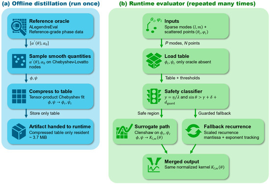
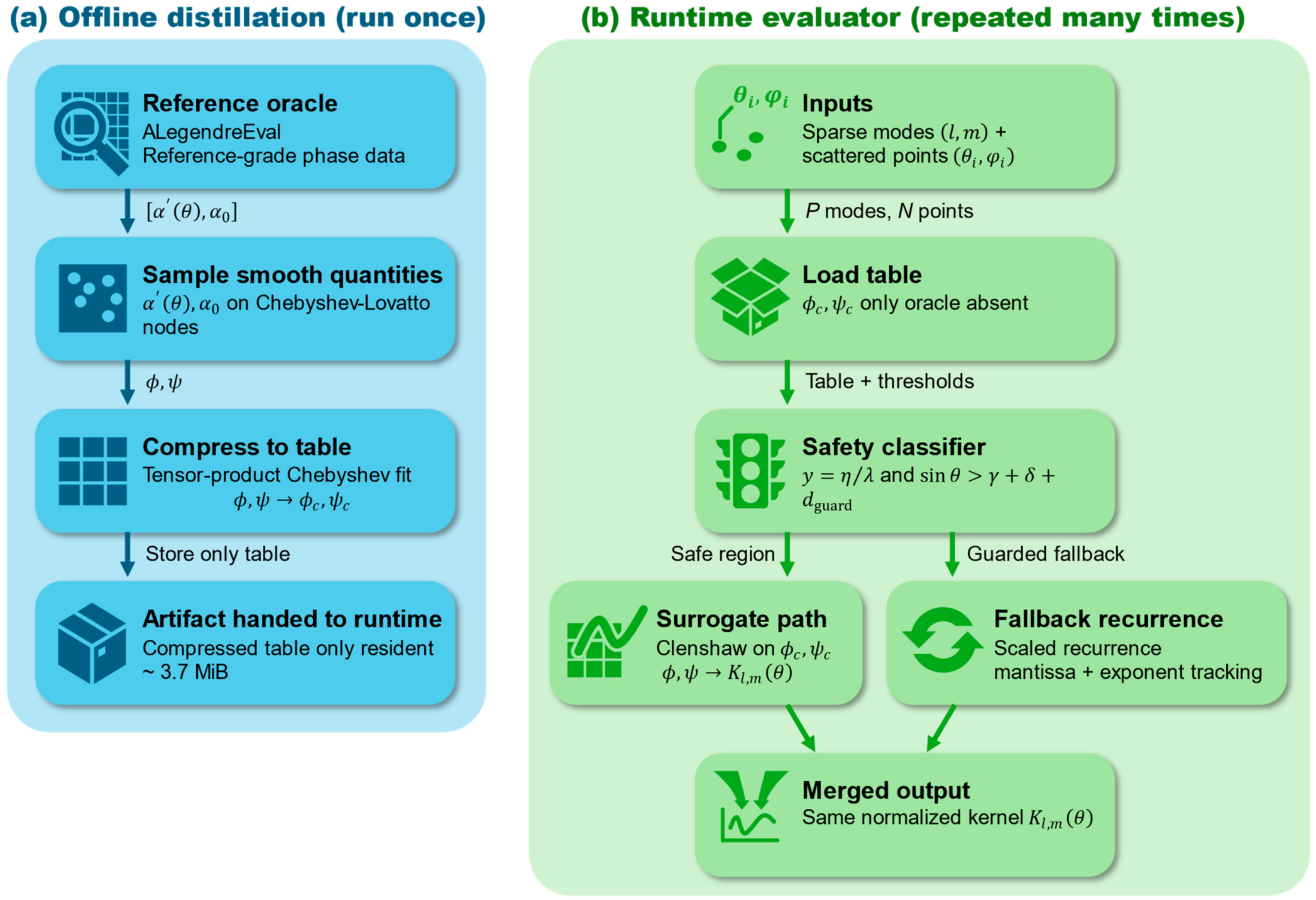
The overall structure is illustrated in Figure 1. In the offline stage, phase-derivative samples obtained from the reference evaluator are compressed into three-dimensional Chebyshev coefficient tables. At runtime, only the compressed table is loaded, and each triplet $(l,m,\theta )$ is routed either to the surrogate or scaled recurrence by a safety test.

Figure 1. Offline and runtime workflow of the proposed evaluator. The offline stage converts reference phase-derived samples into compact Chebyshev coefficient tables. At runtime, a two-stage classifier routes each query to the phase surrogate or scaled recurrence and merges the resulting values; the reference evaluator is not loaded. Panel (a) shows the one-time offline distillation, and panel (b) shows the repeatedly executed runtime evaluator.

3.1. Essentials of the Phase-Function Representation and Turning-Point Structure

Instead of approximating the highly oscillatory kernel directly, the phase-function approach approximates the phase that generates the oscillation and its derivative. This distinction is computationally fundamental: over an oscillatory interval with appreciable amplitude, the number of sign changes in the associated Legendre kernel grows with degree, so a global polynomial that resolves the kernel directly requires increasing degree as the oscillation count grows. The normalized phase quantities, by contrast, vary smoothly, while the cosine factor reconstructs the rapid oscillations analytically. The coefficient table therefore represents smooth generator functions rather than storing the oscillations themselves.

The kernel $K_{l,m}(\theta )=\sqrt{\sin \theta }\hspace{0.17em}{\stackrel{⃐}{P}}_l^m(\cos \theta )$ satisfies the normal-form second-order ordinary differential equation:

$$K^{″}(\theta )+\left[{\lambda }^2-{\displaystyle \frac{{\eta }^2}{{\sin }^2 \theta }}\right]K(\theta )=0,$$

(12)

where $\lambda =l+1/2$ and $\eta =\sqrt{m^2-1/4}$ [17,18]. The bracketed coefficient corresponds to the square of the local wavenumber; it is positive when $\sin \theta >\gamma =\eta /\lambda$ and negative otherwise. The point $\sin \theta =\gamma$ represents the turning point ${\theta }_t=\arcsin \gamma$. The region $\sin \theta >\gamma$ is defined to be oscillatory, while the region $\sin \theta <\gamma$ is referred to as evanescent. In the implementation, we introduce a small offset $\delta >0$ away from the turning point and an additional guard width $d_{\mathrm{guard}}>0$ on the safe side. The region partition of the proposed method is defined based on this structure.

The physical and computational boundaries are distinct. The physical turning point is defined by sin(theta) = gamma. The tabulation offset delta excludes the immediate neighborhood of this point from the fitted coordinate domain, and d_guard adds a further runtime safety margin on the oscillatory side. Section 3.3 states the resulting mode-level and point-level tests explicitly.

In the Bremer phase function framework, two normalized solutions $p$ and $q$ of the associated Legendre equation are expressed as follows:

$$p\left(\theta \right)=A\left(\theta \right)\cos \left(\alpha \right(\theta \left)\right), q\left(\theta \right)=-A\left(\theta \right)\sin \left(\alpha \right(\theta \left)\right).$$

(13)

The Wronskian is assumed to be the constant $W=(2l+1)/\pi$ [17,18], and the phase derivative satisfies:

$${\alpha }^{\prime }(\theta )={\displaystyle \frac{W}{A(\theta {)}^2}}.$$

(14)

Hence,

$$A(\theta )=\sqrt{{\displaystyle \frac{2l+1}{\pi \hspace{0.17em}{\alpha }^{\prime }\left(\theta \right)}}},$$

(15)

and the kernel returned by ALegendreEval can be expressed as follows:

$$K_{l,m}(\theta )=p(\theta )=\sqrt{{\displaystyle \frac{2l+1}{\pi }}}\hspace{0.17em}{\displaystyle \frac{\cos \left({\alpha }_{l,m}\right(\theta \left)\right)}{\sqrt{{{\alpha }^{\prime }}_{l,m}\left(\theta \right)}}}.$$

(16)

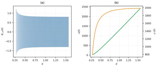
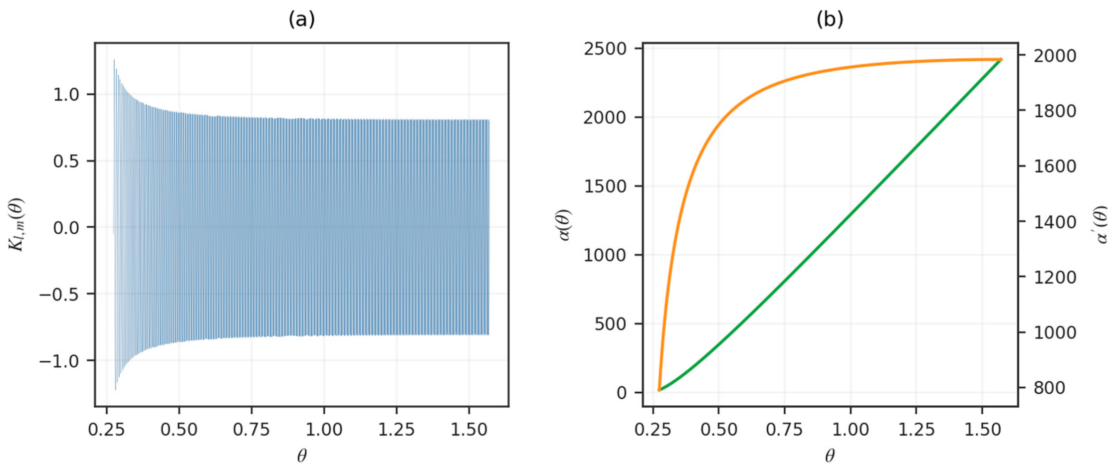
Even when $K_{l,m}$ oscillates strongly, $\alpha$ and ${\alpha }^{\prime }$ remain smooth in the oscillatory region. Figure 2 illustrates this phenomenon for $(l,m)=(2048,512)$: (a) depicts the strong oscillation of $K$, and (b) depicts the smooth variation of $\alpha$ and ${\alpha }^{\prime }$. Therefore, the surrogate is applied only in the safe oscillatory region; whereas, recurrence is used elsewhere.

Figure 2. Kernel and phase quantities for (l, m) = (2048, 512) over the surrogate-safe interval with d_guard = 0.02. (a) Oscillatory kernel K_l,m(theta). (b) Phase alpha(theta), left axis, and phase derivative alpha’(theta), right axis. The blue curve denotes the kernel, the orange curve denotes the phase on the left axis, and the green curve denotes the phase derivative on the right axis.

3.2. Reference-Based Tabulation: Three-Dimensional Chebyshev Coefficients for $\varphi$ and $\psi$

The core innovation of the proposed method lies in its removal of the reference phase function evaluator from runtime and the compression of data corresponding to only the required smooth quantities into a small table. Notably, the table does not store the values of the oscillatory kernel itself. Instead, it stores the coefficients of two slowly varying functions that generate the kernel using a phase formula. At runtime, these two functions are reconstructed based on the coefficient table, and the oscillatory behavior is recovered analytically using the cosine factor given by Equation (19).

We define

$$\lambda =l+{\displaystyle \frac{1}{2}}, \eta =\sqrt{m^2-{\displaystyle \frac{1}{4}}}, \gamma ={\displaystyle \frac{\eta }{\lambda }},$$

(17)

For m ≥ 1, gamma is real and provides a normalized order-to-degree coordinate. For m = 0, eta is imaginary under this parameterization, so the surrogate is not used.

The runtime mode-level classifier routes a complete mode to recurrence when m = 0, when gamma is below gamma_min, or when l is below the threshold l_0(m; gamma_max) defined by Equation (30). All other modes are surrogate candidates; their individual points are classified by the safety test in Section 3.3.

Using the reference phase at the equator, ${\alpha }_0={\alpha }_{l,m}(\pi /2)$, we define the two following normalized functions:

$${\varphi }_{l,m}(\theta )={\displaystyle \frac{{\alpha }_{l,m}\left(\theta \right)-{\alpha }_{l,m}(\pi /2)}{\lambda }}, {\psi }_{l,m}(\theta )={\displaystyle \frac{{{\alpha }^{\prime }}_{l,m}\left(\theta \right)}{\lambda }}.$$

(18)

The first, $\varphi$, represents the phase increment from the equator divided by the large scale factor $\lambda$; and the second, $\psi$, represents the phase derivative divided by the same factor. This scaling eliminates degree dependence to a large extent. Subsequently, the kernel is reconstructed as follows:

$$K_{l,m}(\theta )\approx \sqrt{{\displaystyle \frac{2l+1}{\pi }}}\hspace{0.17em}{\displaystyle \frac{\cos \left({\alpha }_0+\lambda \hspace{0.17em}\varphi \left(\theta \right)\right)}{\sqrt{\lambda \hspace{0.17em}\psi \left(\theta \right)}}}.$$

(19)

Since $d\varphi /d\theta =\psi$ and $\varphi (\pi /2)=0$, we have:

$${\varphi }_{l,m}(\theta )={\int }_{\pi /2}^{\theta }{\psi }_{l,m}(\xi )\hspace{0.17em}d\xi .$$

(20)

Thus, $\psi$ is obtained directly from the reference evaluator via ${\alpha }^{\prime }/\lambda$, and $\varphi$ is reconstructed by integration. The additive phase constant must also be explicitly fixed. We adopt:

$${\alpha }_0(l,m)\equiv (l-m){\displaystyle \frac{\pi }{2}}\hspace{0.25em}(\mathrm{mod}\hspace{0.25em}2\pi ),$$

(21)

which is consistent with both the parity structure of $P_l^m\left(0\right)$ [22] and the phase convention used in ALegendreEval [19]. This enables the processing of the phase constant without relying on a large additional runtime table.

The table is constructed on normalized coordinates, instead of the discrete integer lattice $(l,m,\theta )$. This enables one coefficient table to serve several integer degrees and orders. We use $\theta \in [0,\pi /2]$ as the basic domain and define the following:

Degree direction:

$$\tau ={\displaystyle \frac{1}{\lambda }}, \widehat{\tau }={\displaystyle \frac{2\tau -({\tau }_{\min }+{\tau }_{\max })}{{\tau }_{\max }-{\tau }_{\min }}}\in [-1,1];$$

(22)

Order-ratio direction:

$$\widehat{g}={\displaystyle \frac{2\gamma }{{\gamma }_{\max }}}-1\in [-1,1];$$

(23)

$\theta$ direction: with $t_{\min }=\arcsin (\gamma +\delta )$,

$$u=\sqrt{{\displaystyle \frac{\theta -t_{\min }}{\pi /2-t_{\min }}}}, \widehat{z}=2u-1\in [-1,1].$$

(24)

The square-root mapping focuses on the resolution near the turning point. Offline sampling uses Chebyshev–Lobatto nodes in $(\widehat{\tau },\widehat{g},\widehat{z})$, which are mapped back to continuous parameters $({\lambda }_i,{\gamma }_j,{\theta }_{ijk})$, and finally to

$${\nu }_i={\lambda }_i-{\displaystyle \frac{1}{2}}, {\mu }_{ij}=\sqrt{({\gamma }_j{\lambda }_i{)}^2+{\displaystyle \frac{1}{4}}}.$$

(25)

The reference evaluator is queried at continuous admissible parameters $({\nu }_i,{\mu }_{ij},{\theta }_{ijk})$; integer rounding is never used during offline sampling. These continuous parameters are only used to fit smooth surfaces in the offline stage. Runtime queries retain the original integer pairs $(l,m)$, which are mapped to normalized coordinates and evaluated via interpolation using the Chebyshev representation. On the tensor-product domain, we approximate $\varphi$ and $\psi$ using first-kind Chebyshev polynomials:

$$\varphi (\widehat{\tau },\widehat{g},\widehat{z})\approx {\displaystyle \sum _{i=0}^{p_{\tau }}}{\displaystyle \sum _{j=0}^{p_g}}{\displaystyle \sum _{k=0}^{p_z}}{c}_{i,j,k}^{\varphi }\hspace{0.17em}{T}_i(\widehat{\tau })\hspace{0.17em}{T}_j(\widehat{g})\hspace{0.17em}{T}_k(\widehat{z}),$$

(26)

and similarly for $\psi$. In the implementation, $\psi ={\alpha }^{\prime }/\lambda$ is sampled first, followed by the reconstruction of $\varphi$ via spectral integration along the $\widehat{z}$ direction. The two coefficient tensors are stored separately. In practical terms, a dense table of function values over $(l,m,\theta )$ is not maintained during runtime. Only the coefficient tensors needed to reconstruct $\varphi$ and $\psi$ on demand are retained. Memory reduction is achieved by replacing as many oscillatory function samples as possible with a small set of polynomial coefficients for smooth generator functions.

3.3. Guarded Hybrid Evaluator

The runtime classifier applies two successive tests. The mode-level test first excludes m = 0, gamma < gamma_min, and l < l_0(m; gamma_max), in which case the entire mode is evaluated by recurrence. For every remaining surrogate-candidate mode, the point-level test defines the surrogate region as follows:

$${\mathsf{\Omega }}_{\mathrm{sur}}=\{\hspace{0.17em}\theta :\sin \theta >\gamma +\delta +d_{\mathrm{guard}}\hspace{0.17em}\}.$$

(27)

The two margins have distinct roles: delta is the offset used to start the tabulated oscillatory coordinate, whereas d_guard is an additional runtime safety margin. Points outside the surrogate region are evaluated by recurrence and are partitioned for interpretation as follows:

• Turning-point protection region:

$${\mathsf{\Omega }}_{\mathrm{turn}}=\{\gamma <\sin \theta \le \gamma +\delta +d_{\mathrm{guard}}\},$$

(28)

• Physical evanescent region:

$${\mathsf{\Omega }}_{\mathrm{eva}}=\{\sin \theta \le \gamma \}.$$

(29)

For a surrogate-candidate mode, the recurrence region is the union of the physical evanescent region and the turning-point protection region. The latter lies on the oscillatory side but is deliberately protected. As the turning point is approached, the local wavenumber tends to zero and the reconstructed kernel becomes increasingly sensitive to errors in the phase derivative; the first-order relation in Equation (38) contains a term proportional to (alpha’)^(−3/2). The concern is therefore the conditioning of the finite-degree surrogate reconstruction, not a singularity of the exact associated Legendre solution. At the mode level, gamma_max is enforced through the following lower-degree threshold:

$$l_0(m;{\gamma }_{\max })=\max \left(l_{\min },\hspace{0.17em}m,\hspace{0.17em}⌈{\displaystyle \frac{\eta }{{\gamma }_{\max }}}-{\displaystyle \frac{1}{2}}⌉\right),$$

(30)

Modes satisfying l < l_0(m; gamma_max) are evaluated entirely by recurrence. Equations (27)–(30) and Algorithm 1 therefore specify the same two-stage routing rule without an empirical, case-by-case decision at runtime.

Algorithm 1. Runtime Guarded Hybrid Evaluator for Scattered Points and Sparse Modes

Input: mode_set = {(l_k, m_k)}_{k = 1,…,P}; points theta [1,…,N]; coefficient tensors phi_c and psi_c; parameters l_min, gamma_min, gamma_max, delta, and d_guard Output: y[k,i] = K_{l_k,m_k}(theta_i) for (l, m) in mode_set:   lambda <- l + 1/2   if m == 0:     y[l,m,:] <- scaled_recurrence(l, m, theta)     continue   eta <- sqrt(m^2 - 1/4)   gamma <- eta/lambda   if gamma < gamma_min or l < l_0(m; gamma_max):     y[l,m,:] <- scaled_recurrence(l, m, theta)     continue   mask_sur <- sin(theta) > gamma + delta + d_guard   y_sur <- surrogate_fused(phi_c, psi_c, l, m, theta[mask_sur])   y_rec <- scaled_recurrence(l, m, theta[not mask_sur])   y[l,m,:] <- merge(mask_sur, y_sur, y_rec) return y

3.4. Scaled Normalized Recurrence with Exponent Tracking

In the evanescent region, even normalized recurrence can exhibit underflow when the order is high. Both the recurrence baseline and fallback path of the proposed method generate identical fully normalized outputs:

$$Q_l^m\left(x\right)={\stackrel{⃐}{P}}_l^m\left(x\right), x=\cos \theta ,$$

(31)

which is converted as follows:

$$K_{l,m}\left(\theta \right)=\sqrt{\sin \theta }\hspace{0.17em}{Q}_l^m(\cos \theta ).$$

(32)

Recurrence itself follows the fully normalized three-term relation reported by Holmes and Featherstone [13]; the full formulae are provided in Supplementary Note S2.

To mitigate underflow, the implementation tracks the recurrence in the following form:

$$Q=\mathrm{mant}\times 2^{\exp },$$

(33)

where the mantissa and exponent are managed separately. If

$$Q_{l-1}^m={\mu }_1{2}^{e_1}, Q_{l-2}^m={\mu }_2{2}^{e_2},$$

(34)

we take $E=\max (e_1,e_2)$ and define the following:

$${\widehat{q}}_1={\mu }_1{2}^{e_1-E}, {\widehat{q}}_2={\mu }_2{2}^{e_2-E}.$$

(35)

Subsequently, we compute:

$$q=a_{l,m}x\hspace{0.17em}{\widehat{q}}_1-b_{l,m}{\widehat{q}}_2,$$

(36)

and renormalize it as $q=\mu 2^e$. This maintains the mantissa within a finite numerical range while absorbing the scale changes within the exponent. The resulting guarded hybrid evaluator is summarized below.

3.5. Estimation of Resident Table Memory

The three-dimensional Chebyshev coefficient table for $\varphi$ and $\psi$ serves as the dominant resident-memory component of the proposed method. If the polynomial degrees are $(p_{\tau },p_g,p_z)$, then each function has $(p_{\tau }+1)(p_g+1)(p_z+1)$ coefficients. Thus, the total memory requirement is

$$M_{\mathrm{table}\left(\mathrm{resident}\right)}\approx 2(p_{\tau }+1)(p_g+1)(p_z+1)\times 8\hspace{0.25em}\mathrm{bytes}.$$

(37)

Assuming fixed polynomial degrees, this exhibits $O\left(1\right)$ relationship with respect to the number of points $N$ and the number of modes $P$. Assuming the default value, $(p_{\tau },p_g,p_z)=(25,96,96)$, the number of coefficients is $2\times 26\times 97\times 97=\mathrm{489,268}$, corresponding to approximately 3.73 MiB in double precision.

3.6. Error Decomposition and Suppression

The error of the proposed method is decomposed into a surrogate component ${\epsilon }_{\mathrm{sur}}$ and recurrence component ${\epsilon }_{\mathrm{rec}}$. The surrogate error arises from the Chebyshev approximation of $\varphi$ and $\psi$, while the recurrence error arises from rounding and numerical-range limitations. As the phase function is smooth away from the turning point [17,18], rapid convergence of the Chebyshev approximation is expected in the safe oscillatory region [23]. On the recurrence side, exponent tracking suppresses underflow. The guard width $d_{\mathrm{guard}}$ prevents the surrogate from being used near regions where the phase surrogate becomes numerically unreliable, especially near the turning point and in the evanescent region.

To quantify the effects of approximation errors on the output, let us consider perturbations $\tilde{\alpha }=\alpha +\Delta \alpha$ and $\widetilde{{\alpha }^{\prime }}={\alpha }^{\prime }+\Delta {\alpha }^{\prime }$, where $\alpha ={\alpha }_0+\lambda \varphi$. First-order perturbation analysis yields

$$\Delta K\approx -\sqrt{{\displaystyle \frac{2l+1}{\pi }}}\left({\displaystyle \frac{\sin \alpha }{\sqrt{{\alpha }^{\prime }}}}\hspace{0.17em}\Delta \alpha +{\displaystyle \frac{\cos \alpha }{2({\alpha }^{\prime }{)}^{3/2}}}\hspace{0.17em}\Delta {\alpha }^{\prime }\right).$$

(38)

Since $\Delta \alpha =\lambda \hspace{0.17em}\Delta \varphi$ and $\Delta {\alpha }^{\prime }=\lambda \hspace{0.17em}\Delta \psi$, the phase error term is amplified by a factor of $\lambda$. Hence, the accuracy requirement on $\varphi$ becomes more stringent as $l$ increases, and insufficient polynomial degree directly translates into larger output errors. Detailed weighted-output bounds are provided in Supplementary Note S3. Degree sweeps are illustrated in Supplementary Figure S1, and the ablation of exponent-tracked recurrence is depicted in Supplementary Figure S2.

3.7. Complexity Estimate

The repeated evaluation of sparse mode sets $\mathcal{P}=\left\{\right(l_k,m_k){\}}_{k=1}^P$ on $N$ scattered points is the main task considered in this paper. In brief, the recurrence baseline requires sequential traversal with respect to $l$ for each active $m$, leading to

$$O\left(N\sum _m\Delta l_m\right),$$

(39)

where $\Delta l_m=l_{\max }\left(m\right)-m$, while the surrogate requires only fixed-degree polynomial evaluation after loading the coefficient table. When polynomial degrees are fixed, the leading point-dependent cost exhibits $O\left(PN\right)$ scaling. This structural difference accounts for the observed speed advantage under sparse scattered-point workloads.

Grouped recurrence baseline: The $(l,m)$ list is grouped by $m$, and for each $m$, the recurrence is advanced once from $l=m$ to $l_{\max }\left(m\right)$. Since each recurrence step processes the entire point set, each step costs $O\left(N\right)$, with the total cost being

$$O\left(N\sum _m(l_{\max }(m)-m)\right).$$

(40)

Phase surrogate: For each $(l,m)$, the $\widehat{\tau }$ and $\widehat{g}$ directions of the Chebyshev tensor are first contracted to obtain a one-dimensional coefficient sequence in the $\widehat{z}$ direction. This per-mode contraction exhibits a fixed cost determined by $(p_{\tau },p_g,p_z)$. The remaining pointwise evaluations over $N$ scattered points are performed using Clenshaw-style polynomial evaluation of fixed degree $p_z$, combined with trigonometric and square-root operations to generate $K_{l,m}\left({\theta }_i\right)$. Therefore, under fixed degrees, the asymptotic point-dependent cost is approximately $O\left(PN\right)$, but with a non-negligible fixed constant included in all measurements.

Guarded hybrid evaluator: If the fraction of points handled by the surrogate is $\rho$, the dominant cost exhibits the following scaling:

$$O\left(\rho PN\right)+O\left(\right(1-\rho )\cdot \mathrm{recurrence} \mathrm{cost}),$$

(41)

where $\rho$ depends on both the point distribution and $d_{\mathrm{guard}}$.

This comparison is independent of implementation language; the key point is that grouped recurrence requires intrinsically sequential traversal with respect to $l$, whereas the surrogate reduces the safe-region evaluation to a fixed-degree batched polynomial with no requirement of degree-by-degree traversal.

4. Implementation

4.1. Offline Precomputation

The reference evaluator is used only for offline sampling. During precomputation, (i) Chebyshev–Lobatto nodes are placed on the $(\widehat{\tau },\widehat{g},\widehat{z})$ axes, (ii) they are mapped to continuous parameters $(\nu ,\mu ,\theta )$, (iii) ${\alpha }^{\prime }\left(\theta \right)$ is queried from the reference evaluator, and (iv) $\psi ={\alpha }^{\prime }/\lambda$ and $\varphi$, obtained via spectral integration, are converted to coefficient tensors $c^{\varphi }$ and $c^{\psi }$. The output is stored in a compressed .npz table. Only runtime loads are listed in this table; the reference evaluator is not included.

4.2. Runtime Evaluation Without Reference Evaluator

At runtime, after loading the compressed .npz table, each mode $(l,m)$ is first classified as surrogate-eligible or recurrence-only based on the values of $\gamma$ and the threshold parameters. For surrogate-eligible modes, the point set is divided into ${\mathsf{\Omega }}_{\mathrm{sur}}$ and its complement; the former is evaluated by the fused surrogate and the latter by scaled recurrence. Subsequently, the two outputs are merged. Thus, during runtime, neither the reference evaluator nor its large tables are maintained.

4.3. Recurrence Baseline

In sparse-mode workloads, a naive strategy to “evaluate each $(l,m)$ independently by recurrence” can be unnecessarily weak. Therefore, we adopt an $m$-grouped recurrence baseline, in which the intermediate recurrence state is shared across all requested $l$ values with the same $m$ value. During measurement, the baseline recurrence and fallback recurrence of the proposed method are implemented using the identical shared C++ kernel. The underlying recurrence follows the fully normalized three-term relationship given by Holmes and Featherstone [13], as summarized in Section 3.4 and detailed in Supplementary Note S2.

4.4. Fused C++ Kernel

The surrogate consists of tensor contractions followed by polynomial evaluation. For each block of modes, the tau and gamma directions are contracted first, leaving C-contiguous arrays with layout [mode, z-degree]; the z-degree is therefore the unit-stride dimension used by Clenshaw evaluation. With the default p_z = 96, the paired phi and psi coefficient rows occupy 2 × 97 × 8 = 1552 bytes per mode in double precision. The fused C++ kernel reads the paired coefficients in the same degree loop and streams the point and work arrays contiguously, avoiding two independent Clenshaw traversals; subsequent operations use contiguous temporary buffers within the same fused call. This layout is designed for spatial locality, but hardware cache-miss counters were not measured; accordingly, we do not claim global cache optimality. To ensure a fair speed comparison, the recurrence baseline and the fallback path use the same shared C++ recurrence kernel.

5. Experimental Configuration

5.1. Computing Environment

All measurements are carried out in the following environment (4 March 2026). Absolute RSS and timing values are environment dependent; hence, we emphasize ratios recorded within the same environment.

• Machine: MacBook Pro (Apple M1 Max, 10 cores = 8 performance + 2 efficiency, 64 GB RAM);
• Operating system: macOS 26.3 (Build 25D125, Darwin 25.3.0);
• C++ compiler: Apple clang 17.0.0;
• Benchmark harness and precomputation: Python 3.12.2, NumPy 2.4.2;
• Main build flags for C++ extensions: -O3, -std = c++17, with -march = native and Accelerate on macOS;
• Parallel configuration: no OpenMP; the C++ kernels are single-threaded.

5.2. Default Parameters

The following default parameters are used in this paper, which are held constant after selecting them on the basis of preliminary sweeps. Table 1 summarizes these values.

Table 1. Default parameters used in the main experiments.

Parameter	Value	Meaning
$L_{\max }$	4096	maximum degree (bandlimit)
$l_{\min }$	256	lower degree for surrogate applicability
${\gamma }_{\max }$	0.98	upper $\gamma$ limit for surrogate
${\gamma }_{\min }$	0.05	lower $\gamma$ threshold below which only recurrence is used
$\delta$	${10}^{-3}$	turning-point offset
$d_{\mathrm{guard}}$	0.02	turning-point guard width
$p_{\tau }$	25	Chebyshev degree in the $\widehat{\tau }$ direction
$p_g$	96	Chebyshev degree in the $\widehat{g}$ direction
$p_z$	96	Chebyshev degree in the $\widehat{z}$ direction
recurrence mode	grouped by $m$ (C++)	shared C++ recurrence kernel (grouped_cpp)
surrogate implementation	fused C++	fused runtime surrogate kernel

5.3. Generation of Scattered Points and Sparse Mode Sets

The benchmark mode sets $\mathcal{P}$ and scattered points are generated randomly. Instead of a single, fully uniform distribution, we use controlled mixtures including both representative and unfavorable conditions.

In the following benchmark descriptions, $P$ denotes the number of sampled mode pairs $(l,m)$ in the sparse set $\mathcal{P}$, and $N$ denotes the number of scattered evaluation points. Thus, a kernel-only case evaluates $P\times N$ values of $K_{l,m}\left({\theta }_i\right)$ before any weighted summation.

• Mode-set distributions
• Mixed: Approximately 65% of orders are drawn from the low-$m$ side ($m\propto U^{1.8}$ with upper limit $0.35L_{\max }$), and approximately 35% from the high-$m$ side ($m\in [0.5L_{\max },L_{\max }]$ uniform); then, $l\in [m,L_{\max }]$ is drawn uniformly.
• Highm: $m\in [0.5L_{\max },L_{\max }]$ is drawn uniformly, then $l\in [m,L_{\max }]$ is drawn uniformly.
• $\theta$ distributions (on the northern hemisphere $\theta \in [0,\pi /2]$)
• Mixed: Approximately 65% are drawn from $\mathcal{N}(0.48\pi ,(0.16{)}^2)$ clipped to $[0,\pi /2]$, and the remaining 35% from $(\pi /2)\hspace{0.17em}\mathrm{Beta}(1.2,3.8)$.
• Polar: $(\pi /2)\hspace{0.17em}\mathrm{Beta}(1,5)$, concentrated toward the pole.
• Point counts: $N=4096$–$\mathrm{65,536}$ is adopted as per sweeps. The main discussion focuses on $N\ge 8192$, where the fixed overheads do not dominate.
• In the kernel-only benchmark, only the sampled $(l,m)$ and $\theta$ values are used, and each $K_{l,m}\left({\theta }_i\right)$ is evaluated directly. In the end-to-end synthesis benchmark, the coefficients $a_{l,m}^{\left(c\right)}$ and $a_{l,m}^{\left(s\right)}$ are generated from the standard normal distribution and shared across methods corresponding to the same seed.

The mixed $\theta$ distribution is used as the representative condition. Conditions such as highm × polar, which shrink the surrogate-eligible region and increase fallback recurrence, are referred to as unfavorable conditions in the paper. These represent synthetic distributions designed to control the computational structure rather than reproduce a specific observation network or trajectory.

5.4. Reproducibility Procedure

The reusable evaluator and manuscript analysis artifacts are provided as separate supplementary archives, as described in the Code and Data Availability statement. The main experiments and figure-generation scripts are included in the manuscript analysis archive, together with the README instructions. In the timing benchmarks, individual untimed warm-ups are followed by repeated measurements and the medians are recorded. The measured interval excludes the offline table construction and initial loading of the reference evaluator. Moreover, a strengthened statistical campaign is run using seeds 0, 1, and 2 with three iterations each to confirm that the main conclusions are not sensitive with respect to random seeds. Detailed commands and file organization are described in the supplementary archive README and Supplementary Note S4, respectively.

6. Results

The results are reported at three levels. In Section 6.1, Section 6.2 and Section 6.3, the $\theta$-dependent kernel evaluation of $K_{l,m}\left(\theta \right)$ is described to enable the direct evaluation of the associated Legendre evaluator. In Section 6.4, we verify if the same trends persist when coefficients and longitudinal factors are included in the scattered-point synthesis. Finally, the auxiliary memory-aware metrics used to verify that the conclusion is not an artifact of a single performance measure are summarized in Section 6.5.

To ensure readability of the figures, we briefly restate the main symbols used in this section. $P$ denotes the number of retained mode pairs, $N$ denotes the number of scattered evaluation points, $S_{\mathrm{recur}}=t_{\mathrm{recur}}/t_{\mathrm{prop}}$ denotes the speedup compared to recurrence, and $G=F_{\mathrm{ref}}/F_{\mathrm{prop}}$ denotes the time–memory improvement factor relative to the reference evaluator. The fallback fraction represents the fraction of mode–point evaluations routed to recurrence instead of to the surrogate, and $\rho$ denotes the complementary surrogate-handled fraction in the end-to-end synthesis experiment.

6.1. Main Performance Summary: Memory and Speed

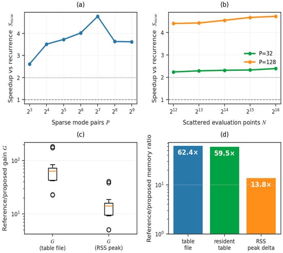
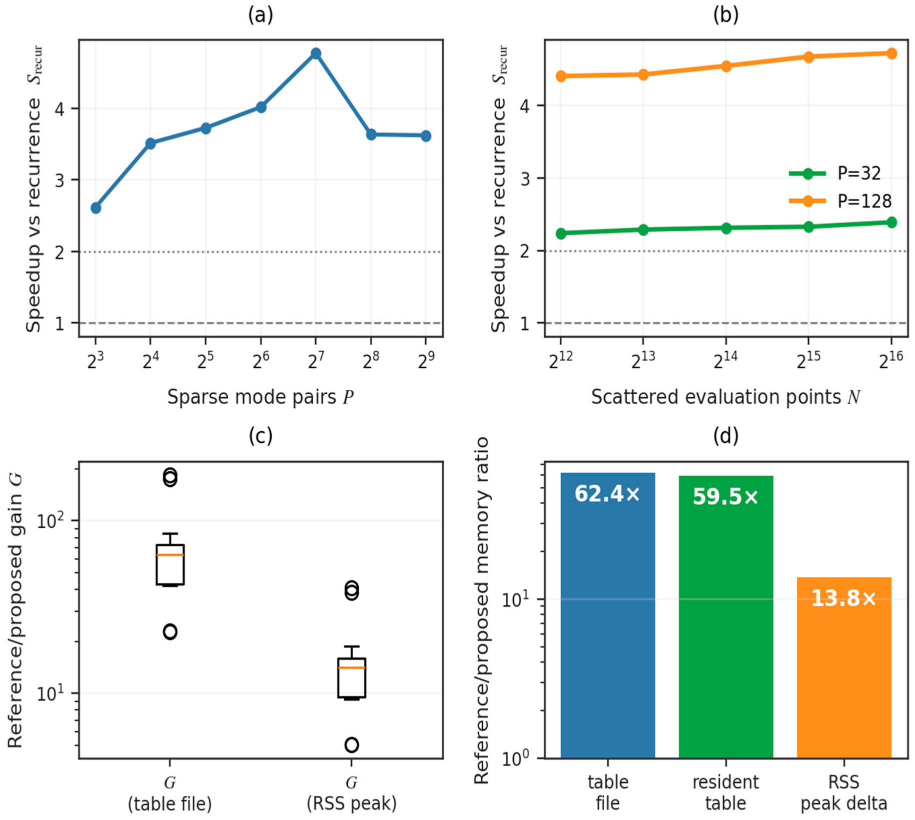
This subsection reports the $\theta$-dependent kernel evaluation of $K_{l,m}\left(\theta \right)$; common linear combinations and output formatting are excluded. Figure 3 summarizes the main performance results. Panels (c) and (d) quantify the memory advantage of the proposed method compared to the reference evaluator, whereas panels (a) and (b) quantify the speed advantage compared to the grouped recurrence baseline.

Figure 3. Performance and memory summary for mixed-mode/mixed-latitude workloads at L_max = 4096. (a) Recurrence-to-proposed speedup versus the number P of retained mode pairs at N = 32,768. (b) Speedup versus N for P = 32 and 128. (c) Reference-to-proposed time–memory improvement factor G across 25 cases. (d) Reference-to-proposed ratios for table file, resident table, and RSS peak delta; larger values favor the proposed method.

Figure 3c illustrates that the median time–memory improvement factor $G$ with respect to the reference evaluator lies within the resident-table-memory definition threshold by an approximate factor of 64, and within the RSS-peak-delta definition threshold by an approximate factor of 14. Figure 3d indicates that the reference-to-proposed memory ratios correspond to factors of approximately 62 for table file size, approximately 60 for resident table memory, and approximately 14 for RSS peak delta. Thus, the primary low-memory target is satisfied before comparing the speeds of the methods.

In the $P$ sweep, Figure 3a reveals speedup by a factor exceeding 2 across the entire sweep $P=8$–$256$ plus the auxiliary point $P=512$, with a maximum of 4.77 at $P=128$. In the $N$ sweep, Figure 3b reveals speedup by a factor of at least 2.25 for all representative cases with $N\ge 8192$, with 4.43–4.73 for $P=128$. These results indicate that for many scattered points and sparse mode sets, the batched surrogate evaluation outperforms grouped recurrence, despite the latter’s strong performance as a baseline. Under the strengthened measurement campaign (seeds 0, 1, 2 with 3 iterations), the seedwise medians of $S_{\mathrm{recur}}$ remain in the range 2.30–5.77 (median 4.39), corroborating the improvement by factors of “2–5 under representative conditions.”

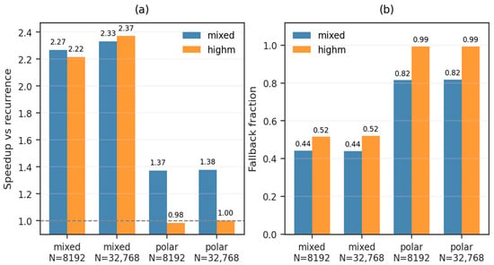
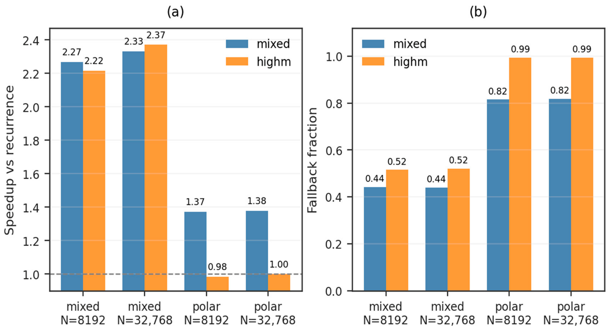
Under unfavorable conditions, particularly polar concentrations combined with high orders, the fraction of points eligible for surrogate evaluation is observed to decrease, with the hybrid evaluator approaching recurrence-level runtime. The most difficult case exhibits $S_{\mathrm{recur}}\approx 1$, indicating that the proposed method loses its speed advantage, but does not become substantially slower or unstable. The per-case values are listed in Supplementary Table S2.

Figure 4 describes the explicit relationship between speed ratio and fallback fraction. In mixed mode distributions, $S\approx 2.2$–$2.4$ and the fallback fraction remains at approximately 0.44–0.52. In contrast, under high-order polar conditions, $S\approx 0.98$–$1.00$ and the fallback fraction reaches 0.99. Thus, the surrogate-eligible fraction is a primary explanatory variable for the observed speed advantage. The internal runtime breakdown is provided in Supplementary Figure S3.

Figure 4. Effect of unfavorable mode and latitude distributions at L_max = 4096 and P = 32. Rows distinguish latitude distribution and point count N; colors distinguish mixed and high-order-concentrated mode sets. (a) Recurrence-to-proposed speedup, with parity marked at 1.0. (b) Fraction of mode–point evaluations routed to recurrence.

6.2. Memory Efficiency Comparison with Respect to the Reference Evaluator

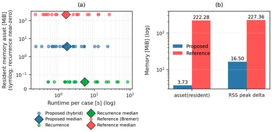
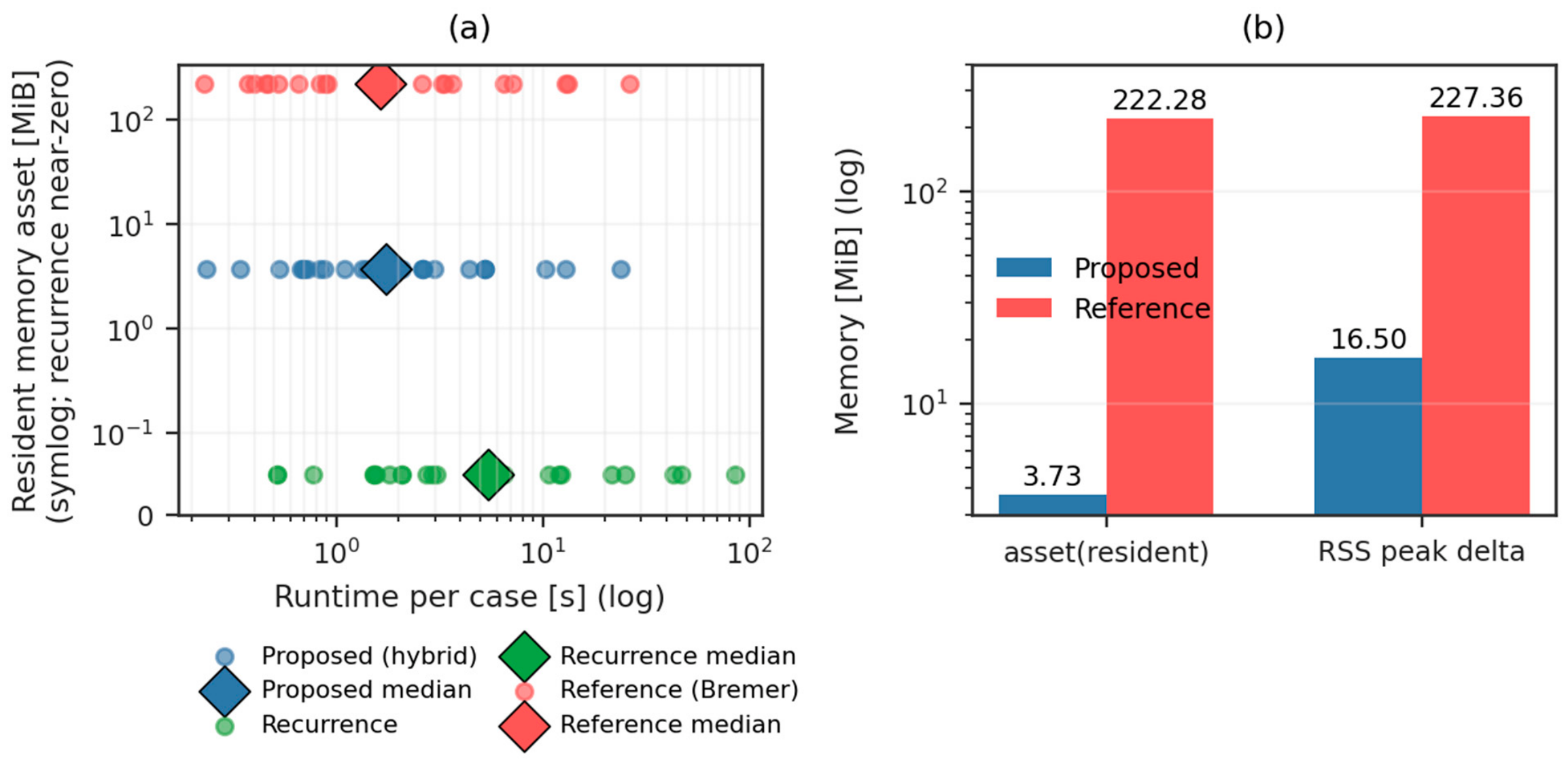
For 25 cases in total (8 unfavorable cases, 7 cases from the $P$ sweep, and 10 cases from the $N$ sweep), Figure 5a depicts the time–memory placement of the three methods and Figure 5b depicts their absolute memory comparison. The 222.28 MiB value for the reference evaluator corresponds to the resident memory of the default ALegendreEval binary table set (alegendre_data.bin1/2/3) as provided by the public implementation. Therefore, this is an implementation-level comparison and not a hypothetical minimum-size Bremer-type table optimized for our benchmark region.

Figure 5. Memory comparison under the C++-fair configuration. (a) Runtime versus resident evaluator-table memory across 25 cases; recurrence is near zero because it loads no evaluator table. (b) Resident-table memory and RSS peak delta for the proposed method and the public reference implementation.

Figure 5a indicates that the reference evaluator’s metric (red) crosses the 200 MiB threshold, the recurrence baseline (green) remains near zero because of its lack of a resident table, and the proposed method (blue) is concentrated at approximately 3–4 MiB. Figure 5b indicates the absolute values: the proposed table file size is 3.56 MiB and the resident table memory is 3.73 MiB, corresponding to reference/proposed ratios of 62.35 (file) and 59.55 (resident), respectively. Even for RSS peak delta, the proposed method uses 16.50 MiB of memory while the reference evaluator’s usage reaches 227.36 MiB, which represents a difference factor of approximately 14. The design goal—MiB-scale resident memory while maintaining ${10}^{-11}$-level agreement with the reference evaluator—is therefore achieved.

6.3. Agreement with the Reference Evaluator

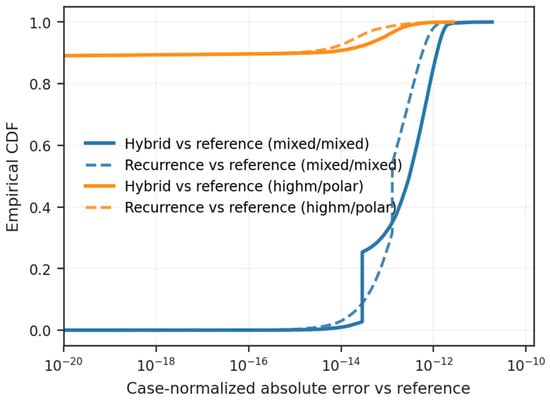
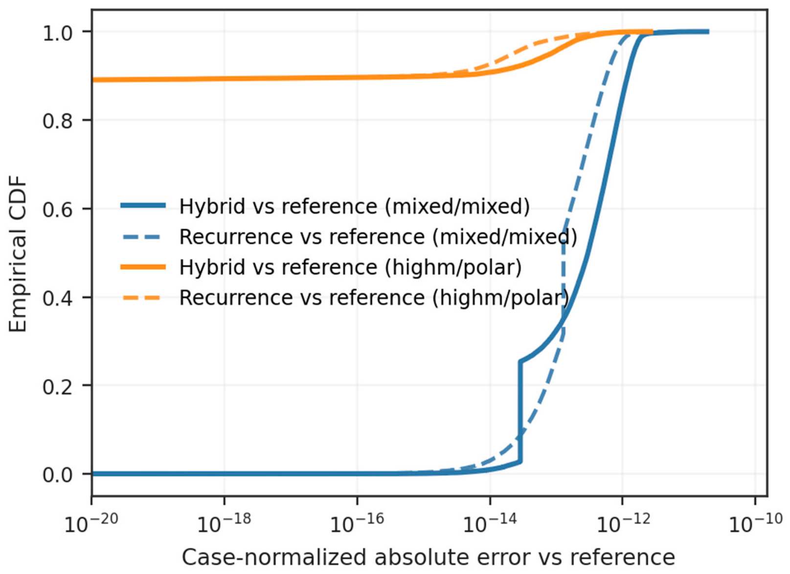
For the kernel-only cases considered in this subsection, the error metrics are computed over the stacked vector of evaluated kernel values $K_{l,m}\left({\theta }_i\right)$ for the sampled mode–point pairs. Across the 25 aforementioned cases combining the main sweeps and unfavorable conditions, the maximum relative difference remains below $4.1\times {10}^{-11}$. In the strengthened campaign (seeds 0, 1, 2; 3 iterations; $P=32$; $N=8192,\mathrm{32,768}$), it remains below $1.85\times {10}^{-11}$. Figure 6 illustrates the cumulative distributions for representative and unfavorable conditions. In both cases, the cumulative distribution functions of the proposed method (solid line) and recurrence (dashed line) almost overlap, indicating similar error characteristics. In the representative condition (mixed/mixed), the 99.9th percentile is given by $5.77\times {10}^{-12}$ and the maximum by $1.84\times {10}^{-11}$. In the unfavorable condition (highm/polar), the 99.9th percentile is $9.46\times {10}^{-13}$ and the maximum is $2.63\times {10}^{-12}$. These results indicate that guarded switching does not introduce visible error outliers within the tested domain. Supplementary Figure S4 reveals a different diagnostic conclusion, i.e., pointwise kernel relative errors along a single $\theta$ trace; its local peaks near zeros should not be compared directly with the case-normalized distributions in Figure 6. Supporting degree sweeps and ablations are illustrated in Supplementary Figures S1, S2 and S4.

Figure 6. Empirical cumulative distributions of case-normalized absolute errors for representative mixed/mixed and unfavorable highm/polar cases. Solid lines denote the proposed method and dashed lines the recurrence baseline; the metric is normalized by the maximum reference magnitude within each case, not by the pointwise value.

6.4. Scattered-Point Synthesis Including Longitude $\phi$ (End-to-End Validation)

The preceding results isolate the $\theta$-dependent kernel $K_{l,m}\left(\theta \right)$. However, actual applications require the full synthesis, including coefficients and longitudinal phase factors. Therefore, we evaluate whether the trends observed in the kernel benchmark persist in the end-to-end scattered-point synthesis. Under identical C++-fair configurations, we benchmark the synthesis, including terms of the form:

$$K_{l,m}\left({\theta }_i\right)\hspace{0.17em}\left(\mathrm{acos} \left(m{\phi }_i\right)+\mathrm{bsin} \left(m{\phi }_i\right)\right).$$

(42)

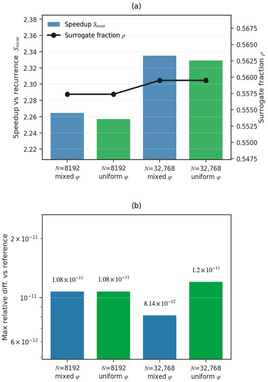
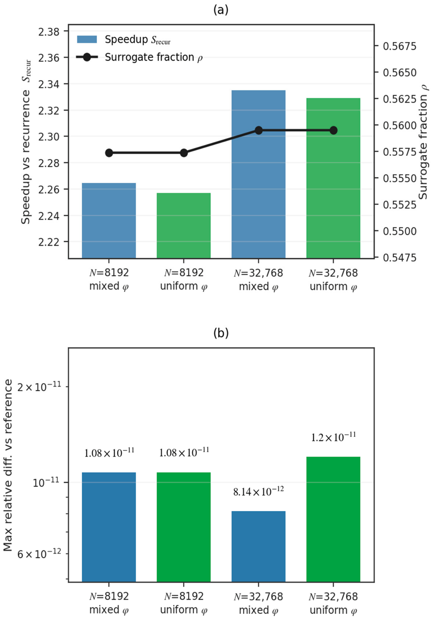
Figure 7 reveals four representative cases (two point counts and two longitude distributions) under the representative mixed/mixed condition. Figure 7a indicates that the speedup relative to recurrence remains in the range 2.26–2.34 in all four cases. The surrogate fraction $\rho$, plotted on the right axis, persist at approximately 0.56, indicating that changing the longitude distribution does not alter the main computational structure. Figure 7b indicates the maximum relative difference with respect to that of the reference evaluator. The maximum remains below $1.21\times {10}^{-11}$ in all cases, and the longitude distribution has minimal effect on the error level. Hence, the main claims are not limited to the simplified $\theta$-only benchmark; they also carry over to full scattered-point synthesis including longitudinal phase factors.

Figure 7. End-to-end scattered-point synthesis including longitude under the mixed/mixed condition at L_max = 4096. Four cases combine N = 8192 or 32,768 with uniform or clustered longitude distributions. (a) Speedup relative to recurrence and surrogate-handled fraction rho. (b) Maximum relative difference from the reference evaluator. In both panels, blue bars denote mixed-longitude cases and green bars denote uniform-longitude cases.

6.5. Auxiliary Metrics

The time–memory product is not the only possible metric. Therefore, we also aggregate throughput-per-memory and memory-budgeted maximum concurrent throughput across the 29 cases. These auxiliary metrics approximate the operational conditions of evaluation batches under a fixed memory budget. Therefore, they are useful for checking whether the memory advantage remains meaningful beyond the single-run measurements reported in Figure 3 and Figure 5. Under both the resident-table-memory and RSS-peak-delta definitions, the proposed method remains consistently favorable compared to the reference evaluator. Detailed min/median/max values are reported in Supplementary Table S3, and only the main representative ranges are listed in Table 2.

Table 2. Overall comparison of the methods. The Baseline column indicates whether each row is interpreted relative to recurrence or the reference evaluator. Here, indicates that the proposed method is faster than recurrence, and indicates that the proposed method is more favorable than the reference evaluator in terms of the memory-aware efficiency metric. Further, “table-free” indicates that the recurrence baseline has no resident evaluator table; it does not represent zero working memory. The 222.28 MiB value for the reference evaluator is the measured resident size of the public implementation as provided, not a benchmark region-optimized minimum configuration.

Comparison Framework	Baseline	Metric	Recurrence (Grouped by $\mathit{m}$)	Proposed	Reference Evaluator (ALegendreEval)
Speed	Recurrence	Throughput under representative distributions ($S_{\mathrm{recur}}$)	1×	2.25–4.77×	—
Speed	Recurrence	Throughput under unfavorable polar conditions ($S_{\mathrm{recur}}$)	1×	0.98–1.38×	—
Speed	Reference	Speed ratio against reference ($t_{\mathrm{ref}}/t$)	—	0.37–2.96	1×
Resident-table comparison	Reference	Table file size [MiB]	table-free	3.56	222.28
Resident-table comparison	Reference	Resident table memory [MiB]	table-free	3.73	222.28
Runtime measurement	Reference	RSS peak delta [MiB]	—	16.50	227.36
Accuracy	Reference	Maximum relative difference vs. reference	—	≤$4.1\times {10}^{-11}$	0 by definition
Efficiency metric	Reference	$G=F_{\mathrm{ref}}/F_{\mathrm{prop}}$ (resident-table-memory version)	—	22.86–184.75	—
Efficiency metric	Reference	$G=F_{\mathrm{ref}}/F_{\mathrm{prop}}$ (RSS-peak-delta version)	—	5.05–40.83	—

7. Discussion

7.1. Novelty and Design Principle

The novelty of this study transcends the mere combination of a known phase function method and known recurrence method—importantly, their roles are fixed in advance under an explicit resource constraint and the evaluator is closed under that constraint. The reference evaluator is used to create training samples offline; however, the runtime evaluator does not carry the reference table or call the reference implementation. Only the smooth generator functions $\varphi$ and $\psi$ are retained as Chebyshev coefficients. This converts the runtime problem from storing or querying a broad high-accuracy reference evaluator to evaluating a compact surrogate within a prescribed band-limit range.

The second design element is the guard. The surrogate is used only where the phase quantities are smooth and the finite-degree reconstruction is well conditioned. The physical evanescent region, the protected band on the oscillatory side of the turning point, m = 0 modes, and modes outside the fitted gamma range are routed to scaled recurrence. The proposed method is therefore not a pure approximation scheme: its approximation domain is explicitly bounded and the remaining domain is closed by a stable fallback path. This design explains why the difficult cases in Figure 4 retain acceptable accuracy even when the speed advantage is reduced.

Finally, the workload choice is also novel. This method is not intended to replace recurrence in full-grid transforms, where recurrence can reuse long contiguous degree ranges efficiently. Its advantage is manifested when the requested mode set is sparse, the point set is scattered, and the same sparse evaluation is required to be repeated several times. In this regime, the sequential degree traversal required by recurrence becomes undesirable, whereas the surrogate path reduces safe-region evaluation to the evaluation of independent fixed-degree polynomials.

7.2. Applicability and Limitations

The speed advantage of the proposed method lends it to a wide range of applications. In workloads where recurrence is naturally strong, particularly transforms that cover all modes and reuse contiguous $l$ ranges for the same $m$, the speed advantage is not guaranteed. The primary conclusions of this paper are centered on sparse mode sets, scattered points, and the many-point regime $N\ge 8192$. Under unfavorable conditions, such as polar concentrations with high-order concentrations, the surrogate region shrinks and the hybrid evaluator is reduced almost entirely to recurrence; with the speed advantage approaching recurrence-level runtime (Figure 4 and Supplementary Table S2). In such cases, the proposed method does not become unstable; rather, it behaves as designed by reverting to the safer recurrence path.

With respect to the reference evaluator, the central significance of the proposed method lies primarily in its large reduction in resident memory rather than in raw speed. The reported table-memory reduction by a factor of 60 can be interpreted as an implementation-level comparison against the public ALegendreEval table set used in this paper, but not as a lower bound on all possible Bremer-type implementations. Even with this qualification, the result is practically relevant because it reveals that a phase function-quality evaluator can be reorganized such that only an MiB-scale runtime table is required for the target band-limit range. Related works on non-equispaced spherical transforms and scattered-node approximation exist [24,25,26]. In addition, recent work has emphasized accelerated and differentiable spherical transforms, vector spherical harmonic transforms, and GPU-based non-uniform spherical harmonic transforms [27,28,29], while recent high-resolution geomagnetic model releases have expanded the application context for spherical-harmonic field evaluation [30]. These studies and products provide important background, but they address transform frameworks, vector transforms, full non-uniform transforms, or application-side field models; whereas, the current paper focuses on repeated associated-Legendre-kernel evaluations for sparse mode sets, as summarized in Supplementary Note S5. Additional scaling results on structured grids are provided in Supplementary Table S1.

Thus, this paper exhibits three explicit limitations. First, the proposed method does not claim to replace recurrence in dense full-band spherical harmonic transforms. Second, its speed advantage is conditional on a non-negligible surrogate-eligible fraction; when the workload lies almost entirely in guarded regions, the method intentionally behaves comparably to recurrence. Third, the comparison with ALegendreEval concerns the public implementation and table set used in this study; other implementations of Bremer-type phase methods may result in different memory–speed trade-offs.

The present validation is limited to L_max <= 4096. If L_max increases while P, N, and the Chebyshev degrees remain fixed, the point-dependent surrogate cost remains O(PN); whereas, the grouped-recurrence cost continues to depend on the accumulated degree-traversal lengths. The fallback fraction is governed primarily by the normalized ratio gamma and the latitude distribution rather than by L_max alone. Accuracy is less neutral: because a phase perturbation satisfies Delta alpha = lambda Delta phi, a fixed approximation error in phi is amplified as lambda grows. Maintaining the present tolerance beyond 4096 may therefore require higher polynomial degrees or subdivision of the parameter domain, with a corresponding increase in table memory. We consequently make no speed, accuracy, or memory guarantee beyond the validated bandlimit.

With respect to differentiation, spherical harmonic synthesis is linear in the spectral coefficients, so derivatives with respect to those coefficients are the evaluated basis values. Within either numerical path, derivatives with respect to theta can also be derived analytically. However, the current implementation uses a hard routing boundary and a pybind11 C++ kernel with no registered automatic-differentiation rule. The distributed implementation should therefore not be regarded as directly compatible with automatic-differentiation frameworks; such support would require a custom derivative rule and an explicit convention at routing boundaries.

7.3. Future Works

Future work should test the scaling expectations above for L_max > 4096, evaluate trajectory- or observation-derived point sets, extend the fused implementation to GPU-class architectures, and develop custom derivative rules where differentiable programming is required. These extensions would map the validity range of the method more completely without changing the claims established for the present CPU implementation and validated bandlimit.

8. Conclusions

In this paper, we present a guarded hybrid evaluator for associated Legendre functions in scattered-point sparse-mode workloads by combining a reference-based phase surrogate with scaled-recurrence fallback. The proposed method reduces the resident table memory by an approximate factor of 60 relative to the public reference implementation considered in this study, while maintaining agreement at the ${10}^{-11}$ level. Relative to recurrence, it achieves speedup by factors of 2–5 under representative conditions and falls back to recurrence-level runtime under the most difficult conditions. It outperforms the reference evaluator in terms of memory-aware efficiency metrics in all tested cases. The strengthened C++-fair comparison further corroborates that the advantage arises from structural differences in computation, rather than implementation-language artifacts. Sensitivity analyses and ablations are summarized in the Supplementary Information, and the reproducibility package is distributed alongside the manuscript. Future research should further clarify the validity range based on investigation of band-limit scaling, real-data point distributions, and GPU implementations. More broadly, the design principle developed in this paper, i.e., compressing smooth quantities that generate oscillatory functions and confining numerically delicate regions to stable fallback computation, may also serve as a guideline for the low-memory evaluation of other oscillatory special functions.

References

- IPCC. Climate Change 2021: The Physical Science Basis (Contribution of Working Group I to the Sixth Assessment Report of the IPCC); Cambridge University Press: Cambridge, UK, 2021. [Google Scholar] [CrossRef] [Scilit]
- World Meteorological Organization (WMO). State of the Global Climate 2023 (WMO-No. 1347); World Meteorological Organization (WMO): Geneva, Switzerland, 2024; Available online: https://wmo.int/publication-series/state-of-global-climate/state-of-global-climate-2023 (accessed on 3 March 2026).
- Evensen, G. Data Assimilation: The Ensemble Kalman Filter; Springer: Berlin/Heidelberg, Germany, 2009. [Google Scholar]
- Tarantola, A. Inverse Problem Theory and Methods for Model Parameter Estimation; SIAM: Bangkok, Thailand, 2005. [Google Scholar]
- Tapley, B.D.; Bettadpur, S.; Ries, J.C.; Thompson, P.F.; Watkins, M.M. GRACE Measurements of Mass Variability in the Earth System. Science 2004, 305, 503–505. [Google Scholar] [CrossRef] [Scilit] [PubMed]
- Drinkwater, M.; Floberghagen, R.; Haagmans, R.; Muzi, D.; Popescu, A. GOCE: ESA’s first Earth Explorer Core mission. Space Sci. Rev. 2003, 108, 419–432. [Google Scholar] [CrossRef] [Scilit]
- Friis-Christensen, E.; Lühr, H.; Hulot, G. Swarm: A constellation to study the Earth’s magnetic field. Earth. Planets Space 2006, 58, 351–358. [Google Scholar] [CrossRef] [Scilit]
- Driscoll, J.R.; Healy, D.M., Jr. Computing Fourier transforms and convolutions on the 2-sphere. Adv. Appl. Math. 1994, 15, 202–250. [Google Scholar] [CrossRef] [Scilit]
- Schaeffer, N. Efficient spherical harmonic transforms aimed at pseudospectral numerical simulations. Geochem. Geophys. Geosystems 2013, 14, 751–758. [Google Scholar] [CrossRef] [Scilit]
- Reinecke, M.; Seljebotn, D.S. Libsharp-spherical harmonic transforms revisited. Astron. Astrophys. 2013, 554, A112. [Google Scholar] [CrossRef] [Scilit]
- Górski, K.M.; Hivon, E.; Banday, A.J.; Wandelt, B.D.; Hansen, F.K.; Reinecke, M.; Bartelmann, M. HEALPix: A framework for high-resolution discretization and fast analysis of data distributed on the sphere. Astrophys. J. 2005, 622, 759–771. [Google Scholar] [CrossRef] [Scilit] [PubMed]
- Hale, N.; Townsend, A. A fast, FFT-based discrete Legendre transform. IMA J. Numer. Anal. 2016, 36, 1670–1684. [Google Scholar] [CrossRef] [Scilit]
- Holmes, S.A.; Featherstone, W.E. A unified approach to the Clenshaw summation and the recursive computation of very high degree and order normalised associated Legendre functions. J. Geod. 2002, 76, 279–299. [Google Scholar] [CrossRef] [Scilit]
- Ishioka, K. A new recurrence formula for efficient computation of spherical harmonic transform. J. Meteorol. Soc. Jpn. 2018, 96, 241–249. [Google Scholar] [CrossRef] [Scilit]
- Clenshaw, C.W. A note on the summation of Chebyshev series. Math. Comput. 1955, 9, 118–120. [Google Scholar] [CrossRef] [Scilit]
- Schaeffer, N. SHTns (software documentation, v3.7). Available online: https://gricad-gitlab.univ-grenoble-alpes.fr/schaeffn/shtns/-/tree/v3.7 (accessed on 3 March 2026).
- Bremer, J.; Rokhlin, V. On the nonoscillatory phase function for Legendre’s differential equation. J. Comput. Phys. 2017, 350, 326–342. [Google Scholar] [CrossRef] [Scilit]
- Bremer, J. An algorithm for the numerical evaluation of the associated Legendre functions that runs in time independent of degree and order. J. Comput. Phys. 2018, 360, 15–38. [Google Scholar] [CrossRef] [Scilit]
- Bremer, J. ALegendreEval (Software Repository, Commit e871d16). Available online: https://github.com/JamesCBremerJr/ALegendreEval/tree/e871d1649cfb11f5f26817e07ebefbb685ae0892 (accessed on 3 March 2026).
- NOAA NCEI Geomagnetic Modeling Team; British Geological Survey. World Magnetic Model 2025; NOAA National Centers for Environmental Information: Asheville, NC, USA, 2024. [CrossRef]
- NOAA National Centers for Environmental Information. Enhanced Magnetic Model (EMM). Available online: https://www.ncei.noaa.gov/products/enhanced-magnetic-model (accessed on 11 March 2026).
- Abramowitz, M.; Stegun, I.A. (Eds.) Handbook of Mathematical Functions with Formulas, Graphs, and Mathematical Tables; National Bureau of Standards Applied Mathematics Series 55; National Bureau of Standards: Gaithersburg, MD, USA, 1964. [Google Scholar]
- Trefethen, L.N. Approximation Theory and Approximation Practic; SIAM: Bangkok, Thailand, 2013. [Google Scholar]
- Kunis, S.; Potts, D. Fast spherical Fourier algorithms. J. Comput. Appl. Math. 2003, 161, 75–98. [Google Scholar] [CrossRef] [Scilit]
- Keiner, J.; Kunis, S.; Potts, D. Using NFFT 3—A software library for various nonequispaced fast Fourier transforms. ACM Trans. Math. Softw. 2009, 36, 19. [Google Scholar] [CrossRef] [Scilit]
- Filbir, F.; Themistoclakis, W. High-order scattered-data interpolation on the sphere and applications to the numerical solution of pseudo-differential equations. Math. Nachr. 2008, 281, 650–668. [Google Scholar] [CrossRef] [Scilit]
- Price, M.A.; McEwen, J.D. Differentiable and accelerated spherical harmonic and Wigner transforms. J. Comput. Phys. 2024, 510, 113109. [Google Scholar] [CrossRef] [Scilit]
- Le Gia, Q.T.; Li, M.; Wang, Y.G. Algorithm 1018: FaVeST—Fast Vector Spherical Harmonic Transforms. ACM Trans. Math. Softw. 2021, 47, 39. [Google Scholar] [CrossRef] [Scilit]
- Belkner, S.; Duivenvoorden, A.J.; Carron, J.; Schaeffer, N.; Reinecke, M. cunuSHT: GPU Accelerated Spherical Harmonic Transforms on Arbitrary Pixelizations. RAS Tech. Instrum. 2024, 3, 711–721. [Google Scholar] [CrossRef] [Scilit]
- NOAA NCEI Geomagnetic Modeling Team; British Geological Survey. World Magnetic Model High Resolution 2025; NOAA National Centers for Environmental Information: Asheville, NC, USA, 2024. [CrossRef]
Disclaimer/Publisher’s Note: The statements, opinions and data contained in all publications are solely those of the individual author(s) and contributor(s) and not of MDPI and/or the editor(s). MDPI and/or the editor(s) disclaim responsibility for any injury to people or property resulting from any ideas, methods, instructions or products referred to in the content. |
© 2026 by the authors. Licensee MDPI, Basel, Switzerland. This article is an open access article distributed under the terms and conditions of the Creative Commons Attribution (CC BY) license.