Operational Wheat-Yield Estimation in the Eastern Mediterranean Using Multi-Temporal Sentinel-2 Imagery and Explainable Machine Learning

Abstract

Accurate field-scale wheat yield estimation is essential for precision agriculture, farm-level decision-making, and food security planning. However, operational studies conducted under real commercial farming conditions in the eastern Mediterranean remain limited. This study investigated whether multi-temporal Sentinel-2 imagery could support reliable wheat yield estimation across nine commercial wheat fields near Ptolemaida, Greece, during the 2023–2024 growing season. Both durum and common wheat fields were included, and combine-harvester yield maps were used as ground-truth observations. Six regression algorithms—the Random Forest (RF), Support Vector Regression (SVR), k-nearest neighbors (KNN), Decision Tree (DT), LASSO regression, and Gaussian Process Regression (GPR) algorithms—were evaluated using three feature configurations: raw Sentinel-2 spectral bands only (Sentinel-only (SO)), spectral bands combined with vegetation indices (Sentinel+Indices, SI), and vegetation indices only (Indices-only, IO). Model generalization was assessed through a strict Leave-One-Field-Out (LOFO) cross-validation protocol, and the method of SHapley Additive exPlanations (SHAP) was used to interpret model behavior and identify the most influential spectral regions and phenological stages. RF achieved the highest predictive accuracy, with a MAPE of 7.90% and an RMSE of 45.15 kg decare⁻¹ under the SO configuration, demonstrating a statistically significant improvement over DT and KNN models ($p<0.05$). SHAP analysis indicated that model predictions were mainly driven by SWIR-1, NIR-narrow, and red-edge bands acquired during late grain filling and maturity, while vegetation indices contributed limited additional information. These findings suggest that raw multi-temporal Sentinel-2 spectral bands are highly effective for field-scale wheat yield estimation within the scope of this study, although further validation across diverse growing seasons and geographic regions is required to confirm broad operational sufficiency.

1. Introduction

Wheat (Triticum spp.) is a globally significant cereal crop and a key component of food security in Mediterranean and temperate agricultural regions [1]. Accurate and timely field-level crop-yield information is increasingly important for farmers, cooperatives, and policymakers because it supports decisions related to input management, risk assessment, and food-security planning [2]. Yield variability within and across fields is substantial and is influenced by complex interactions among soil properties, management practices, cultivar characteristics, and meteorological conditions [3]. Characterizing this spatial variability is essential for precision-agriculture interventions and for benchmarking field-scale performance against regional or national production targets [4,5].

1.1. Traditional vs. Remote Sensing Approaches

Traditional yield-estimation approaches typically include sparse field sampling, crop-cut surveys and process-based crop-growth modeling frameworks such as DSSAT (Decision Support System for Agrotechnology Transfer) and APSIM (Agricultural Production Systems Simulator). While these mechanistic models are physically interpretable and can simulate crop responses to environmental factors, they require detailed inputs such as soil hydraulic parameters, management calendars, and variety-specific coefficients. These inputs are often difficult to obtain at an operational scale, especially in commercial farming contexts [6,7,8]. Multiple studies have documented the substantial calibration and validation burdens associated with these models, including the need for site-specific soil data, weather inputs, and cultivar parameterization [9,10,11].

Satellite remote sensing [12] offers an alternative by providing spatially continuous and temporally dense observations that can track crop development throughout the growing season without the logistical constraints of in-field measurements [13,14]. Recent advances have demonstrated that integrating remote sensing data with machine learning approaches can achieve robust, scalable yield predictions while maintaining interpretability through hybrid frameworks combining mechanistic and data-driven methods [1,15].

1.2. Sentinel-2 Satellite Capabilities

The Sentinel-2 constellation, operated by the European Space Agency under the Copernicus program, provides high-spatial-resolution multispectral imagery at 10–20 m, with a five-day revisit time at the equator in the twin-satellite configuration [16]. Its red-edge, near-infrared (NIR) and shortwave infrared (SWIR) bands are particularly well suited for characterizing vegetation structure, chlorophyll content, leaf area index and canopy water status [4,17]. These spectral properties are closely linked to key physiological processes affecting grain yield, including canopy development, biomass accumulation, and senescence [13].

Multiple field-scale investigations in Mediterranean regions have demonstrated that Sentinel-2 red-edge bands can improve cereal-crop monitoring and yield estimation compared with conventional visible and NIR bands alone [17,18]. Studies using Sentinel-2 time series with machine-learning algorithms have reported high wheat-yield prediction accuracy across different Mediterranean environments, with reported $R^2$ values ranging approximately from 0.83 to 0.95 depending on crop type, study area, validation strategy, and modeling approach [4,5,13,19,20,21]. These studies employed diverse ground-truth validation approaches, including GPS-based combine-harvester yield maps [5], field-measured yields [13,21], and government-published statistics [4]. Together, they provide evidence that Sentinel-2 data can support field-scale wheat-yield modeling under operational farming conditions, while also highlighting the importance of validation design when comparing reported accuracy across studies.

Recent methodological developments have also examined the temporal aggregation of Sentinel-2 vegetation-index trajectories for wheat yield estimation. Ntouros et al. [22] applied an Area Under the Curve (AUC)-based approach to vegetation indices over predefined phenological windows in Western Macedonia, Greece, and reported that index trajectories during the period from tillering to grain filling were particularly informative for field-scale wheat yield estimation. In that study, GNDVI and LAI showed cultivar-specific relevance for durum and common wheat, respectively, with reported MAPE values of approximately 10–12%. Although this AUC-based approach is not directly compared with the machine learning feature configurations evaluated in the present study, it provides relevant regional and phenological context. In particular, it supports the importance of considering the timing of Sentinel-2 observations when extracting features for operational yield estimation.

1.3. Role of Machine Learning in Yield Estimation

Machine learning algorithms have become the dominant modeling framework for remote-sensing-based crop yield estimation owing to their ability to approximate complex, non-linear relationships between high-dimensional spectral features and agronomic outcomes without requiring explicit specification of underlying mechanisms [3,23]. Random Forest (RF) algorithms have consistently performed well across various crop types and geographic settings, demonstrating robustness to noise and the ability to capture non-linear interactions [4,13,20]. Support Vector Regression (SVR) and Gaussian Process Regression (GPR) have shown competitive or superior results in data-scarce scenarios and field-scale applications, with GPR being particularly effective in quantifying prediction uncertainty and generalizing across sampling scales [23,24].

Recent comparative studies have also highlighted the strong performance of gradient-boosted tree ensembles, such as Extreme Gradient Boosting (XGBoost) and CatBoost, which can match or exceed deep learning approaches while maintaining computational efficiency and interpretability [20,25]. Deep learning architectures, particularly Long Short-Term Memory (LSTM) networks and convolutional neural networks (CNNs), have demonstrated the capacity to leverage multisource time-series data combining remote sensing, meteorological, and soil inputs to explain substantial yield variance (∼71–86%) and capture temporal dependencies in crop development [1,3,21,26].

While ensemble methods and deep learning dominate recent literature, simpler approaches using linear regression on temporally integrated spectral features, such as AUC values of vegetation indices, have demonstrated competitive accuracy with significantly reduced computational complexity [22]. These findings suggest that, for operational applications where model transparency and computational efficiency are priorities, carefully engineered temporal features may offer an effective alternative to complex ensemble methods without a substantial decline in predictive performance.

1.4. Challenges and Advancements in Machine Learning

A persistent challenge in the remote sensing and machine learning literature for yield prediction is the risk of spatial overfitting. Many studies employ random cross-validation (CV), which can inflate reported accuracy by allowing spatially autocorrelated samples from the same field or neighboring fields to appear in both training and test sets, leading to overoptimistic performance estimates that do not reflect true generalization to unseen locations [27,28]. Evaluation protocols that explicitly account for spatial structure, such as spatial cross-validation or Leave-One-Field-Out (LOFO) cross-validation, offer a more realistic and conservative measure of model transferability to new parcels and are essential for assessing operational deployment readiness [28,29,30].

Multiple empirical studies have documented substantial drops in prediction accuracy on switching from random CV to spatial CV, confirming that spatial autocorrelation can systematically bias model evaluation. For example, Killeen et al. [27] demonstrated large reductions in correlation coefficients when spatial CV was applied to UAV-based corn yield prediction, and Radočaj et al. [28] found that spatial CV yields more conservative and realistic performance estimates than regular CV in Sentinel-2 maize yield experiments. Habibi et al. [29] compared random CV, spatial CV, and LOFO for soybean yield prediction, finding that spatial CV and LOFO provide more realistic transferability and that simpler models with feature selection improve extrapolation to new fields.

Despite their predictive power, machine learning models are often considered “black boxes”, hindering their adoption in operational agriculture where interpretability, mechanistic insight, and trust are crucial for end-user acceptance [31]. Recent advancements in explainable artificial intelligence (XAI), particularly SHapley Additive exPlanations (SHAP), address this limitation by providing theoretically grounded, model-agnostic, and consistent attributions of feature importance at both global and instance levels [32,33]. In remote sensing applications for agriculture, SHAP and related methods (e.g., integrated gradients) have been applied to identify the most predictive spectral bands, vegetation indices, and phenological stages for yield, offering mechanistic insight into model behavior and revealing key environmental drivers such as the enhanced vegetation index (EVI), vegetation optical depth (VOD), and temperature extremes [26,31,34]. SHAP-guided feature selection has also been shown to improve model accuracy and computational efficiency by removing negatively contributing features [35].

Beyond post hoc explainability methods, an alternative approach to fostering operational adoption focuses on developing accessible, user-friendly platforms that simplify the entire analytical workflow. Ntouros et al. [22] developed a web application implemented in Python (version 3.13.3) that integrates Google Earth Engine and automates Sentinel-2 data processing, from image acquisition through yield prediction, specifically targeting smallholder farmers and agronomists with limited geospatial expertise. By employing exclusively open-source software and eliminating barriers related to proprietary tools and complex preprocessing, such platforms can facilitate broader adoption of remote sensing technologies in precision agriculture, complementing efforts to make complex ML models more interpretable.

1.5. Current Study’s Focus

This study specifically addresses a gap in the existing literature by focusing on field-scale wheat crop-yield estimation under operational farming conditions in the eastern Mediterranean. It uses combine-harvester yield maps as ground truth, employs a rigorous LOFO evaluation strategy to ensure realistic assessment of spatial generalization, and applies SHAP-based interpretability analysis to multiple feature configurations derived from Sentinel-2 time series. The study area, near Ptolemaida in Western Macedonia, Greece, includes both durum wheat (Triticum durum) and common wheat (Triticum aestivum), allowing an assessment of model performance across two commercially relevant cultivar types within a single consistent analytical pipeline.

This regional focus is particularly relevant given recent validation studies in the same geographic area demonstrating cultivar-specific performance of vegetation indices, with GNDVI showing superior performance for durum wheat and LAI performing best for soft wheat [22]. The operational farming context and the use of combine-harvester yield maps align with best practices for field-scale remote sensing validation [4,5,13,20].

1.6. Specific Objectives

The specific objectives of this research are threefold:

1.

To evaluate the predictive performance of six regression algorithms (Random Forest, Support Vector Regression, k-nearest neighbors, Decision Tree, LASSO, and Gaussian Process Regression) using a strict LOFO cross-validation scheme that ensures spatial independence between training and testing data, following best practices for avoiding spatial overfitting [28,29].

2.

To compare three feature configurations derived from Sentinel-2 time series—raw spectral bands, spectral bands augmented with vegetation indices, and vegetation indices alone—in order to assess the relative value of spectral information at different levels of preprocessing and dimensionality. This comparison is informed by recent evidence that green- and red-edge-derived indices (GNDVI, LAI) provide superior predictive performance for wheat in Mediterranean conditions [17,22].

3.

To apply SHAP analysis to identify the spectral regions and phenological stages that most strongly drive model predictions, thereby providing interpretable insights into the remote sensing–yield relationship and revealing the biophysical mechanisms underlying successful yield estimation models. The analysis will specifically examine whether the critical phenological window from tillering to grain filling, identified by Ntouros et al. [22], emerges as the dominant temporal period in SHAP-based feature importance rankings.

By integrating robust spatial validation, comprehensive algorithm comparison, and explainable AI methods, this study contributes to the development of transparent, trustworthy, and operationally viable remote sensing tools for precision agriculture and food security decision-making. The findings will be contextualized within the broader landscape of operational tool development, including automated web-based platforms that facilitate technology transfer from research to practice.

2. Materials and Methods

2.1. Study Area

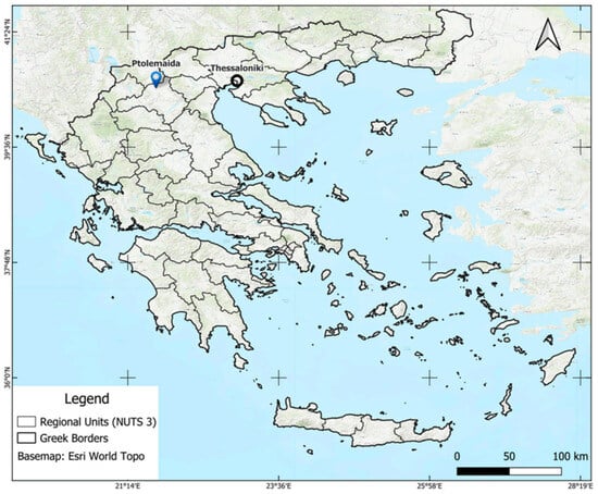
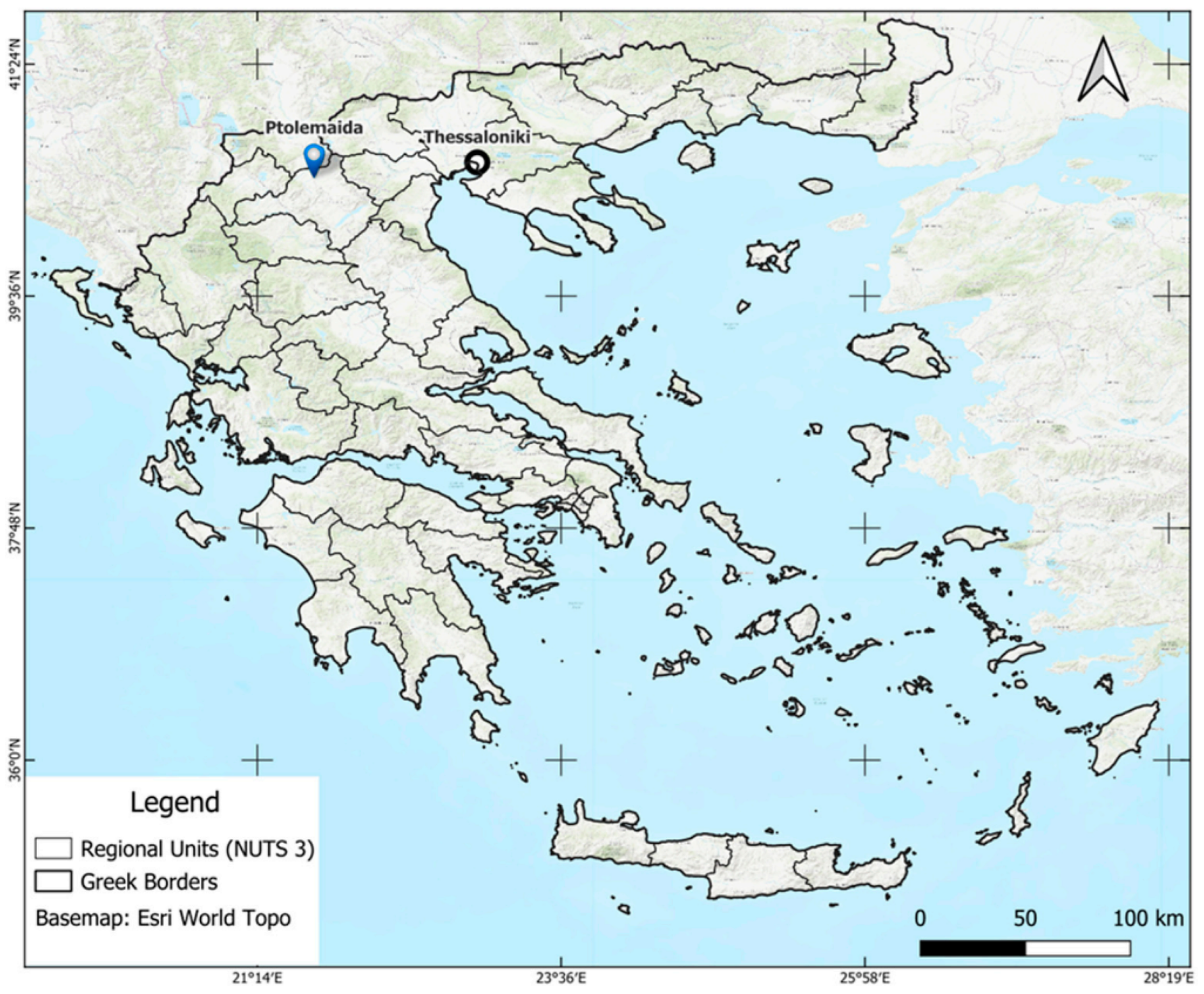
The study was conducted in nine operational commercial wheat fields located on the outskirts of Ptolemaida (latitude ≈ 40.51° N, longitude ≈ 21.68° E), in the Eordaia Municipality of Western Macedonia, northern Greece (Figure 1). The area lies at an elevation of approximately 600–650 m a.s.l. and is characterized by a semi-continental climate with cold, relatively wet winters and warm, dry summers. The production of cereal crops, particularly durum wheat, is the dominant agricultural activity in this part of Western Macedonia. The nine fields ranged in size from approximately 1 to 8 ha and were managed by a single farmer under standardized agronomic protocols, making them suitable for a controlled comparison of remote sensing modeling approaches.

Figure 1. Location of study fields in the Ptolemaida area, Western Macedonia, Greece (CRS: WGS84, EPSG: 4326).

2.2. Field Data: Yield Maps and Agronomic Management

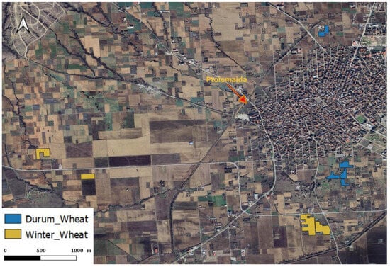
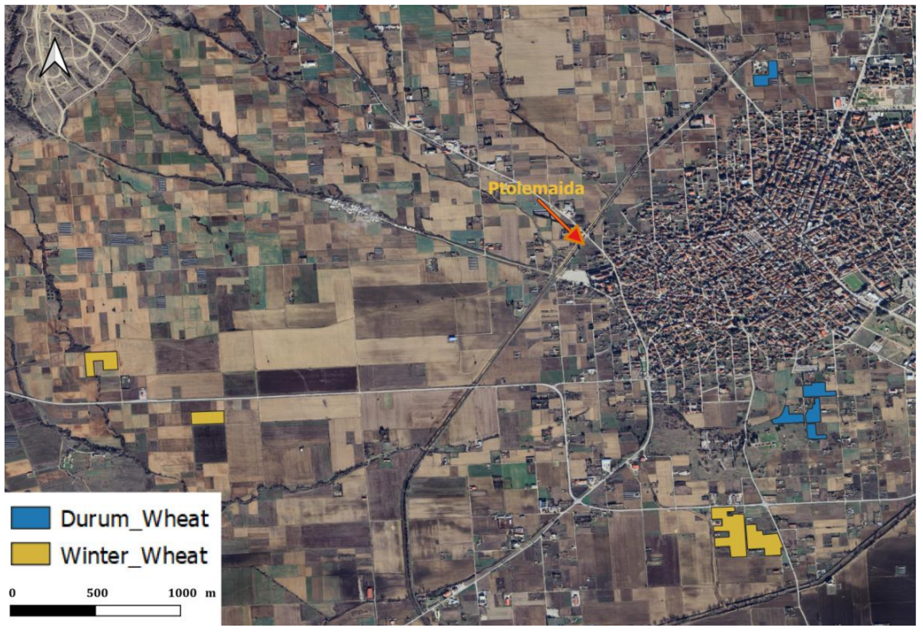
Five of the nine fields, located to the north and south of Ptolemaida, were cultivated with durum wheat (Triticum durum Desf., cultivar Svevo), while the remaining four, situated to the west and south of the town, were planted with common wheat (Triticum aestivum L., cultivar Giorgione), (Figure 2). Sowing across all fields was completed over the course of three to nine days.

Figure 2. Locations of the nine operational wheat fields under investigation, with the durum wheat (blue) and common wheat (yellow) parcels distinguished (CRS: WGS84, EPSG: 4326).

Because the study was conducted under commercial rather than controlled experimental conditions, sowing dates and agronomic management information were obtained through direct interviews with the farmer and cross-referenced, where possible, against publicly available meteorological and soil records. We acknowledge that interview-derived information may be subject to recall or reporting bias, particularly regarding the exact timing of field operations. However, these data were used only to describe the agronomic context of the study and were not included as direct predictive variables in the machine learning models.

Base fertilization was carried out in December with a compound fertilizer (N–P–K = 20–23–0) at a rate of 25 kg per decare (1000 m²); two supplementary nitrogen top-dressings (N–P–K = 40–0–0, 15 kg per decare each) were applied in early March and early April. Weed control was performed between 15 and 20 April using the herbicide Avoxa Maxx 12/2.88 OD (Syngenta, Basel, Switzerland), and fungal disease management was carried out in early May with Amistar Gold 12.5/12.5 SC (Syngenta). While management aimed for consistency, we acknowledge that inherent micro-variations in soil and field-level implementation may exist.

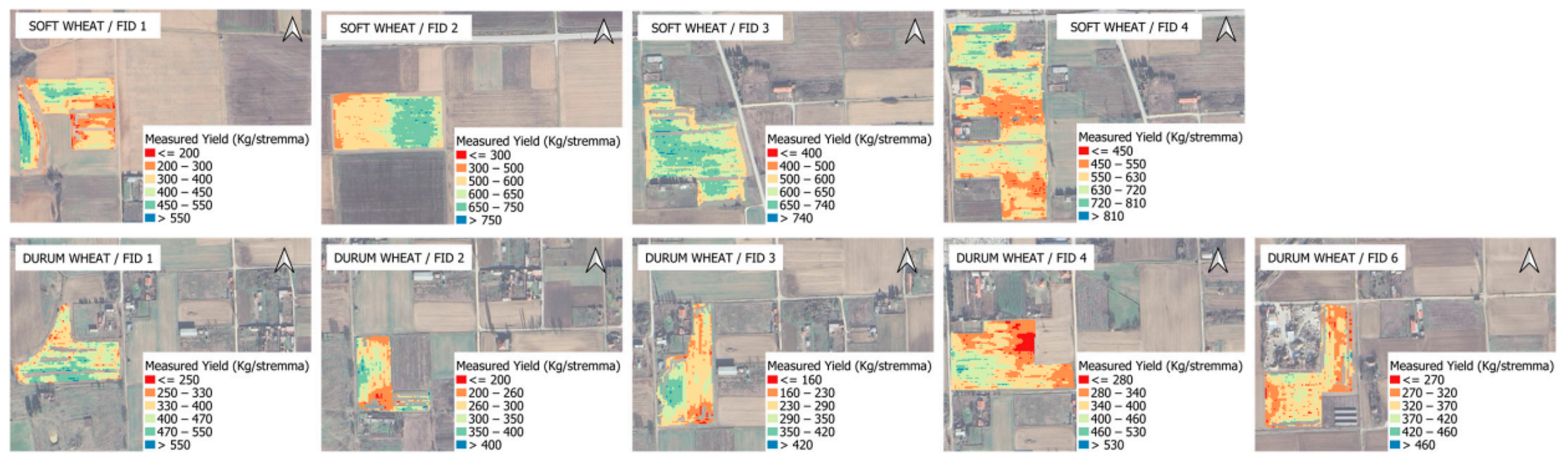
Actual yield data were collected using a FarmTRX^TM combine-mounted yield monitoring system (Troo Corporation, Ottawa, ON, Canada). The resulting point-cloud dataset was delivered in ESRI shapefile format and pre-processed to remove inaccurate records inherent to combine harvest dynamics (e.g., turnaround errors, header overlaps) and physically implausible yield values identified by an interquartile-range filter. Yield was expressed in kg per decare (1 decare = 1000 m²). Descriptive statistics for each field are reported in Table 1, and the spatial distribution of measured yield—interpolated to a regular grid using the Inverse Distance Weighting (IDW) method—is illustrated in Figure 3. The measured yield values showed a bimodal distribution, with common wheat fields achieving mean yields of 373–636 kg decare⁻¹ and durum wheat fields ranging from 259 to 426 kg decare⁻¹.

Table 1. Descriptive statistics of measured yield per operational field.

Crop	Field ID	Mean	Std. Dev.	Min	Max	Range
		(kg decare−1)
Common Wheat	FID 1	373.54	127.00	100.28	737.88	637.60
Common Wheat	FID 2	598.44	94.25	351.06	841.57	490.51
Common Wheat	FID 3	635.82	86.61	350.37	898.26	547.89
Common Wheat	FID 4	605.32	115.08	150.12	649.91	499.79
Durum Wheat	FID 1	425.59	105.98	150.12	649.91	499.79
Durum Wheat	FID 2	290.09	73.16	119.88	534.89	415.01
Durum Wheat	FID 3	258.73	82.42	61.04	542.13	481.09
Durum Wheat	FID 4	367.79	86.24	200.47	645.80	445.33
Durum Wheat	FID 6	339.34	63.99	200.60	561.36	360.76

1 decare = 1000 m².

Figure 3. Spatial distribution of measured yield per field: common wheat (top row) and durum wheat (bottom row), interpolated using IDW.

This pattern is reported here as a descriptive property of the ground-truth yield dataset. The objective of the present study was not to identify the agronomic or environmental causes of yield variability but to evaluate the ability of Sentinel-2-derived features and machine learning models to predict the measured yield values under operational farming conditions. Consequently, possible drivers of yield differences, including crop type, soil variability, microclimatic conditions, and management-related factors, were not analyzed separately as causal explanatory variables.

2.3. Meteorological and Soil Conditions

Meteorological data for the 2023–2024 growing season were obtained from the Ardassa automatic weather station (latitude 40.50° N, longitude 21.60° E, elevation 625 m), operated by the National Observatory of Athens; the data are publicly available via the METEO platform (https://www.meteo.gr/). The station is located approximately 5 km from the study fields. Monthly temperature and precipitation statistics for the growing season are summarized in Table 2. The season was characterized by cold, wet conditions in December and January (mean temperature $\approx 3.6$ °C, total precipitation 72.8 and 36.0 mm, respectively), followed by a gradual warming trend through spring. May and June were warm and dry (mean temperatures 16.4 and $24.4$ °C, precipitation 27.4 and 12.4 mm), conditions typical of the region during grain filling and harvest.

Table 2. Monthly climatic conditions over the 2023–2024 growing season (Ardassa weather station).

Month	Mean Temp. (°C)	Min Temp. (°C)	Max Temp. (°C)	Precipitation (mm)
December 2023	3.6	$-0.9$	11.7	72.8
January 2024	3.6	$-0.8$	8.8	36.0
February 2024	7.6	2.4	13.8	25.4
March 2024	9.3	3.5	15.8	45.2
April 2024	14.3	6.7	21.7	38.6
May 2024	16.4	10.9	22.4	27.4
June 2024	24.4	16.1	32.4	12.4

Soil characterization data were sourced from the publicly accessible Greek Soil Information System (https://www.opekepe.gr/opekepe-organisation-gr/opekepe-e-services-gr/pliroforiaka-systimata/gewpliroforiako-systima-edafologikwn-dedomenwn, accessed on 24 February 2025), as field-specific soil records were not available. The soil texture across common wheat fields ranged from moderately fine to fine, with luvisols and vertisols on alluvial terraces and deposits. The durum wheat fields were predominantly vertisols on alluvial deposits, with the exception of FID 6, which was a cambisol on alluvial terraces. While these data provide a reliable regional baseline, we acknowledge that sub-field soil heterogeneity may influence localized yield outcomes beyond the captured classes (Table 3).

Table 3. Soil characteristics of the examined wheat fields, derived from the Greek Soil Information System [36].

Crop Type	Field ID	Soil Type	Landscape/Parent Material	Drainage
Common wheat	FID 1-2	Luvisol	Alluvial terraces and deposits	Well drained
Common wheat	FID 3-4	Vertisol	Alluvial terraces and deposits	Well drained
Durum wheat	FID 1-4	Vertisol	Alluvial deposits	Well drained
Durum wheat	FID 6	Cambisol	Alluvial terraces; coarser texture	Well drained

2.4. Sentinel-2 Imagery

Sentinel-2 MSI Level 2A Surface Reflectance products were used throughout this study. Level-2A data are atmospherically corrected bottom-of-atmosphere (BOA) reflectance values generated by the Sen2Cor processor and distributed freely through the Copernicus Data Space Ecosystem. Ten spectral bands were retained for analysis (Table 4), covering the blue, green, red, three red-edge, NIR, NIR-narrow and two SWIR regions. All 20 m bands were resampled to 10 m using bilinear interpolation to establish a common spatial reference grid.

Table 4. Sentinel-2 MSI bands retained for analysis.

Band	Spectral Region	Central Wavelength (nm)	Native Resolution (m)
B2	Blue	490	10
B3	Green	560	10
B4	Red	665	10
B5	Red-edge 1	705	20
B6	Red-edge 2	740	20
B7	Red-edge 3	783	20
B8	NIR	842	10
B8A	NIR-narrow	865	20
B11	SWIR 1	1610	20
B12	SWIR 2	2190	20

A total of 14 acquisition dates were used, spanning the 2023–2024 growing season from emergence to post-harvest (Table 5). Images were selected to provide coverage at each key phenological stage as defined by the BBCH scale, prioritizing nearly cloud-free acquisitions.

Table 5. Sentinel-2 acquisition dates and corresponding BBCH phenological stages.

Phenological Stage	Duration	BBCH Scale	Acquisition Date(s)
Emergence	7–14 days	BBCH 10–19	13 January 2024
Tillering	25–40 days	BBCH 20–29	26 January; 15 February; 17 February; 22 February 2024
Stem Elongation	20–30 days	BBCH 30–39	3 March; 21 March 2024
Booting	20–30 days	BBCH 40–49	28 March 2024
Heading	7–14 days	BBCH 51–59	15 April 2024
Flowering	5–10 days	BBCH 61–69	7 May 2024
Grain Filling	10–20 days	BBCH 71–77	22 May; 27 May 2024
Maturity/Harvest	10–20 days	BBCH 83–99	9 June 2024
Post-harvest	-	-	24 June 2024

2.5. Vegetation Indices

In addition to the raw spectral bands, a set of vegetation indices was computed for each acquisition date to capture complementary aspects of canopy biophysics relevant to wheat yield, including canopy greenness, chlorophyll content and water status [37]. The Normalized Difference Vegetation Index (NDVI) and the Green NDVI (GNDVI) describe general canopy vigor; the Normalized Difference Moisture Index (NDMI) and the SWIR-based moisture stress index (NDMSI) capture canopy water content; and the red-edge chlorophyll index (CIre) and the MERIS Terrestrial Chlorophyll Index (MTCI) are sensitive to chlorophyll concentration and nitrogen status.

2.6. Feature Configurations and Data Integration

Three feature configurations were constructed: Sentinel-only (SO), Sentinel+Indices (SI), and Indices-only (IO). Sentinel-2 stacks, derived indices, yield maps, and parcel boundaries were co-registered onto a 10 m reference grid. All input features were normalized using min–max scaling to the range $[0,1]$ prior to model training. Target yield values were also scaled during training to ensure numerical stability and consistent gradient behavior for models such as SVR and LASSO. Inverse scaling was applied to all outputs to obtain predictions in kg decare⁻¹ for evaluation.

2.7. Machine Learning Models

Six regression algorithms were evaluated: Random Forest (RF), Support Vector Regression (SVR), k-nearest neighbors (KNN), Decision Tree (DT), LASSO regression, and Gaussian Process Regression (GPR). RF is consistently strong in remote-sensing-based crop studies. GPR is a Bayesian non-parametric approach providing predictive uncertainty alongside point predictions [38].

2.8. Model Evaluation: Leave-One-Field-Out Cross-Validation

Model generalization was assessed using a strict Leave-One-Field-Out (LOFO) cross-validation scheme. This protocol prevents spatial leakage and provides a realistic estimate of out-of-parcel prediction accuracy. Within each fold, hyperparameters were optimized using RandomizedSearchCV applied exclusively to training data (inner three-fold cross-validation, $n_{\mathrm{iter}}\le 8$ iterations). The search budget of 8 iterations was selected to balance computational efficiency across the multiple LOFO folds while focusing on literature-informed parameter ranges.

2.9. Final Model Selection and SHAP Interpretability

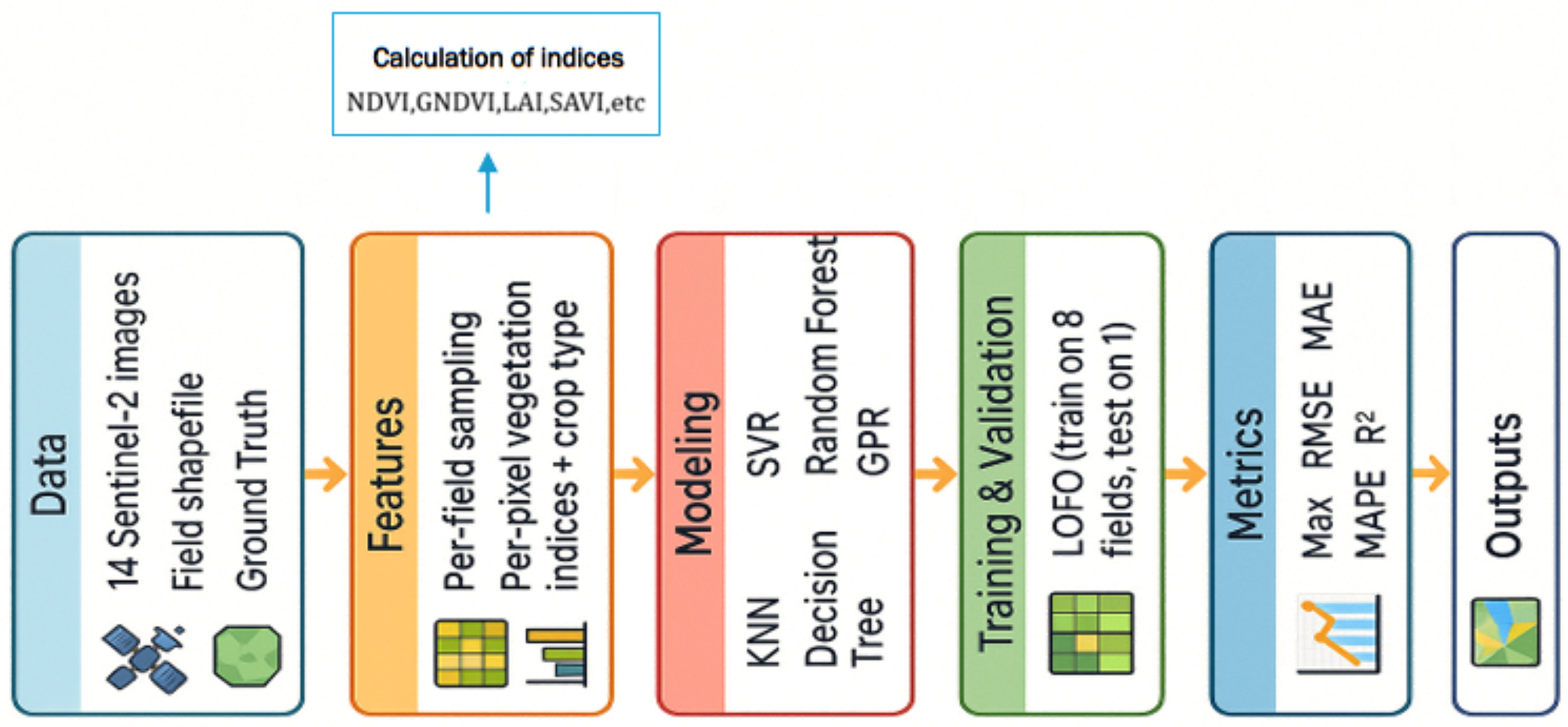
The algorithm achieving the highest mean test $R^2$ was selected. The final operational model was retrained on all available pixels to leverage the full seasonal information, while the LOFO metrics provided the unbiased estimates of generalization [39]. Model behavior was interpreted using SHapley Additive exPlanations (SHAP). Global importance was visualized via SHAP beeswarm plots. A schematic overview of the complete processing pipeline is provided in Figure 4.

Figure 4. Complete processing pipeline, from Sentinel-2 data ingestion through LOFO cross-validation to SHAP interpretability analysis.

3. Results

3.1. Model Performance

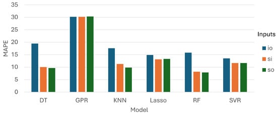
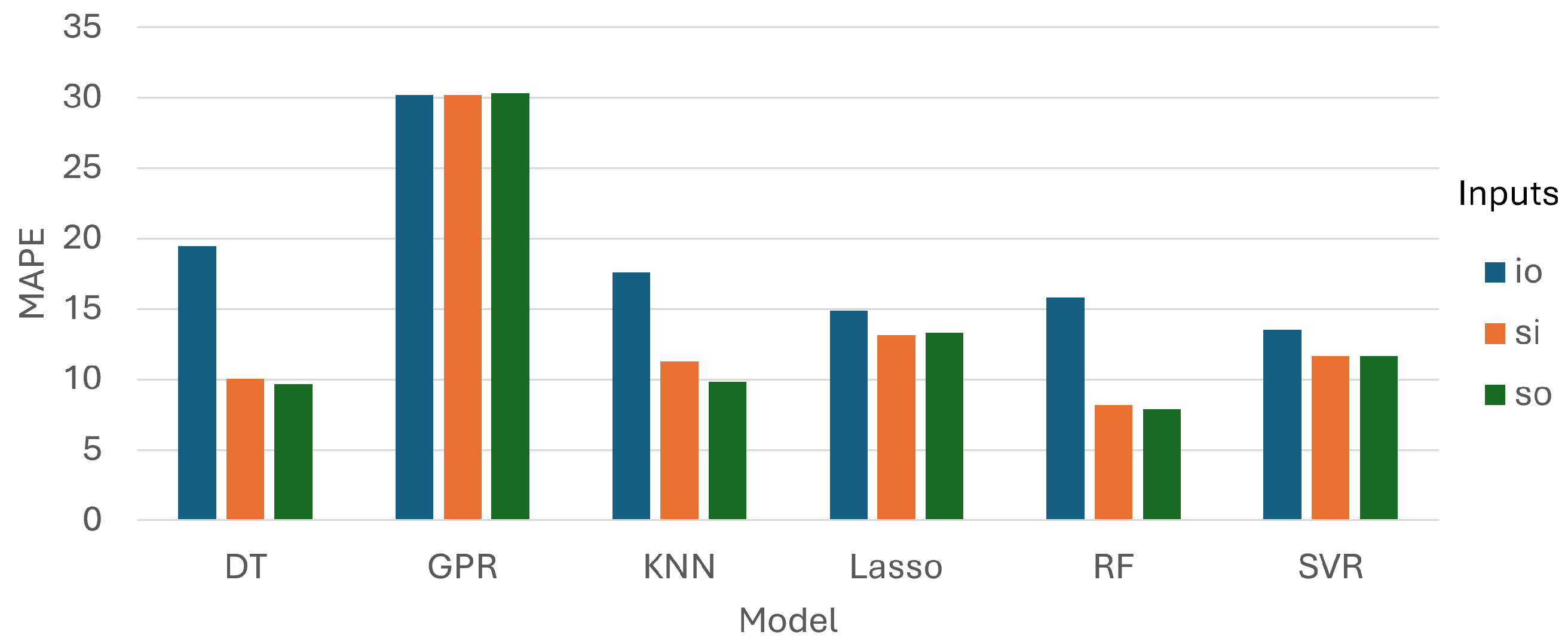
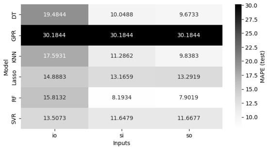
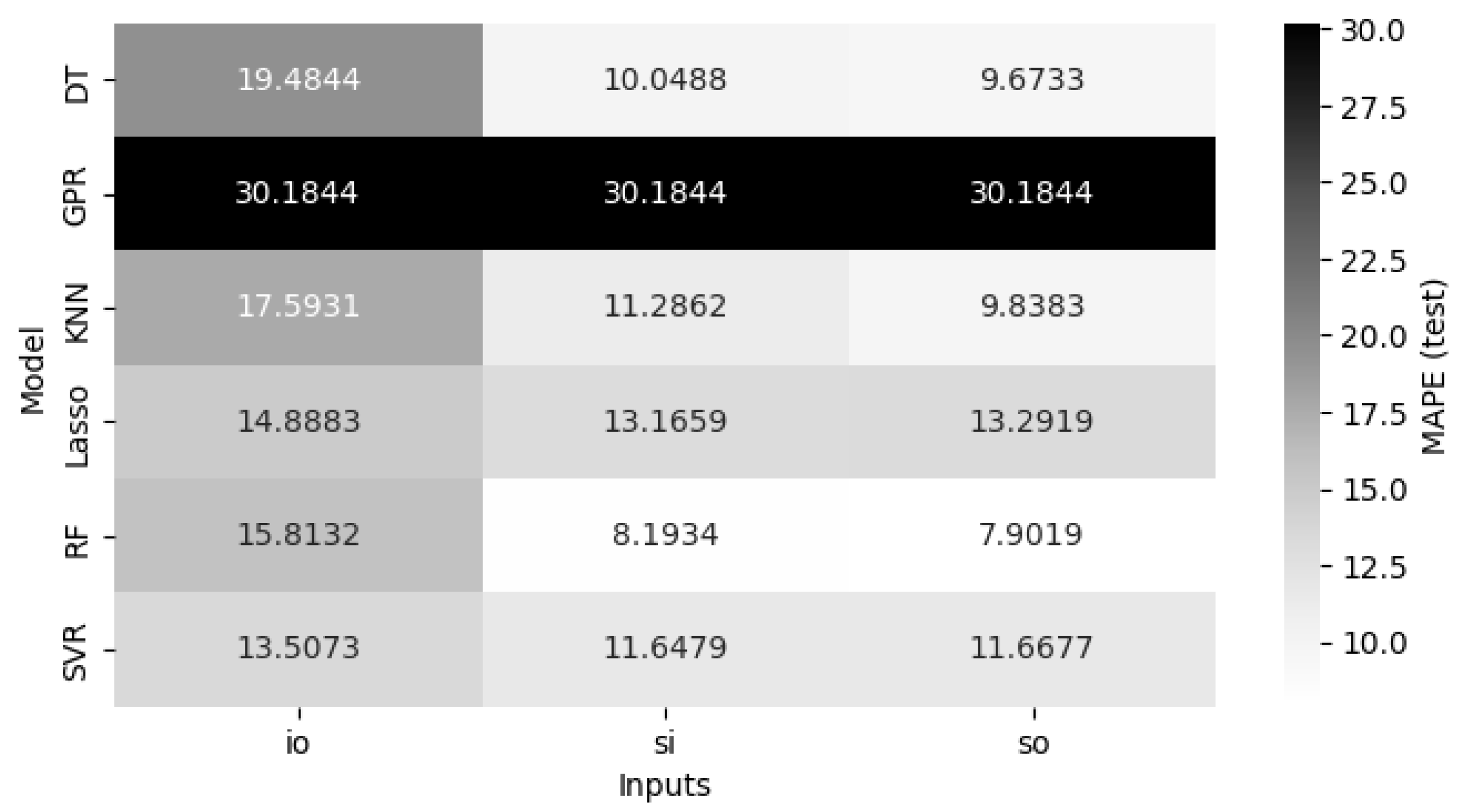
The MAPE scores across all models and feature configurations for the test set are presented in Figure 5. Random Forest achieved the lowest test MAPE under both Sentinel-based configurations, recording 7.90% on Sentinel-only (SO) and 8.19% on Sentinel and Indices (SI). This difference of less than 0.3 percentage points was within the cross-fold variability of the experiment. KNN and DT followed a consistent pattern, with SO yielding MAPE values of 9.84% and 9.67%, respectively, and both models showing a substantial degradation when restricted to the Indices-only (IO) configuration (17.59% and 19.48%). SVR and LASSO performed more uniformly across SI and SO, with MAPE values in the range of 11.65–13.29%, while IO induced a moderate but consistent increase in error for both.

Figure 5. MAPE values for the test sets.

The GPR exhibited weaker out-of-field generalization under the LOFO protocol. Accordingly, the performance was further assessed in terms of MAPE values among training data. The provided values were compared against the RF regressors (in parentheses). The average values were as follows: (a) IO scenario: 0.88% (6.52%); (b) SO scenario: 0.88% (3.72%); and (c) SI scenario: 0.88% (3.81%). No kernel diagnostics or covariance analyses were conducted, and therefore no definitive explanation is provided, since this is outside the scope of the present study.

The heatmap in Figure 6 further illustrates that the SO and SI columns were nearly indistinguishable in magnitude across all competitive models, whereas the IO column was systematically elevated. This pattern indicates that raw spectral bands provided the dominant predictive signal, while derived vegetation indices added limited incremental information in this dataset. GPR exhibited consistently elevated MAPE values (≈30.2%) regardless of the feature configuration, indicating weak out-of-field generalization under the LOFO protocol. Because no additional kernel-conditioning or covariance-diagnostic analysis was performed, no specific mechanistic cause for the poor GPR performance is inferred here.

Figure 6. Heatmap of the MAPE values for the test sets.

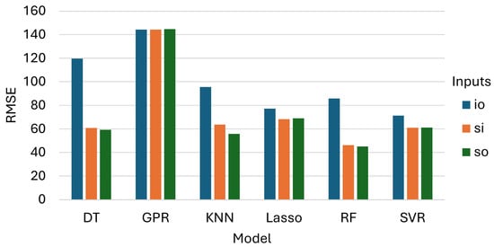
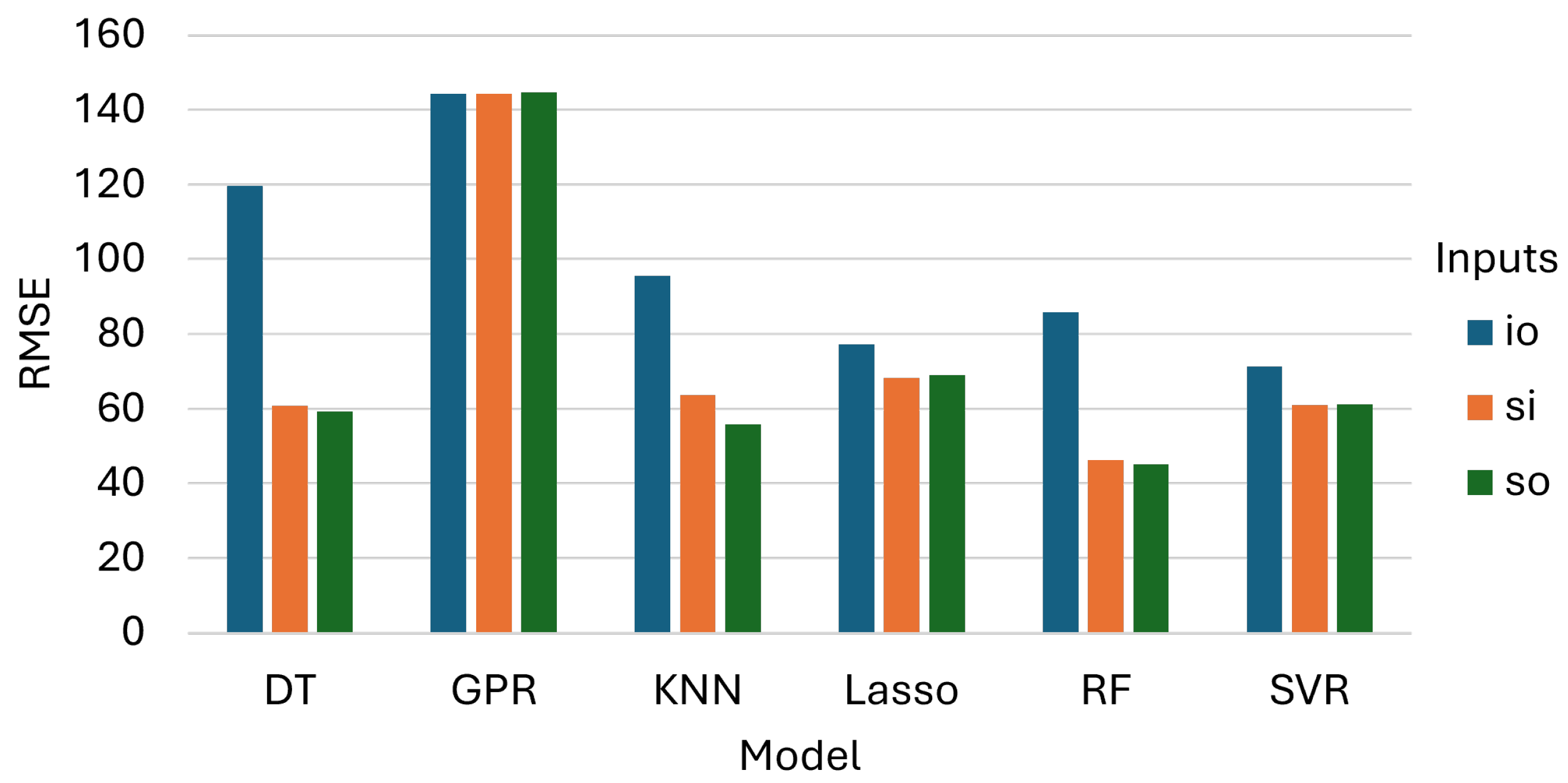
The test-set RMSE values, reported in Figure 7, were consistent with the MAPE findings and reinforced the same model and configuration ranking. RF achieved the lowest RMSE under SO ($45.15$ kg decare⁻¹) and SI ($46.33$ kg decare⁻¹), with a marginal difference of approximately $1.2$ kg decare⁻¹ between the two configurations. KNN and DT recorded RMSE values of $55.78$ and $59.34$ kg decare⁻¹ under SO, respectively, and both showed marked increases when evaluated on IO alone ($95.65$ and $119.64$ kg decare⁻¹). SVR and LASSO presented moderate and relatively stable RMSE values across SI and SO (≈61–69 kg decare⁻¹), with IO inducing a deterioration that was noticeable but less severe than with the non-linear learners. GPR yielded the highest RMSE across all configurations (≈144.4–144.6 kg decare⁻¹) and, unlike the other models, showed little sensitivity to the choice of feature set. This result further indicates that GPR did not effectively exploit the available spectral information in the out-of-field generalization setting.

Figure 7. RMSE values for the test sets.

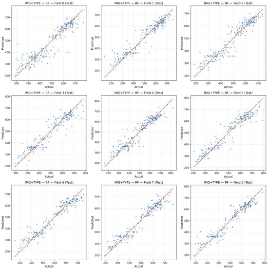
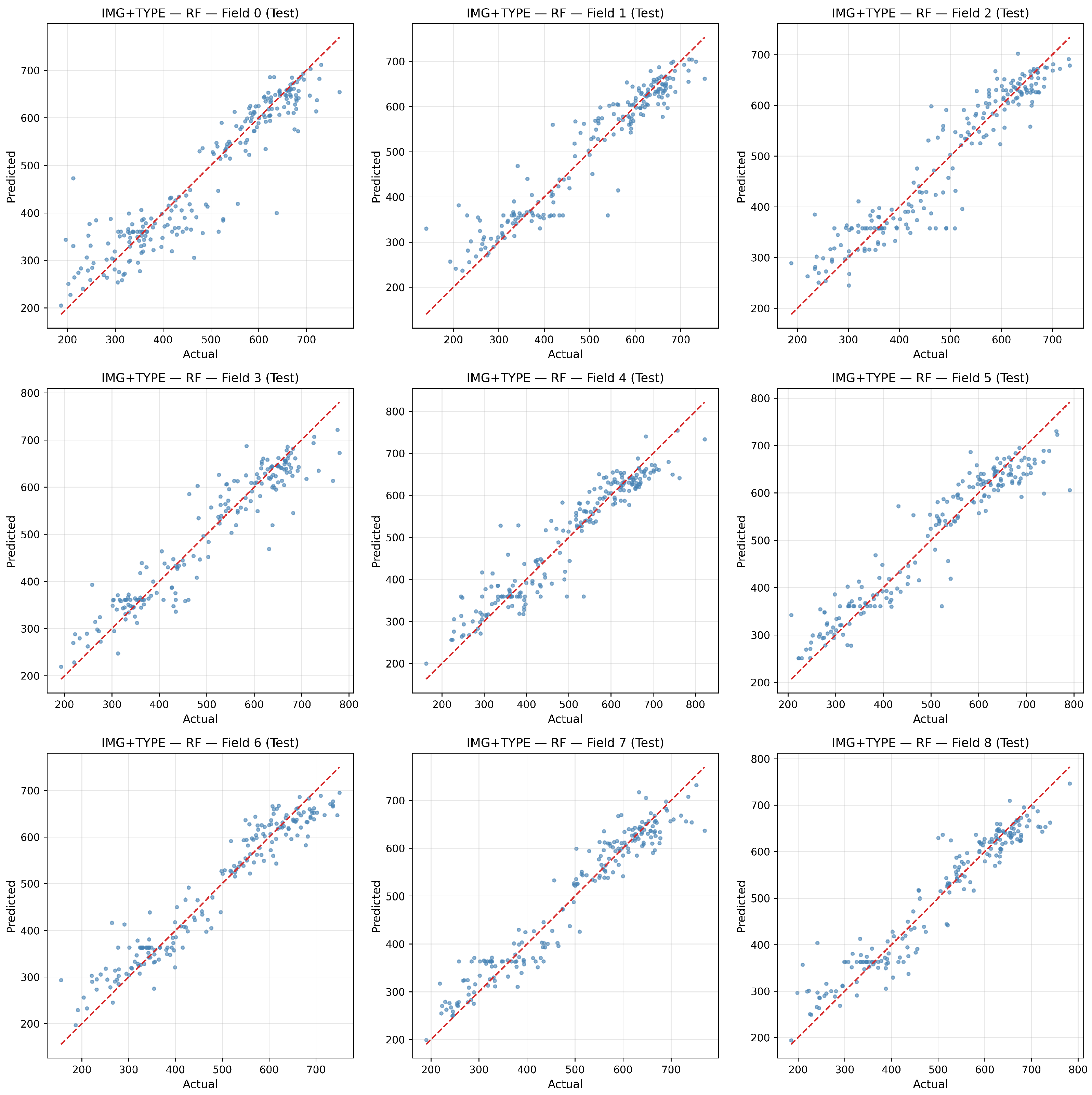
Under the Sentinel-only configuration (Figure 8), several fields exhibited equal or slightly tighter clustering around the 1:1 line, particularly mid-range. This pattern mirrors the small but consistent $R^2$ advantage observed for RF when using spectral bands alone. These results suggest that, once the raw Sentinel-2 spectral bands are available, vegetation indices contribute limited additional predictive information to this dataset. Residual spread was concentrated at the distribution extremes, which is a common pattern for agronomic endpoints.

Figure 8. Predicted vs. actual yield per field in the test set for RF using Sentinel-only inputs.

3.2. Statistical Analysis

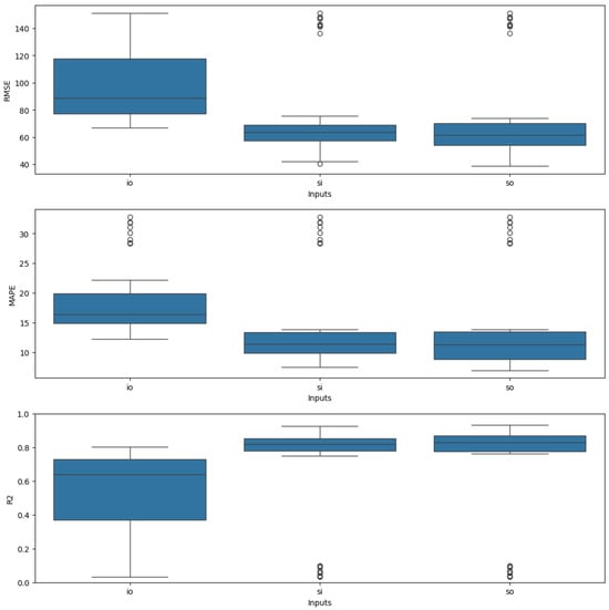
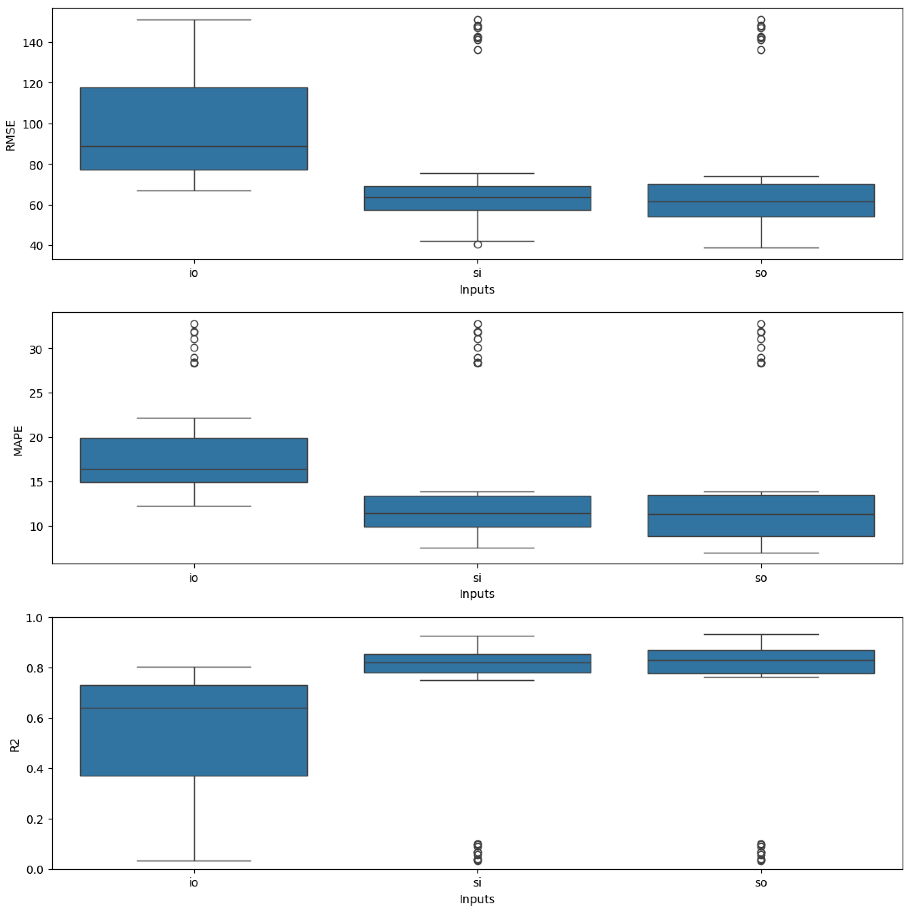
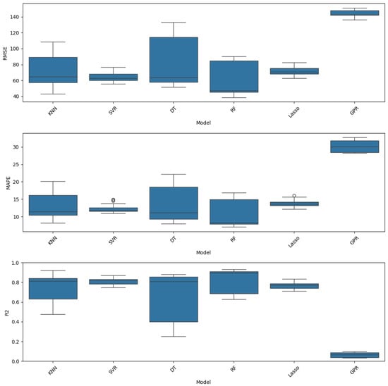
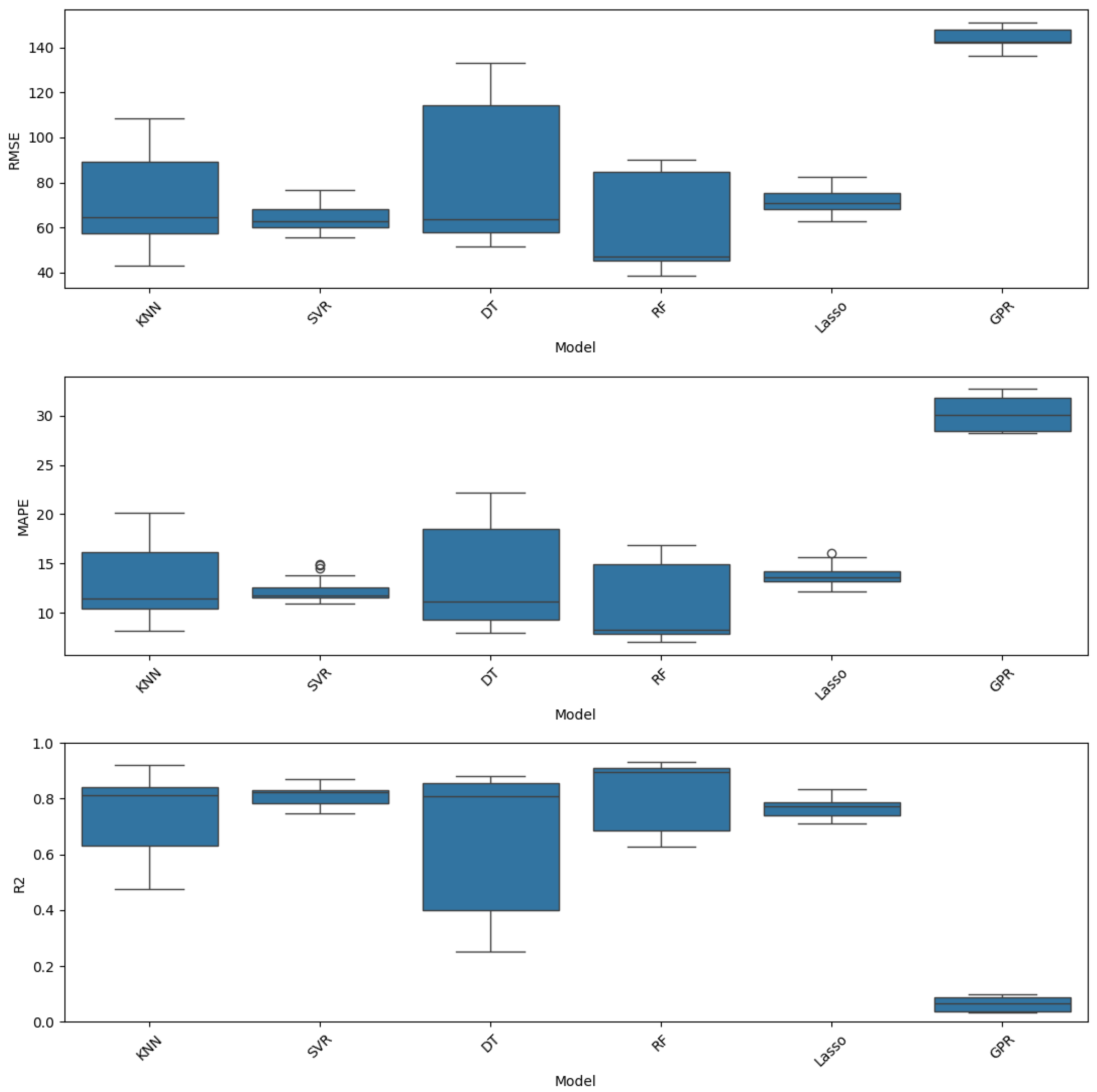
The box plots presented in Figure 9 and Figure 10 reveal broadly overlapping performance distributions across both models and feature configurations, particularly between the SI and SO input sets, which motivates a formal statistical comparison rather than reliance on point estimates alone. To assess whether the observed differences in $R^2$, RMSE, and MAPE are statistically significant, a series of hypothesis tests were conducted.

Figure 9. Performance scores by input type.

Figure 10. Performance scores by regression model.

Prior to any inferential analysis, the assumptions underlying a parametric one-way ANOVA were examined. The Shapiro–Wilk test for residual normality yielded a statistic of $W=0.982$ with $p=0.033$, and Levene’s test for homogeneity of variance across groups produced a statistic of $3.776$ with $p<0.001$. As both assumptions were violated, a non-parametric framework was adopted for all subsequent comparisons.

The Kruskal–Wallis test was applied separately to the model factor and the input configuration factor. With respect to the model factor, a highly significant result was obtained ($H=80.25$, $p<0.001$), indicating that the performance distributions were not equivalent across all six algorithms. Pairwise Mann–Whitney U tests with the Holm–Bonferroni correction were subsequently conducted to identify the source of these differences. GPR was found to differ significantly from every other model (all corrected $p_{\mathrm{Holm}}<0.001$), consistent with its substantially elevated error levels discussed in the preceding section. Among the remaining five models, SVR was found to differ significantly from LASSO ($p_{\mathrm{Holm}}<0.001$), and RF differed significantly from both DT ($p_{\mathrm{Holm}}=0.020$) and KNN ($p_{\mathrm{Holm}}=0.022$). All other pairwise comparisons among the non-GPR models—including RF vs. LASSO, SVR vs. RF, KNN vs. SVR, and KNN vs. DT—did not reach statistical significance after correction ($p_{\mathrm{Holm}}>0.05$), indicating that their performance distributions are statistically indistinguishable. Table 6 provides the detailed results for the pairwise comparisons regarding the model’s performance.

Table 6. Pairwise comparisons after Kruskal–Wallis test for model performance. Kruskal–Wallis statistic: $H=80.2517$, $p<0.001$. Holm–Bonferroni correction applied.

Group 1	Group 2	U Statistic	praw	pHolm
KNN	GPR	0	$2.95\times {10}^{-10}$	$4.42\times {10}^{-9}$
LASSO	GPR	0	$2.95\times {10}^{-10}$	$4.13\times {10}^{-9}$
DT	GPR	0	$2.95\times {10}^{-10}$	$3.83\times {10}^{-9}$
SVR	GPR	0	$2.95\times {10}^{-10}$	$3.54\times {10}^{-9}$
RF	GPR	0	$2.95\times {10}^{-10}$	$3.24\times {10}^{-9}$
SVR	LASSO	114	$1.53\times {10}^{-5}$	$1.53\times {10}^{-4}$
DT	RF	542	$2.20\times {10}^{-3}$	$1.98\times {10}^{-2}$
KNN	RF	538	$2.76\times {10}^{-3}$	$2.21\times {10}^{-2}$
RF	LASSO	224	$1.54\times {10}^{-2}$	$1.08\times {10}^{-1}$
SVR	RF	491	$2.93\times {10}^{-2}$	$1.76\times {10}^{-1}$
DT	LASSO	243	$3.63\times {10}^{-2}$	$1.82\times {10}^{-1}$
KNN	LASSO	251	$5.06\times {10}^{-2}$	$2.02\times {10}^{-1}$
SVR	DT	474	$5.93\times {10}^{-2}$	$1.78\times {10}^{-1}$
KNN	SVR	309	$3.41\times {10}^{-1}$	$6.83\times {10}^{-1}$
KNN	DT	387	$7.04\times {10}^{-1}$	$7.04\times {10}^{-1}$

Regarding the input configuration factor, the Kruskal–Wallis test once again yielded a significant result ($H=47.79$, $p<0.001$). Pairwise comparisons revealed that IO differed significantly from both SI ($p_{\mathrm{holm}}<0.001$) and SO ($p_{\mathrm{holm}}<0.001$), confirming that the exclusion of raw spectral bands leads to a statistically meaningful degradation in predictive performance. Critically, no significant difference was detected between SI and SO ($U=1562.5$, $p_{\mathrm{holm}}=0.523$), providing formal statistical support for the conclusion that augmenting raw Sentinel-2 bands with derived vegetation indices does not yield a measurable improvement in model accuracy under the experimental conditions of this study. Table 7 provides the detailed results for the pairwise comparisons regarding the input selection effect.

Table 7. Pairwise comparisons after Kruskal–Wallis test for input configurations. Kruskal–Wallis statistic: $H=47.7919$, $p<0.001$. Holm–Bonferroni correction applied.

Group 1	Group 2	U Statistic	praw	pHolm
IO	SI	2429.5	$2.43\times {10}^{-9}$	$7.28\times {10}^{-9}$
IO	SO	2428.5	$2.52\times {10}^{-9}$	$5.04\times {10}^{-9}$
SI	SO	1562.5	$5.23\times {10}^{-1}$	$5.23\times {10}^{-1}$

3.3. Model’s Explainability

All analyses in this study use Sentinel-2 imagery. The SHAP plots label bands using one-based indexing (B1–B10 on plots). Table 8 provides the exact mapping from plot labels to the real Sentinel-2 band names, spectral regions and central wavelengths used in the experiments.

Table 8. Correspondence between SHAP plot labels and Sentinel-2 bands.

Plot Label	Real Sentinel-2 Band	Spectral Region	Central Wavelength (nm)
B1 on plots	B2	Blue	490
B2 on plots	B3	Green	560
B3 on plots	B4	Red	665
B4 on plots	B5	Red-edge 1	705
B5 on plots	B6	Red-edge 2	740
B6 on plots	B7	Red-edge 3	783
B7 on plots	B8	NIR	842
B8 on plots	B8A	NIR-narrow	865
B9 on plots	B11	SWIR 1	1610
B10 on plots	B12	SWIR 2	2190

SHAP (SHapley Additive exPlanations) was used to interpret a Random Forest model trained on Sentinel-2 features for the target agronomic variable. Three feature sets were initially examined: (i) Sentinel-only (raw bands), (ii) Sentinel-only plus indices (bands and derived indices), and (iii) indices-only. The manuscript reports only the first two sets because, together, they encompass all bands and indices and achieved the best predictive performance ($R^2\approx 0.90$ with consistently strong box plots), whereas the indices-only configuration performed substantially worse.

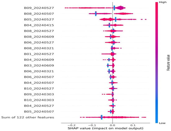
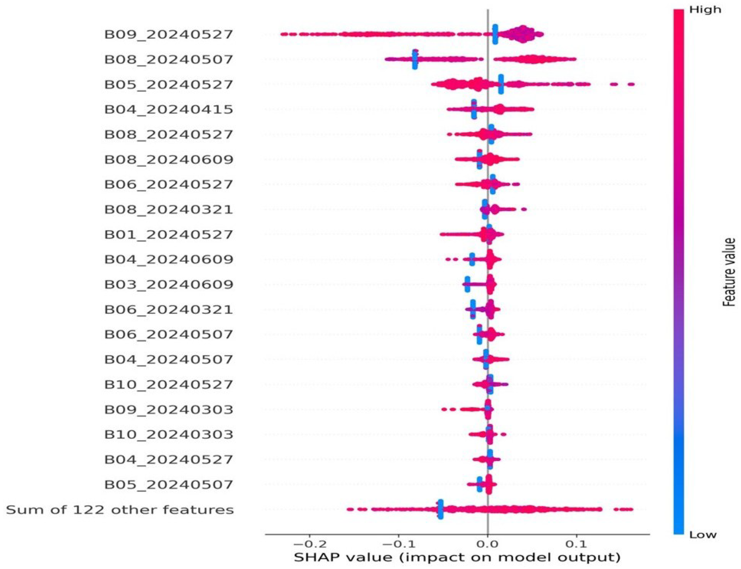
In Figure 11, the SWIR-1 (B09), NIR-narrow (B08), NIR (B07), and red-edge bands (B04–B06) dominate the model, mostly pushing predictions upward when their values are high, while visible bands and SWIR-2 contribute less. Importance clusters around scenes from 27 May 2024 and 9 June 2024, indicating that late-May/early-June phenology is most informative; the “Sum of 122 other features” is near zero.

Figure 11. SHAP summary (RF, Sentinel-only).

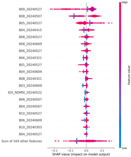
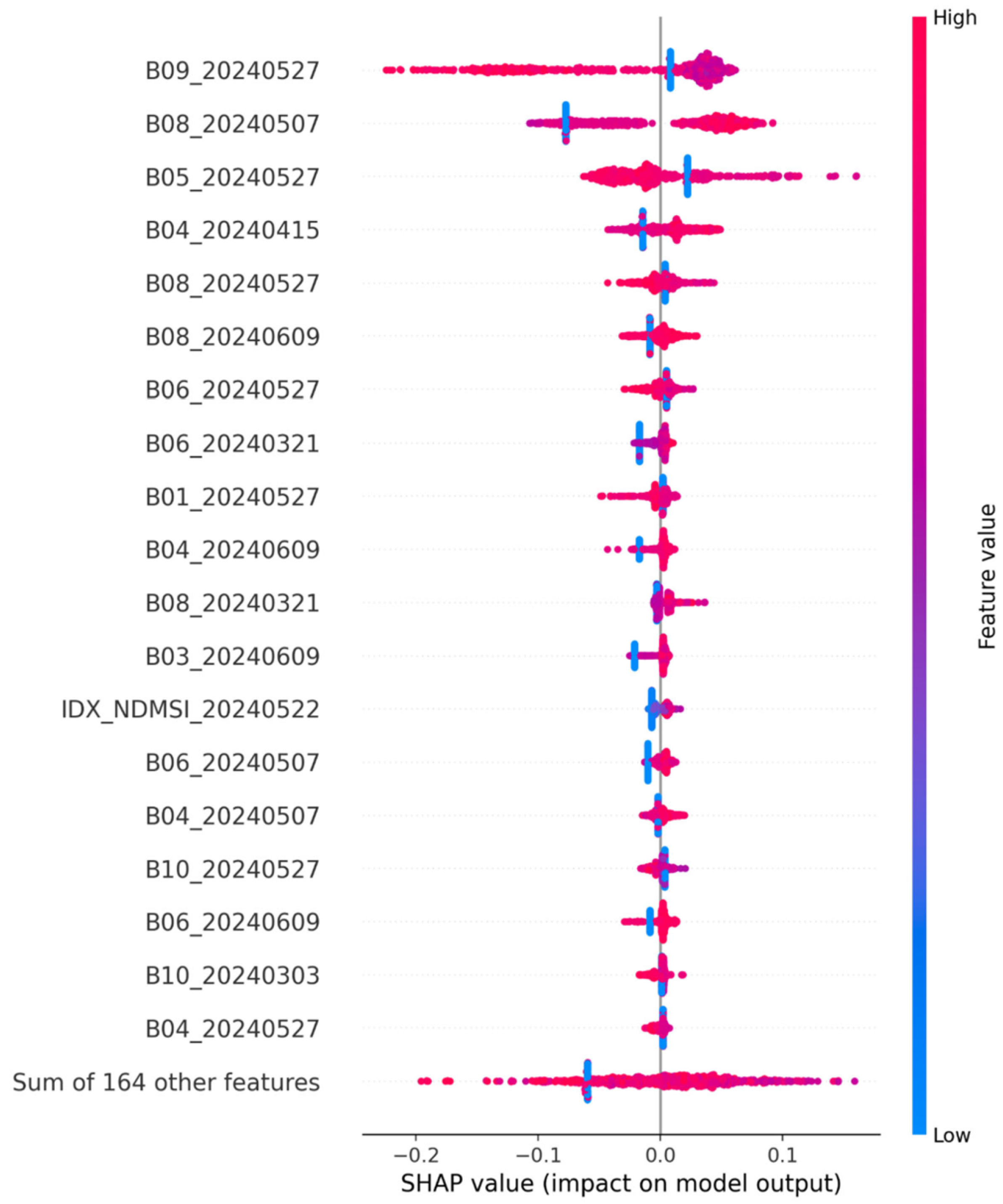
As shown in Figure 12, the bands with the highest global impacts remain SWIR-1 (B09), NIR-narrow (B08), red-edge (B04–B06), and NIR (B07)—especially from scenes on 2024-05-27 and 2024-05-07. High values (pink) generally push predictions upward, while low values (blue) pull them down. The added index NDMSI (2024-05-22) appears among the top features, but with a smaller effect than the leading bands. The aggregated “Sum of 164 other features” is near zero.

Figure 12. SHAP summary (RF, Sentinel-only + indices).

4. Discussion

The comparative analysis of feature configurations yielded a key finding for operational yield estimation: the Sentinel-only (SO) and Sentinel+Indices (SI) setups demonstrated nearly identical predictive performance across all evaluated metrics, with RF achieving $R^2\approx 0.91$, MAPE = $7.90\%$, and RMSE = $45.15$ kg decare⁻¹ under the SO configuration. The formal statistical comparison further confirmed that no significant difference existed between the two Sentinel-based configurations ($p_{\mathrm{holm}}=0.523$), while both were significantly superior to the Indices-only setup. This finding aligns with recent evidence from Mediterranean cereal systems, where high-capacity non-linear learners have shown that raw spectral data can encode biophysical information more effectively than derived vegetation indices [13,18,21]. For instance, Bebie et al. [13] demonstrated on the Thessaly plain in Greece that RF models using all Sentinel-2 bands achieved $R^2>0.91$, emphasizing that the full spectral resolution of Sentinel-2 allows machine learning models to extract complex features without the information loss inherent in pre-calculated ratios. Similarly, Mancini et al. [21] found that utilizing the full spectral range through deep learning architectures outperformed models restricted to specific indices.

SHAP analysis conducted on the best-performing configuration offers a mechanistic interpretation of this result. Model predictions were primarily driven by a subset of spectral bands—most notably the SWIR-1, NIR-narrow, and red-edge bands—observed during the late grain-filling and maturity stages, from late May to early June. The physiological relevance of these regions is well supported: the red-edge bands (B5, B6) are highly sensitive to chlorophyll and nitrogen status [36], while SWIR bands reflect canopy water content and senescence dynamics [1]. Our results confirm that the model identified these critical bands during the optimal phenological window, a timing consistency also reported in Turkey ($R^2=0.86$) [40] and Spain ($R^2=0.83$) [5]. The marginal contribution of derived indices further supports the interpretation that raw multi-temporal bands already encode the necessary biophysical proxies, rendering explicit index computation largely redundant within the scope of this study.

Crucially, the implementation of a strict Leave-One-Field-Out (LOFO) cross-validation protocol addresses a major criticism in the literature regarding spatial autocorrelation [27,28,39]. Many studies relying on random pixel-level splits likely overestimate predictive performance owing to strong spatial dependencies among neighboring observations [28,29]. By contrast, our LOFO approach ensures that reported metrics reflect genuine out-of-sample generalization to unseen agricultural parcels [27,39]. This level of methodological rigor is essential for transitioning from experimental pilots to operational decision-support tools in fragmented Mediterranean landscapes [14].

The primary methodological conclusion is that, within the spatial and seasonal scope of this study, raw multi-temporal Sentinel-2 spectral bands were sufficient to achieve high-accuracy prediction of wheat yields without the need to derive additional vegetation indices. This streamlines the processing pipeline by reducing feature engineering requirements and computational overhead [13,16]. However, because the current dataset covers a single growing season and nine commercial fields, this conclusion should be interpreted as evidence of operational potential rather than broad geographic or multi-seasonal sufficiency. Nevertheless, the achieved accuracy is comparable to that of top-performing models reported in Morocco ($R^2=0.93$) [41,42] and Tunisia ($R^2=0.91$) [17]. In subsequent phases, the methodology will be expanded to incorporate meteorological variables and soil characteristics, as data-fusion approaches have shown the potential to further improve model robustness across contrasting climatic conditions [1,2,20].

References

- Zeng, X.; Han, D.; Tansey, K.; Wang, P.; Pei, M.; Li, Y.; Li, F.; Du, Y. An Interpretable Wheat Yield Estimation Model Using Time Series Remote Sensing Data and Considering Meteorological and Soil Influences. Remote Sens. 2025, 17, 3192. [Google Scholar] [CrossRef] [Scilit]
- Kheir, A.M.S.; Govind, A.; Nangia, V.; Devkota, M.; Elnashar, A.; Omar, M.E.D.M.; Feike, T. Developing Automated Machine Learning Approach for Fast and Robust Crop Yield Prediction Using a Fusion of Remote Sensing, Soil, and Weather Dataset. Environ. Res. Commun. 2024, 6, 041005. [Google Scholar] [CrossRef] [Scilit]
- Chen, P.; Li, Y.; Liu, X.; Wang, J.; Jiang, Y.; Zhang, H.; Guo, Y.; Li, Z.; Qin, Y.; Deng, G.; et al. Improving Yield Prediction Based on Spatio-Temporal Deep Learning Approaches for Winter Wheat: A Case Study in Jiangsu Province, China. Comput. Electron. Agric. 2023, 213, 108201. [Google Scholar] [CrossRef] [Scilit]
- Segarra, J.; González-Torralba, J.; Aranjuelo, Í.; Araus, J.L.; Kefauver, S.C. Estimating Wheat Grain Yield Using Sentinel-2 Imagery and Exploring Topographic Features and Rainfall Effects on Wheat Performance in Navarre, Spain. Remote Sens. 2020, 12, 2278. [Google Scholar] [CrossRef] [Scilit]
- Segarra, J.; Araus, J.L.; Kefauver, S.C. Farming and Earth Observation: Sentinel-2 Data to Estimate Within-Field Wheat Grain Yield. Int. J. Appl. Earth Obs. Geoinf. 2022, 107, 102697. [Google Scholar] [CrossRef] [Scilit]
- Gavasso-Rita, Y.L.; Papalexiou, S.M.; Li, Y.; Elshorbagy, A.; Li, Z. Crop Models and Their Use in Assessing Crop Production and Food Security: A Review. Food Energy Secur. 2023, 12, e503. [Google Scholar] [CrossRef] [Scilit]
- Wajid, A.; Hussain, K.; Ilyas, A.; Habib-ur Rahman, M.; Shakil, Q.; Farooq, M.; Ahmad, A. Crop Models: Important Tools in Decision Support System to Manage Wheat Production under Vulnerable Environments. Agriculture 2021, 11, 1166. [Google Scholar] [CrossRef] [Scilit]
- Mihret, Y.C.; Ketsela, G.M.; Mintesinot, S.M. Implementation and Application of APSIM for Crop Modelling in Ethiopia: A Comprehensive Review. Heliyon 2024, 10, e31612. [Google Scholar] [CrossRef] [Scilit] [PubMed]
- Gabbrielli, M.; Allegrezza, M.; Ragaglini, G.; Manco, A.; Vitale, L. A Review of the Main Process-Based Approaches for Modeling N2O Emissions from Agricultural Soils. Horticulturae 2024, 10, 98. [Google Scholar] [CrossRef] [Scilit]
- Wimalasiri, E.M.; Ariyachandra, S.P.; Jahanshiri, E.; Muttil, N.; Rathnayake, U. Process-Based Crop Models in Soil Research: A Bibliometric Analysis. Soil Syst. 2023, 7, 43. [Google Scholar] [CrossRef] [Scilit]
- Sachin, G.; Mohammed Ahamed, J.; Nagajothi, K.; Rana, M.; Murugan, B.S. Automation of the DSSAT Crop Growth Simulation Model. Int. Arch. Photogramm. Remote Sens. Spat. Inf. Sci. 2019, XLII-3/W6, 251–256. [Google Scholar] [CrossRef] [Scilit]
- Gkologkinas, G.D.; Ntouros, K.; Protopapadakis, E.; Rallis, I. A Comparative Analysis of U-Net Architectures with Dimensionality Reduction for Agricultural Crop Classification Using Hyperspectral Data. Algorithms 2025, 18, 588. [Google Scholar] [CrossRef] [Scilit]
- Bebie, M.; Cavalaris, C.; Kyparissis, A. Assessing Durum Wheat Yield Through Sentinel-2 Imagery: A Machine Learning Approach. Remote Sens. 2022, 14, 3880. [Google Scholar] [CrossRef] [Scilit]
- El Imanni, H.S.; El Harti, A.; El Iysaouy, L. Wheat Yield Estimation Using Remote Sensing Indices Derived from Sentinel-2 Time Series and Google Earth Engine in a Highly Fragmented and Heterogeneous Agricultural Region. Agronomy 2022, 12, 2853. [Google Scholar] [CrossRef] [Scilit]
- Ishaq, R.A.F.; Zhou, G.; Jing, G.; Shah, S.R.A.; Ali, A.; Imran, M.; Jiang, H.; ur Rehman, O. Geospatial Robust Wheat Yield Prediction Using Machine Learning and Integrated Crop Growth Model and Time-Series Satellite Data. Remote Sens. 2025, 17, 1140. [Google Scholar] [CrossRef] [Scilit]
- European Space Agency. Sentinel-2 User Handbook, 2015. Issue 1, Rev. 2. Available online: https://sentinels.copernicus.eu/documents/247904/685211/Sentinel-2_User_Handbook (accessed on 28 March 2026).
- Mehdaoui, R.; Anane, M. Exploitation of the Red-Edge Bands of Sentinel 2 to Improve the Estimation of Durum Wheat Yield in Grombalia Region (Northeastern Tunisia). Int. J. Remote Sens. 2020, 41, 8043–8066. [Google Scholar] [CrossRef] [Scilit]
- Bebie, M.; Kyparissis, A. A Comparative Analysis of Machine Learning and Vegetation Index-Based Modeling Approaches for Durum Wheat Yield Assessment Using Sentinel-2 Imagery. In Proceedings of the Remote Sensing for Agriculture, Ecosystems, and Hydrology XXVI; SPIE: Bellingham, WA USA, 2024; Volume 13191, p. 1319107. [Google Scholar] [CrossRef] [Scilit]
- Cavalaris, C.; Megoudi, S.; Maxouri, M.; Anatolitis, K.; Sifakis, M.; Levizou, E.; Kyparissis, A. Modeling of Durum Wheat Yield Based on Sentinel-2 Imagery. Agronomy 2021, 11, 1486. [Google Scholar] [CrossRef] [Scilit]
- Uribeetxebarria, A.; Castellón, A.; Aizpurua, A. Optimizing Wheat Yield Prediction Integrating Data from Sentinel-1 and Sentinel-2 with CatBoost Algorithm. Remote Sens. 2023, 15, 1640. [Google Scholar] [CrossRef] [Scilit]
- Mancini, A.; Solfanelli, F.; Coviello, L.; Martini, F.M.; Mandolesi, S.; Zanoli, R. Time Series from Sentinel-2 for Organic Durum Wheat Yield Prediction Using Functional Data Analysis and Deep Learning. Agronomy 2024, 14, 109. [Google Scholar] [CrossRef] [Scilit]
- Ntouros, K.; Papatheodorou, K.; Gkologkinas, G.; Drimzakas-Papadopoulos, V. A Python Framework for Crop Yield Estimation Using Sentinel-2 Satellite Data. Earth 2025, 6, 15. [Google Scholar] [CrossRef] [Scilit]
- Bian, C.; Shi, H.; Wu, S.; Zhang, K.; Wei, M.; Zhao, Y.; Sun, Y.; Zhuang, T.; Zhang, X.; Chen, S. Prediction of Field-Scale Wheat Yield Using Machine Learning Method and Multi-Spectral UAV Data. Remote Sens. 2022, 14, 1474. [Google Scholar] [CrossRef] [Scilit]
- Tuğaç, M.G.; Özbayoğlu, A.M.; Torunlar, H.; Karakurt, E. Wheat Yield Prediction with Machine Learning Based on MODIS and Landsat NDVI Data at Field Scale. Int. J. Environ. Geoinf. 2022, 9, 172–184. [Google Scholar] [CrossRef] [Scilit]
- Huber, F.; Yushchenko, A.; Stratmann, B.; Steinhage, V. Extreme Gradient Boosting for Yield Estimation Compared with Deep Learning Approaches. Comput. Electron. Agric. 2022, 202, 107346. [Google Scholar] [CrossRef] [Scilit]
- Mateo-Sanchis, A.; Adsuara, J.E.; Piles, M.; Campos-Taberner, M.; García-Haro, F.J.; Camps-Valls, G. Interpretable Long Short-Term Memory Networks for Crop Yield Estimation. IEEE Geosci. Remote Sens. Lett. 2023, 20, 2501105. [Google Scholar] [CrossRef] [Scilit]
- Killeen, P.; Kiringa, I.; Yeap, T.; Branco, P. Corn Grain Yield Prediction Using UAV-Based High Spatiotemporal Resolution Imagery, Machine Learning, and Spatial Cross-Validation. Remote Sens. 2024, 16, 683. [Google Scholar] [CrossRef] [Scilit]
- Radočaj, D.; Jurišić, M.; Gašparović, M.; Plaščak, I. A Comparative Assessment of Regular and Spatial Cross-Validation in Subfield Machine Learning Prediction of Maize Yield from Sentinel-2 Phenology. Eng 2025, 6, 270. [Google Scholar] [CrossRef] [Scilit]
- Habibi, L.N.; Matsui, T.; Tanaka, T.S. Critical Evaluation of the Effects of a Cross-Validation Strategy and Machine Learning Optimization on the Prediction Accuracy and Transferability of a Soybean Yield Prediction Model Using UAV-Based Remote Sensing. J. Agric. Food Res. 2024, 16, 101096. [Google Scholar] [CrossRef] [Scilit]
- Stiller, D.; Ottinger, M.; Leinenkugel, P. Improving Spatial Transferability of Deep Learning Segmentation Models for Small-Field Crop Yield Prediction. ISPRS Open J. Photogramm. Remote Sens. 2024, 12, 100058. [Google Scholar] [CrossRef] [Scilit]
- Mateo-Sanchis, A.; Piles, M.; Muñoz-Marí, J.; Adsuara, J.E.; Pérez-Suay, A.; Camps-Valls, G. Learning Main Drivers of Crop Progress and Failure in Europe with Interpretable Machine Learning. Int. J. Appl. Earth Obs. Geoinf. 2021, 104, 102574. [Google Scholar] [CrossRef] [Scilit]
- Lundberg, S.M.; Lee, S.I. A Unified Approach to Interpreting Model Predictions. In NIPS’17: Proceedings of the 31st International Conference on Neural Information Processing Systems; Curran Associates, Inc.: Red Hook, NY, USA, 2017; pp. 4768–4777. [Google Scholar]
- Molnar, C. Interpretable Machine Learning: A Guide for Making Black Box Models Explainable, 2nd ed.; Lulu Press, Inc.: Morrisville, NC, USA, 2022; Available online: https://christophm.github.io/interpretable-ml-book/ (accessed on 28 March 2026).
- Kumar, C.; Dhillon, J.; Huang, Y.; Reddy, K. Explainable Machine Learning Models for Corn Yield Prediction Using UAV Multispectral Data. Comput. Electron. Agric. 2025, 231, 109990. [Google Scholar] [CrossRef] [Scilit]
- Dey, A.; Saha, A.; Sarkar, S.; Mondal, S.; Mitra, S. An Explainable AI-Driven Feature Reduction Framework for Enhanced Agricultural Yield Prediction. In Proceedings of the EGU General Assembly 2025, EGU25-7965, Vienna, Austria, 27 April–2 May 2025. [Google Scholar] [CrossRef] [Scilit]
- Shi, B.; Chen, X.; Guo, Y.; Liu, L.; Li, P.; Chang, Q. Multi-Source Feature Selection and Explainable Machine Learning Approach for Mapping Nitrogen Balance Index in Winter Wheat Based on Sentinel-2 Data. Remote Sens. 2025, 17, 3196. [Google Scholar] [CrossRef] [Scilit]
- Drimzakas-Papadopoulos, V.; Ntouros, K.; Papatheodorou, C.; Konstantinidis, A. Use of UAVs’ multispectral images for sugar beet cultivars discrimination and yield estimation. J. Cent. Eur. Agric. 2024, 25, 1135–1147. [Google Scholar] [CrossRef] [Scilit]
- Kopsiaftis, G.; Protopapadakis, E.; Voulodimos, A.; Doulamis, N.; Mantoglou, A. Gaussian process regression tuned by bayesian optimization for seawater intrusion prediction. Comput. Intell. Neurosci. 2019, 2019, 2859429. [Google Scholar] [CrossRef] [Scilit]
- Alshihabi, O.; Persson, K.; Söderström, M. Easy yield mapping for precision agriculture. Acta Agric. Scand. Sect. B—Soil Plant Sci. 2024, 74, 2411950. [Google Scholar] [CrossRef] [Scilit]
- Civelek, N.; Genç, L.; Akçay, Ö. Wheat yield prediction for sustainable food security using Sentinel-2 and machine learning. Turk. J. Remote Sens. 2026, 8, 1–24. [Google Scholar] [CrossRef] [Scilit]
- El Ayyadi, M.; Meghraoui, K.; El Hamdani, M.; Bensiali, S.; Lozzi, A.; Sebari, I. STAF-Net: An Innovative Framework for Wheat Yield Prediction. Int. Arch. Photogramm. Remote Sens. Spat. Inf. Sci. 2026, 48, 45–53. [Google Scholar] [CrossRef] [Scilit]
- Chahbi-Bellakanji, A.; Shil, E.; Khlif, M.; Zribi, M.; Lili-Chabaane, Z. Early cereal yield prediction using machine learning and Sentinel-1 & Sentinel-2 satellite data. Eur. J. Remote Sens. 2025, 58, 2558614. [Google Scholar]
Disclaimer/Publisher’s Note: The statements, opinions and data contained in all publications are solely those of the individual author(s) and contributor(s) and not of MDPI and/or the editor(s). MDPI and/or the editor(s) disclaim responsibility for any injury to people or property resulting from any ideas, methods, instructions or products referred to in the content. |
© 2026 by the authors. Licensee MDPI, Basel, Switzerland. This article is an open access article distributed under the terms and conditions of the Creative Commons Attribution (CC BY) license.