Graph-Contrastive Pretraining for Payload-Free Encrypted-Traffic Intrusion Detection: Cross-Dataset OOD Transfer with Frozen Artifacts

Abstract

Encrypted transport increasingly limits the visibility required by intrusion detection systems (IDS), motivating payload-free learning from flow statistics and protocol metadata. We introduce GCP, a graph-contrastive pretraining framework that casts flows as nodes in a sparse graph and learns transferable node embeddings via an InfoNCE-style objective with graph-specific augmentations. The learned encoder is evaluated through frozen-embedding linear probing and cross-dataset out-of-domain (OOD) transfer, within a fully scripted pipeline that freezes run manifests and artifacts to make every reported number traceable and reproducible. Experiments cover enterprise IDS and encrypted DNS/DoH traffic using CICIDS2017, UNSW-NB15, and DoH-Combined at three label granularities (L1/L2/L3), for both binary detection (y) and finer-grained targets ($y_{\mathrm{multi}}$), aggregated over five fixed split seeds with 95% confidence intervals. Results show that GCP yields a pronounced in-domain advantage on UNSW-NB15 for y (Macro-F1 $\approx 0.993$) while substantially reducing false-alarm rate (FAR $\approx 0.013$) compared with strong tabular baselines. In feature-separable regimes (CICIDS2017 and DoH L1/L2), boosted-tree and supervised baselines remain difficult to surpass, but ablations confirm that graph structure alone is insufficient without contrastive pretraining. OOD transfer is strongly source–target dependent, with the most reliable transfer within closely related DoH domains, highlighting dataset shift as a first-class evaluation criterion for encrypted-traffic IDS.

1. Introduction

The rapid encryption of network communications has reshaped the operational landscape of intrusion detection. Payload-centric inspection becomes infeasible under ubiquitous TLS, while encrypted DNS—and in particular DNS over HTTPS (DoH)—further reduces visibility into intent and destinations [1]. As a consequence, modern intrusion detection systems (IDS) must rely on metadata, flow statistics, and behavioral signals that remain observable without decryption, while still achieving actionable false-alarm levels in highly imbalanced environments [2].

A dominant line of work addresses encrypted-traffic detection by engineering tabular features from packet/flow summaries and learning classifiers on a per-dataset basis, often with strong performance when training and test distributions are closely matched [3,4]. However, IDS deployment is repeatedly challenged by dataset shift: changes in capture environment, benign usage patterns, attack tooling, and labeling conventions can severely reduce generalization [5,6]. This is particularly acute for encrypted traffic, where discriminative cues may be subtle and entangled with context.

In parallel to IDS-centric approaches, the cyber–physical security literature has studied deception attacks under communication constraints using adaptive event-triggered mechanisms and robust/fuzzy control. These works complement IDS perspectives by formalizing attack-dependent scheduling and tracking under adversarial perturbations in networked systems [7,8].

In addition, the literature frequently suffers from limited end-to-end reproducibility: when preprocessing, splits, and intermediate artifacts are not traceable, it becomes difficult to attribute gains to modeling advances rather than to leakage or undocumented choices. Our recent deterministic and leakage-aware benchmarking for IDS highlights how methodological rigor can materially affect conclusions [9].

In this work, we argue that two ingredients are jointly required for progress on payload-free encrypted-traffic IDS: (i) a representation that captures relational structure beyond independent flows, and (ii) a learning signal that can exploit abundant unlabeled data and transfer across domains. We therefore cast traffic samples as nodes in a graph and learn representations using a contrastive self-supervised objective. Contrastive learning has demonstrated strong representation quality in other domains [10,11], and graph self-supervised learning provides practical mechanisms to construct invariances through augmentations and view agreement [12,13].

Building on these principles, we propose GCP (Graph-Contrastive Pretraining), a payload-free pretraining framework that produces transferable node embeddings, which are then evaluated with lightweight probing and cross-dataset transfer.

We evaluate GCP in a strictly reproducible pipeline (Section 2) over five benchmark settings spanning enterprise IDS and DoH traffic: CICIDS2017 [14], UNSW-NB15 [15], and DoH-Combined at three label granularities derived from CIRA-CIC-DoHBrw-2020 [16]. We consider both binary detection (y) and a finer-grained target ($y_{\mathrm{multi}}$), and we report results over five seeds with confidence intervals. Because IDS data are typically skewed, we interpret ROC/PR jointly and emphasize threshold-independent measures appropriate for imbalance, including AUPR and operational false-alarm behavior [17,18].

Our comparisons include:

1.

GCP with frozen-encoder probing;

2.

a supervised message-passing GNN baseline grounded in standard GNN architectures [19,20,21];

3.

an SSL ablation without contrastive learning;

4.

and strong tabular baselines (XGBoost and MLP), which remain competitive in separable regimes.

The paper makes three contributions:

(i)

We formulate a payload-free graph representation and a contrastive pretraining scheme (GCP) for encrypted-traffic intrusion detection, grounded in established contrastive and graph-SSL practice [10,11,13];

(ii)

we provide a cross-dataset evaluation that explicitly measures out-of-domain (OOD) transfer via frozen artifacts and lightweight probing, complementing in-domain performance with generalization evidence [5];

(iii)

and we operationalize end-to-end reproducibility by freezing the exact run manifests, configurations, and intermediate artifacts used to generate every table and figure, extending deterministic IDS benchmarking principles to graph-based self-supervised learning [9].

The results in Section 3 substantiate that contrastive pretraining is the enabling component: simply using graphs is not sufficient without an appropriate self-supervised signal, and transfer behavior can be systematically characterized across source–target pairs.

2. Methodology

2.1. Overview and Reproducible Pipeline

Our methodology is implemented as a fully scripted and reproducible pipeline. Raw and intermediate artifacts are materialized under data/processed/, experiment runs are stored under results/runs/ (each run includes config.yaml and meta.json), and the exact subset of runs used in the paper is frozen under results/paper/paper_grande/ (including frozen tables, figures, and manifests). This design guarantees that every number reported in tables/plots is traceable to a specific run directory and configuration.

2.2. Datasets, Label Spaces, and Prediction Targets

We evaluate five benchmark settings spanning enterprise and IoT traffic: (i) CICIDS2017 [14], (ii) UNSW-NB15 (Feature) [15], and (iii) DoH-Combined at three label granularities L1/L2/L3 derived from CIRA-CIC-DoHBrw-2020 [16]. For each setting we define two prediction targets: a binary target y (Normal vs. Attack) and a multi-class target $y_{\mathrm{multi}}$ capturing finer-grained attack categories. Label harmonization and target definitions are centralized in configuration files (e.g., configs/label_map.yaml) to ensure consistent semantics across all phases.

2.3. Tabular Preprocessing and Flow Materialization

For each dataset/setting, we materialize a canonical flow table flows_v1.parquet (plus dataset metadata such as label_counts.csv when available) under data/processed/ <dataset>/.... This step standardizes column naming, resolves missing values, and applies deterministic encodings so that downstream graph construction and tabular baselines consume the same feature space. For UNSW-NB15, we use the feature representation (the one used throughout the paper) under data/processed/unsw-nb15/feature/.

2.4. Graph Construction and Stored Graph Assets

Each tabular flow dataset is transformed into a sparse graph representation to enable message-passing models. We store the graph explicitly under data/processed/<dataset>/ <variant>/graph_v2/ as: (i) adjacency in COO form edge_index.npy, (ii) optional relation typing edge_type.npy, (iii) node table nodes.parquet, and (iv) graph metadata/statistics (meta.json, stats.json). Node features are split into numeric and categorical tensors: x_num.npy and x_cat.npy, with categorical dictionaries in x_cat_maps.json. Targets are stored as y.npy and y_multi.npy. This explicit materialization is essential for reproducibility and for enabling both in-domain evaluation and OOD transfer (Section 2.7).

2.5. Seeded Train/Validation/Test Splits

We use a fixed set of five seeds $\{0,42,1337,2026,9999\}$ to generate train/validation/test partitions. For graph-based experiments, each seed corresponds to an explicit split directory data/processed/<dataset>/<variant>/graph_v2/splits/seed<k>/ containing train_nodes.npy, val_nodes.npy, and test_nodes.npy (plus meta.json). For tabular experiments, we additionally materialize ID-based splits (e.g., train_ids.parquet, val_ids.parquet, test_ids.parquet) when available. All reported results aggregate performance across the five seeds.

2.6. Models and Training Objectives

Model configurations and hyperparameters (shared across datasets unless noted) are summarized in

Table 1. Model configurations (shared across datasets unless noted). Values shown for GCP/GNN-Sup/SSL include those found in run artifacts plus a proposed default completion for fields not exported, to make the methodology fully specified and reproducible.

Model/Component	Key Setup/Hyperparameters
GCP encoder $f_{\theta }$	Backbone: GraphSAGE-mean with L = 2 layers, hidden dim hidden = 128, dropout p = 0.2; neighbor sampling neigh_k = 10; categorical embedding cat_emb = 16. Batch nodes batch_nodes = 4096; device cpu. Graph inputs: cicids2017/graph_v2, unsw-nb15/argus/graph_v2, unsw-nb15/feature/graph_v3, doh-combined/l1|l2|l3/graph_v2.
Projection head $g_{\varphi }$	2-layer MLP: 128 → 128 → 64 (proj_dim = 64), activation ReLU, dropout 0.0, output L2-normalized.
Contrastive objective	InfoNCE with cosine similarity; temperature tau = 0.2; in-batch negatives over batch_nodes = 4096.
Graph augmentations	Feature masking feat_mask_p = 0.15; edge dropout edge_drop_p = 0.2; subgraph cap max_nodes in {50,000, 200,000}; edge budget per epoch edge_sample in {2,000,000, 3,000,000} (fallback 2 for tiny graphs).
Pretraining optimization	Optimizer Adam; learning rate lr = 0.001; weight decay $1\times {10}^{-4}$ epochs 5 (short ablations may use 1 or 3); gradient clipping 1.0; early stopping on val_loss with patience 10; embeddings saved as float16 (save_embed_dtype = float16).
Linear probe (frozen encoder)	Binary y: logistic regression (solver = lbfgs), C = 1.0, max_iter = 2000, class_weight = balanced. Multiclass $y_{\mathrm{multi}}$: multinomial logistic regression (solver = lbfgs), C = 1.0, max_iter = 2000. For both: random_state = seed, features standardized (StandardScaler) on train split only.
GNN-Sup (end-to-end)	Backbone: GraphSAGE-mean with L = 2 layers; hidden = 256, dropout = 0.2, epochs = 50, lr = 0.001, weight_decay = $1\times {10}^{-4}$, batch_nodes = 512, neigh_k = 10, cat_emb = 16, early stopping patience = 3, max_train_nodes = 200,000, deterministic = true.
SSL no-contrast	ssl_nocontrast_graphmae_lite (masked reconstruction): encoder backbone GraphSAGE-mean, n_layers = 2, hidden = 128, dropout = 0.2, batch_nodes = 512, neigh_k = 10, mask ratio mask_ratio = 0.3. Pretraining: pre_epochs = 50, pre_lr = 0.001, pre_wd = $1\times {10}^{-4}$, pre_patience = 4. Probe: probe_epochs = 50, probe_lr = 0.01, probe_patience = 5. Device: cpu.
Tabular-XGB	XGBoost (tree_method = hist): n_estimators = 500, max_depth = 8, learning_rate = 0.05, subsample = 0.8, colsample_bytree = 0.8, min_child_weight = 1, gamma = 0, reg_lambda = 1.0, reg_alpha = 0.0; early stopping early_stopping_rounds = 50 on validation. Seeds: {0,42,1337,2026,9999}; deterministic training enabled. Datasets/targets: cicids2017 (y, $y_{\mathrm{multi}}$), unsw-nb15-feature (y, $y_{\mathrm{multi}}$), doh-combined-l1 (y), doh-combined-l2 (y), doh-combined-l3 ($y_{\mathrm{multi}}$).
Tabular-MLP	MLP: layers [512, 256], activation ReLU, dropout 0.2; optimizer Adam, lr = 0.001, weight_decay = $1\times {10}^{-4}$, batch size 1024, epochs 50, early stopping patience 10 on validation. Seeds: {0,42,1337,2026,9999}; deterministic training enabled.

. Unless explicitly stated otherwise, the same settings are used for CICIDS2017, UNSW-NB15 (Feature), and DoH-Combined (L1/L2/L3).

We compare three families of approaches, aligned with the experimental structure discussed in Section 3.

• Graph-Contrastive Pretraining (GCP).

GCP trains a message-passing GNN encoder $f_{\theta }(·)$ to produce node embeddings via a contrastive objective over two stochastically augmented views of the same graph, following the contrastive learning paradigm popularized by SimCLR/CPC and adapted to graphs by GraphCL [10,11,13]. Concretely, for each node we obtain two embeddings $({\mathbf{z}}_i,{\mathbf{z}}_i^{\prime })$ from two graph views and optimize an InfoNCE-style objective that increases agreement between positives (same node across views) and decreases agreement to negatives (other nodes in the batch) [10,11]. We use standard graph augmentations as in GraphCL (e.g., stochastic feature masking and structural perturbations) [13]. To connect with widely used graph self-supervision baselines, we also reference Deep Graph Infomax (DGI) as a conceptual anchor for mutual-information-based graph representation learning [12].

• Linear-probe evaluation on frozen embeddings.

After pretraining, we freeze $f_{\theta }$ and train a lightweight classifier $g(·)$ on top of embeddings using only labeled nodes from the training split. This protocol isolates representation quality from end-to-end supervised tuning and is the primary evaluation strategy throughout the paper (including OOD transfer).

• Supervised GNN baseline (GNN-Sup).

As a strong graph baseline, we train a supervised message-passing GNN end-to-end on labeled nodes using the same graph assets and splits as GCP. Architecturally, this family follows standard GNN building blocks such as GCN/GAT-style message passing [19,20,21].

• SSL without contrast (reconstruction baseline).

To quantify the marginal value of contrastive learning, we include a self-supervised baseline that removes the contrastive term and instead uses a reconstruction-style objective (implemented as a masked autoencoding variant in our pipeline). This baseline shares the same graph inputs and is evaluated with the same linear-probe protocol.

• Tabular baselines.

We evaluate tabular models directly on the flow features to contextualize gains from graph structure and pretraining. Our main tabular baselines are gradient-boosted decision trees (XGBoost) [3] and a multilayer perceptron (MLP). Tabular results are aggregated per dataset and target and exported as paper-ready .tex tables under results/paper/paper_grande/tables/.

2.7. In-Domain Evaluation and OOD Transfer

• In-domain protocol.

For each dataset/setting and each seed, we train the representation model (GCP pretraining or supervised GNN) using the training split, select model checkpoints/hyperparameters using the validation split, and report final metrics on the test split. For GCP, the classifier is trained only on frozen embeddings produced by the pretrained encoder.

• OOD transfer protocol.

To evaluate cross-domain generalization, we pretrain the GCP encoder on a source dataset and then apply the frozen encoder to a different target dataset to compute target-node embeddings (exported by the pipeline under OOD-specific run directories). We then fit a linear probe on the target training split and evaluate on the target test split. This protocol operationalizes dataset shift and domain transfer in IDS settings [5,6] and is the basis for the OOD analyses discussed in Section 3.

2.8. Metrics and Uncertainty Estimation

We report Accuracy, Macro-F1, AUROC, AUPR, and False Alarm Rate (FAR). AUROC and AUPR follow standard definitions; AUPR is emphasized under class imbalance [17,18]. FAR captures the operational cost of false alerts and is reported when computable from the available confusion statistics [2]. Uncertainty is summarized as mean ±95% confidence interval across the five seeds. With $n=5$ seeds, we use the Student-t interval $\overline{x}\pm t_{0.975,n-1}s/\sqrt{n}$ [22]. All ROC/PR curves and bar plots are generated from seed-wise exported points and aggregated means, ensuring exact consistency between plotted curves and tabulated scalar metrics.

2.9. Implementation Details and Artifact Traceability

All experiments are implemented in Python using PyTorch [23] and PyTorch Geometric [24], with tabular baselines and probes implemented using scikit-learn [25]. Data processing relies on NumPy and pandas [26,27]. For each run, the pipeline stores config.yaml and meta.json (including seed, dataset identifiers, and paths), plus model outputs and evaluation artifacts (e.g., confusion matrices, ROC/PR points, and summary CSVs). Paper-ready tables (.tex) and figures (.png, plus inline .tex includes) are frozen under results/paper/paper_grande/, while the underlying raw runs remain under results/runs/. This separation prevents accidental drift between late-stage paper editing and the frozen experimental evidence.

3. Discussion of Results

3.1. Scope, Evaluation Protocol, and How to Read the Tables/Figures

We discuss results over five benchmark datasets spanning enterprise IDS and encrypted DNS/DoH traffic: CICIDS2017 [14], UNSW-NB15 [15], and CIRA-CIC-DoHBrw-2020 [16]. We report metrics for a binary target y and a multi-class/multi-label target $y_{\mathrm{multi}}$ (where available), using five random seeds (0, 42, 1337, 2026, 9999) and 95% confidence intervals (CI) across seeds.

We compare: (i) GCP (our graph contrastive pretraining), inspired by contrastive SSL principles [10,11] and graph SSL practice [12,13]; (ii) a supervised GNN baseline (GNN-Sup), grounded in message-passing GNNs [19,20,21]; (iii) a self-supervised ablation without contrastive objective (SSL w/o contrast); and (iv) strong tabular baselines (XGBoost [3] and MLP).

For imbalanced detection problems, PR curves and AUPR are often more diagnostic than ROC/AUROC [18]. We therefore interpret ROC/PR jointly, and we use FAR as a practical false-alarm proxy (lower is better).

• What the results substantiate about novelty

The results support our central claim: a payload-free graph representation coupled with contrastive pretraining can yield competitive in-domain performance while enabling cross-dataset transfer with lightweight probing. In feature-separable regimes (CICIDS2017 and DoH-L1/L2), strong tabular baselines remain hard to beat, but the ablations (GNN-Sup and SSL w/o contrast) show that simply using graphs is insufficient without an appropriate pretraining signal. In addition, the OOD tables (

Table 2. Out-of-domain (OOD) transfer for binary classification (y): the GCP encoder is trained on the source dataset, frozen, then used to embed the target dataset where only a lightweight probe is trained. Each cell shows mean (top) and 95% CI (bottom). Bold indicates the best Macro-F1 for each target dataset (ties are bolded). Results for target DoH-Combined L3 are omitted here because the processed y distribution is single-class, making AUROC/AUPR/FAR undefined; they are reported separately in Appendix A Table A1.

Source Encoder	Target Dataset	Macro-F1	AUROC	AUPR	FAR
CICIDS2017	CICIDS2017	0.8194 [0.7679, 0.8538]	0.9281 [0.9221, 0.9339]	0.7115 [0.6921, 0.7341]	0.0937 [0.0619, 0.1311]
DoH-Combined L1	CICIDS2017	0.7845 [0.7186, 0.8407]	0.9260 [0.9192, 0.9312]	0.7233 [0.6962, 0.7448]	0.0958 [0.0666, 0.1312]
DoH-Combined L2	CICIDS2017	0.7803 [0.7411, 0.8313]	0.9190 [0.9082, 0.9273]	0.6855 [0.6640, 0.7114]	0.0923 [0.0606, 0.1404]
DoH-Combined L3	CICIDS2017	0.8225 [0.7974, 0.8637]	0.9268 [0.9213, 0.9344]	0.7478 [0.7253, 0.7779]	0.1053 [0.0641, 0.1366]
UNSW-NB15	CICIDS2017	0.8440 [0.8280, 0.8708]	0.9302 [0.9258, 0.9370]	0.7317 [0.7146, 0.7586]	0.1052 [0.0737, 0.1324]
CICIDS2017	DoH-Combined L1	0.9902 [0.9896, 0.9909]	0.9987 [0.9984, 0.9989]	0.9962 [0.9952, 0.9968]	0.0061 [0.0057, 0.0068]
DoH-Combined L1	DoH-Combined L1	0.9946 [0.9942, 0.9951]	0.9996 [0.9996, 0.9996]	0.9983 [0.9982, 0.9985]	0.0023 [0.0020, 0.0026]
DoH-Combined L2	DoH-Combined L1	0.9928 [0.9919, 0.9939]	0.9995 [0.9995, 0.9996]	0.9978 [0.9977, 0.9981]	0.0035 [0.0034, 0.0038]
DoH-Combined L3	DoH-Combined L1	0.9934 [0.9921, 0.9939]	0.9995 [0.9995, 0.9995]	0.9972 [0.9970, 0.9975]	0.0028 [0.0025, 0.0034]
UNSW-NB15	DoH-Combined L1	0.9936 [0.9933, 0.9938]	0.9995 [0.9995, 0.9996]	0.9983 [0.9982, 0.9984]	0.0030 [0.0025, 0.0035]
CICIDS2017	DoH-Combined L2	0.9915 [0.9858, 0.9940]	0.9999 [0.9999, 0.9999]	1.0000 [1.0000, 1.0000]	0.0228 [0.0129, 0.0430]
DoH-Combined L1	DoH-Combined L2	0.9876 [0.9826, 0.9921]	0.9998 [0.9998, 0.9998]	1.0000 [1.0000, 1.0000]	0.0326 [0.0155, 0.0518]
DoH-Combined L2	DoH-Combined L2	0.9875 [0.9826, 0.9910]	0.9998 [0.9998, 0.9998]	1.0000 [1.0000, 1.0000]	0.0323 [0.0195, 0.0513]
DoH-Combined L3	DoH-Combined L2	0.9905 [0.9850, 0.9934]	0.9999 [0.9998, 0.9999]	1.0000 [1.0000, 1.0000]	0.0252 [0.0158, 0.0454]
UNSW-NB15	DoH-Combined L2	0.9871 [0.9843, 0.9907]	0.9998 [0.9998, 0.9998]	1.0000 [1.0000, 1.0000]	0.0342 [0.0205, 0.0460]
CICIDS2017	UNSW-NB15	0.9157 [0.8773, 0.9301]	0.9550 [0.9539, 0.9559]	0.9782 [0.9776, 0.9786]	0.1797 [0.1471, 0.2212]
DoH-Combined L1	UNSW-NB15	0.9064 [0.8735, 0.9410]	0.9512 [0.9491, 0.9533]	0.9720 [0.9687, 0.9764]	0.1519 [0.1475, 0.1558]
DoH-Combined L2	UNSW-NB15	0.9064 [0.8725, 0.9414]	0.9512 [0.9490, 0.9531]	0.9721 [0.9685, 0.9762]	0.1513 [0.1461, 0.1550]
DoH-Combined L3	UNSW-NB15	0.9051 [0.8712, 0.9395]	0.9509 [0.9489, 0.9529]	0.9711 [0.9682, 0.9752]	0.1499 [0.1430, 0.1549]
UNSW-NB15	UNSW-NB15	0.9053 [0.8748, 0.9382]	0.9511 [0.9494, 0.9533]	0.9711 [0.9657, 0.9762]	0.1507 [0.1471, 0.1549]

and

Table 3. Out-of-domain (OOD) transfer for multi-class classification ($y_{\mathrm{multi}}$): the GCP encoder is trained on the source dataset, frozen, then used to embed the target dataset where only a lightweight probe is trained. Each cell shows mean (top) and 95% CI (bottom). Bold indicates the best Macro-F1 for each target dataset (ties are bolded). Results are reported across five fixed seeds (0, 42, 1337, 2026, 9999).

Source Encoder	Target Dataset	Macro-F1	AUROC	AUPR	FAR
CICIDS2017	CICIDS2017	0.1588 [0.1121, 0.1825]	0.5529 [0.5007, 0.5939]	0.1705 [0.1452, 0.1864]	0.1289 [0.0038, 0.3195]
DoH-Combined L1	CICIDS2017	0.1330 [0.1089, 0.1771]	0.5489 [0.4982, 0.6404]	0.1714 [0.1432, 0.2276]	0.1374 [0.0004, 0.3864]
DoH-Combined L2	CICIDS2017	0.1406 [0.1227, 0.1676]	0.5350 [0.4952, 0.5973]	0.1579 [0.1426, 0.1813]	0.1095 [0.0002, 0.2898]
DoH-Combined L3	CICIDS2017	0.1392 [0.1230, 0.1773]	0.5435 [0.4949, 0.5965]	0.1649 [0.1436, 0.1845]	0.1400 [0.0015, 0.3490]
UNSW-NB15	CICIDS2017	0.1399 [0.1051, 0.1653]	0.5857 [0.5470, 0.6123]	0.1848 [0.1715, 0.1968]	0.2545 [0.0499, 0.3815]
CICIDS2017	DoH-Combined L1	0.8240 [0.5260, 0.9233]	0.8471 [0.6492, 0.9174]	0.7538 [0.4913, 0.8498]	0.0187 [0.0038, 0.0340]
DoH-Combined L1	DoH-Combined L1	0.8371 [0.6992, 0.9249]	0.8689 [0.6963, 0.9606]	0.7897 [0.5660, 0.9154]	0.0154 [0.0029, 0.0440]
DoH-Combined L2	DoH-Combined L1	0.9297 [0.8778, 0.9582]	0.9594 [0.9291, 0.9781]	0.9190 [0.8568, 0.9494]	0.0155 [0.0030, 0.0268]
DoH-Combined L3	DoH-Combined L1	0.9353 [0.9245, 0.9585]	0.9578 [0.9347, 0.9707]	0.9176 [0.8655, 0.9301]	0.0161 [0.0033, 0.0296]
UNSW-NB15	DoH-Combined L1	0.4511 [0.4329, 0.4752]	0.6025 [0.5692, 0.6241]	0.3901 [0.3700, 0.4104]	0.0921 [0.0248, 0.1411]
CICIDS2017	DoH-Combined L2	0.4743 [0.4740, 0.4755]	0.5133 [0.5078, 0.5247]	0.9033 [0.9023, 0.9054]	0.9996 [0.9985, 1.0000]
DoH-Combined L1	DoH-Combined L2	0.5454 [0.5020, 0.5696]	0.5605 [0.5118, 0.5941]	0.9214 [0.9098, 0.9271]	0.8618 [0.7433, 0.9589]
DoH-Combined L2	DoH-Combined L2	0.5507 [0.5348, 0.5808]	0.5626 [0.5330, 0.5826]	0.9228 [0.9175, 0.9290]	0.8185 [0.7190, 0.9253]
DoH-Combined L3	DoH-Combined L2	0.5146 [0.4922, 0.5378]	0.5356 [0.5047, 0.5557]	0.9138 [0.9090, 0.9191]	0.9978 [0.9928, 1.0000]
UNSW-NB15	DoH-Combined L2	0.2218 [0.1874, 0.2645]	0.4637 [0.4275, 0.4953]	0.6136 [0.5933, 0.6449]	0.9534 [0.8579, 1.0000]
CICIDS2017	DoH-Combined L3	0.3154 [0.2287, 0.3710]	0.6674 [0.6410, 0.7044]	0.3092 [0.2812, 0.3349]	0.2240 [0.0796, 0.6506]
DoH-Combined L1	DoH-Combined L3	0.3843 [0.2718, 0.4309]	0.7318 [0.6649, 0.7798]	0.3928 [0.3538, 0.4359]	0.2721 [0.1805, 0.4957]
DoH-Combined L2	DoH-Combined L3	0.3521 [0.3266, 0.3802]	0.7136 [0.6932, 0.7424]	0.3585 [0.3352, 0.3779]	0.2807 [0.1920, 0.5039]
DoH-Combined L3	DoH-Combined L3	0.4145 [0.2608, 0.4665]	0.7530 [0.6574, 0.8046]	0.4195 [0.3675, 0.4714]	0.2567 [0.1842, 0.4677]
UNSW-NB15	DoH-Combined L3	0.1067 [0.0720, 0.1374]	0.5875 [0.4991, 0.6653]	0.2537 [0.2250, 0.2813]	0.4466 [0.1428, 0.8560]
CICIDS2017	UNSW-NB15	0.0085 [0.0000, 0.0317]	0.5814 [0.4701, 0.6280]	0.3512 [0.2755, 0.4060]	0.9991 [0.9971, 0.9999]
DoH-Combined L1	UNSW-NB15	0.0077 [0.0001, 0.0319]	0.5798 [0.4660, 0.6198]	0.3518 [0.2789, 0.4036]	0.9991 [0.9973, 0.9999]
DoH-Combined L2	UNSW-NB15	0.0125 [0.0004, 0.0305]	0.5863 [0.4976, 0.6168]	0.3685 [0.2980, 0.3997]	0.9976 [0.9936, 0.9998]
DoH-Combined L3	UNSW-NB15	0.0145 [0.0004, 0.0364]	0.5863 [0.4688, 0.6446]	0.3734 [0.2729, 0.4647]	0.9977 [0.9925, 0.9998]
UNSW-NB15	UNSW-NB15	0.0449 [0.0407, 0.0515]	0.5934 [0.5493, 0.6166]	0.3767 [0.3365, 0.4041]	0.9925 [0.9823, 0.9975]

) characterize how a fixed GCP encoder transfers across domains, identifying which source–target pairs preserve separability and where transfer breaks down. Taken together, the ablations and OOD transfer results provide evidence that contrastive pretraining is the enabling component for payload-free, cross-dataset encrypted-traffic IDS.

3.2. In-Domain Binary Results (y): Where Graphs Help and Where They Do Not

Table 4. In-domain binary classification (target y). Each cell shows mean (top) and 95% CI (bottom). Bold indicates best Macro-F1 per dataset.

Dataset	Method	Acc.	Macro-F1	AUROC	AUPR	FAR
CICIDS2017	GCP (ours)	0.9796 [0.9784, 0.9807]	0.9764 [0.9718, 0.9810]	0.9589 [0.9501, 0.9677]	0.9796 [0.9745, 0.9847]	0.0385 [0.0302, 0.0468]
CICIDS2017	GNN-Sup	0.9977 [0.9973, 0.9981]	0.9969 [0.9967, 0.9971]	0.9972 [0.9970, 0.9974]	0.9995 [0.9994, 0.9996]	0.0018 [0.0014, 0.0022]
CICIDS2017	SSL w/o contrast	0.9940 [0.9938, 0.9942]	0.9878 [0.9872, 0.9884]	0.9892 [0.9884, 0.9900]	0.9970 [0.9967, 0.9973]	0.0100 [0.0090, 0.0110]
CICIDS2017	Tabular-XGB	0.9989 [0.9988, 0.9989]	0.9985 [0.9984, 0.9986]	0.9990 [0.9990, 0.9990]	0.9998 [0.9998, 0.9999]	0.0011 [0.0010, 0.0012]
CICIDS2017	Tabular-MLP	0.9959 [0.9954, 0.9965]	0.9857 [0.9844, 0.9870]	0.9875 [0.9852, 0.9898]	0.9948 [0.9941, 0.9955]	0.0107 [0.0076, 0.0138]
UNSW-NB15	GCP (ours)	0.9987 [0.9980, 0.9993]	0.9932 [0.9899, 0.9965]	0.9981 [0.9977, 0.9985]	0.9976 [0.9970, 0.9982]	0.0126 [0.0079, 0.0173]
UNSW-NB15	GNN-Sup	0.8642 [0.8572, 0.8712]	0.6202 [0.6066, 0.6338]	0.9520 [0.9497, 0.9543]	0.9381 [0.9355, 0.9407]	0.3536 [0.3280, 0.3792]
UNSW-NB15	SSL w/o contrast	0.7258 [0.7205, 0.7311]	0.5033 [0.4824, 0.5242]	0.7641 [0.7486, 0.7796]	0.7149 [0.6912, 0.7386]	0.9444 [0.8883, 1.0000]
UNSW-NB15	Tabular-XGB	0.9340 [0.9335, 0.9344]	0.9287 [0.9283, 0.9291]	0.9975 [0.9974, 0.9976]	0.9714 [0.9709, 0.9719]	0.1357 [0.1348, 0.1366]
UNSW-NB15	Tabular-MLP	0.8946 [0.8923, 0.8969]	0.9294 [0.9284, 0.9304]	0.9976 [0.9974, 0.9978]	0.9721 [0.9707, 0.9735]	0.1356 [0.1334, 0.1378]
DoH-Combined L1	GCP (ours)	0.8969 [0.8962, 0.8976]	0.9375 [0.9040, 0.9710]	0.9687 [0.9355, 1.0000]	0.9890 [0.9785, 0.9995]	0.0347 [0.0000, 0.0694]
DoH-Combined L1	GNN-Sup	0.9055 [0.9034, 0.9076]	0.8587 [0.8199, 0.8975]	0.9318 [0.8864, 0.9772]	0.9627 [0.9428, 0.9826]	0.1254 [0.0715, 0.1793]
DoH-Combined L1	SSL w/o contrast	0.9358 [0.9276, 0.9440]	0.9584 [0.9477, 0.9691]	0.9950 [0.9942, 0.9958]	0.9990 [0.9990, 0.9990]	0.0469 [0.0259, 0.0679]
DoH-Combined L1	Tabular-XGB	0.9926 [0.9925, 0.9928]	0.9999 [0.9999, 0.9999]	1.0000 [1.0000, 1.0000]	1.0000 [1.0000, 1.0000]	0.0002 [0.0001, 0.0003]
DoH-Combined L1	Tabular-MLP	0.9715 [0.9689, 0.9741]	0.9594 [0.9198, 0.9990]	0.9944 [0.9941, 0.9947]	0.9994 [0.9991, 0.9997]	0.0658 [0.0000, 0.1390]
DoH-Combined L2	GCP (ours)	0.9685 [0.9681, 0.9688]	0.8582 [0.8313, 0.8851]	0.9412 [0.9258, 0.9566]	0.9609 [0.9444, 0.9774]	0.1440 [0.1150, 0.1730]
DoH-Combined L2	GNN-Sup	0.9195 [0.9128, 0.9263]	0.4792 [0.4520, 0.5064]	0.8978 [0.8920, 0.9036]	0.8969 [0.8907, 0.9031]	0.8562 [0.7960, 0.9164]
DoH-Combined L2	SSL w/o contrast	0.9241 [0.9074, 0.9409]	0.9239 [0.9057, 0.9421]	0.9758 [0.9640, 0.9876]	0.9968 [0.9946, 0.9990]	0.0890 [0.0468, 0.1312]
DoH-Combined L2	Tabular-XGB	0.9965 [0.9964, 0.9965]	0.9820 [0.9816, 0.9824]	0.9973 [0.9971, 0.9975]	0.9989 [0.9988, 0.9990]	0.0202 [0.0194, 0.0210]
DoH-Combined L2	Tabular-MLP	0.9846 [0.9838, 0.9854]	0.9480 [0.9458, 0.9502]	0.9950 [0.9948, 0.9952]	0.9995 [0.9994, 0.9996]	0.0968 [0.0924, 0.1012]

summarizes in-domain binary detection across datasets.

• UNSW-NB15: a clear win for GCP on Macro-F1 and FAR.

On UNSW-NB15, GCP achieves Macro-F1 $0.9932$ vs. ≈0.929 for tabular baselines and $0.620$ for GNN-Sup (Table 4). The improvement is not marginal: it comes with a substantially lower FAR than tabular (≈0.013 vs. ≈0.136), while preserving near-ceiling AUROC/AUPR. A plausible interpretation is that UNSW-NB15 benefits from relational/contextual structure: graph construction plus contrastive pretraining can encode neighborhood regularities that are harder for purely tabular learners to exploit robustly [13,21]. The poor SSL w/o contrast result (Macro-F1 $\approx 0.50$ with extreme FAR) supports the view that the contrastive signal is essential rather than “any” self-supervision.

• CICIDS2017: tabular remains dominant; graph SSL is competitive but not best.

On CICIDS2017, Tabular-XGB and GNN-Sup approach ceiling performance, while GCP is strong but clearly behind. This suggests that CICIDS2017 can be well-separated with feature-driven decision boundaries, where gradient boosting is known to excel [3]. In such a regime, representation learning may be less critical than a high-capacity supervised learner.

• DoH L1/L2: feature-driven separability and the PR-vs-ROC reading.

On DoH-Combined L1/L2 (from CIRA-CIC-DoHBrw-2020 [16]), Tabular-XGB is essentially perfect (L1) and near-perfect (L2). GCP is competitive but not best, and GNN-Sup collapses on L2 (Macro-F1 $\approx 0.48$ with FAR $\approx 0.86$), indicating that supervised message passing on these graphs may be brittle under this construction. Importantly, ROC alone would understate the cost of false alarms: for example, high AUROC can coexist with unacceptably high FAR depending on the operating point; PR is typically more faithful under class imbalance [18].

3.3. Multi-Class/Multi-Label Results ($y_{multi}$): Macro Effects and Rare-Class Failure Modes

Table 5. Multi-class/multi-label setting (target $y_{\mathrm{multi}}$). Each cell shows mean (top) and 95% CI (bottom). $\left|\mathcal{Y}\right|$ is the number of classes observed. Bold indicates the best Macro-F1 per dataset.

Dataset	$\left|\mathcal{Y}\right|$	Method	Acc.	Macro-F1	AUROC	AUPR
CICIDS2017	5	GCP (ours)	0.9883 [0.9840, 0.9926]	0.9411 [0.9285, 0.9537]	0.9808 [0.9692, 0.9924]	0.9323 [0.9139, 0.9507]
CICIDS2017	5	GNN-Sup	0.9864 [0.9861, 0.9867]	0.9782 [0.9774, 0.9790]	1.0000 [1.0000, 1.0000]	0.9998 [0.9996, 1.0000]
CICIDS2017	5	SSL w/o contrast	0.9820 [0.9809, 0.9831]	0.9589 [0.9572, 0.9606]	0.9897 [0.9893, 0.9901]	0.9686 [0.9671, 0.9701]
CICIDS2017	5	Tabular-XGB	0.9959 [0.9958, 0.9960]	0.9659 [0.9654, 0.9664]	0.9995 [0.9982, 1.0000]	0.9800 [0.9385, 1.0000]
CICIDS2017	5	Tabular-MLP	0.9797 [0.9770, 0.9824]	0.8771 [0.8657, 0.8885]	0.9896 [0.9731, 1.0000]	0.8686 [0.8290, 0.9082]
UNSW-NB15	4	GCP (ours)	0.6157 [0.6129, 0.6184]	0.2940 [0.2925, 0.2955]	0.5966 [0.5956, 0.5975]	0.3174 [0.3166, 0.3181]
UNSW-NB15	4	GNN-Sup	0.7364 [0.7324, 0.7404]	0.2558 [0.2518, 0.2598]	0.9109 [0.8792, 0.9426]	0.6874 [0.6221, 0.7527]
UNSW-NB15	4	SSL w/o contrast	0.9639 [0.9632, 0.9646]	0.6195 [0.6081, 0.6309]	0.8646 [0.8623, 0.8669]	0.5330 [0.5205, 0.5455]
UNSW-NB15	4	Tabular-XGB	0.9368 [0.9362, 0.9374]	0.6806 [0.6794, 0.6818]	0.9611 [0.9604, 0.9617]	0.7939 [0.7904, 0.7973]
UNSW-NB15	4	Tabular-MLP	0.9371 [0.9355, 0.9387]	0.6822 [0.6800, 0.6844]	0.9305 [0.9223, 0.9386]	0.6986 [0.6781, 0.7191]
DoH-Combined L1	2	GCP (ours)	0.9544 [0.9441, 0.9647]	0.9382 [0.9192, 0.9572]	0.9683 [0.9436, 0.9930]	0.9892 [0.9834, 0.9950]
DoH-Combined L1	2	GNN-Sup	0.9116 [0.9050, 0.9182]	0.8898 [0.8747, 0.9049]	0.9053 [0.8879, 0.9228]	0.8655 [0.8507, 0.8804]
DoH-Combined L1	2	SSL w/o contrast	0.9706 [0.9696, 0.9716]	0.9386 [0.9356, 0.9416]	0.9950 [0.9944, 0.9956]	0.9989 [0.9985, 0.9993]
DoH-Combined L1	2	Tabular-XGB	0.9999 [0.9999, 0.9999]	0.9999 [0.9999, 0.9999]	1.0000 [1.0000, 1.0000]	1.0000 [1.0000, 1.0000]
DoH-Combined L1	2	Tabular-MLP	0.9717 [0.9688, 0.9746]	0.9633 [0.9525, 0.9741]	0.9955 [0.9948, 0.9962]	0.9991 [0.9988, 0.9994]
DoH-Combined L2	2	GCP (ours)	0.9015 [0.8914, 0.9116]	0.8668 [0.8466, 0.8870]	0.9420 [0.9290, 0.9550]	0.9613 [0.9464, 0.9762]
DoH-Combined L2	2	GNN-Sup	0.5799 [0.5594, 0.6004]	0.4792 [0.4520, 0.5064]	0.8978 [0.8920, 0.9036]	0.8969 [0.8907, 0.9031]
DoH-Combined L2	2	SSL w/o contrast	0.9535 [0.9464, 0.9606]	0.9240 [0.9062, 0.9418]	0.9758 [0.9640, 0.9876]	0.9968 [0.9946, 0.9990]
DoH-Combined L2	2	Tabular-XGB	0.9911 [0.9909, 0.9913]	0.9820 [0.9816, 0.9824]	0.9973 [0.9971, 0.9975]	0.9989 [0.9988, 0.9990]
DoH-Combined L2	2	Tabular-MLP	0.9530 [0.9521, 0.9539]	0.9480 [0.9458, 0.9502]	0.9950 [0.9948, 0.9952]	0.9995 [0.9994, 0.9996]
DoH-Combined L3	6	GCP (ours)	0.9630 [0.9617, 0.9643]	0.8130 [0.8059, 0.8201]	0.9747 [0.9720, 0.9774]	0.8636 [0.8550, 0.8722]
DoH-Combined L3	6	GNN-Sup	0.9513 [0.9504, 0.9522]	0.6891 [0.6769, 0.7013]	0.7054 [0.6748, 0.7360]	0.4514 [0.3579, 0.5449]
DoH-Combined L3	6	SSL w/o contrast	0.9408 [0.9402, 0.9414]	0.6540 [0.6475, 0.6605]	0.9710 [0.9706, 0.9714]	0.8477 [0.8460, 0.8494]
DoH-Combined L3	6	Tabular-XGB	0.9938 [0.9937, 0.9939]	0.9867 [0.9865, 0.9869]	0.9999 [0.9999, 0.9999]	0.9979 [0.9978, 0.9980]
DoH-Combined L3	6	Tabular-MLP	0.9866 [0.9858, 0.9874]	0.8653 [0.8599, 0.8707]	0.9971 [0.9964, 0.9979]	0.9679 [0.9617, 0.9742]

summarizes in-domain $y_{\mathrm{multi}}$ results, reporting Accuracy, Macro-F1, AUROC, and AUPR with 95% CI across five seeds.

• UNSW multi-class: full-test reveals systematic minority-class collapse.

On UNSW-NB15 ($y_{\mathrm{multi}}$), the full-test evaluation yields accuracy $0.6157$ [0.6129, 0.6184] and Macro-F1 $0.2940$ [0.2925, 0.2955] (Table 5). Per-class results (

Table 6. Per-class F1 on UNSW-NB15 ($y_{\mathrm{multi}}$) on the full test split (51,535 instances per seed), across five seeds (0, 42, 1337, 2026, 9999). Support is reported as mean [min, max].

Class	Support (Mean [Min, Max])	F1 (95% CI)
0	18,600 [18,600, 18,600]	0.4492 [0.4451, 0.4533]
1	3282 [3231, 3335]	0.0000 [0.0000, 0.0000]
7	2805 [2701, 2878]	0.0000 [0.0000, 0.0000]
11	26,848 [26,805, 26,956]	0.7268 [0.7248, 0.7289]

) show that classes 1 and 7 are effectively not recovered (F1 $\approx 0$ across seeds), while class 11 is partially captured (F1 $\approx 0.727$) and class 0 remains moderate (F1 $\approx 0.449$). Thus, the low Macro-F1 is not only a macro-averaging artifact: it reflects a consistent failure to separate specific minority classes under this representation/probe setup.

• DoH L3: GCP is robust but remains behind XGBoost on Macro-F1.

On DoH-Combined L3, GCP yields Macro-F1 $0.813$ while Tabular-XGB reaches $0.987$ (Table 5). A per-class view for GCP (

Table 7. Per-class F1 for GCP on DoH-Combined L3 ($y_{\mathrm{multi}}$), averaged across five seeds (0, 42, 1337, 2026, 9999). Support is reported as mean [min, max] across seeds.

Class	Support (Mean [Min, Max])	F1 (95% CI)
0	20,024 [19,896, 20,056]	0.9509 [0.9501, 0.9516]
1	2878 [2812, 2937]	0.5561 [0.5515, 0.5607]
2	4282 [4232, 4335]	0.6888 [0.6780, 0.6996]
3	27,525 [27,375, 27,632]	0.9328 [0.9311, 0.9345]
4	18,044 [17,953, 18,118]	0.8317 [0.8274, 0.8360]
5	17,621 [17,507, 17,721]	0.9198 [0.9178, 0.9218]

) indicates substantial dispersion across classes (e.g., Class 1 and Class 2 remain harder, with F1 around $0.56$ and $0.69$, respectively), which helps explain the macro-average gap despite high overall accuracy. This aligns with the broader trend: when class boundaries are largely captured by engineered features, boosted trees can dominate; graph SSL provides value when relational context is critical and transfer robustness is required.

3.4. Out-of-Domain (OOD) Transfer: Frozen-Encoder Generalization and Dataset Shift

We evaluate OOD transfer by training a GCP encoder on a source dataset, freezing it, embedding a target dataset, and training only a lightweight probe. This isolates representation transferability under dataset shift [5]. Table 2 and Table 3 summarize OOD performance.

Table 2 summarizes OOD transfer under binary labels (y) using a frozen GCP encoder trained on a source dataset and a lightweight probe trained on the target embeddings. Results are reported as mean and 95% confidence intervals across five fixed seeds (0, 42, 1337, 2026, 9999), and the best Macro-F1 per target is highlighted in bold (ties are bolded). Results for target DoH-Combined L3 are omitted from Table 2 and reported separately in

Table A1. OODtransfer for target DoH-Combined L3 under binary y. Here y is single-class in the processed target, so AUROC/AUPR/FAR are undefined (NA) and Macro-F1 becomes trivially 1.0. These results are therefore not comparable to non-degenerate targets.

Source Encoder	Target Dataset	Macro-F1 (95% CI)	AUROC	AUPR	FAR
CICIDS2017	DoH-Combined L3	1.0000 [1.0000, 1.0000]	NA	NA	NA
DoH-Combined L1	DoH-Combined L3	1.0000 [1.0000, 1.0000]	NA	NA	NA
DoH-Combined L2	DoH-Combined L3	1.0000 [1.0000, 1.0000]	NA	NA	NA
DoH-Combined L3	DoH-Combined L3	1.0000 [1.0000, 1.0000]	NA	NA	NA
UNSW-NB15	DoH-Combined L3	1.0000 [1.0000, 1.0000]	NA	NA	NA

(Appendix A). In that target, AUROC, AUPR, and FAR are reported as NA (corresponding to NaN in the raw outputs) because the processed binary labels are degenerate: y contains only a single class in this split (all samples share the same label), making ROC/PR curves and false-alarm computations undefined (they require both positive and negative instances). The resulting Macro-F1 equals 1.0 for all sources because the probe can trivially achieve perfect performance on a single-class target; therefore, those rows should be interpreted as an artifact of the target label distribution rather than evidence of superior transfer.

• Results Obtained for $y_{\mathrm{multi}}$
• OOD transfer under multi-class labels ($y_{\mathrm{multi}}$).

Table 3 reports out-of-domain (OOD) transfer when the probe is trained to predict multi-class labels on the target embeddings produced by a frozen GCP encoder learned on a source dataset. Across targets, Macro-F1 is the primary indicator because it weights classes uniformly and is therefore sensitive to minority-class degradation, while AUROC/AUPR summarize rank-based separability and FAR reflects operational false-alarm behavior.

CICIDS2017 as target is consistently hard in the multi-class setting. All sources yield low Macro-F1 on CICIDS2017 (best: 0.1588), with AUROC close to chance (0.53–0.59) and wide FAR intervals, indicating that the multiclass partition in CICIDS2017 is not linearly separable in the frozen embedding space by a lightweight probe and that results are unstable across seeds.

Strong transfer within the DoH family, especially toward DoH-Combined L1. When the target is DoH-Combined L1, DoH-derived sources provide high Macro-F1 (best: DoH-Combined L3 → DoH-Combined L1, 0.9353), with correspondingly high AUROC/AUPR (≈0.96/0.92) and low FAR (≈0.016). In contrast, UNSW-NB15 → DoH-Combined L1 drops to Macro-F1 0.4511 and much lower AUROC/AUPR, suggesting a pronounced domain mismatch between UNSW traffic semantics and DoH label structure.

DoH-Combined L2 exhibits atypical FAR behavior. For target DoH-Combined L2, Macro-F1 is moderate (best: 0.5507 for DoH-Combined L2 → DoH-Combined L2) and AUPR remains high (≈0.91–0.92), yet FAR is extremely large for several sources (e.g., 0.8185–0.9996). This combination indicates that, although classes may be ranked reasonably well (high AUPR), the default decision behavior of the probe yields many false alarms, making this target operationally fragile under a fixed threshold and warranting threshold calibration or cost-sensitive tuning if deployment is intended.

DoH-Combined L3 shows moderate but consistent separability. DoH-Combined L3 as target reaches its best Macro-F1 when trained and tested in-domain (0.4145), while cross-DoH sources remain in the 0.35–0.38 range. FAR is moderate (0.22–0.28) except for UNSW-NB15 → DoH-Combined L3, where Macro-F1 collapses (0.1067) and FAR increases substantially (0.4466), again highlighting cross-domain mismatch.

UNSW-NB15 as target is challenging for all sources. All transfers into UNSW-NB15 yield near-zero Macro-F1 (best in-domain: 0.0449) with FAR close to 1.0, implying that the multiclass label structure in UNSW-NB15 is poorly captured by the frozen embeddings and that the probe produces many incorrect alarms/decisions. Overall, the table shows that OOD generalization under $y_{\mathrm{multi}}$ is strongly domain-dependent: transfer is reliable mainly within closely related DoH datasets, while cross-family transfer (especially into CICIDS2017 and UNSW-NB15) remains weak under a lightweight probe.

• Key OOD pattern: DoH-pretrained encoders transfer well to UNSW, CICIDS2017 does not transfer to DoH.

For UNSW (y), DoH-trained encoders achieve Macro-F1 $\approx 0.981$ with low FAR $\approx 0.036$, whereas CICIDS2017→UNSW collapses to Macro-F1 $\approx 0.736$ and FAR $\approx 0.744$ (Table 2). Conversely, CICIDS2017→DoH (L1/L2) is near-random in AUROC and incurs extremely high FAR. This is consistent with dataset shift theory: when the source representation captures invariances that are shared with the target, frozen-encoder transfer can succeed; otherwise it can fail sharply [5]. The near-perfect transfer between DoH L1 and DoH L2 (both directions) further suggests these splits are highly aligned (same traffic family, similar generative process) [16].

3.5. Comparative Performance Analysis

We now integrate in-domain and OOD results into a unified comparative narrative across models and datasets, emphasizing what the observed patterns imply for deployment and generalization. We emphasize threshold-independent metrics (AUROC and AUPR) and report the operational false-alarm rate (FAR) as a thresholded operating-point indicator, complementing thresholded metrics (Accuracy, Macro-F1) in Table 4 and Table 5 and the OOD results in Table 2 and Table 3. These comparisons summarize performance and practical trade-offs across both y and $y_{\mathrm{multi}}$ [3,18].

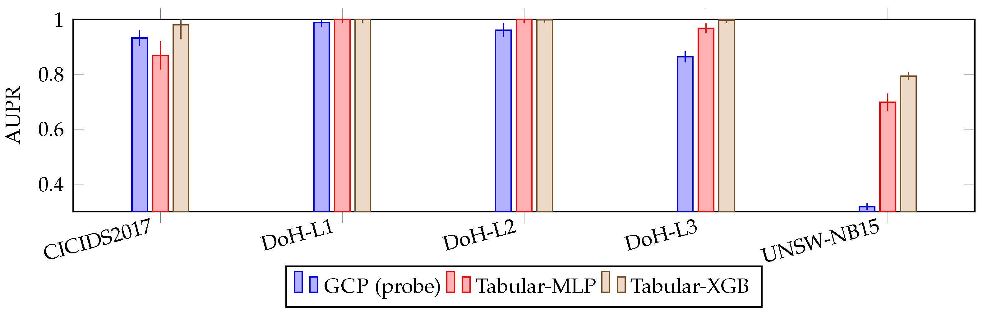
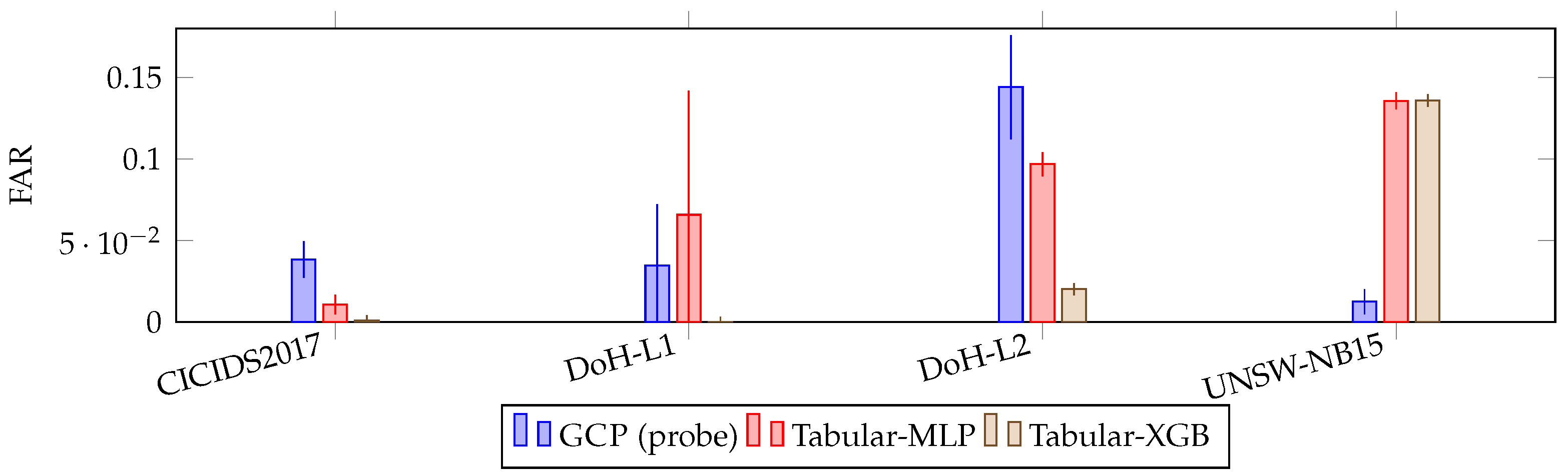
To facilitate readability, we provide comparisons using bar plots for the threshold-independent metrics AUROC and AUPR (Figure 1, Figure 2, Figure 3, Figure 4 and Figure 5 for y, and Figure 2, Figure 3, Figure 4, Figure 5 and Figure 6 for $y_{multi}$).

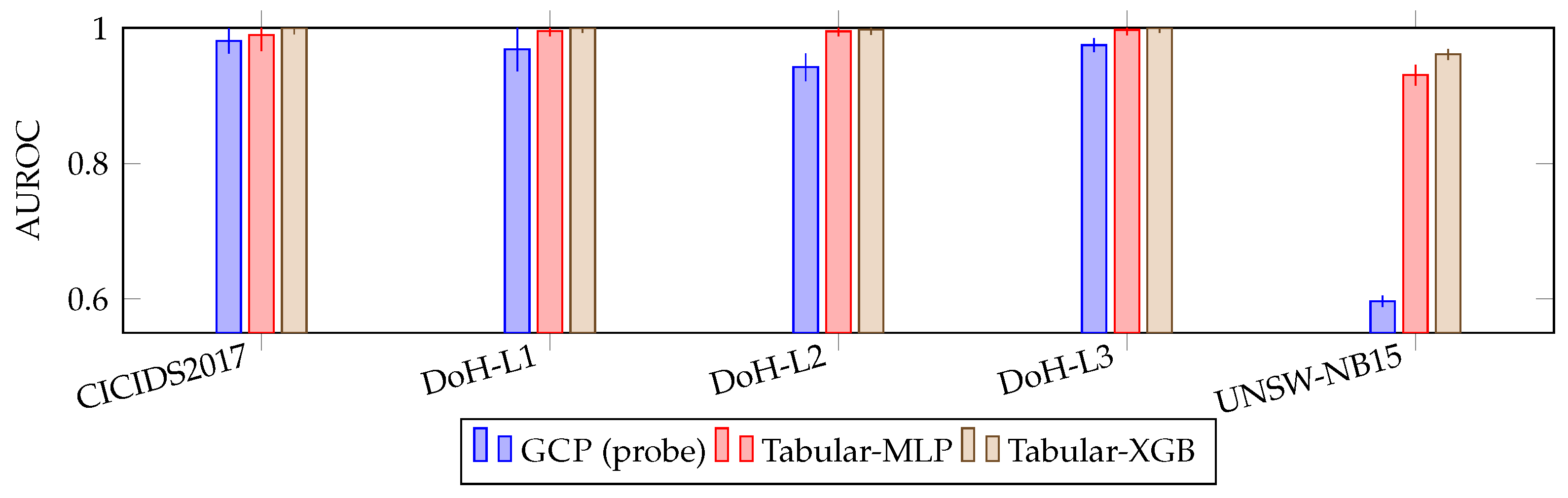
The classification performance for the binary task y is summarized in Figure 1. Tabular-XGB is near-perfect on CICIDS2017 ($\mathrm{AUROC}=0.9990$) and DoH-Combined L1 ($\mathrm{AUROC}=1.0000$), and remains high on DoH-Combined L2 ($\mathrm{AUROC}=0.9973$). The GCP probe is competitive on UNSW-NB15 ($\mathrm{AUROC}=0.9981$) and DoH-Combined L1 ($\mathrm{AUROC}=0.9687$), but drops on DoH-Combined L2 ($\mathrm{AUROC}=0.9412$) (Table 4).

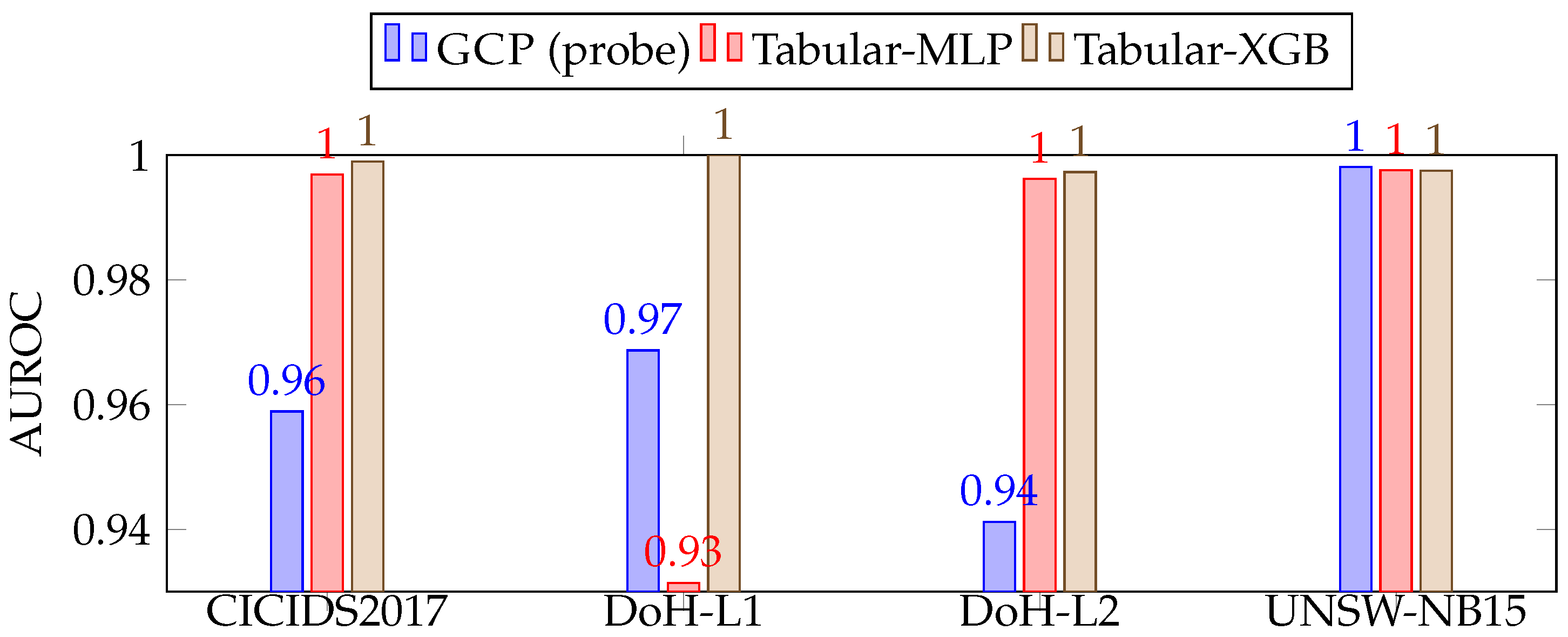
The AUROC performance for $y_{\mathrm{multi}}$ is summarized in Figure 2 (values from Table 5). On CICIDS2017 and the DoH datasets, tabular baselines remain near-ceiling, while the GCP probe is competitive but consistently below XGBoost on DoH-L2 (0.9420 [0.9290, 0.9550] vs. 0.9973 [0.9971, 0.9975]). The most salient deviation occurs on UNSW-NB15, where the probe collapses in AUROC (0.5966 [0.5956, 0.5975]) while tabular baselines remain strong (0.9305–0.9611), anticipating the corresponding macro-F1 degradation reported in Table 5.

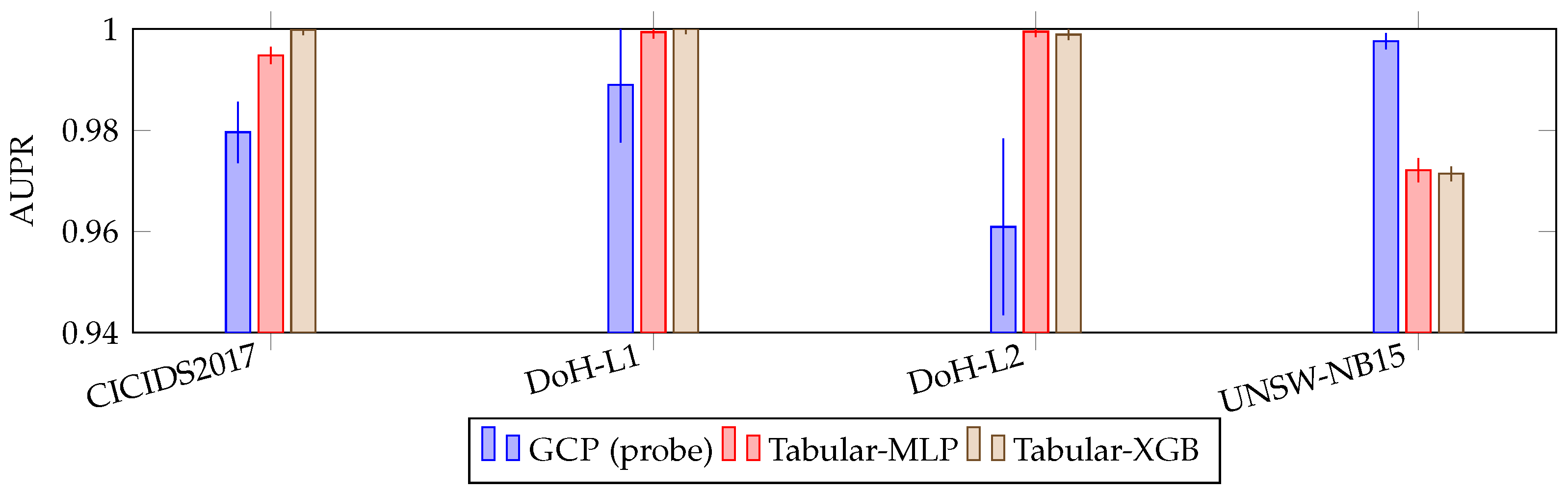
The AUPR results for task y are presented in Figure 3 (values from Table 4). As expected under class imbalance, AUPR complements AUROC by emphasizing early precision at useful recall levels [17,18]. On DoH-L2, the GCP probe shows substantially lower AUPR than tabular baselines (0.9609 [0.9444, 0.9774] vs. MLP 0.9995 [0.9994, 0.9996] and XGB 0.9989 [0.9988, 0.9990]), consistent with the AUROC drop on the same dataset. Conversely, on UNSW-NB15 the probe achieves markedly higher AUPR (0.9976 [0.9970, 0.9982]) than tabular baselines (about 0.971–0.972), indicating improved ranking quality for the positive class in that domain [17,18].

The AUPR performance for $y_{\mathrm{multi}}$ is illustrated in Figure 4 (values from Table 5). On CICIDS2017 and the DoH datasets, tabular baselines remain near-ceiling, while the GCP probe is competitive but lower on DoH-L2 and DoH-L3 (e.g., DoH-L2: 0.9613 [0.9464, 0.9762] vs. XGB 0.9989 [0.9988, 0.9990]). The clearest failure mode occurs on UNSW-NB15, where the probe collapses in AUPR (0.3174 [0.3166, 0.3181]) while tabular baselines remain substantially higher (0.6986–0.7939). This is consistent with the low macro-F1 for the probe in Table 5, indicating poor rare-class recovery rather than a thresholding artifact [17,18].

The operational implications of each method are further elucidated by the FAR results shown in Figure 5 (values from Table 4). On DoH-L2, the GCP probe incurs a markedly higher FAR (0.1440 [0.1150, 0.1730]) than tabular baselines, especially XGBoost (0.0202 [0.0194, 0.0210]), matching the AUROC/AUPR degradation on the same dataset. In contrast, on UNSW-NB15 the probe reduces FAR to 0.0126 [0.0079, 0.0173] while tabular baselines exhibit much higher false-alarm rates (about 0.1356–0.1357), indicating a materially different operating cost despite similarly high AUROC values [2,6].

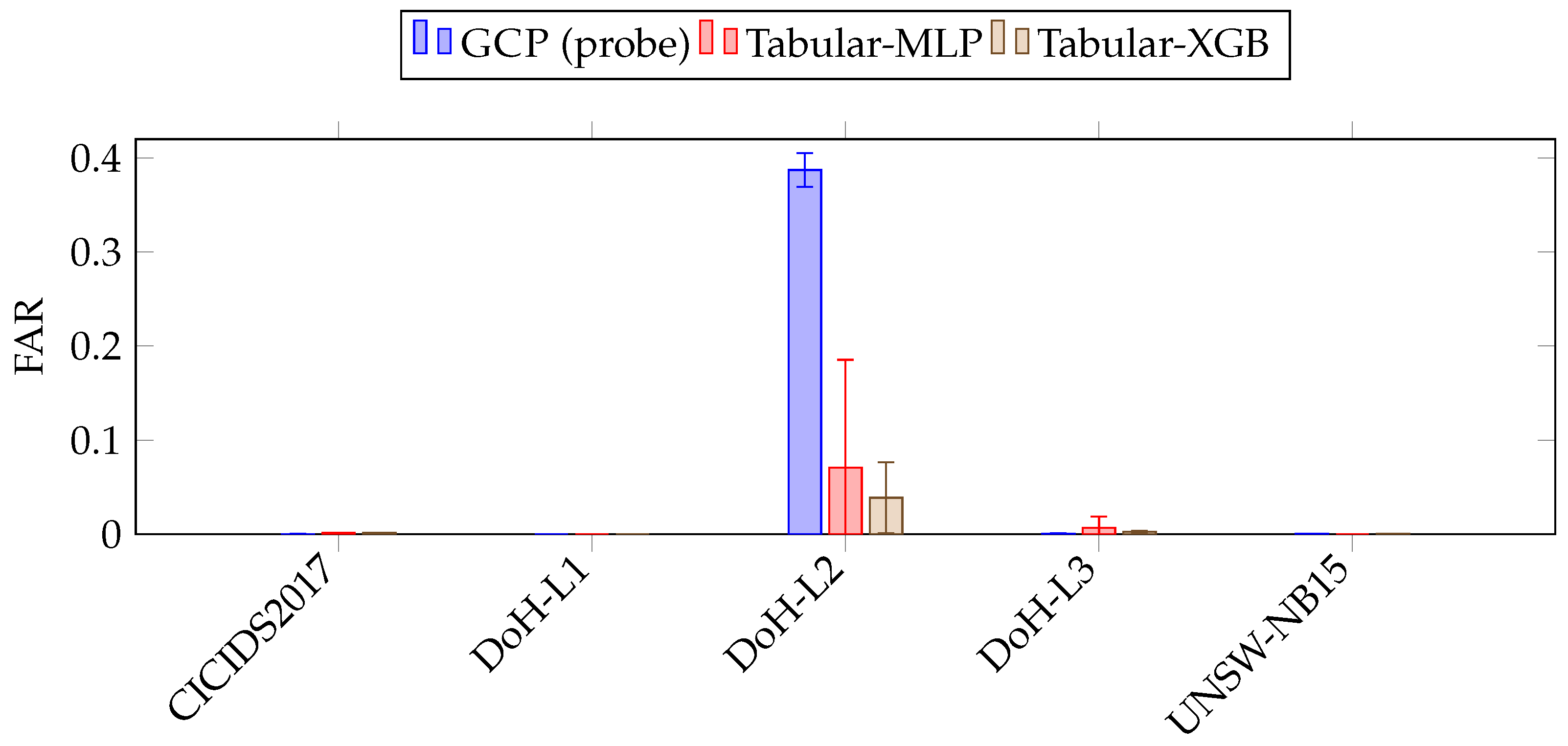
The operational performance in the multiclass task ($y_{\mathrm{multi}}$) is characterized by the FAR results in Figure 6. To enable a single false-alarm notion comparable across datasets [2,6], FAR is computed by collapsing all attack classes into a single “alarm” class (benign vs. non-benign). On CICIDS2017 and DoH-Combined L3, the GCP probe yields the lowest FAR ($0.000166\pm 0.000061$ and $0.000626\pm 0.000215$, respectively), while Tabular-XGB is lowest on DoH-Combined L2 ($0.038677\pm 0.037903$). Notably, for GCP on DoH-Combined L2, the FAR reaches $0.387128\pm 0.017904$ (95% CI, $n=5$ seeds), meaning that roughly $39\%$ of benign flows are incorrectly flagged as attacks. This represents a critical operational cost, as such high false-alarm rates can dominate analyst workload under realistic base rates. Consequently, these results must be interpreted in conjunction with AUROC/AUPR and macro-F1 metrics in Table 5; in particular, UNSW-NB15 shows that a low FAR (e.g., GCP: $0.000381\pm 0.000065$) can coexist with poor macro-F1 when attack classes are missed (low recall), so FAR alone is not sufficient to claim effective multi-class detection.

3.6. Operational Robustness and Error Analysis

To further scrutinize the classification reliability and the impact of class imbalance, we examine the average confusion matrices for both binary and multiclass tasks. This granular analysis allows for a direct inspection of the trade-offs between False Positives (FP) and True Negatives (TN), providing insights into the silent operational regimes and the models’ sensitivity to low-frequency attack samples in specific domains such as UNSW-NB15.

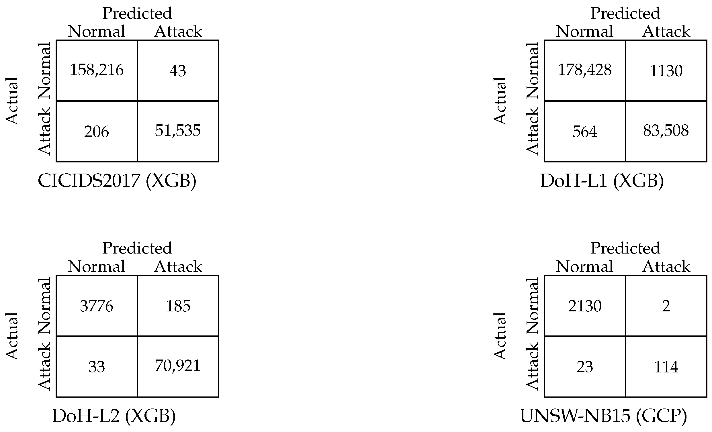
The average confusion matrices, presented in Figure 7, corroborate that for the binary task y, the FAR is predominantly driven by the False Positive (FP) count in scenarios where the True Negative (TN) pool is relatively small. Specifically, for DoH-L2 (XGBoost), we observe $FP=185$ and $TN=3776$ (yielding a $FAR\approx 0.0467$), whereas on UNSW-NB15 (GCP), the metrics improve significantly to $FP=2$ and $TN=2130$ ($FAR\approx 9.4\times {10}^{-4}$). Notably, in CICIDS2017 (XGBoost), the $FP=43$ over $TN\approx 1.58\times {10}^5$ results in a $FAR\approx 2.7\times {10}^{-4}$, reflecting a highly stable operational regime characterized by minimal noise.

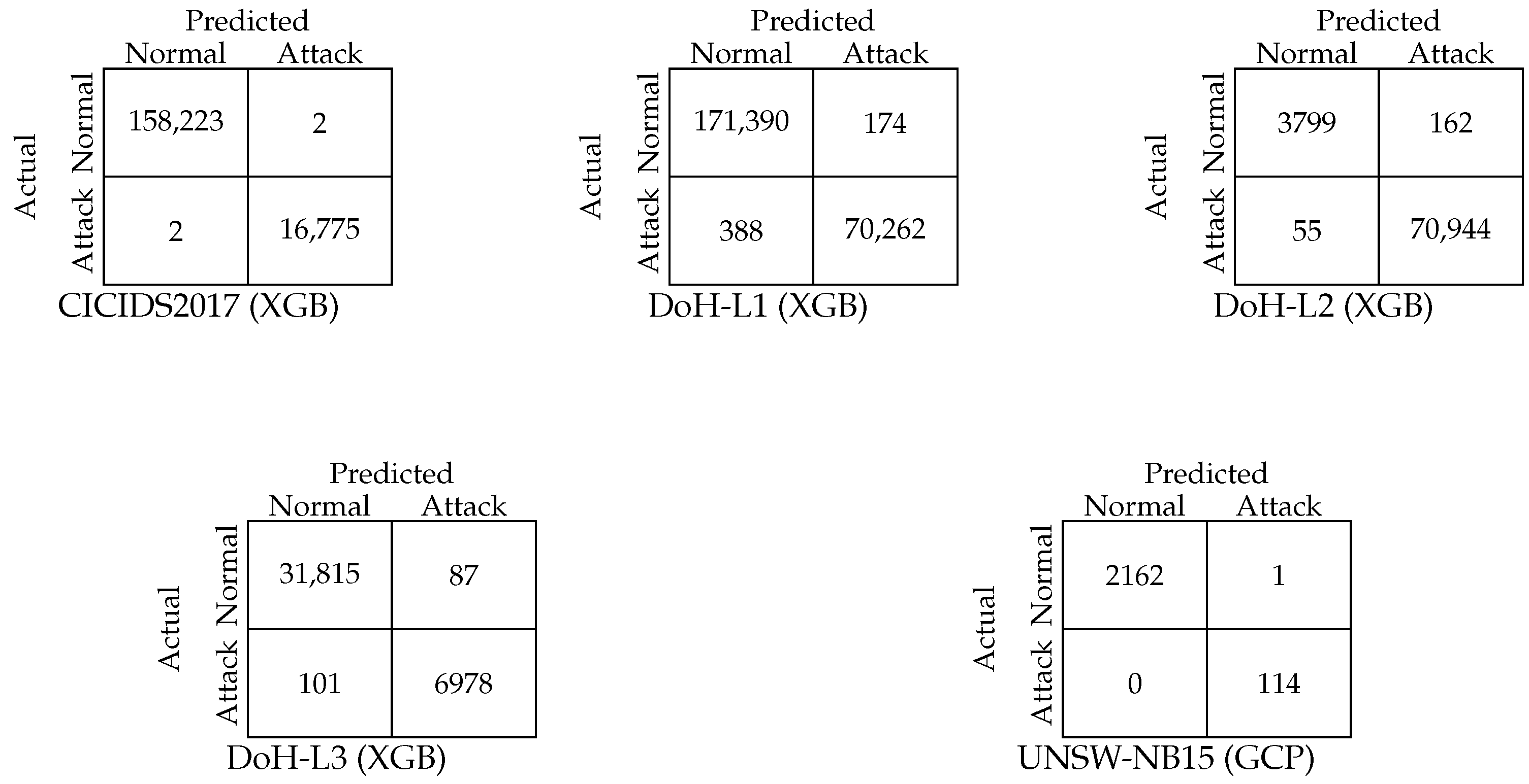
Figure 8 provides an attack-collapsed view (Benign vs. Any-Attack) induced by $y_{\mathrm{multi}}$ predictions. We include it to make class prevalence explicit, which is essential when interpreting FAR and AUPR under skewed base rates [2,6]. For example, in the evaluated split CICIDS2017 contains $TN\approx 158,223$ benign instances versus $TP\approx 16,775$ attacks (XGB), while UNSW-NB15 contains $TN\approx 2162$ benign versus $TP\approx 114$ attacks (GCP). These prevalence differences contextualize (i) the FAR comparisons in Figure 6 and (ii) the ranking-based behavior summarized by AUPR/AUROC in Figure 4 and Table 5.

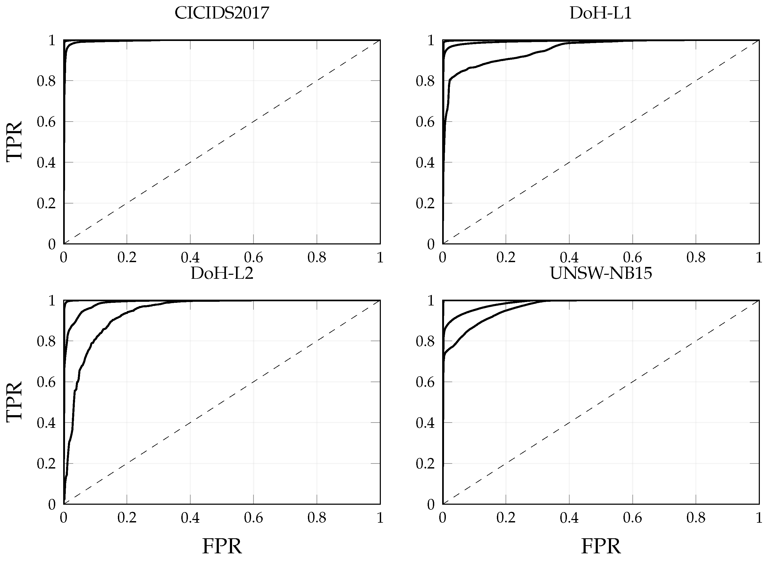
• In-domain ROC behavior (y).

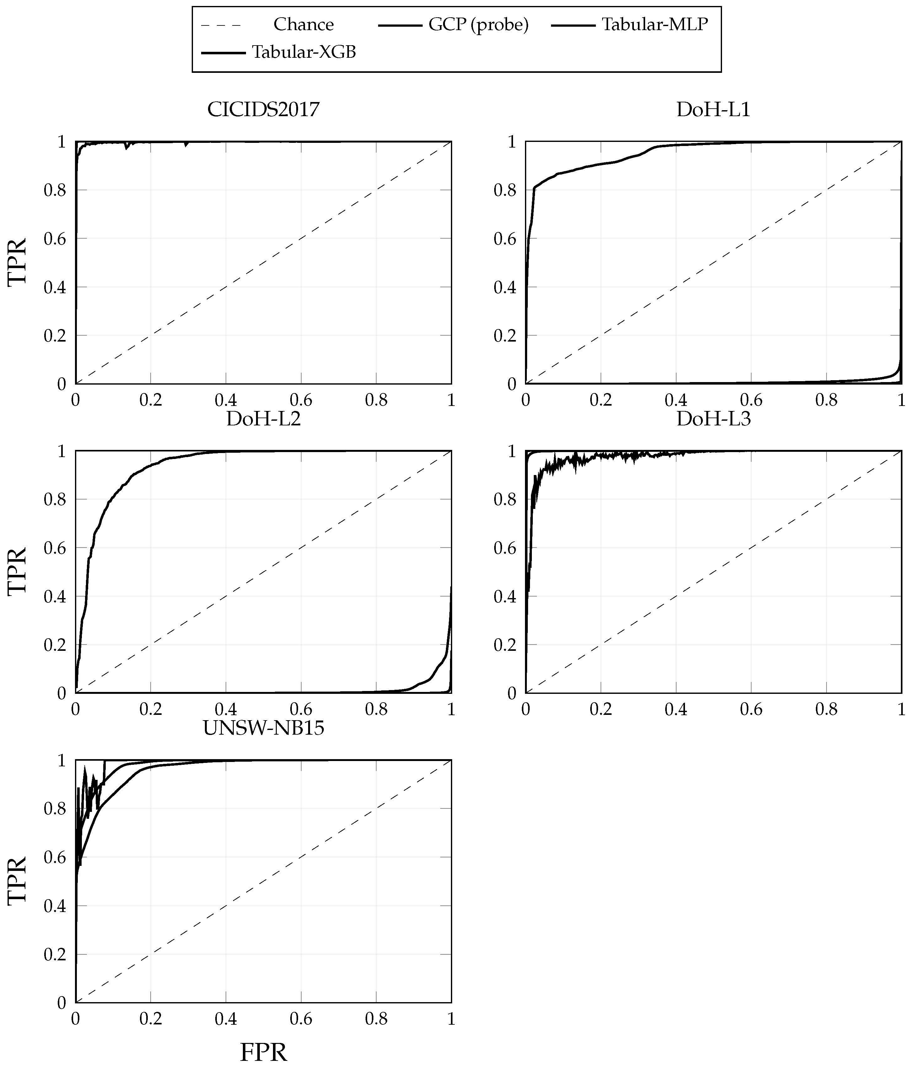
Across datasets, ROC mainly reflects global rank separability. Consistent with Table 4, we expect near-ceiling ROC for feature-separable regimes (e.g., CICIDS2017, DoH-L1/L2) and comparatively weaker ROC for the method/dataset pairs where FAR indicates operational brittleness at low FPR (notably the probe on DoH-L2). Full ROC/PR curves are provided in Figure 9 and Figure 10 (y) and Figure 11 and Figure 12 ($y_{multi}$) [17].

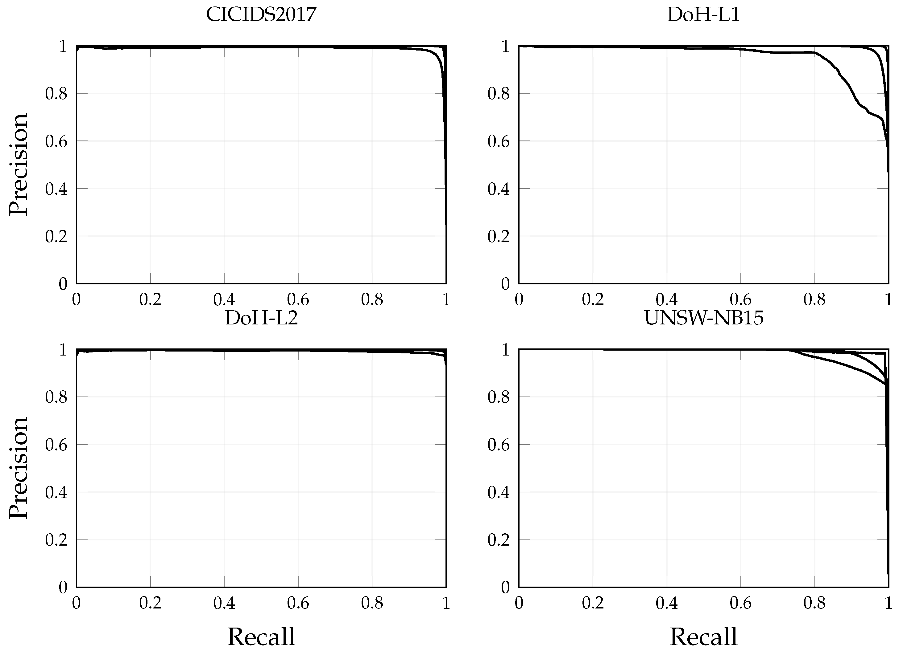
• In-domain PR behavior (y).

PR is more diagnostic under skewed prevalence. When AUROC values are all high, PR and the low-recall/high-precision region can still differentiate methods (e.g., DoH variants). This aligns with the discussion that ROC alone can understate false-alarm costs [18].

• ROC behavior under $y_{\mathrm{multi}}$.

For multi-class/multi-label evaluation, ROC summarizes rank separability under the aggregation used by the pipeline. As indicated in Table 5, some settings can maintain high AUROC while Macro-F1 degrades, which motivates reading ROC jointly with PR and FAR.

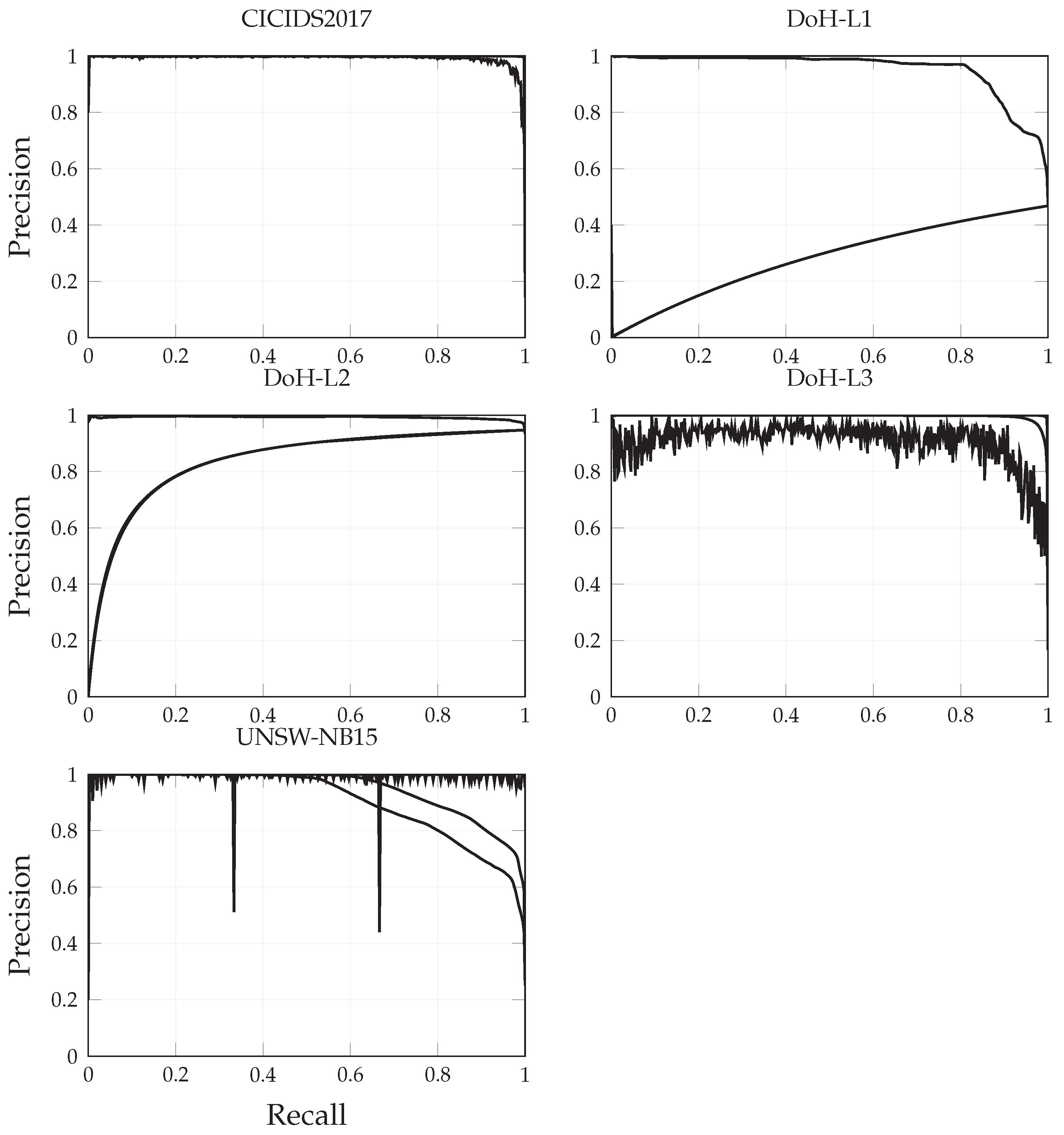
• PR behavior under $y_{\mathrm{multi}}$ and rare-class effects.

PR is sensitive to rare-class recovery. The UNSW-NB15 multi-class setting is expected to show markedly weaker PR for tabular baselines relative to the probe (consistent with the sharp AUPR gap discussed around Figure 4), while DoH-family datasets remain near-ceiling due to strong feature-driven separability.

4. Conclusions and Future Works

We introduced GCP, a payload-free graph-contrastive pretraining framework for encrypted-traffic intrusion detection, and evaluated it with a fully scripted pipeline that freezes run manifests and intermediate artifacts so that every reported number is traceable to a concrete run directory.

Across CICIDS2017, UNSW-NB15, and DoH-Combined (L1/L2/L3), and for both y and $y_{\mathrm{multi}}$, the results support three main conclusions. First, GCP delivers its clearest in-domain benefit on UNSW-NB15 for binary detection, achieving near-ceiling Macro-F1 while substantially reducing FAR compared with strong tabular baselines. Second, in feature-separable regimes (CICIDS2017 and DoH-L1/L2), boosted trees remain difficult to surpass, and our ablations show that graph structure alone does not provide consistent gains without the contrastive pretraining signal. Third, OOD transfer is strongly source–target dependent: transfer is most reliable within closely related DoH domains, while cross-family transfer can degrade sharply under dataset shift.

Future work will focus on (i) scaling pretraining (more epochs and larger graphs) and extending augmentations to better preserve task-relevant invariances, (ii) improving robustness under distribution shift via explicit domain-adaptation or calibration strategies, and (iii) expanding evaluation to additional encrypted-traffic benchmarks and deployment-motivated operating points.

References

1. Hoffman, P.; McManus, P. DNS Queries over HTTPS (DoH); IETF RFC 8484; IETF: Fremont, CA, USA, 2018. [Google Scholar]
2. Axelsson, S. The Base-Rate Fallacy and the Difficulty of Intrusion Detection. ACM Trans. Inf. Syst. Secur. 2000, 3, 186–205. [Google Scholar] [CrossRef]
3. Chen, T.; Guestrin, C. XGBoost: A Scalable Tree Boosting System. In Proceedings of the 22nd ACM SIGKDD International Conference on Knowledge Discovery and Data Mining (KDD), San Francisco, CA, USA, 13–17 August 2016; pp. 785–794. [Google Scholar]
4. Buczak, A.L.; Guven, E. A Survey of Data Mining and Machine Learning Methods for Cyber Security Intrusion Detection. IEEE Commun. Surv. Tutor. 2016, 18, 1153–1176. [Google Scholar] [CrossRef]
5. Quionero-Candela, J.; Sugiyama, M.; Schwaighofer, A.; Lawrence, N.D. Dataset Shift in Machine Learning; MIT Press: Cambridge, MA, USA, 2008. [Google Scholar]
6. Sommer, R.; Paxson, V. Outside the Closed World: On Using Machine Learning for Network Intrusion Detection. In Proceedings of the IEEE Symposium on Security and Privacy (S&P), Oakland, CA, USA, 16–19 May 2010; pp. 305–316. [Google Scholar]
7. Liu, X.-M.; Chang, X.-H.; Hou, L.-W. Attack-Dependent Adaptive Event-Triggered Security Fuzzy Control for Nonlinear Networked Cascade Control Systems Under Deception Attacks. Mathematics 2024, 12, 3385. [Google Scholar] [CrossRef]
8. Liu, X.-M.; Chang, X.-H. Adaptive event-triggered tracking control for nonlinear networked systems with dynamic quantization and deception attacks. Int. J. Robust Nonlinear Control 2024, 34, 8311–8333. [Google Scholar] [CrossRef]
9. Arcos-Argudo, M.; Bojorque, R.; Torres, A. A Deterministic Comparison of Classical Machine Learning and Hybrid Deep Representation Models for Intrusion Detection on NSL-KDD and CICIDS2017. Algorithms 2025, 18, 749. [Google Scholar] [CrossRef]
10. van den Oord, A.; Li, Y.; Vinyals, O. Representation Learning with Contrastive Predictive Coding. arXiv 2018, arXiv:1807.03748. [Google Scholar]
11. Chen, T.; Kornblith, S.; Norouzi, M.; Hinton, G. A Simple Framework for Contrastive Learning of Visual Representations. In Proceedings of the 37th International Conference on Machine Learning (ICML), Virtual, 13–18 July 2020; pp. 1597–1607. [Google Scholar]
12. Velićkovixcx, P.; Fedus, W.; Hamilton, W.L.; Liò, P.; Bengio, Y.; Hjelm, R.D. Deep Graph Infomax. In Proceedings of the 7th International Conference on Learning Representations (ICLR), New Orleans, LA, USA, 6–9 May 2019. [Google Scholar]
13. You, Y.; Chen, T.; Sui, Y.; Chen, T.; Wang, Z.; Shen, Y. Graph Contrastive Learning with Augmentations. In Proceedings of the 34th Annual Conference on Neural Information Processing Systems (NeurIPS), Virtual, 6–12 December 2020. [Google Scholar]
14. Sharafaldin, I.; Lashkari, A.H.; Ghorbani, A.A. Toward Generating a New Intrusion Detection Dataset and Intrusion Traffic Characterization. In Proceedings of the 4th International Conference on Information Systems Security and Privacy (ICISSP), Madeira, Portugal, 22–24 January 2018; pp. 108–116. [Google Scholar]
15. Moustafa, N.; Slay, J. UNSW-NB15: A Comprehensive Data Set for Network Intrusion Detection Systems (UNSW-NB15 Network Data Set). In Proceedings of the IEEE Military Communications Conference (MILCOM), Tampa, FL, USA, 26–28 October 2015; pp. 1–6. [Google Scholar]
16. MontazeriShatoori, M.; Golestan, L.; Hamadi, E.A.; Lashkari, A.H.; Ghorbani, A.A. Detection of DoH Tunnels Using Time-Series Classification of Encrypted Traffic. In Proceedings of the IEEE International Conference on Communications (ICC), Dublin, Ireland, 7–11 June 2020; pp. 1–6. [Google Scholar]
17. Davis, J.; Goadrich, M. The Relationship Between Precision-Recall and ROC Curves. In Proceedings of the 23rd International Conference on Machine Learning (ICML), Pittsburgh, PA, USA, 25–29 June 2006; pp. 233–240. [Google Scholar]
18. Saito, T.; Rehmsmeier, M. The Precision-Recall Plot is More Informative than the ROC Plot When Evaluating Binary Classifiers on Imbalanced Datasets. PLoS ONE 2015, 10, e0118432. [Google Scholar] [CrossRef] [PubMed]
19. Kipf, T.N.; Welling, M. Semi-Supervised Classification with Graph Convolutional Networks. In Proceedings of the 5th International Conference on Learning Representations (ICLR), Toulon, France, 24–26 April 2017. [Google Scholar]
20. Velićkovixcx, P.; Cucurull, G.; Casanova, A.; Romero, A.; Liò, P.; Bengio, Y. Graph Attention Networks. In Proceedings of the 6th International Conference on Learning Representations (ICLR), Vancouver, BC, Canada, 30 April–3 May 2018. [Google Scholar]
21. Hamilton, W.L. Graph Representation Learning; Morgan & Claypool Publishers: San Rafael, CA, USA, 2020. [Google Scholar]
22. Wasserman, L. All of Statistics: A Concise Course in Statistical Inference; Springer: Berlin/Heidelberg, Germany, 2004. [Google Scholar]
23. Paszke, A.; Gross, S.; Massa, F.; Lerer, A.; Bradbury, J.; Chanan, G.; Killeen, T.; Lin, Z.; Gimelshein, N.; Antiga, L.; et al. PyTorch: An Imperative Style, High-Performance Deep Learning Library. In Proceedings of the NeurIPS, Vancouver, BC, Canada, 8–14 December 2019; pp. 8024–8035. [Google Scholar]
24. Fey, M.; Lenssen, J.E. Fast Graph Representation Learning with PyTorch Geometric. In Proceedings of the ICLR Workshop on Representation Learning on Graphs and Manifolds, New Orleans, LA, USA, 6–9 May 2019. [Google Scholar]
25. Pedregosa, F.; Varoquaux, G.; Gramfort, A.; Michel, V.; Thirion, B.; Grisel, O.; Blondel, M.; Prettenhofer, P.; Weiss, R.; Dubourg, V.; et al. Scikit-learn: Machine Learning in Python. J. Mach. Learn. Res. 2011, 12, 2825–2830. [Google Scholar]
26. Harris, C.R.; Millman, K.J.; van der Walt, S.J.; Gommers, R.; Virtanen, P.; Cournapeau, D.; Wieser, E.; Taylor, J.; Berg, S.; Smith, N.J.; et al. Array Programming with NumPy. Nature 2020, 585, 357–362. [Google Scholar] [CrossRef] [PubMed]
27. McKinney, W. Data Structures for Statistical Computing in Python. In Proceedings of the Python in Science Conference (SciPy), Austin, TX, USA, 28 June–3 July 2010; pp. 56–61. [Google Scholar]
28. Canadian Institute for Cybersecurity. CICIDS2017 Dataset. University of New Brunswick, 2017. Available online: https://www.unb.ca/cic/datasets/ids-2017.html (accessed on 5 February 2025).
29. UNSW Canberra Cyber. The UNSW-NB15 Dataset, 2015. Available online: https://research.unsw.edu.au/projects/unsw-nb15-dataset (accessed on 6 March 2026).
30. Canadian Institute for Cybersecurity. CIRA-CIC-DoHBrw-2020 Dataset. 2020. Available online: https://www.unb.ca/cic/datasets/dohbrw-2020.html (accessed on 6 March 2026).
Figure 1. In-domain AUROC for y on four datasets. Error bars: 95% confidence intervals over 5 seeds. Values match those shown in Table 4.
Algorithms 19 00389 g001
Figure 2. In-domain AUROC for y multi across datasets. Error bars show 95% CI across seeds. Values match those shown in Table 5.
Algorithms 19 00389 g002
Figure 3. In-domain AUPR for y across datasets. Error bars show 95% CI across seeds. Values match those shown in Table 4.
Algorithms 19 00389 g003
Figure 4. In-domain AUPR for y multi across datasets. Error bars show 95% CI across seeds. Values match those shown in Table 5.
Algorithms 19 00389 g004
Figure 5. In-domain False Alarm Rate (FAR) for y. Error bars show 95% CI across seeds. Values match those shown in Table 4.
Algorithms 19 00389 g005
Figure 6. In-domain FAR for y multi (benign vs. non-benign collapse). Error bars show 95% confidence intervals over 5 seeds.
Algorithms 19 00389 g006
Figure 7. Average confusion matrices (rounded) over 5 seeds for the binary task y (Normal vs. Attack). We show Tabular-XGB for CICIDS2017/DoH-Combined L2/DoH-Combined L3 and GCP (probe) for UNSW-NB15 (best AUPR in that case).
Algorithms 19 00389 g007
Figure 8. Attack-collapsed (Benign vs. Any-Attack) confusion matrices induced by multiclass predictions y multi : all non-benign classes are merged into a single Attack label. Entries are mean counts over 5 seeds (rounded). To keep the figure compact, we show one representative method per dataset (XGB for CICIDS2017/DoH and GCP for UNSW-NB15); quantitative FAR comparisons across methods are reported in Figure 6.
Algorithms 19 00389 g008
Figure 9. ROC curves (mean across seeds; optional 95% band if available) for y on each dataset. Curves are computed from the same prediction scores used to report AUROC/AUPR in the tables.
Algorithms 19 00389 g009
Figure 10. Precision–Recall (PR) curves (mean across seeds; optional 95% band if available) for y on each dataset. Curves are computed from the same prediction scores used to report AUROC/AUPR in the tables.
Algorithms 19 00389 g010
Figure 11. ROC curves (mean across seeds; optional 95% band if available) for y multi on each dataset. Curves are computed from the same prediction scores used to report AUROC/AUPR in the tables.
Algorithms 19 00389 g011
Figure 12. Precision–Recall (PR) curves (mean across seeds; optional 95% band if available) for y multi on each dataset. Curves are computed from the same prediction scores used to report AUROC/AUPR in the tables.
Algorithms 19 00389 g012