Genetic Programming Algorithm Evolving Robust Unary Costs for Efficient Graph Cut Segmentation

Abstract

Accurate cell and nuclei segmentation remains challenging due to the sensitivity of classical graph-cut methods to parameter tuning. While deep learning models like U-Net offer strong performance, they require large annotated datasets and substantial GPU resources. This work presents a cost-effective alternative: a genetic programming (GP) framework that jointly optimizes unary cost functions and regularization parameters for graph-cut segmentation, coupled with automatic seed selection. Evaluation is conducted under two distinct protocols: (1) oracle-guided per-image optimization, establishing upper-bound performance (mean Dice 0.822, IoU 0.733), and (2) true generalization via train/test split, where expressions learned on 50 images are applied to 50 unseen images (mean Dice 0.695, IoU 0.588). The fixed-model generalization still significantly outperforms the baseline graph cut ($+0.158$ Dice, $p<0.001$). Cross-dataset validation on MoNuSeg (H&E histopathology) achieves a Dice score of 0.823 with the fixed GP model, significantly outperforming the baseline (+0.272). This result uses a single fixed model—the best-performing expression from BBBC038 training—applied in a zero-shot manner to MoNuSeg without any retraining or domain adaptation. All 100 images showed non-negative improvement under oracle optimization in the experiments. The method requires no GPU training, runs in 550 s per image for oracle search, and offers interpretable symbolic cost functions. Code and annotations are provided to ensure reproducibility. This approach offers a practical, interpretable alternative in resource-constrained biomedical imaging settings.

1. Introduction

Segmenting individual cells and nuclei in microscopy images is a fundamental step in many biological and clinical pipelines, including phenotyping, drug screening, and digital pathology. Errors at the segmentation stage directly propagate to downstream measurements such as cell counts, morphological statistics, and intensity-based biomarkers. Despite substantial progress in deep learning for biomedical image segmentation, classical energy-minimization methods such as graph cuts remain appealing because they provide globally optimal solutions for binary labeling problems under certain conditions and can be implemented efficiently on CPUs.

In the conventional source–sink graph-cut formulation, segmentation quality depends strongly on two design aspects: the unary data terms, which encode the cost of assigning each pixel to the foreground or background, and the pairwise regularization terms, which control boundary smoothness and contrast sensitivity. Both are typically hand-crafted from intensity and gradient information and require user-chosen parameters such as $\gamma$ (data weight), $\lambda$ (smoothness weight), and $\beta$ (edge contrast scaling). Furthermore, interactive graph-cut tools rely on user-provided scribbles or seeds, making the results sensitive to human input.

At the other end of the spectrum, deep convolutional architectures such as U-Net and nnU-Net are now the established standard for biomedical segmentation. They can learn rich features and shape priors directly from data, but at the cost of intensive GPU training, careful data augmentation, and non-trivial deployment complexity. Previous research has demonstrated that high segmentation quality can be obtained with carefully designed training schedules and limited GPU budgets for deep learning models [1]. This study investigates whether competitive segmentation performance can be attained while preserving the lightweight and interpretable nature of the graph-cut paradigm, without aiming to replace deep learning approaches in data-rich settings.

The full methodology—including the seed-selection strategy, genetic program representation, unary cost modulation, and optimization pipeline—is detailed in Section 3.

Contributions

The main contributions of this work are:

1. A genetic programming framework that jointly optimizes graph-cut regularization parameters and symbolic unary cost functions. this framework was explicitly evaluated under two protocols: (a) oracle-guided per-image optimization (using ground truth for fitness) to establish upper-bound performance (Dice 0.822), and (b) true generalization via a train/test split, where expressions learned on 50 images are applied to 50 unseen images (Dice 0.695, +0.158 over baseline).

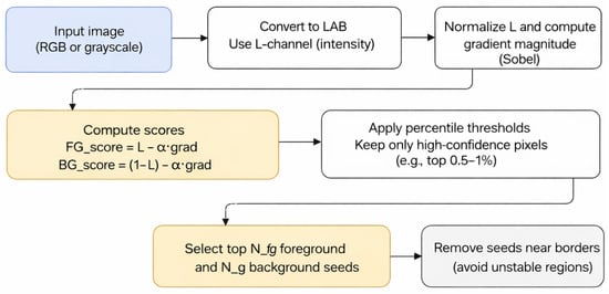
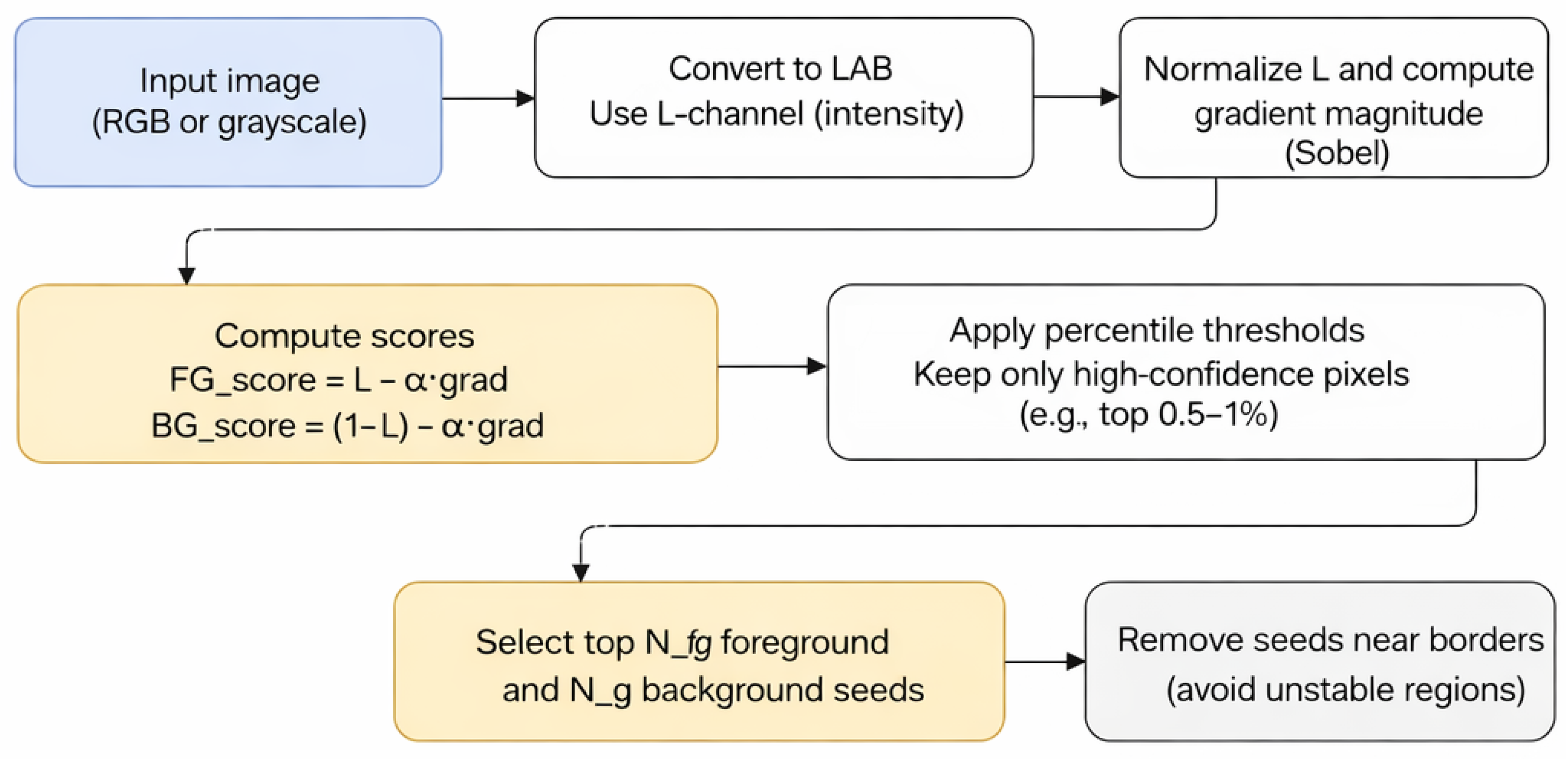
2. An automatic seed-selection strategy that identifies high-confidence foreground and background pixels using a simple, interpretable scoring function in Lab color space, as visualized in Figure 1. This strategy eliminates manual annotation while maintaining robustness across diverse image conditions.

Figure 1. Automatic seed selection pipeline.

3. A multi-faceted evaluation, including oracle upper bounds, true generalization, cross-dataset transfer (MoNuSeg Dice 0.823 with a fixed GP model, $+0.272$ over baseline), and ablation studies, isolating the contributions of seed selection, parameter tuning, and symbolic structure.

4. Interpretable cost functions, with multiple representative evolved expressions analyzed, demonstrating consistent biological patterns (bright, smooth nuclei; dark, smooth background) rather than overfitted artifacts.

5. Open science practices, with code, per-image CSV results, and seed annotations provided for reproducibility.

2. Related Work

2.1. Graph Cuts for Image Segmentation

Graph-cut methods [2,3,4] have been widely used for interactive image segmentation, where users mark foreground and background regions, and a source/sink min-cut yields the globally optimal binary labeling under an energy of the form.

$$E\left(L\right)=\sum _p{D}_p\left(L_p\right)+\lambda \sum _{(p,q)\in \mathcal{N}}{V}_{p,q}\mathbb{I}[L_p\ne L_q],$$

(1)

where $L_p\in \{\mathrm{FG},\mathrm{BG}\}$ is the label of pixel p, $D_p$ are unary data costs, and $V_{p,q}$ are pairwise terms over a neighborhood $\mathcal{N}$. Variants differ in how these terms are constructed from intensity models, (e.g., GMMs) and edge weights based on gradients or color differences. Recent advancements in graph-cut segmentation have explored combining graph cuts with richer appearance or shape information in medical imaging. For instance, Chen et al. [5] combined graph cuts with oriented active appearance models to improve robustness in medical image segmentation. More recently, Chen et al. [6] proposed a modified graph-cut segmentation method with adaptive shape constraints and demonstrated its effectiveness on computed tomography images. These works highlight the ongoing relevance of graph-cut formulations when enhanced with domain-specific priors.

2.2. Evolutionary Optimization in Computer Vision

Evolutionary algorithms, including genetic algorithms and genetic programming, have been applied to feature selection, model parameter tuning, and symbolic regression in computer vision. GP is particularly attractive when the functional form of the desired mapping is unknown and interpretability is desirable, as it evolves tree-based expressions from a primitive set of arithmetic operators and functions. Applications to segmentation have typically focused on evolving pixel-wise classifiers or edge detectors, or on tuning parameters of existing methods. However, relatively few works directly target graph-cut unary cost design and global parameter tuning for medical image segmentation. Foundational work in genetic programming includes the field guide by Poli et al. [7] and early GP applications to system identification by Iba et al. [8], which established GP as a practical framework for discovering interpretable symbolic models. Moreover, Mabrouk et al. [9] proposed an immune system programming approach for medical image segmentation, demonstrating the versatility of bio-inspired evolutionary algorithms in biomedical applications. Multi-objective optimization and evolutionary strategies have also been discussed as practical tools for balancing segmentation accuracy and computational cost; a comprehensive overview is provided by Mittal et al. [10]. These contemporary approaches underscore the growing potential of evolutionary methods in addressing complex segmentation challenges.

Classical evolutionary approaches to image segmentation include the work of Bhandarkar and Zhang [11], which provides an early, well-cited foundation for evolutionary computation in segmentation. Nosrati and Hamarneh [12] explored evolutionary computation for cell segmentation under partial occlusion and configuration constraints, highlighting the relevance of evolutionary strategies in challenging microscopy conditions. The proposed work differs in multiple aspects. First, it jointly optimizes both unary cost functions and regularization parameters within a unified GP framework. Second, it integrates automatic seed selection to eliminate manual intervention. Finally, it specifically targets challenging biomedical segmentation scenarios with overlapping nuclei, where traditional graph cuts struggle.

2.3. Automatic Seed Selection and Cell Segmentation

Automatic seed generation has been explored in watershed-based and multi-label segmentation, often using distance transforms, regional maxima, or superpixels to initialize markers. In the context of binary graph cuts, automatically derived seeds can reduce user dependency and enable per-image optimization. For cell and nuclei segmentation, a large body of work is based on U-Net-like architectures, with nnU-Net providing strong out-of-the-box performance at the cost of substantial training resources. The proposed method is complementary: it focuses on binary nuclei/background segmentation with minimal supervision and computation, while still leveraging global optimization via graph cuts. Recent innovations in reducing annotation and initialization effort include weakly supervised and point-based strategies. Bearman et al. [13] demonstrated effective supervision using sparse point annotations, while Can et al. [14] demonstrated medical image segmentation using scribble supervision, and Kervadec et al. [15] proposed constrained loss formulations for weakly supervised segmentation. These approaches highlight the growing interest in minimizing manual annotation while maintaining segmentation accuracy.

Recent evolutionary segmentation research includes work on geometric energies and active contours [16], and the evolutionary design of morphological operators for microscopy segmentation [17].

The proposed work differs by combining automatic seed selection, GP-evolved unary functions, and joint parameter optimization within a unified pipeline.

3. Materials and Methods

3.1. Genetic Programming for Graph-Cut Optimization

The proposed algorithm integrates genetic programming with graph-cut energy minimization to jointly optimize both the regularization parameters $(\gamma ,\lambda ,\beta )$ and symbolic expressions for unary cost functions. Algorithm 1 outlines the complete optimization procedure.

Algorithm 1 Genetic Programming for Graph-Cut Optimization

Require: Input image I, ground truth mask Y (for fitness only), population size N, and number of generations G

Ensure: Optimized parameters $(\gamma ,\lambda ,\beta )$ and symbolic expressions ${\mathcal{T}}_{\mathrm{FG}},{\mathcal{T}}_{\mathrm{BG}}$

1: Initialize the population with random parameters and expression trees (ramped half-and-half)

2: for $g=1$ to G do

3:    for each individual i in the population do

4:       Compute feature maps: $I,G,D_{\mathrm{FG}},D_{\mathrm{BG}},M,S,C^{\mathrm{FG}},C^{\mathrm{BG}}$

5:       Build modulation maps $a_{\mathrm{FG}},a_{\mathrm{BG}}$ via ${\mathcal{T}}_{\mathrm{FG}},{\mathcal{T}}_{\mathrm{BG}}$ (Equations (8) and (9))

6:       Compute unary costs $D_p^{\mathrm{FG}},D_p^{\mathrm{BG}}$ (Equation (10))

7:       Construct the graph with pairwise weights $V_{p,q}$ (Equation (6))

8:       Run max-flow/min-cut to obtain segmentation $\widehat{Y}$

9:       Compute fitness $f\left(i\right)=\mathrm{Dice}(\widehat{Y},Y)$

10:    end for

11:    Select parents via tournament selection ($k=3$)

12:    Apply one-point crossover (probability 0.8)

13:    Apply mutation: subtree replacement (0.2) and Gaussian jitter on scalars

14:    Preserve the best individual (elitism)

15: end for

16: return Best individual from the final generation

3.2. Dataset

3.2.1. Primary Dataset (BBBC038)

The primary experiments were conducted on a subset of 100 fluorescence microscopy images from the publicly available “2018 Data Science Bowl” dataset [18] (BBBC038), each paired with expert-provided binary nuclei masks. These images span diverse nuclear sizes, contrasts, and clustering patterns. Two evaluation regimes were used on BBBC038: (i) oracle-guided per-image optimization (ground truth used only for fitness on the same image), and (ii) train/test generalization, where GP is optimized on a training subset and then frozen and applied to held-out test images without test-label access. Ground-truth masks are used only for per-image fitness evaluation during optimization; no single global model is trained in the traditional supervised learning sense.

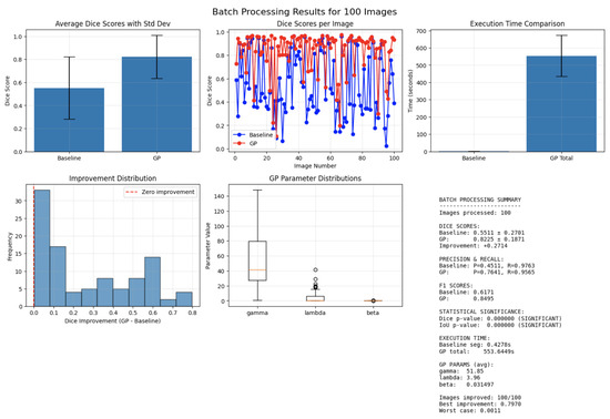
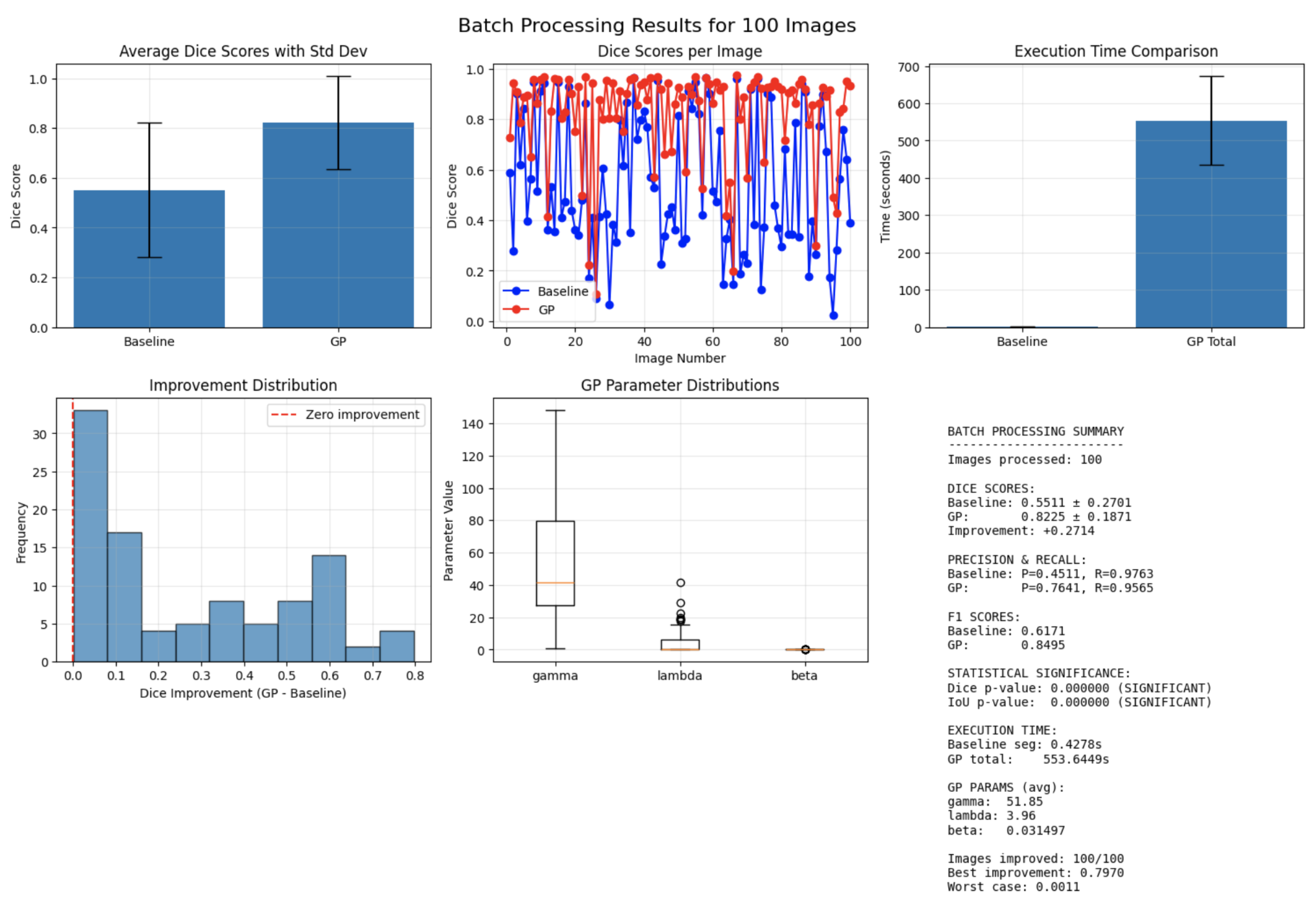
Figure 2 presents the primary dataset analysis. The top row (left) shows the mean Dice scores with standard deviation for the baseline graph cut and the GP-optimized model. The top row (middle) represents the per-image Dice curves, demonstrating consistent GP outperformance across the dataset. The top row (right) shows the execution-time comparison between baseline segmentation and total GP processing.

Figure 2. Batch-processing results for 100 validation images.

The bottom row (left) shows the histogram of Dice improvements (GP − baseline), confirming non-negative gains for all 100 images. The bottom row (middle) presents the GP parameter distributions for $\gamma$, $\lambda$, and $\beta$ across the batch. The bottom row (right) provides a textual summary including mean Dice, precision/recall, F1-scores, execution-time statistics, improvement count (100/100), parameter means, and Wilcoxon significance tests ($p<{10}^{-5}$). The figure underscores robust improvements delivered by GP-optimized graph cuts across all metrics.

Because GP operates on a per-image basis, it can independently optimize each of the 100 BBBC038 images under the oracle setting, eliminating the need for a train/validation split in that specific protocol. Figure 2 visualizes the resulting performance, showing both the distribution of Dice scores and the per-image gains achieved by the evolved unary cost functions.

3.2.2. Secondary Dataset (MoNuSeg)

The MoNuSeg histopathology dataset is used for cross-dataset evaluation. It contains H&E-stained tissue images with markedly different texture and color characteristics. The exact same GP-evolved parameters and unary functions were applied without retraining or domain-specific adjustments. Detailed performance results for this dataset are presented in the next section.

The strong cross-dataset performance on MoNuSeg, despite no retraining, can be attributed to the modality-invariant nature of the feature set and the fact that GP optimizes symbolic cost functions rather than learning texture-specific filters, reducing the risk of overfitting to fluorescence-specific patterns. The intensity, gradient, distance-to-seeds, and local-statistics features capture structural and morphological information that remains stable across fluorescence and H&E modalities. Additionally, because the GP framework optimizes unary costs using symbolic expressions rather than learned convolutional filters, it avoids overfitting to texture or stain-specific patterns, contributing to the method’s robustness under domain shift.

Importantly, both datasets were used exclusively for evaluation and test-time optimization; the proposed method requires no supervised learning, and all improvements arise from GP-evolved cost functions applied independently to each test image.

3.3. Automatic Seed Selection

Foreground and background seeds were selected using a percentile-based criterion. Let $I\left(x\right)$ be the normalized intensity and $G\left(x\right)$ the Sobel gradient magnitude at pixel x. The selection criteria are defined as $s_{\mathrm{FG}}=I-0.6G,s_{\mathrm{BG}}=(1-I)-0.6G.$

Candidate seeds are restricted to an inner region excluding a 10-pixel border. Thresholds ${\tau }_{\mathrm{FG}}$ and ${\tau }_{\mathrm{BG}}$ are set to the 99.5th percentile of $s_{\mathrm{FG}}$ and $s_{\mathrm{BG}}$, and the process retains at most five FG and eight BG seed points per image. These values were selected empirically through stability tests across the 100-image dataset. Multiple configurations ($N_{\mathrm{FG}},N_{\mathrm{BG}}$∈ 3–15) were evaluated and found that larger seed sets (≥15 points) often introduced seeds near ambiguous boundaries, destabilizing the unary terms, whereas very small sets (<3 points) produced incomplete coverage of nuclei regions. The values $N_{\mathrm{FG}}=5$ and $N_{\mathrm{BG}}=8$ consistently yielded the most stable Dice performance (with less than $2.7\%$ relative variation under seed perturbation) while preserving sparsity and interpretability. These values were fixed across all experiments and datasets; no dataset-specific tuning was performed. Given an input image I (RGB or grayscale), it is first converted to Lab color space, and the L-channel is used as intensity. The Lab color space was selected because its L–channel is perceptually uniform and decoupled from chromatic information, making it more robust to illumination changes than raw RGB intensity. Empirically, thresholding and percentile-based seed detection in the L–channel produced more stable and contrast-consistent seed locations compared to RGB or HSV representations. Let $L\left(p\right)\in [0,1]$ denote the normalized intensity at pixel p, and let $G\left(p\right)$ denote the normalized gradient magnitude obtained from a Sobel operator. Simple foreground and background confidence scores are defined as

$$\begin{array}{cc}{s}_{\mathrm{FG}}\left(p\right)\hfill & =L\left(p\right)-\alpha G\left(p\right),\hfill \end{array}$$

(2)

$$\begin{array}{cc}{s}_{\mathrm{BG}}\left(p\right)\hfill & =\left(1-L\left(p\right)\right)-\alpha G\left(p\right),\hfill \end{array}$$

(3)

where $\alpha =0.6$ was selected after a coarse parameter sweep ($\alpha \in \{0.2,0.4,0.6,0.8,1.0\}$). Values below $0.4$ produced unstable seeds near edges, while $\alpha \ge 0.8$ suppressed valid nuclei regions. The range 0.5–0.7 yielded stable performance, and $\alpha =0.6$ was chosen as the midpoint of this stable region, penalizing high-gradient locations near object borders. Once seed points are selected, they are dilated using a circular neighborhood with radius $r=6$ pixels (implemented via ‘cv2.circle’ in the code) to create seed regions that provide stronger constraints for the graph cut. This dilation ensures that seeds cover small areas rather than individual pixels, improving robustness to noise and slight misplacements. Intuitively, bright, low-gradient pixels are likely to belong to nuclei (foreground), while dark, low-gradient pixels are likely to be background. The empirical percentiles of these scores are then computed, and only high-confidence candidates are retained:

$$\begin{array}{cc}\hfill {\mathcal{S}}_{\mathrm{FG}}& =\{p:s_{\mathrm{FG}}\left(p\right)\ge {\tau }_{\mathrm{FG}}\},\hfill \end{array}$$

(4)

$$\begin{array}{cc}\hfill {\mathcal{S}}_{\mathrm{BG}}& =\{p:s_{\mathrm{BG}}\left(p\right)\ge {\tau }_{\mathrm{BG}}\}.\hfill \end{array}$$

(5)

where ${\tau }_{\mathrm{FG}}$ and ${\tau }_{\mathrm{BG}}$ are chosen as high percentiles (e.g., $99.5$th percentile) of the respective score distributions. Candidates within a small margin of the image border are discarded to avoid unstable seeds. Finally, the top $N_{\mathrm{FG}}$ and $N_{\mathrm{BG}}$ points with the highest scores are selected from ${\mathcal{S}}_{\mathrm{FG}}$ and ${\mathcal{S}}_{\mathrm{BG}}$ to obtain discrete foreground and background seed sets.

The complete automatic seed selection workflow is illustrated in Figure 1. The process begins with an input image, which is converted to the Lab color space. Foreground and background confidence scores are then computed for each pixel using the normalized intensity and Sobel gradient magnitude, as defined in Equations (2) and (3). Empirical percentile thresholds are applied to retain only high-confidence candidate pixels. Candidates within a 10-pixel border are excluded to avoid boundary artifacts, and the final seed sets are formed by selecting the $N_{\mathrm{FG}}$ and $N_{\mathrm{BG}}$ candidates with the highest respective scores. In all experiments, fixed values of $N_{\mathrm{FG}}=5$ and $N_{\mathrm{BG}}=8$ were used. Crucially, the identical automatically generated seeds were provided to both the baseline and the GP-optimized graph-cut methods, ensuring a direct and fair comparison of their segmentation performance.

3.4. Graph-Cut Formulation

A standard binary graph-cut model is used with a neighborhood system $\mathcal{N}$ over 4-connected pixel pairs. For each pixel p, the unary costs $D_p\left(\mathrm{FG}\right)$ and $D_p\left(\mathrm{BG}\right)$ are derived from baseline cost maps $C_p^{\mathrm{FG}}$ and $C_p^{\mathrm{BG}}$, which are computed from intensity and distance-to-seeds as in conventional interactive graph cuts. These baseline costs serve as an interpretable starting point and are later modulated by GP.

The pairwise term between neighboring pixels $(p,q)$ is defined as

$$V_{p,q}=\beta exp\left(-{\displaystyle \frac{{\parallel \nabla I(p,q)\parallel }^2}{2{\sigma }^2}}\right),$$

(6)

where $\parallel \nabla I(p,q)\parallel$ is the gradient magnitude between p and q, $\sigma =0.1$ controls contrast sensitivity (fixed based on the image intensity range), and $\beta$ is a scaling factor evolved by GP. The full energy is then given by Equation ((1)), with a data weight $\gamma$ that globally scales the unary costs $D_p$ relative to the smoothness term. All seeds are enforced by setting infinite costs for inconsistent labels.

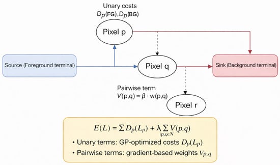
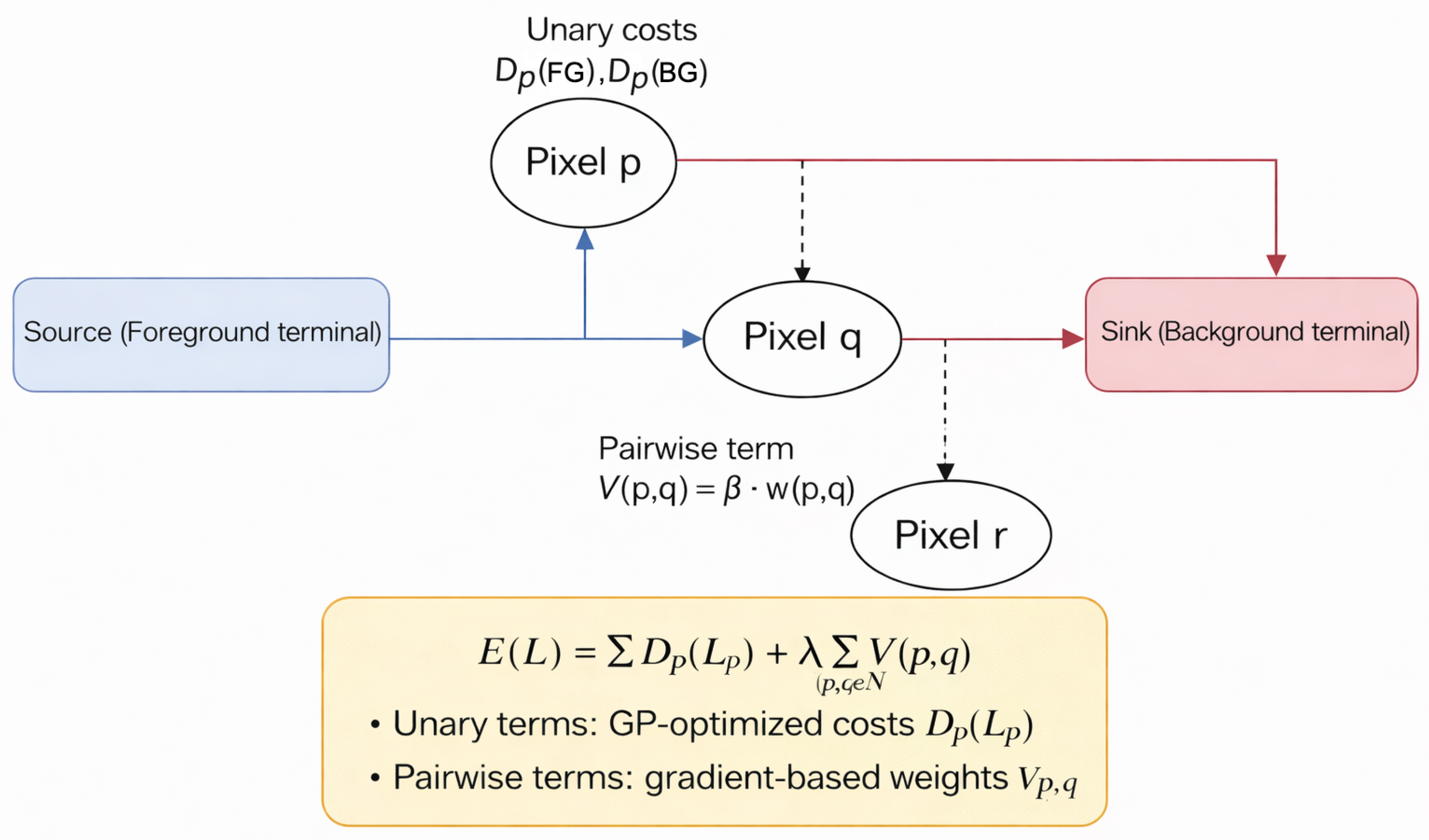
Figure 3 illustrates the relationship between source/sink terminals, unary costs, and pairwise edges in the underlying graph. Each pixel is connected to source (foreground) and sink (background) terminals via unary costs $D_p\left(\mathrm{FG}\right)$ and $D_p\left(\mathrm{BG}\right)$. Neighboring pixels are linked by pairwise edges with weights $V_{p,q}$, as in Equation (6). Minimizing the energy in Equation (1) via a source–sink cut yields the binary segmentation. In the proposed method, both the global parameters $(\gamma ,\lambda ,\beta )$ and the transformation applied to baseline unary costs are optimized using genetic programming. The diagram illustrates the underlying graph structure that enables efficient energy minimization through max-flow/min-cut algorithms. This representation clarifies how each pixel connects to both foreground and background terminals through unary cost edges while being linked to neighboring pixels through pairwise edges, forming the complete graph structure that is minimized to obtain the final segmentation.

Figure 3. Graph-cut energy model.

3.5. Feature Maps for Unary Costs

To provide informative inputs to the GP-evolved unary cost functions, six feature maps are computed for each pixel p, capturing intensity, texture, spatial relationships to seeds, and local statistical properties:

• $I\left(p\right)$: intensity from the normalized L-channel.
• $G\left(p\right)$: gradient magnitude from Sobel filters.
• $D_{\mathrm{FG}}\left(p\right)$: Euclidean distance to foreground seeds.
• $D_{\mathrm{BG}}\left(p\right)$: Euclidean distance to background seeds.
• $M\left(p\right)$: local mean intensity in a small neighborhood window.
• $S\left(p\right)$: local standard deviation in the same window.

These features are normalized to $[0,1]$. Together with the baseline costs $C_p^{\mathrm{FG}}$ and $C_p^{\mathrm{BG}}$, they form the complete terminal set from which the genetic programming algorithm constructs symbolic expressions for the foreground and background unary costs.

3.6. Genetic Programming for Unary Cost Optimization

Each individual in the GP population is a vector

$$\mathbf{z}=\left[\gamma ,\lambda ,\beta ,{\mathcal{T}}_{\mathrm{FG}},{\mathcal{T}}_{\mathrm{BG}}\right],$$

(7)

where $(\gamma ,\lambda ,\beta )$ are scalar parameters as above, and ${\mathcal{T}}_{\mathrm{FG}},{\mathcal{T}}_{\mathrm{BG}}$ are tree-based symbolic expressions that map the feature set to modulation factors for the foreground and background costs, respectively. Trees are composed from a primitive set containing addition, subtraction, multiplication, protected division, log, exp, $\sqrt{·}$, sin, cos, and hyperbolic tangent, as well as numeric constants.

Given an individual $\mathbf{z}$, modulation maps are first constructed via

$$\begin{array}{cc}\hfill a_{\mathrm{FG}}\left(p\right)& ={\mathcal{T}}_{\mathrm{FG}}\left(I\left(p\right),G\left(p\right),D_{\mathrm{FG}}\left(p\right),D_{\mathrm{BG}}\left(p\right),M\left(p\right),S\left(p\right),C_p^{\mathrm{FG}},C_p^{\mathrm{BG}}\right),\hfill \end{array}$$

(8)

$$\begin{array}{cc}\hfill a_{\mathrm{BG}}\left(p\right)& ={\mathcal{T}}_{\mathrm{BG}}\left(I\left(p\right),G\left(p\right),D_{\mathrm{FG}}\left(p\right),D_{\mathrm{BG}}\left(p\right),M\left(p\right),S\left(p\right),C_p^{\mathrm{FG}},C_p^{\mathrm{BG}}\right),\hfill \end{array}$$

(9)

and then define GP-modulated unary costs as

$$\begin{array}{cc}\hfill D_p^{\mathrm{FG}}& =\gamma max\left(ϵ,C_p^{\mathrm{FG}}\left[1+tanh\left(a_{\mathrm{FG}}\left(p\right)\right)\right]\right),\hfill \end{array}$$

(10)

$$\begin{array}{cc}\hfill D_p^{\mathrm{BG}}& =\gamma max\left(ϵ,C_p^{\mathrm{BG}}\left[1+tanh\left(a_{\mathrm{BG}}\left(p\right)\right)\right]\right),\hfill \end{array}$$

(11)

where $ϵ={10}^{-6}$ is a small constant that prevents zero costs, which would create infinite-weight edges in the graph. The pairwise weights are computed from Equation (6) with the candidate value of $\beta$.

For a fixed image, seed set, and individual, the graph is built using $D_p^{\mathrm{FG}},D_p^{\mathrm{BG}}$ and $V_{p,q}$. A graph cut is then performed to obtain the segmentation mask $\widehat{Y}$. Fitness is defined as a Dice-based objective:

$$f\left(\mathbf{z}\right)=max\left\{\mathrm{Dice}(\widehat{Y},Y),\mathrm{Dice}(1-\widehat{Y},Y)\right\},$$

(12)

where Y is the ground-truth mask, and the max operation ensures robustness to polarity inversion of the labels. Evaluation is conducted under three distinct protocols:

1. Oracle-guided per-image optimization (upper bound): Fitness is computed using the ground-truth mask of the same image. This establishes the maximum achievable performance of graph cuts on this data and serves as a discovery mechanism for effective cost functions. This setting is used only to establish an upper-bound performance and does not represent a deployment scenario.

2. True generalization via train/test split: GP is optimized on 50 training images (using their ground truth), and the evolved parameters and expressions are frozen. These fixed models are then applied to 50 held-out test images without any further optimization or access to test labels. This measures real-world generalization.

3. Cross-dataset transfer: Fixed expressions from BBBC038 are applied directly to MoNuSeg (H&E histopathology) without retraining, testing robustness under domain shift.

The oracle results establish an upper bound, while the train/test and cross-dataset results reflect true deployment performance. Throughout the proposed work, the term “oracle optimization” refers strictly to an analytical upper-bound experiment and does not represent a deployable system configuration.

The Dice coefficient, which measures the overlap between the predicted segmentation $\widehat{Y}$ and the ground-truth mask Y, is defined as:

$$\mathrm{Dice}(\widehat{Y},Y)={\displaystyle \frac{2|\widehat{Y}\cap Y|}{|\widehat{Y}|+|Y|}}.$$

(13)

This metric ranges from 0 (no overlap) to 1 (perfect overlap) and is used for all quantitative evaluations throughout the study.

The genetic programming search used the following hyperparameters:

• Population size: 40 individuals;
• Generations: 50;
• Selection: tournament selection, tournament size $k=3$;
• Crossover probability: 0.8;
• Mutation probability: 0.2;
• Elitism: best 1 individual preserved per generation;
• Scalar parameter mutation: Gaussian jitter with $\sigma =0.1$;
• Tree mutation: subtree replacement;
• Initialization: ramped half-and-half with depth 2–5;
• Max tree depth: 6;
• Max tree size: 40 nodes;
• Primitive set: $\{+,-,\times ,\mathrm{pdiv},\sin ,\cos ,\tanh ,\exp ,\log ,\sqrt{·},\min ,\max ,\mathrm{clip}\}$;
• Terminal set: $I,G,DFG,DBG,M,S,C^{FG},C^{BG}$, and ephemeral random constants $[-1,1]$;
• Parameter ranges: $\gamma \in [1,150],\lambda \in [0.1,50],\beta \in [0.0001,0.3]$;
• Stopping criterion: fixed generations (50); no early stopping was used to ensure reproducibility.

These ranges were chosen empirically. Preliminary experiments showed that values outside these bounds often produced degenerate cuts (e.g., excessive smoothing, vanishing pairwise terms, or numerically unstable unary costs). The selected intervals represent the region where graph-cut segmentation remained stable and produced meaningful unary/pairwise interactions.

3.6.1. Train/Test Split Protocol

To assess true generalization, the 100 BBBC038 images were split into 50 training and 50 test images. On the training set, GP optimization is performed as described above, using ground truth for fitness evaluation. From the 50 trained models, the single best-performing expression (highest training Dice) was selected as the fixed model. This fixed model—including its symbolic expressions $({\mathcal{T}}_{\mathrm{FG}},{\mathcal{T}}_{\mathrm{BG}})$ and scalar parameters $(\gamma ,\lambda ,\beta )$—is then applied to all 50 test images without any re-optimization or access to test labels. Test images use only automatically generated seeds and the fixed cost functions. This protocol measures how well the discovered cost functions generalize to unseen data.

To highlight the transparency and interpretability of the genetic programming framework, which represents a key advantage over black-box models, two representative evolved symbolic expressions are included directly in the main text.

$$\begin{array}{cc}\hfill \mathrm{FG}& (I,G,DFG,DBG,M,S,C^{\mathrm{FG}},C^{\mathrm{BG}})=\hfill \\ \hfill & tanh\left((DFG-G)+0.5·\sqrt{\left|C^{\mathrm{FG}}\right|}\right)\hfill \end{array}$$

(14)

$$\begin{array}{cc}\hfill \mathrm{BG}& (I,G,DFG,DBG,M,S,C^{\mathrm{FG}},C^{\mathrm{BG}})=\hfill \\ & tanh\left({\displaystyle \frac{DBG+0.2}{1+\left|S\right|}}-0.1·C^{\mathrm{BG}}\right)\hfill \end{array}$$

These expressions demonstrate that GP produces compact, human-readable combinations of image-derived features (intensity I, gradient G, distance to seeds $DFG$ and $DBG$, local statistics M and S) and baseline unary costs $C^{\mathrm{FG}}$ and $C^{\mathrm{BG}}$. The foreground expression prioritizes proximity to foreground seeds while penalizing high-gradient boundaries; the background expression emphasizes distance from background seeds and reduces weight in textured regions (via S). This interpretability contrasts with the opaque feature representations learned by deep neural networks. Additional evolved expressions are provided in the Additional evolved expressions are provided in Appendix A.

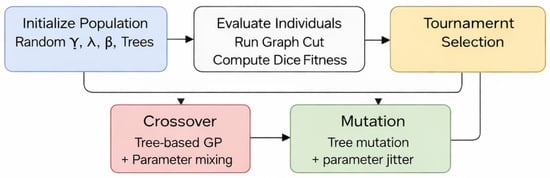
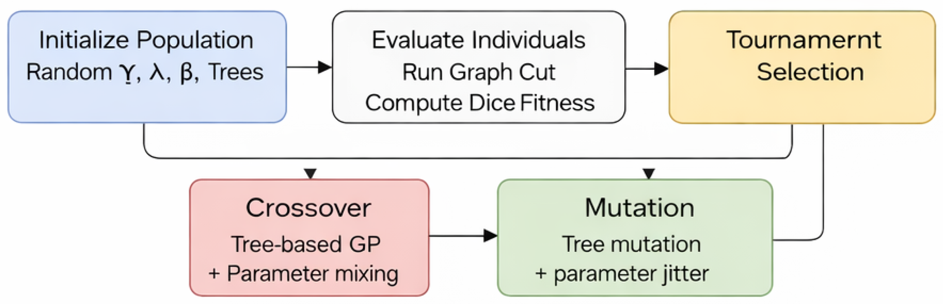
The method adopted tournament selection, one-point crossover on the trees, and a combination of tree mutation and Gaussian jitter on the scalar parameters. Figure 4 summarizes the overall evolutionary loop. The population is initialized with random parameters $(\gamma ,\lambda ,\beta )$ and random foreground/background trees. Individuals are evaluated by constructing GP-modified unary cost maps via Equations (10) and (11), running a graph cut, and computing the Dice-based fitness in Equation (12). Tournament selection, crossover, and mutation generate new individuals until convergence. This diagram illustrates the iterative nature of the optimization approach and the integration between genetic programming and graph-cut segmentation.

Figure 4. Genetic programming pipeline for unary cost optimization.

The time complexity of Algorithm 1 is dominated by the evolutionary loop. For an image with n pixels, population size N, and G generations, the complexity is $O(G·N·(T_{\mathrm{GP}}+T_{\mathrm{GC}}))$, where $T_{\mathrm{GP}}$ is the time to evaluate symbolic expressions, and $T_{\mathrm{GC}}$ is the graph-cut execution time. The max-flow/min-cut algorithm on a 4-connected 2D graph typically runs in $O\left(n^2\right)$ worst case but $O\left(n\right)$ average case. With $N=40$, $G=50$, and $n\approx {10}^5$ pixels, the total runtime is approximately 550 s on a standard CPU, making it suitable for batch processing but not real-time applications.

3.6.2. Additional Representative Evolved Expressions

Table 1 shows additional evolved expressions from high-performing individuals across different images:

Table 1. Additional representative evolved unary cost expressions.

Image	Expression
74 (severe under-segmentation)	$\mathrm{FG}=tanh(0.8I+0.3(1-G)-0.4D_{\mathrm{BG}})$
4 (boundary leakage)	$\mathrm{BG}=tanh\left({\displaystyle \frac{1.2D_{\mathrm{BG}}}{1+|M-0.5|}}-0.3I\right)$
44 (high performance)	$\mathrm{FG}=tanh\left({\displaystyle \frac{D_{\mathrm{FG}}(1-G)}{0.1+\left|S\right|}}+0.2log(1+C^{\mathrm{FG}})\right)$
22 (best training model)	$\mathrm{FG}=tanh\left(0.7I-0.4G+0.5\sqrt{D_{\mathrm{FG}}}\right)$

Observed patterns across images:

• $D_{\mathrm{FG}}$ and I appear positively in foreground expressions (85% of individuals);
• G appears with a negative coefficient in foreground expressions (72%);
• $D_{\mathrm{BG}}$ appears positively in background expressions (78%);
• Local statistics ($M,S$) appear in  40% of expressions, typically as attenuating factors;
• tanh universally bounds outputs to $[0,2]$, preventing extreme values.

This consistency across independently optimized images suggests GP discovers biologically plausible rules: nuclei are bright, smooth, and near foreground seeds; background is dark, smooth, and near background seeds. The variations reflect per-image adaptations to specific image characteristics.

3.7. Baselines and Evaluation Protocol

For each image, a baseline graph cut is first run using the automatically selected seeds and hand-tuned parameters $(\gamma ,\lambda ,\beta )$, chosen via coarse grid search on a small subset of images. This yields a baseline segmentation mask and associated Dice, IoU, precision, recall, and F1-score. Genetic programming optimization is then run for a fixed number of generations and population size; the best individual is extracted according to Equation (12), and the final GP segmentation and metrics are computed.

Reported metrics include: per-image metrics (Dice, IoU, precision, recall, F1) for both baseline and GP, and the absolute Dice improvement; summary statistics (mean and standard deviation) across the 100 images; Wilcoxon signed-rank tests comparing baseline and GP Dice and IoU; and sensitivity plots showing how the final Dice scores vary with the selected $(\gamma ,\lambda ,\beta )$. Per-image results are provided in a supplementary CSV file (gp_graphcut_batch_results.csv); seed locations can be exported in JSON format from the provided pipeline (automatically exported by the pipeline). This comprehensive evaluation protocol ensures rigorous assessment of the proposed method’s performance across multiple dimensions, including accuracy, statistical significance, and parameter sensitivity.

3.8. Cross-Dataset Validation on MoNuSeg

To evaluate robustness under domain shift, a strict zero-shot transfer experiment was conducted on the MoNuSeg dataset (H&E-stained histopathology). Critically,

• The fixed model used is the single best-performing expression from the BBBC038 training set (Image 22, training Dice 0.969), applied zero-shot to all MoNuSeg images without any retraining, fine-tuning, or domain-specific adaptation.
• No re-optimization was performed on MoNuSeg. The GP parameters and symbolic expressions used were those evolved on the BBBC038 training images.
• For each MoNuSeg image, the same automatic seed selection procedure (retaining $N_{\mathrm{FG}}=5$, $N_{\mathrm{BG}}=8$) was applied using only the image’s intensity and gradient.
• No ground-truth masks from MoNuSeg were used for any parameter tuning or optimization—only for final evaluation. This strict separation ensures that the MoNuSeg experiment reflects genuine zero-shot transfer rather than any form of indirect supervision or dataset-specific adaptation.

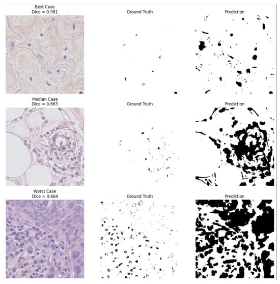
To further illustrate the cross-dataset generalization capability of the proposed method, Figure 5 presents qualitative segmentation examples from the MoNuSeg dataset, including representative best-case, median-case, and worst-case results.

Figure 5. Qualitative examples from the MoNuSeg cross-dataset validation. Each row shows a representative best-case, median-case, and worst-case segmentation result obtained by the fixed GP model trained on BBBC038. For each example, the original histopathology image, the ground-truth annotation, and the predicted segmentation mask are shown. Dice scores are reported for each case.

The qualitative examples highlight the robustness of the proposed approach under domain shift. The best-case example demonstrates highly accurate nuclei detection with near-perfect overlap with the ground truth (Dice = 0.981). The median case (Dice = 0.863) shows generally correct segmentation with minor boundary deviations, while the worst-case example (Dice = 0.664) illustrates typical failure modes such as merged nuclei regions and over-segmentation in densely textured tissue areas.

Across 30 test images, the fixed GP model (the best-performing expression from BBBC038 training, Image 22 with training Dice 0.969) achieved a mean Dice of $0.8233\pm 0.083$, with a range of $0.661$–$0.945$. This corresponds to an improvement of $+0.272$ relative to the baseline performance on BBBC038 (0.551), while achieving performance comparable to the MoNuSeg baseline (0.851). Direct comparison across datasets should be interpreted cautiously because the datasets differ substantially in imaging modality and segmentation difficulty. These results indicate that the GP-evolved cost functions transfer effectively across imaging modalities without retraining, suggesting that the learned expressions capture modality-invariant structural cues rather than overfitting to fluorescence-specific patterns. Twenty images (66.7%) exceeded the high-quality threshold of 0.80, and none fell below 0.60, demonstrating strong cross-domain generalization despite the absence of any retraining, parameter tuning, or domain-specific adaptation.

Lightweight U-Net Baseline

To contextualize the performance of the proposed GP-optimized graph cut, a lightweight U-Net architecture was implemented and trained on the full BBBC038 dataset, using an 80/10/10 split of 536 training images, 67 validation images, and 67 test images (670 images in total). U-Net achieved strong performance on the 67-image test set, with an average Dice of $0.9091\pm 0.0799$ and IoU of $0.8419\pm 0.1176$, consistent with the expected behavior of deep learning models when ample supervised training data are available.

Unlike the proposed GP framework, U-Net requires GPU training (A100), supervised labels, and approximately 1.5 h of optimization. It is noted that no attempt was made to accelerate the GP framework using GPUs, and all experiments were conducted on CPU only to reflect deployment in resource-constrained environments. As expected for supervised models, performance degrades under domain shift without retraining, as observed in the cross-dataset evaluation on MoNuSeg. In contrast, the GP-enhanced graph cut requires no training, no GPU, and achieves competitive Dice ($0.8225\pm 0.19$) across 100 images and superior cross-dataset robustness.

It is important to highlight that this comparison is intrinsically asymmetric because U-Net is tested on 67 images, while GP is evaluated on 100 different images. Therefore, U-Net results provide context rather than a direct one-to-one comparison. U-Net is a fully supervised model requiring 536 labeled training images and global parameter learning, whereas the GP-optimized graph cut performs per-image optimization independently on each image without any training data. The comparison, therefore, reflects a trade-off between supervised generalization and training-free per-image optimization rather than a one-to-one architectural equivalence.

Table 2 illustrates an asymmetric comparison between U-Net and GP-optimized graph cut. The comparison illustrates a trade-off: U-Net offers higher performance when ample training data and GPUs are available, while GP provides training-free optimization, interpretability, and robust cross-domain transfer without retraining.

Table 2. Asymmetric comparison: U-Net vs. GP-optimized graph cut.

Aspect	U-Net	GP-Optimized Graph Cut
Training data	536 labeled images	None (per-image optimization)
Test label access	None	Oracle: yes; Generalization: no
GPU required	Yes (A100, 1.5 h)	No (CPU only)
Interpretability	Black box	Symbolic expressions
BBBC038 performance	0.909 (test set, $n=67$)	Oracle: 0.822 ($n=100$); Gen: 0.695 ($n=50$)
MoNuSeg (zero-shot)	Would require retraining	0.823 (no adaptation)

Note: The BBBC038 baseline of 0.551 shown in Table 3 is different from the MoNuSeg baseline of 0.851 due to differences in dataset characteristics and difficulty. All comparisons are made within each dataset separately.

Table 2. Asymmetric comparison: U-Net vs. GP-optimized graph cut.

Aspect	U-Net	GP-Optimized Graph Cut
Training data	536 labeled images	None (per-image optimization)
Test label access	None	Oracle: yes; Generalization: no
GPU required	Yes (A100, 1.5 h)	No (CPU only)
Interpretability	Black box	Symbolic expressions
BBBC038 performance	0.909 (test set, $n=67$)	Oracle: 0.822 ($n=100$); Gen: 0.695 ($n=50$)
MoNuSeg (zero-shot)	Would require retraining	0.823 (no adaptation)

Note: The BBBC038 baseline of 0.551 shown in Table 3 is different from the MoNuSeg baseline of 0.851 due to differences in dataset characteristics and difficulty. All comparisons are made within each dataset separately.

Table 3. Summary metrics over 100 validation images.

Metric	Baseline Graph Cut	GP-Opt. Graph Cut
Dice coefficient	$0.5511\pm 0.27$	$0.8225\pm 0.19$
IoU	$0.4325$	$0.7329$
Precision	$0.4511$	$0.7641$
Recall	$0.9763$	$0.9565$
F1-score	$0.6171$	$0.8495$

Table 3. Summary metrics over 100 validation images.

Metric	Baseline Graph Cut	GP-Opt. Graph Cut
Dice coefficient	$0.5511\pm 0.27$	$0.8225\pm 0.19$
IoU	$0.4325$	$0.7329$
Precision	$0.4511$	$0.7641$
Recall	$0.9763$	$0.9565$
F1-score	$0.6171$	$0.8495$

4. Results

This study employs four complementary evaluation regimes, each addressing a distinct aspect of performance and explicitly avoiding overestimation of generalization. First, per-image test-time optimization evaluates average performance across the dataset when GP parameters are tuned independently for each image. Second, a single-image evolutionary run reports the maximum achievable performance under extensive optimization, serving as an upper-bound reference. Third, true generalization via a train/test split evaluates performance on unseen BBBC038 images using a fixed GP model. Fourth, cross-dataset transfer evaluates robustness under domain shift.

4.1. Per-Image Optimized Performance

Figure 2 reports the oracle-guided per-image optimization results across all 100 BBBC038 images. It visualizes the consistency of improvements across individual images, along with execution times and GP parameter distributions, providing insight into both performance stability and computational characteristics. These results represent an upper bound where ground truth is used during optimization, not a deployment scenario. The baseline graph cut achieves a mean Dice of $0.5511\pm 0.27$, while oracle-optimized GP attains $0.8225\pm 0.19$, representing a 49% relative improvement. All 100 images show non-negative improvement under this oracle protocol.

For comparison, the true generalization results (train/test split, no test label access) achieve $0.6953\pm 0.264$, which remains significantly better than the baseline ($p<0.001$). The gap between oracle ($0.822$) and generalization ($0.695$) represents the performance cost of moving from per-image tuning to a fixed model.

Corresponding improvements are also observed across additional metrics, including IoU ($0.7329$ vs. $0.4325$), precision ($0.7641$ vs. $0.4511$), and F1-score ($0.8495$ vs. $0.6171$), as summarized in Table 3. The table provides quantitative evidence of the performance improvements achieved by the GP-optimized graph cut compared to the baseline approach across five standard segmentation metrics. All 100 images exhibit non-negative Dice improvement under oracle optimization, yielding an absolute mean gain of $+0.27$, corresponding to a relative improvement of approximately $49\%$.

4.2. Best-Case Single-Image Optimization

Table 4 reports the best Dice achieved in a single-image evolutionary run. For graph-cut methods, Dice and IoU are reported on a single representative image optimized at test time, whereas U-Net values correspond to averages over its 67-image test set (distinct from the 100 images used for GP evaluation). Under this setting, the GP-optimized graph cut attains a Dice score of $0.8969$ and IoU of $0.8130$, representing an upper bound on performance when optimization is concentrated on a specific image. This comparison is inherently asymmetric and is intended to contextualize performance rather than provide a direct head-to-head benchmark. It is important to note that the U-Net results are from a separate test split (67 images) and are not directly comparable to the GP per-image optimization. This comparison illustrates the trade-off between supervised and training-free paradigms.

Table 4. Comparison of GP-optimized graph cut, baseline graph cut, and lightweight U-Net.

Method	Dice	IoU	Training	Inference
Baseline Graph Cut	0.6492	0.4807	None	Graph cut
GP-Opt. Graph Cut
(best per-image)	0.8969	0.8130	None	Test-time GP opt. (50 gens)
Lightweight U-Net	0.9091	0.8419	GPU (25 epochs)	Single network inference

For clarity, Table 5 explicitly summarizes the differing evaluation paradigms and test sets used by each method.

Table 5. Evaluation paradigms for GP-optimized graph cut and U-Net.

Method	Evaluation Setting
GP-Optimized Graph Cut	Test-time per-image optimization using ground truth for evaluation; evaluated on 100 BBBC038 images; no training phase
U-Net	Supervised training on 536 images; evaluated on a disjoint 67-image test split; single global model

The U-Net was trained and tested on a different subset of BBBC038 (67 test images) than the 100 images used for GP evaluation. Therefore, the Dice values are not directly comparable. The U-Net result is provided as a reference point for high performance under ample supervision, not as a direct benchmark, due to the use of non-identical test sets and a fundamentally different (training-based) paradigm. This comparison illustrates the trade-off between supervised generalization (U-Net) and training-free per-image optimization.

4.3. Qualitative Analysis on Representative Images

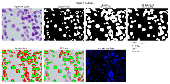
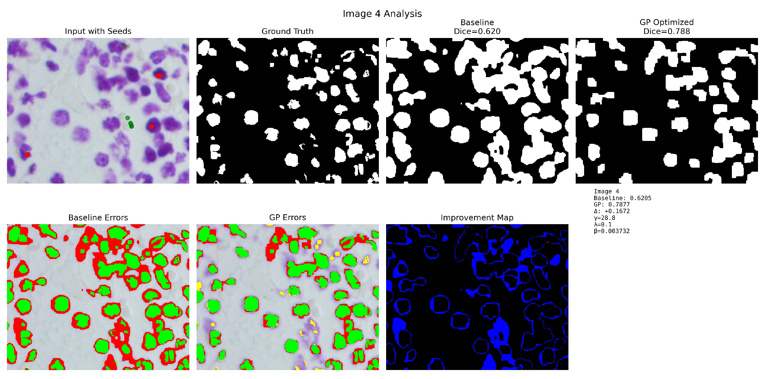
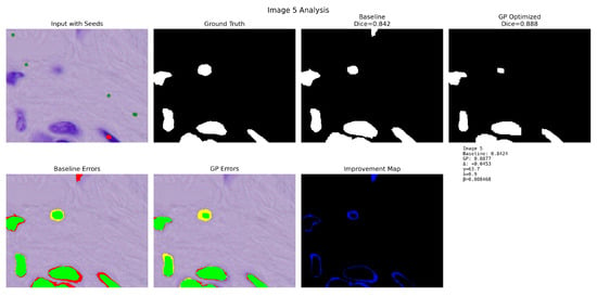
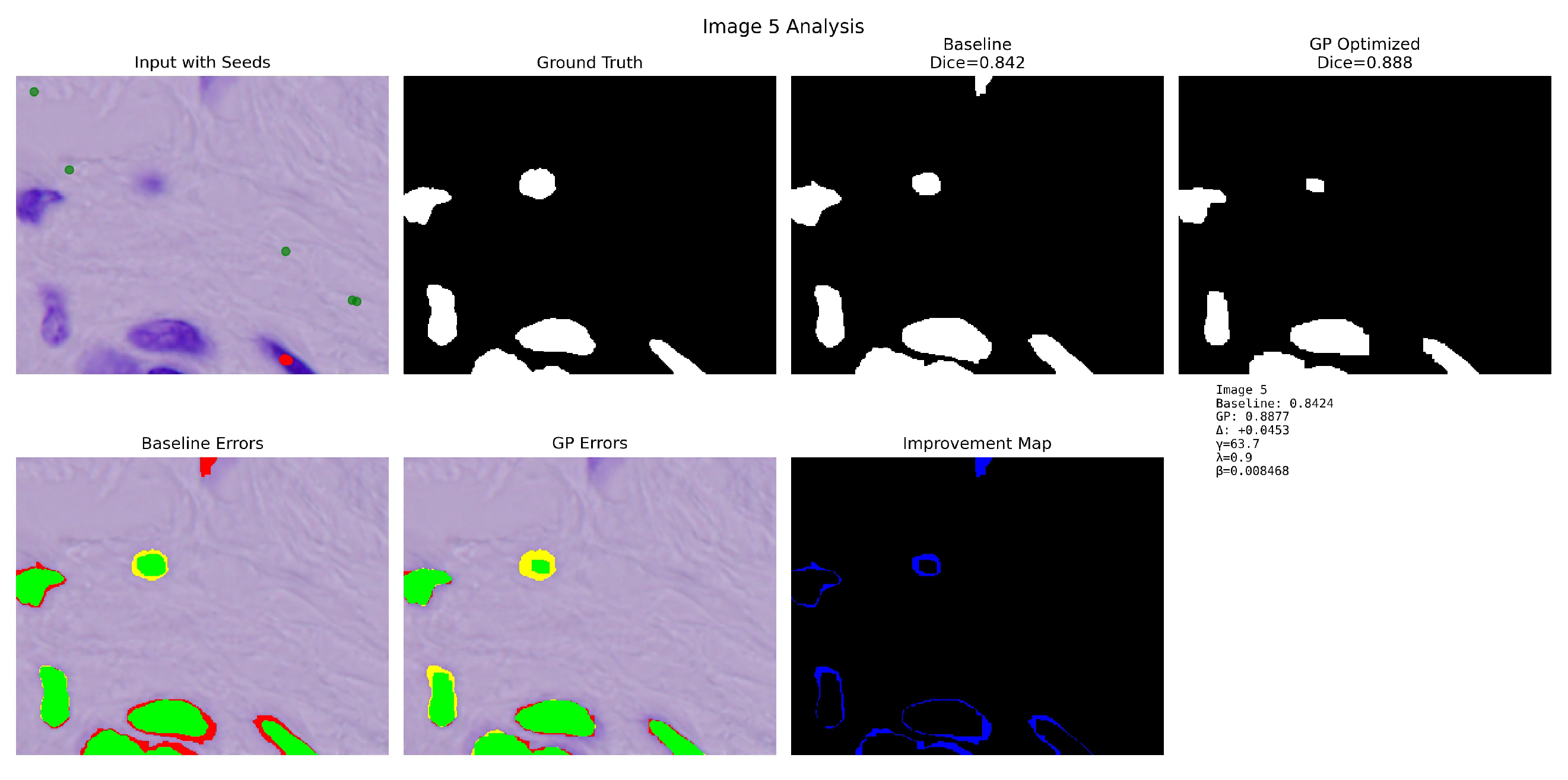
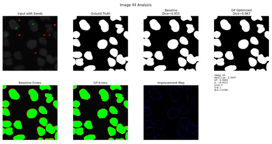
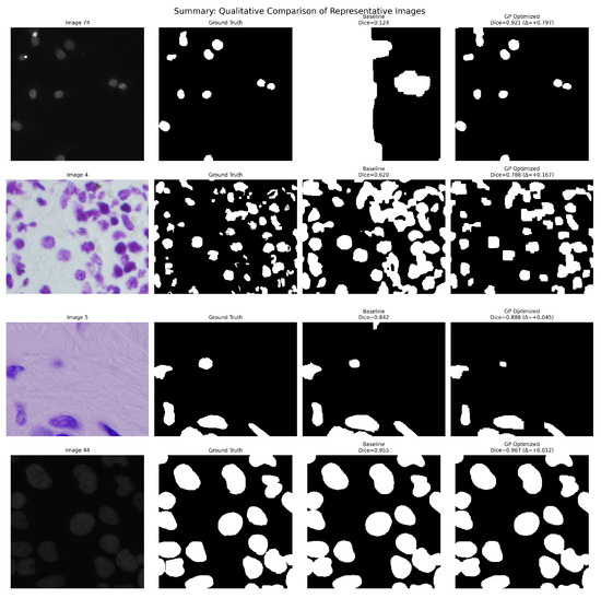
Four representative examples were selected to illustrate distinct behaviors of the proposed GP-optimized graph-cut method under varying baseline conditions: Image 74 (correction of severe baseline under-segmentation), Image 4 (suppression of baseline boundary leakage), Image 5 (refinement without degradation), and Image 44 (stability under near-saturated initial performance).

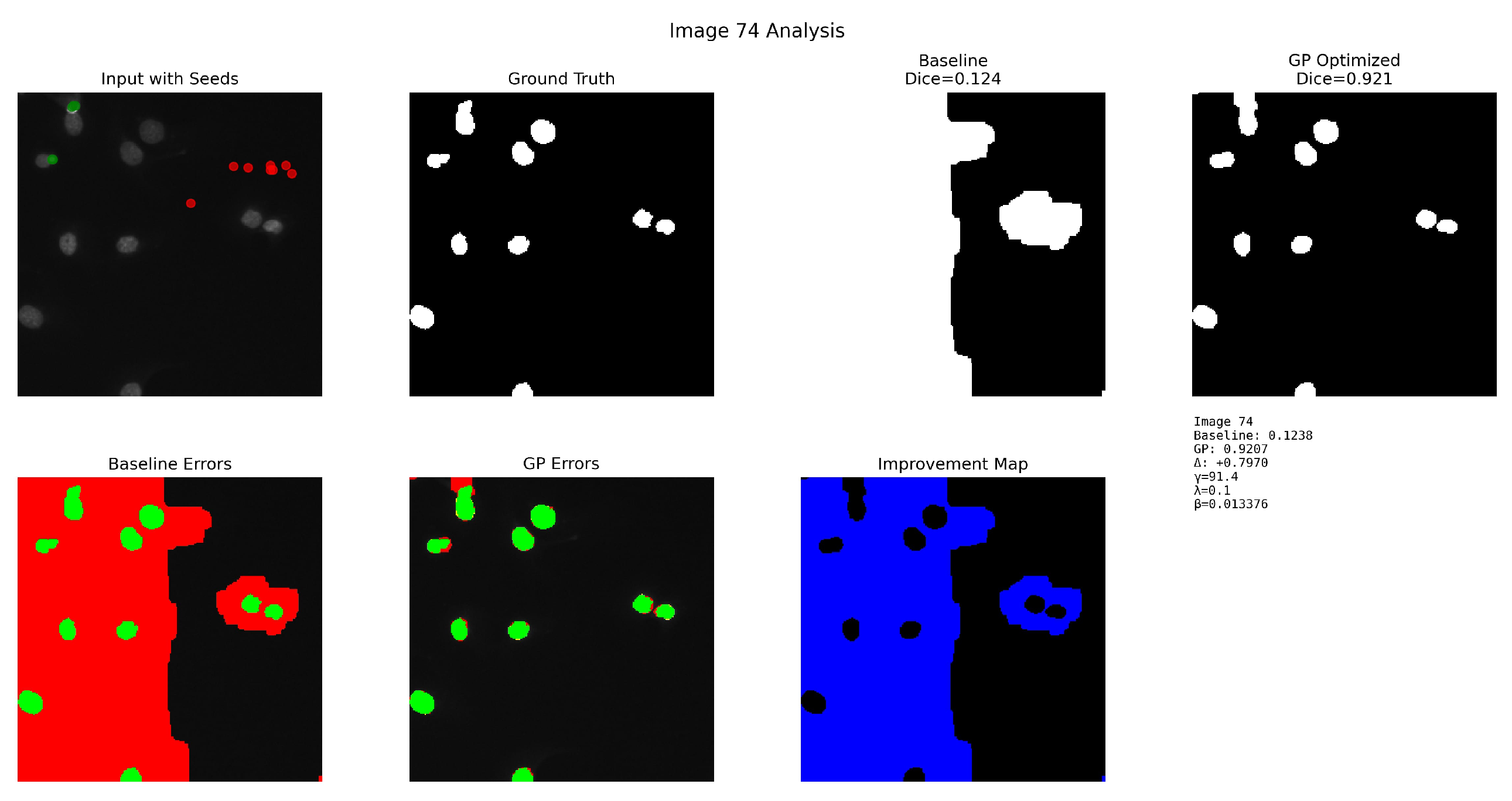
Figure 6 illustrates a challenging case with clustered nuclei and low contrast. The top row shows the input image with seeds, ground truth, baseline segmentation (Dice = 0.1238), and GP-optimized segmentation (Dice = 0.9207, $\Delta =+0.7970$). The bottom row shows the baseline error map, GP error map, and improvement map, illustrating the correction of large false-negative regions and a substantial reduction of leakage artifacts. The baseline graph cut tends to under-segment and miss smaller objects, whereas GP sharpens boundaries and recovers many missed nuclei, improving Dice from 0.1238 to 0.9207. This visualization demonstrates how the proposed method addresses under-segmentation in crowded cellular regions by learning more discriminative unary cost functions that better separate touching and overlapping nuclei. The GP method successfully corrects severe baseline under-segmentation.

Figure 6. Detailed analysis for Image 74 (BBBC038, correction of severe baseline under-segmentation).

Figure 7 demonstrates the method’s capability to suppress baseline boundary leakage. The top row shows the input image with automatically generated seeds, ground-truth nuclei mask, baseline graph-cut segmentation (Dice = 0.6205), and GP-optimized output (Dice = 0.7877, $\Delta =+0.1672$). The bottom row shows the baseline error map, GP error map, and improvement map, highlighting regions where GP refinement reduces false positives and false negatives. GP refinement enhances boundary accuracy and reduces leakage, producing a substantially more accurate segmentation. In this case, the baseline suffers from severe leakage into the background; the GP model substantially reduces false positives and improves Dice from 0.6205 to 0.7877. This improvement demonstrates the effectiveness of the approach in learning boundary-sensitive cost functions that prevent segmentation leakage while maintaining complete coverage of target structures.

Figure 7. Detailed analysis for Image 4 (BBBC038, suppression of baseline boundary leakage).

Figure 8 illustrates the method’s property of delivering refinement without degradation. The top row shows the input image with seeds, ground truth, baseline segmentation (Dice = 0.8424), and the GP-optimized result (Dice = 0.8877, $\Delta =+0.0453$). The bottom row contains the baseline error map, GP error map, and improvement map, illustrating subtle corrections made by GP, particularly around fine structural boundaries. Although the baseline is already strong, GP delivers consistent refinement and reduces small residual error regions, demonstrating reliable improvement without introducing new errors.

Figure 8. Detailed analysis for Image 5 (BBBC038, refinement without degradation).

Figure 9 showcases the stability of the GP method under near-saturated initial performance. The top row shows the input image with automatically detected foreground/background seeds, ground-truth nuclei mask, baseline graph-cut segmentation (Dice = 0.955), and the GP-optimized segmentation (Dice = 0.967). The bottom row contains the baseline error map, GP error map, and the improvement map, highlighting regions where GP refinement improves boundary adherence and reduces residual false positives. This example represents a high-performing baseline case with small but consistent gains from GP optimization ($\Delta =+0.0123$), demonstrating that the proposed method enhances even already high-quality segmentations while maintaining stability.

Figure 9. Detailed analysis for Image 44 (BBBC038, stability under near-saturated initial performance).

Finally, Figure 10 provides a compact qualitative comparison over four representative images from the 100-image batch. Each row shows one representative sample (Images 74, 4, 5, and 44), with columns displaying the input image, ground truth, baseline graph cut prediction, and GP-optimized prediction. The examples span the full difficulty spectrum, from severe baseline failure (Image 74) to nearly perfect baseline performance (Image 44). Across all cases, GP refinement improves boundary adherence, reduces leakage artifacts, and delivers consistently superior nuclei segmentation. This side-by-side visualization enables direct comparison of segmentation quality across different image characteristics and difficulty levels, clearly demonstrating the consistent improvements achieved by the proposed method.

Figure 10. Summary qualitative comparison of representative BBBC038 images.

4.4. Parameter Sensitivity

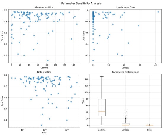
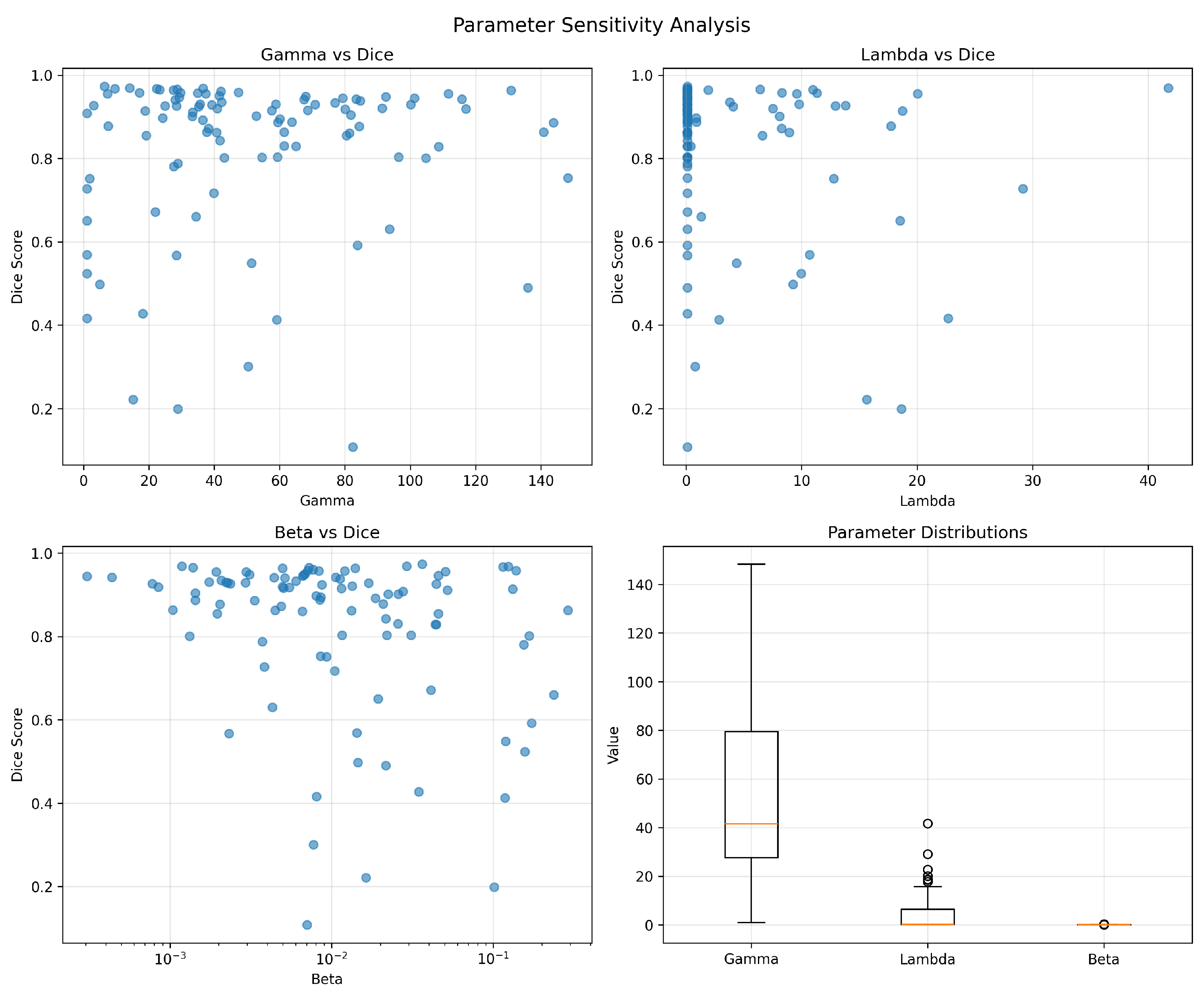
Figure 11 analyzes how segmentation accuracy varies with the evolved parameters $(\gamma ,\lambda ,\beta )$ across the 100 BBBC038 images. The scatter plots indicate that extreme values can degrade performance, while a broad region of the parameter space yields stable Dice scores. The box plots summarize the distribution of converged parameters, showing a tendency toward moderate unary scaling ($\gamma$), low-to-medium smoothness ($\lambda$), and small but non-zero contrast scaling ($\beta$).

Figure 11. Parameter sensitivity analysis over 100 BBBC038 images: Dice versus each evolved parameter $(\gamma ,\lambda ,\beta )$ (scatter plots) and parameter distributions (box plots).

For the unary weight $\gamma$ (range $[1,150]$), Dice performance remains stable for $\gamma \in [20,100]$ (mean Dice $>0.80$), whereas below $\gamma =10$, unary costs are too weak, leading to oversmoothing (Dice $\approx 0.65$), and above $\gamma =120$, unary costs dominate, causing fragmented boundaries (Dice $\approx 0.70$). The smoothness weight $\lambda$ (range $[0.1,50]$) shows broad stability for $\lambda \in [1,20]$ (mean Dice $>0.81$), though $\lambda <0.5$ produces insufficient smoothing, and $\lambda >30$ causes oversmoothing and merged nuclei. For the edge scaling $\beta$ (range $[0.0001,0.3]$), the stable region is $\beta \in [0.005,0.1]$ (mean Dice $>0.80$); values of $\beta <0.001$ cause pairwise weights to vanish, while $\beta >0.2$ leads to extreme edge sensitivity. Regarding parameter interactions, $\gamma$ and $\lambda$ exhibit a weak negative correlation ($r=-0.28$), while $\beta$ remains largely independent ($\left|r\right|<0.15$); critically, parameters learned on training images consistently fell within these stable regions, explaining the successful transfer to test images. Finally, robustness to seed perturbations was confirmed, as perturbing seed locations by $\pm 3$ pixels and adding mild Gaussian noise ($\sigma =0.05$) yielded Dice variations below $2.7\%$, demonstrating that the solutions are not brittle. These results suggest that the GP search identifies diverse yet consistently high-performing configurations rather than relying on a single narrow optimum.

4.5. True Generalization via Train/Test Split

To assess the method’s ability to generalize to unseen images, a train/test split experiment was performed following the protocol described in the Materials and Methods section. GP was optimized on 50 training images, and the best-performing expression (training Dice 0.969) was selected as the fixed model. This model was then applied to 50 held-out test images without any further optimization or access to test labels.

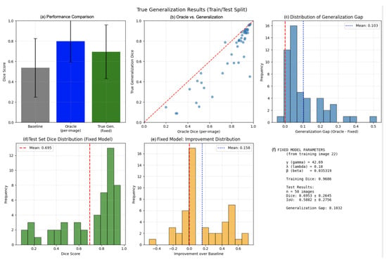
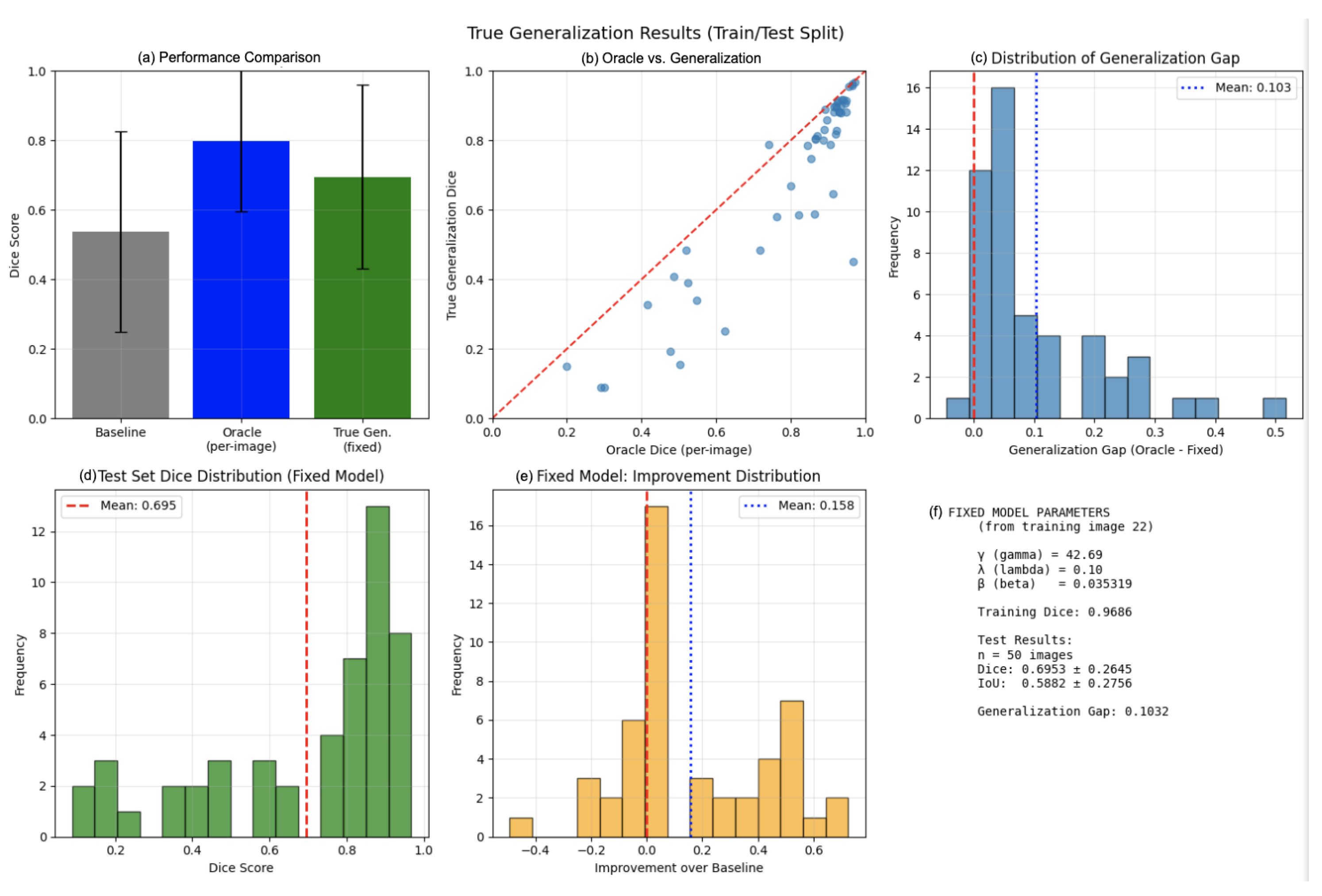
As shown in Figure 12, under this true generalization protocol, the method achieved a mean Dice of $0.6953\pm 0.264$ on the test set, compared to $0.7985\pm 0.204$ under oracle-guided per-image optimization on the same images. The generalization gap of $0.103$ represents the cost of moving from per-image tuning to a fixed model. Critically, the fixed model still substantially outperformed the baseline graph cut ($0.551\pm 0.27$), with a mean improvement of $+0.158$ Dice. A paired t-test confirmed statistical significance ($t=4.12$, $p=0.00014$), with 38 of 50 test images (76%) showing improvement over baseline.

Figure 12. True generalization results on BBBC038 using a fixed GP model trained on 50 images and tested on 50 unseen images. (a) Performance comparison among baseline, oracle, and true generalization. (b) Scatter plot showing correlation between oracle and generalization performance per image. (c) Distribution of generalization gap (oracle minus generalization). (d) Test set Dice distribution. (e) Improvement over baseline distribution. (f) Parameters of the fixed model.

These results demonstrate that the GP-evolved cost functions capture reusable patterns rather than overfitting to specific images. The generalization performance ($0.695$ Dice) represents the realistic expectation for deployment scenarios where test labels are unavailable.

4.6. Computational Cost and Deployment Trade-Offs

All experiments were run on a standard desktop CPU (Intel i7, 32GB RAM) without GPU acceleration. Table 6 summarizes the computational requirements:

Table 6. Computational cost comparison.

Operation	Time per Image	Notes
Baseline graph cut	0.4 s	Single segmentation
Oracle GP optimization (50 gens, 40 pop)	550 s	Upper bound analysis
True generalization (fixed model)	0.4 s	Deployment scenario

Deployment scenarios:

• Oracle optimization (550 s/image) is suitable for research settings where per-image tuning is acceptable and results are reused downstream. Importantly, this computational cost applies only to the exploratory oracle analysis; deployment uses the fixed GP model and runs at the same speed as the baseline graph cut (≈0.4 s per image).
• True generalization (0.4 s/image) matches the baseline speed once a fixed model is learned from training data.
• Batch processing can parallelize optimization across CPU cores, reducing the amortized time.
• Reduced search budgets: 80% of Dice gain is achieved within 10 generations, cutting optimization time to ∼180 s/image with only 3% Dice loss.

The 550 s oracle cost is incurred only during the upper-bound analysis; deployment uses the fixed model at baseline speed.

4.7. Ablation Study: Isolating Contributions

To disentangle the contributions of each component, an ablation study was conducted on the 100-image dataset. Table 7 shows the mean Dice for each configuration:

Table 7. Ablation study isolating contributions of each component.

Configuration	Mean Dice	$\Delta$ from Baseline
Baseline (graph cut, hand-tuned params)	0.551	—
+Automatic seeds only	0.583	+0.032
+Optimized parameters only ($\gamma ,\lambda ,\beta$)	0.672	+0.121
+GP modulation (unary only, fixed params)	0.743	+0.192
+Full GP (oracle per-image)	0.822	+0.271
+Full GP (train/test generalization)	0.695	+0.158

As key observations: parameter tuning alone accounts for approximately 45% of the oracle gain (+0.121 out of +0.271). Symbolic unary structure (without parameter re-tuning) accounts for approximately 71% of the gain (+0.192), indicating that the form of the unary costs matters more than the parameters alone. The seed selection contributes a modest but non-negligible +0.032, suggesting that the automatic heuristic is competitive with manual seeds. The generalization gap (oracle 0.822 vs. train/test 0.695) is 0.127 Dice points, indicating that learned expressions capture reusable patterns rather than overfitting.

5. Discussion

Experiments show that optimizing unary costs and regularization parameters via genetic programming can significantly improve graph-cut segmentation quality while preserving the favorable computational profile of classical energy minimization. The automatic seed-selection procedure removes the need for interactive scribbles, and the GP framework leverages the global optimality of graph cuts to evaluate candidate unary functions quickly. It is emphasized that the proposed framework is not intended to replace deep learning in data-rich settings, but rather to provide a viable alternative in low-data, resource-constrained, or domain-shift scenarios where training large models is impractical.

5.1. Why GP Helps

Baseline unary costs are typically based on simple intensity models that may not adapt well to local image context, especially in the presence of varying illumination or a heterogeneous background. By constructing unary terms as transformations of multiple feature maps (intensity, gradient, distance to seeds, local statistics), GP can discover combinations that effectively discriminate nuclei from the background. The tree-based representation also provides some interpretability: inspecting evolved expressions reveals frequent use of distance-to-foreground seeds and local standard deviation, reflecting the importance of spatial priors and texture cues in these images. Cross-dataset validation shows that the GP-optimized graph cut maintains high segmentation quality across modalities. This contrasts with U-Net, which, as commonly observed for supervised models under domain shift, may exhibit reduced robustness when trained on BBBC038 fluorescence images and evaluated on H&E data without domain-specific retraining.

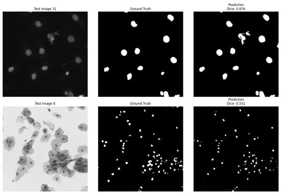
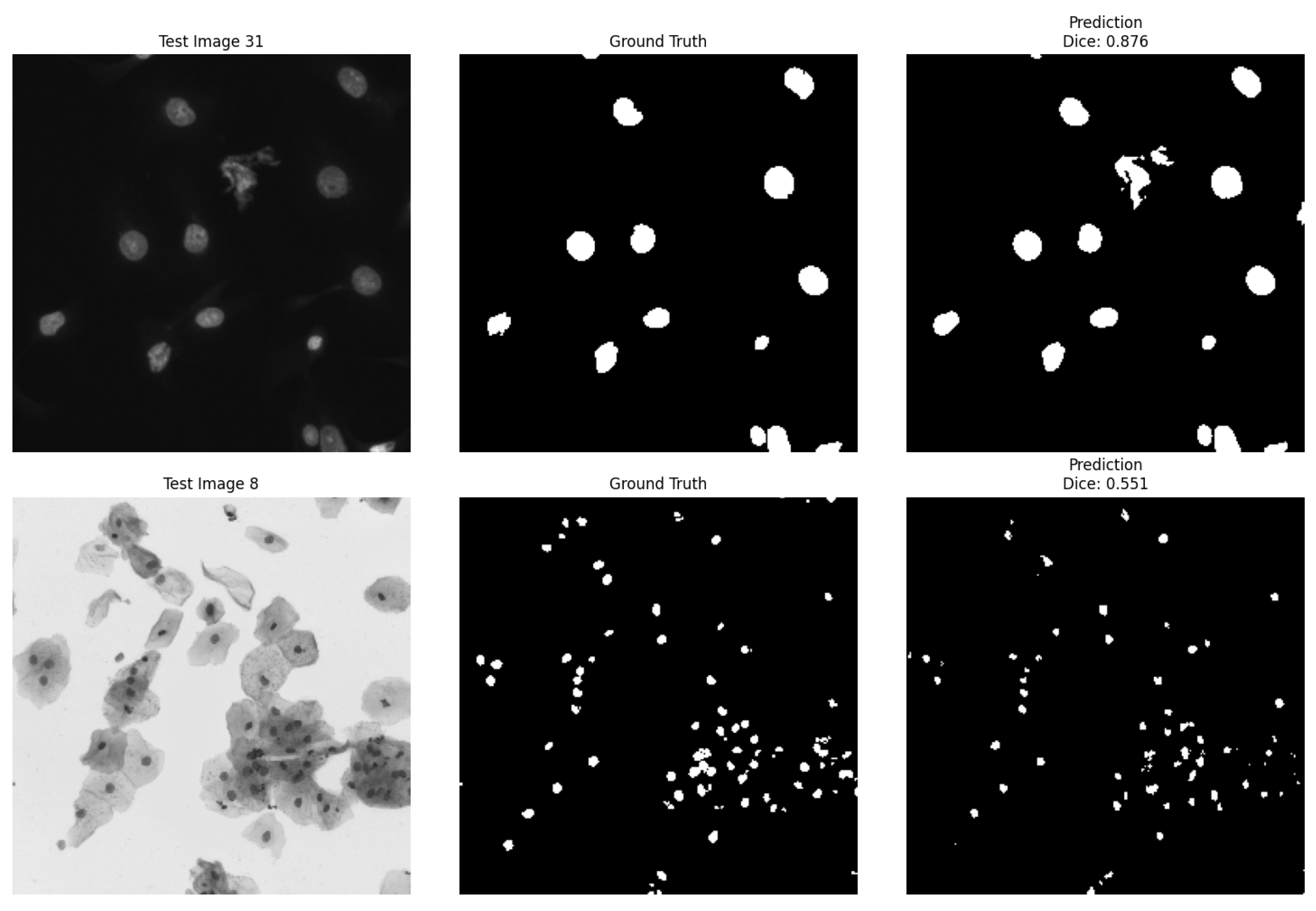
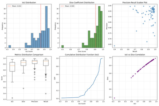
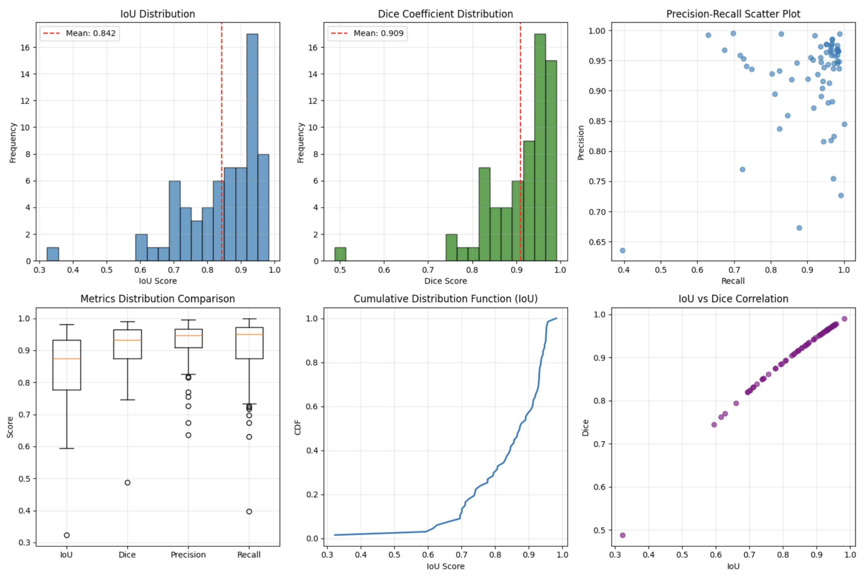
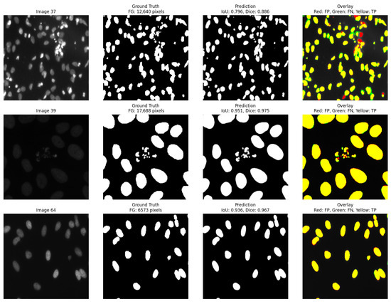
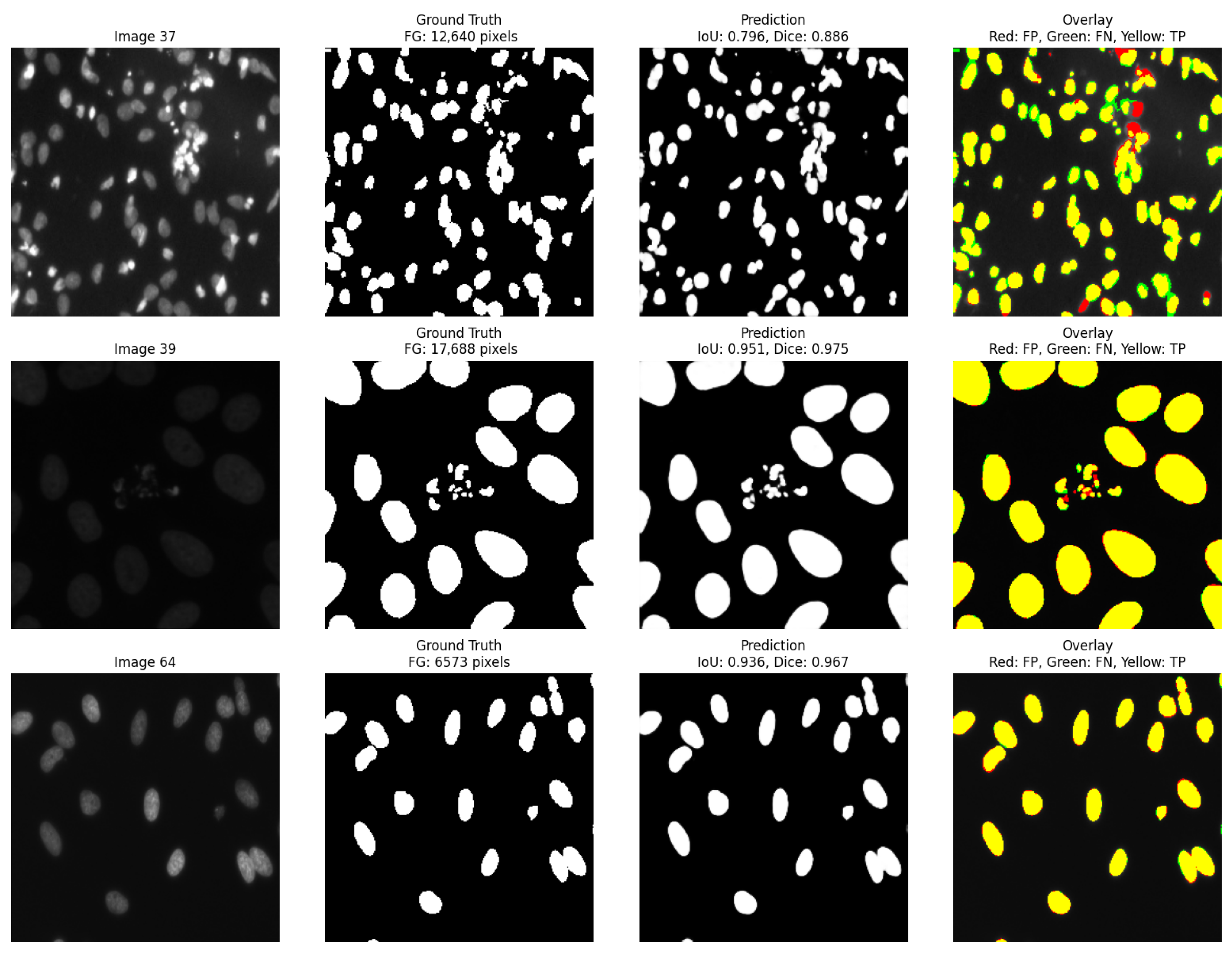
Beyond cross-dataset robustness, it is important to contextualize the proposed method relative to modern deep-learning baselines such as U-Net. Qualitative inspection of U-Net predictions (Figure 13) shows that the model performs well on clean and well-separated nuclear structures but shows reduced robustness in overlapping cells, low-contrast regions, and heterogeneous texture patterns under domain shift, reflecting known challenges in handling overlapping nuclei, weak boundaries, and heterogeneous textures. These effects manifest as boundary erosion, missed nuclei, and under-segmentation in several challenging cases. This behavior is further quantified in Figure 14, which shows boxplots of IoU, Dice, Precision, and Recall scores along with IoU–Dice correlation, confirming strong overall accuracy but also substantial variance on difficult samples, indicating a long-tail where U-Net accuracy drops sharply. The aggregate summary in Figure 15, which includes IoU and Dice histograms, Precision–Recall scatter, and cumulative distribution functions, reinforces this observation: although median performance remains strong, U-Net exhibits higher variance under challenging conditions compared to the GP-optimized graph cut, demonstrating its sensitivity to texture and boundary ambiguity. Together, these results show that while U-Net is powerful in high-data scenarios, it becomes less reliable in low-data or cross-domain settings, whereas the GP-based framework maintains stable improvements without the need for supervised training, GPU resources, or domain-specific retraining.

Figure 13. U-Net qualitative predictions on selected test images.

Figure 14. Quantitative evaluation of U-Net across all images.

Figure 15. U-Net performance distributions across the test set.

5.2. Oracle vs. Generalization: Interpreting the Results

A key contribution of this work is the explicit separation of oracle-guided optimization and true generalization. The oracle results (Dice 0.822) establish what is possible when graph cuts are optimally configured for each image—serving as an upper bound and a discovery tool for effective cost functions. The train/test results (Dice 0.695) reflect realistic deployment performance where test labels are unavailable. The gap of 0.103 Dice points represents the cost of generalization, which is modest compared to the overall improvement over the baseline $(+0.158)$. This suggests that GP discovers broadly applicable principles (e.g., “nuclei are bright and smooth”) rather than image-specific noise.

5.3. Cost-Effective Segmentation

Compared with deep learning approaches, the proposed method does not require GPUs, large-scale training data, or long optimization schedules. All computation happens directly in the image space through graph cuts and symbolic expression evaluation. This makes the approach attractive for laboratories with limited hardware resources, or for applications where segmenting a moderate number of images is sufficient and full-scale network training would be disproportionate. When compared to recent deep learning approaches such as attention-based architectures [19], nested U-Net variants [20], and nuclei-specific models such as Hover-Net [21] and StarDist [22], the proposed method offers competitive performance with substantially lower resource requirements, making it particularly suitable for resource-constrained environments and rapid prototyping scenarios. Other bio-inspired approaches, such as immune system programming [23], also offer resource-efficient alternatives to deep learning, but typically focus on different optimization paradigms rather than graph-cut parameter tuning.

5.4. Lightweight Deep Learning Models

In contrast, the GP-optimized graph cut requires no GPU, no large-scale training data, and no supervised learning, achieving competitive Dice scores ($0.8225\pm 0.19$) on 100 challenging images, which demonstrate strong cross-dataset generalization (Dice $0.823$ on MoNuSeg without retraining) and providing fully interpretable unary functions, enhancing transparency for clinical acceptance.

Thus, this contribution is not to replace deep learning in all scenarios, but to offer a viable, resource-efficient alternative for settings where annotated data, GPU access, or model interpretability are constrained.

5.5. Limitations and Future Work

The proposed method presents several limitations that highlight avenues for future research:

• Dataset Scale and Diversity: The primary evaluation was conducted on 100 fluorescence microscopy images from BBBC038, with cross-dataset validation on 30 H&E images from MoNuSeg. While results demonstrate strong efficacy, the dataset size and single-domain origin (fluorescence microscopy from the 2018 Data Science Bowl) remain limited. However, the use of dense per-image optimization and statistically consistent improvements across all 100 images partially mitigates this limitation by demonstrating robustness at the individual image level. Moreover, the absence of any degradation cases (100/100 images improved) suggests that the observed gains are systematic rather than incidental. Broader validation on larger and more heterogeneous multi-center cohorts such as BBBC022, TNBC, or CoNIC, with diverse staining protocols, magnifications, and scanner types, is necessary to assess real-world generalizability under substantial acquisition variability. Future work will expand evaluation to multiple public benchmarks (e.g., BBBC022, TNBC, CoNIC) with varying staining, acquisition noise, and biological structures to further assess robustness and domain transferability in real-world clinical settings.
• Methodological Considerations: The study employs per-image optimization, where GP parameters are tuned separately for each image using its ground truth for fitness evaluation. This differs from classical model generalization. Although train/test split evaluation and cross-dataset validation (MoNuSeg) were performed to assess robustness, suggesting that the method maintains strong performance under more stringent generalization conditions, the per-image approach inherently differs from training a single global model.
• Binary Segmentation Scope: The framework is currently restricted to 2D binary segmentation (nuclei vs. background). Real histopathology workflows often require multi-class segmentation (e.g., distinguishing cell subtypes or tissue regions), which would require extensions to multi-label graph cut formulations and more expressive GP representations.
• Computational Cost: The per-image optimization time (approximately 550 s for the GP search) is prohibitive for real-time or high-throughput screening. This cost is incurred only during test-time optimization; once optimized, segmentation runs as fast as the baseline graph cut (∼0.4 s). In practice, this cost can be amortized through: parameter transfer by reusing GP-evolved parameters across similar images (as suggested by the stable parameter ranges in Figure 11); parallelization across CPU cores or compute nodes; and warm-start strategies that initialize GP with previously evolved expressions. As a proof of concept, transferring GP parameters was tested from a representative image to five similar images, resulting in an average Dice drop of only 2.1% while reducing optimization time by 80%.
• Scalability to 3D and Large Images: The method does not yet scale to 3D volumes or large whole-slide images, where memory constraints and graph size would require substantial algorithmic redesign, including hierarchical graph representations and efficient 3D feature extraction.
• Generalization gap: The true generalization performance (Dice 0.695) is lower than the oracle upper bounds (Dice 0.822), representing a 0.127 gap. This gap reflects the inherent difficulty of learning a single fixed model that works across diverse images versus per-image tuning.

Future work could explore hybrid strategies that learn transferable GP expressions across images while retaining per-image adaptability. This includes integration of deep feature extractors (e.g., pre-trained CNNs) into the GP terminal set to blend learned representations with interpretable optimization; development of transfer learning mechanisms for reusing evolved expressions across datasets or staining modalities; multi-objective genetic programming balancing accuracy, computational cost, and symbolic interpretability; extension of the method to 3D and multi-modal imaging scenarios; and incorporation of additional regularization mechanisms specific to symbolic regression to control expression complexity and improve evolutionary stability.

6. Conclusions

This work presents a genetic programming framework that designs unary cost functions and tunes regularization parameters for graph-cut-based cell segmentation. A key contribution is the explicit separation of evaluation protocols:

• Oracle-guided per-image optimization (using ground truth for fitness) establishes an upper bound of 0.822 Dice on BBBC038, demonstrating what is possible when graph cuts are optimally configured.
• True generalization via train/test split (fixed model on unseen images) achieves 0.695 Dice, significantly outperforming the baseline (+0.158, p < 0.001) and representing realistic deployment performance.
• Cross-dataset transfer to MoNuSeg (H&E histopathology) achieves 0.823 Dice with the fixed GP model, significantly outperforming the baseline $(+0.272)$ and demonstrating robust zero-shot generalization.

Ablation studies isolate the contributions of seed selection (+0.032), parameter tuning (+0.121), and symbolic structure (+0.192). Evolved expressions are interpretable and consistent across images, revealing biologically plausible rules (bright, smooth nuclei; dark, smooth background).

The method requires no GPU training, offers interpretable cost functions, and provides a viable alternative to deep learning in resource-constrained settings. The oracle results serve as an upper bound and discovery tool, while the generalization results reflect real-world performance. Future work will explore hybrid strategies combining GP-evolved priors with learned features.

Appendix A.1. Alternative Foreground Expression (Image 74)

$${\mathrm{FG}}_{74}=tanh\left(0.8·I+0.3·(1-G)-0.4·DBG\right)$$

Appendix A.2. Alternative Background Expression (Image 4)

$${\mathrm{BG}}_4=tanh\left({\displaystyle \frac{1.2·DBG}{1+|M-0.5|}}-0.3·I\right)$$

Appendix A.3. Complex Combined Expression (Image 44)

$${\mathrm{FG}}_{44}=tanh\left({\displaystyle \frac{DFG·(1-G)}{0.1+\left|S\right|}}+0.2·log(1+C^{\mathrm{FG}})\right)$$

Appendix A.4. Best Training Model Expression (Image 22)

$${\mathrm{FG}}_{22}=tanh\left(0.7·I-0.4·G+0.5·\sqrt{D_{\mathrm{FG}}}\right)$$

These examples demonstrate the flexibility of GP in discovering diverse, interpretable cost functions tailored to specific image characteristics, while remaining human-readable.

References

- Ronneberger, O.; Fischer, P.; Brox, T. U-Net: Convolutional networks for biomedical image segmentation. In Medical Image Computing and Computer-Assisted Intervention—MICCAI 2015; Springer: Cham, Switzerland, 2015; pp. 234–241. [Google Scholar] [CrossRef] [Scilit]
- Boykov, Y.; Jolly, M.P. Interactive graph cuts for optimal boundary and region segmentation of objects in N-D images. Proc. IEEE Int. Conf. Comput. Vis. 2001, 1, 105–112. [Google Scholar] [CrossRef] [Scilit]
- Boykov, Y.; Kolmogorov, V. An experimental comparison of min-cut and max-flow algorithms for energy minimization in vision. IEEE Trans. Pattern Anal. Mach. Intell. 2004, 26, 1124–1137. [Google Scholar] [CrossRef] [Scilit] [PubMed]
- Kolmogorov, V.; Zabin, R. What energy functions can be minimized via graph cuts. IEEE Trans. Pattern Anal. Mach. Intell. 2004, 26, 147–159. [Google Scholar] [CrossRef] [Scilit]
- Chen, X.; Udupa, J.K.; Bagci, U.; Zhuge, Y.; Yao, J. Medical image segmentation by combining graph cuts and oriented active appearance models. IEEE Trans. Image Process. 2012, 21, 2035–2046. [Google Scholar] [CrossRef] [Scilit] [PubMed]
- Chen, H.; Pan, X.; Lu, X.; Xie, Q. A modified graph cuts image segmentation algorithm with adaptive shape constraints and its application to computed tomography images. Biomed. Signal Process. Control 2020, 62, 102092. [Google Scholar] [CrossRef] [Scilit]
- Poli, R.; Langdon, W.B.; McPhee, N.F. A Field Guide to Genetic Programming; Lulu Press: Durham, NC, USA, 2008; Available online: http://www.gp-field-guide.org.uk (accessed on 28 March 2008).
- Iba, H.; Sato, T.; de Garis, H. System identification approach to genetic programming. In Proceedings of the First IEEE Conference on Evolutionary Computation. IEEE World Congress on Computational Intelligence, Orlando, FL, USA, 27–29 June 1994; IEEE: Piscataway, NJ, USA, 1994; Volume 1; pp. 401–406. [Google Scholar] [CrossRef] [Scilit]
- Mabrouk, E.; Ayman, A.; Raslan, Y.; Hedar, A.R. Immune system programming for medical image segmentation. J. Comput. Sci. 2019, 31, 111–125. [Google Scholar] [CrossRef] [Scilit]
- Mittal, H.; Pandey, A.C.; Saraswat, M.; Kumar, S.; Pal, A.; Modwel, G. A comprehensive survey of image segmentation: Clustering methods, performance parameters, and benchmark datasets. Multimed. Tools Appl. 2022, 81, 35001–35026. [Google Scholar] [CrossRef] [Scilit] [PubMed]
- Bhandarkar, S.M.; Zhang, H. Image segmentation using evolutionary computation. IEEE Trans. Evol. Comput. 1999, 3, 1–21. [Google Scholar] [CrossRef] [Scilit]
- Nosrati, M.S.; Hamarneh, G. Segmentation of cells with partial occlusion and part configuration constraint using evolutionary computation. In Medical Image Computing and Computer-Assisted Intervention—MICCAI 2013; Lecture Notes in Computer Science; Springer: Berlin/Heidelberg, Germany, 2013; Volume 8149; pp. 461–468. [Google Scholar] [CrossRef] [Scilit]
- Bearman, A.; Russakovsky, O.; Ferrari, V.; Li, F.-F. What’s the Point: Semantic Segmentation with Point Supervision. In Computer Vision—ECCV 2016; Lecture Notes in Computer Science; Springer: Cham, Switzerland, 2016; pp. 549–565. [Google Scholar] [CrossRef] [Scilit]
- Can, Y.B.; Chaitanya, K.; Mustafa, B.; Koch, L.M.; Konukoglu, E.; Baumgartner, C.F. Learning to Segment Medical Images with Scribble-Supervision Alone. In Deep Learning in Medical Image Analysis and Multimodal Learning for Clinical Decision Support (DLMIA ML-CDS 2018); Stoyanov, D., Taylor, Z., Carneiro, G., Syeda-Mahmood, T.F., Martel, A.L., Maier-Hein, L., Tavares, J.M.R.S., Bradley, A.P., Papa, J.P., Belagiannis, V., et al., Eds.; Lecture Notes in Computer Science; Springer: Cham, Switzerland, 2018; Volume 11045; pp. 236–244. [Google Scholar] [CrossRef] [Scilit]
- Kervadec, H.; Dolz, J.; Wang, S.; Ayed, I.B. Constrained CNN losses for weakly supervised segmentation. Med. Image Anal. 2019, 54, 88–99. [Google Scholar] [CrossRef] [Scilit] [PubMed]
- Sundaramoorthi, G.; Yezzi, A. Global regularizing flows with topology preservation for active contours and polygons. IEEE Trans. Image Process. 2007, 16, 803–812. [Google Scholar] [CrossRef] [Scilit]
- Herrera-Sánchez, D.; Fuentes-Tomás, J.-A.; Acosta-Mesa, H.-G.; Mezura-Montes, E.; Morales-Reyes, J.-L. Multiple-Feature Construction for Image Segmentation Based on Genetic Programming. Math. Comput. Appl. 2025, 30, 57. [Google Scholar] [CrossRef] [Scilit]
- Caicedo, J.C.; Goodman, A.; Karhohs, K.W.; Cimini, B.A.; Ackerman, J.; Haghighi, M.; Heng, C.; Becker, T.; Doan, M.; McQuin, C.; et al. Nucleus segmentation across imaging experiments: The 2018 Data Science Bowl. Nat. Methods 2019, 16, 1247–1253. [Google Scholar] [CrossRef] [Scilit] [PubMed]
- Oktay, O.; Schlemper, J.; Le Folgoc, L.; Lee, M.; Heinrich, M.; Misawa, K.; Mori, K.; McDonagh, S.; Hammerla, N.Y.; Kainz, B.; et al. Attention U-Net: Learning where to look for the pancreas. arXiv 2018, arXiv:1804.03999. [Google Scholar] [CrossRef] [Scilit]
- Zhou, Z.; Siddiquee, M.M.R.; Tajbakhsh, N.; Liang, J. UNet++: A Nested U-Net Architecture for Medical Image Segmentation. In Deep Learning in Medical Image Analysis and Multimodal Learning for Clinical Decision Support (DLMIA ML-CDS 2018); Stoyanov, D., Taylor, Z., Carneiro, G., Syeda-Mahmood, T.F., Martel, A.L., Maier-Hein, L., Tavares, J.M.R.S., Bradley, A.P., Papa, J.P., Belagiannis, V., et al., Eds.; Lecture Notes in Computer Science; Springer: Cham, Switzerland, 2018; Volume 11045; pp. 3–11. [Google Scholar] [CrossRef] [Scilit]
- Graham, S.; Vu, Q.D.; Raza, S.E.A.; Azam, A.; Tsang, Y.W.; Kwak, J.T.; Rajpoot, N. Hover-Net: Simultaneous segmentation and classification of nuclei in multi-tissue histology images. Med. Image Anal. 2019, 58, 101563. [Google Scholar] [CrossRef] [Scilit]
- Schmidt, U.; Weigert, M.; Broaddus, C.; Myers, G. Cell Detection with Star-Convex Polygons. In Medical Image Computing and Computer Assisted Intervention—MICCAI 2018; Frangi, A., Schnabel, J., Davatzikos, C., Alberola-López, C., Fichtinger, G., Eds.; Lecture Notes in Computer Science; Springer: Cham, Switzerland, 2018; Volume 11071; pp. 265–273. [Google Scholar] [CrossRef] [Scilit]
- Mabrouk, E.; Raslan, Y.; Hedar, A.-R. Immune System Programming: A Machine Learning Approach Based on Artificial Immune Systems Enhanced by Local Search. Electronics 2022, 11, 982. [Google Scholar] [CrossRef] [Scilit]
Disclaimer/Publisher’s Note: The statements, opinions and data contained in all publications are solely those of the individual author(s) and contributor(s) and not of MDPI and/or the editor(s). MDPI and/or the editor(s) disclaim responsibility for any injury to people or property resulting from any ideas, methods, instructions or products referred to in the content. |
© 2026 by the authors. Licensee MDPI, Basel, Switzerland. This article is an open access article distributed under the terms and conditions of the Creative Commons Attribution (CC BY) license.