Integrating ShuffleNetV2 with Multi-Scale Feature Extraction and Coordinate Attention Combined with Knowledge Distillation for Apple Leaf Disease Recognition

Abstract

Misdiagnosing plant diseases often leads to a range of negative consequences, including the overuse of pesticides and unnecessary food waste. Traditionally, identifying diseases on plant leaves has relied on manual visual inspection, making it a complex and time-consuming task. Since the advent of convolutional neural networks, however, recognition performance for leaf diseases has improved significantly. Most contemporary studies that apply AI techniques to plant-leaf disease classification focus primarily on boosting accuracy, frequently overlooking the limitations posed by resource-constrained real-world environments. To address these challenges, this thesis employs knowledge distillation to enable small models to approximate the recognition capabilities of larger ones. We enhance a ShuffleNetV2-based model by integrating multi-scale feature extraction and a coordinate-attention mechanism, and we further improve the lightweight student model through knowledge distillation to boost its recognition performance. Experimental results show that the proposed model achieves 93.15% accuracy on the Plant Pathology 2021- FGVC8 dataset, utilizing only 0.36 M parameters and 0.0931 GFLOPs. Compared to the ResNet50 baseline, our architecture slashes parameters by nearly 98% while limiting the accuracy gap to a mere 1.6%. These results confirm the model’s ability to maintain robust performance with minimal computational overhead, providing a practical solution for precision agriculture on resource-limited edge devices.

1. Introduction

Apples are a nutrient-rich, high-value fruit grown in temperate regions and play a crucial role in the global agribusiness economy. In the United States alone, the apple industry generates an annual output valued at $15 billion [1]. Despite its economic significance, this vast industry faces serious threats from plant diseases. Disease infections remain one of the most critical challenges in crop production, often causing substantial economic losses. Pathogens such as viruses, fungi, and bacteria can infect various plant parts, including roots, stems, and leaves. Their impact ranges from damaging fruit appearance and reducing market value to causing sharp declines in yield and even plant death, posing a major threat to agricultural productivity. Therefore, accurate and timely disease detection is essential to safeguard crop yields and maintain industry stability [2].

Traditional plant disease diagnosis largely depends on visual inspections conducted by farmers or agricultural experts. However, this approach has several limitations: it is time-consuming, labor-intensive, and resource-demanding. More importantly, the diagnostic accuracy heavily relies on individual expertise and is often subjective. Additionally, manual methods are difficult to scale for large modern farms and are prone to human error, failing to meet the increasing demands for timeliness, accuracy, and automation in contemporary agriculture. Therefore, developing automated, high-precision diagnostic technologies with early warning capabilities has become a critical necessity to support the sustainable development of the apple industry.

Early research on automated plant disease detection combined traditional image processing techniques with classical machine learning algorithms. These methods typically follow a fixed multi-stage workflow. First, digital images of plant leaves are acquired. Next, image preprocessing is performed, including noise removal, contrast enhancement, and conversion from device-dependent RGB color spaces to more stable color spaces such as HSI (Hue, Saturation, Intensity) or CIE $L^{*}{a}^{*}{b}^{*}$ [3] to reduce the effects of lighting variations. This step is followed by image segmentation, where various techniques like color thresholding [4], Otsu segmentation [5], and K-means clustering [6,7] are applied to distinguish diseased areas from healthy leaf backgrounds. Finally, features are extracted from the segmented images and used for classification. Despite laying the foundation for automated diagnosis, these methods relied on hand-crafted features, which often exhibited insufficient generalization and stability when encountering uncertain factors like varying illumination and cluttered backgrounds in natural field environments.

In recent years, deep learning methods have gained significant prominence, driven by the availability of large datasets and advances in the computational power and memory capacity of graphics processing units (GPUs). Convolutional neural networks (CNNs) have revolutionized plant disease classification by automatically learning hierarchical and discriminative features directly from raw images, eliminating the need for manual feature extraction.

1.1. Evolution of CNNs and Transfer Learning in Plant Pathology

In agricultural scenarios, high-quality and balanced datasets are often difficult to obtain. To address this, transfer learning and data augmentation are widely used. Kumar et al. [8] applied transfer learning by fine-tuning a pre-trained VGG19 model, achieving 97.92% accuracy on an apple leaf disease dataset. To address class imbalance, Sulistyowati et al. [9] optimized VGG16 using SMOTE techniques. Furthermore, Chen et al. [10] proposed a two-stage optimization using a modified CycleGAN to generate high-quality synthetic disease images, which improved classification accuracy by 14.7% compared to using only original data. While transfer learning mitigates data scarcity, many studies rely on high-parameter models, making low-latency inference on embedded devices challenging.

1.2. Lightweight Architectures and Attention-Based Feature Enhancement

To enable deployment on edge devices, lightweight network design has become a popular research direction. Bi et al. [11] utilized the MobileNet model with depthwise separable convolutions to significantly reduce computational complexity, achieving an average processing time of 0.22 s. Chao et al. [12] proposed XDNet, combining Xception and DenseNet features to achieve 98.82% accuracy with minimal parameters. Yu et al. [13] introduced MSO-ResNet, compressing the model size by 84% and reducing inference latency to 25.84 ms. Additionally, Fu et al. [14] developed a lightweight design based on AlexNet, integrating parallel multi-scale modules and channel attention mechanisms to enhance feature capture.

In terms of feature localization, attention mechanisms play a crucial role. Yu et al. [15] proposed the Leaf Spot Attention Network (LSA-Net), which uses spatial attention to guide the model toward lesion information. Luo et al. [16] improved residual networks using multi-scale feature fusion to prevent the loss of fine-grained disease symptoms during downsampling. Despite these improvements, most designs do not fully consider multi-scale lesion feature loss. This study addresses this by using multi-scale convolutions and spatial dimension attention.

1.3. Hybrid Models and Knowledge Transfer Strategies

Recent hybrid architectures combine CNN local features with Transformer global information. Si et al. [17] proposed DBCOST, a dual-branch model that outperforms single-branch ResNet or Swin Transformer models. Ait Nasser and Akhloufi [18] introduced CTPlantNet, an ensemble model integrating SEResNext-50, EfficientNet-V2S, and Swin-Large for more robust classification.

Knowledge distillation is also a key strategy for balancing performance and efficiency. Wang et al. [19] used MobileNetV2 as a student model and DenseNet201 as a teacher model, “distilling” complex features into the lightweight model. Their results showed that the distilled model achieved 98.32% accuracy, significantly higher than the baseline without distillation (97.33%), proving that this method effectively compensates for performance loss due to parameter reduction.

Literature reviews reveal that despite breakthroughs in accuracy, a gap remains between model complexity and real-world deployment needs. High-performance models often require substantial computation and storage, limiting their use on mobile devices for frontline farmers. Effectively compressing models without sacrificing significant accuracy remains a major challenge.

Knowledge distillation presents a highly promising approach to significantly enhance the performance of lightweight models without increasing their parameter count. As such, it is considered a key technology for addressing challenges in plant leaf disease identification. This paper proposes an improved version of ShuffleNetV2 by integrating knowledge distillation with multi-scale feature extraction and coordinate attention mechanisms. We apply this method to the Plant Pathology 2021- FGVC8 dataset and AppleLeaf9 dataset, aiming to develop a model that achieves recognition accuracy comparable to large-scale models while maintaining low latency and resource consumption. This enables seamless deployment on mobile devices. The main contributions of this paper are as follows:

1.

We propose an enhanced ShuffleNetV2 architecture by integrating multi-scale depthwise convolution (MDC) and coordinate attention (CA). This design improves the model’s ability to perceive lesions at varying scales and enhances localization of affected areas, all without significantly increasing computational overhead. This effectively addresses the limitations of the original ShuffleNetV2 in classifying complex plant diseases.

2.

Knowledge distillation is employed to boost the performance of lightweight models. Through comprehensive hyperparameter tuning, complex knowledge and inter-class relationships learned by large teacher models are effectively transferred, substantially improving the accuracy of the student model.

3.

Visual analysis and validation are conducted using Grad-CAM++ visualizations, which confirm that the proposed model more accurately focuses on the actual lesion regions compared to baseline models.

2. The Proposed Approach

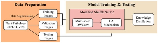
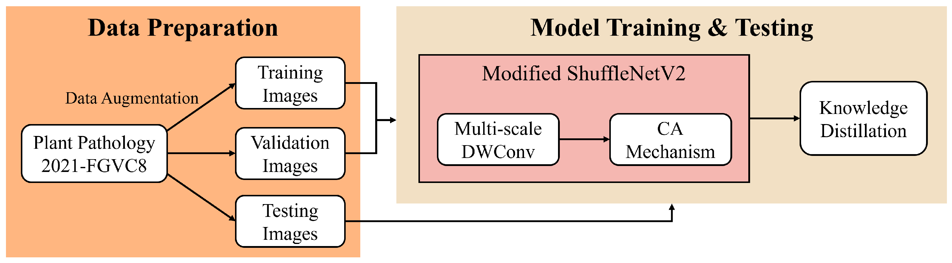
This paper tackles the challenge of accurately identifying apple leaf diseases on resource-constrained devices. The overall research workflow is illustrated in Figure 1. As depicted, the workflow consists of two main components: data preparation and model training and testing.

Figure 1. Methodology workflow of the plant leaf disease recognition model based on modified ShuffleNetV2 and knowledge distillation.

During the data preparation phase, we selected the publicly available Plant Pathology 2021-FGVC8 dataset for segmentation. The original images were first resized to match the model’s input requirements. Subsequently, the dataset was divided into training, validation, and testing sets, which were used for model training, hyperparameter tuning, and final performance evaluation, respectively. To enhance the model’s generalization ability, data augmentation techniques are dynamically applied to the training images throughout the training process.

Given the complexity of plant disease identification, directly applying the original ShuffleNetV2 poses challenges such as limited perception of multi-scale disease symptoms and vulnerability to background noise in leaf images. Therefore, in model development and training, we selected the lightweight ShuffleNetV2 0.5× network, optimized for mobile devices, as the backbone to meet the efficiency demands of edge computing. This network offers a favorable balance between computational efficiency and performance. To improve its feature extraction capabilities, we propose enhancements to ShuffleNetV2 0.5×. First, we introduce a multi-scale depthwise convolution (MDC) module (labeled “Multi-scale DWConv” in Figure 1) to handle the varying sizes of plant leaf lesions. Next, we integrate a coordinate attention (CA) mechanism (labeled “CA Mechanism” in Figure 1) to enhance the model’s focus on critical lesion regions. Despite these improvements, the inherent limitations of lightweight models may still result in performance gaps compared to larger models. To bridge this gap without increasing inference costs, we employ knowledge distillation (labeled “Knowledge Distillation” in Figure 1), where a pre-trained, more powerful teacher model guides the training of the lightweight student model.

2.1. ShuffleNetV2

In practical smart agriculture applications, models must be deployed on mobile devices or embedded systems, which have far less computational power and storage capacity compared to server-side platforms. While high-performance models like Vision Transformers deliver excellent recognition accuracy, their large parameter sizes and computational demands make real-time operation on field devices impractical. Therefore, this paper selects ShuffleNetV2 0.5×—the smallest variant in the ShuffleNetV2 family—as the foundational architecture for mobile device deployment. This lightweight network strikes an ideal balance between efficiency and performance, making it well suited for resource-constrained environments typical in agricultural settings.

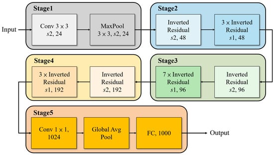
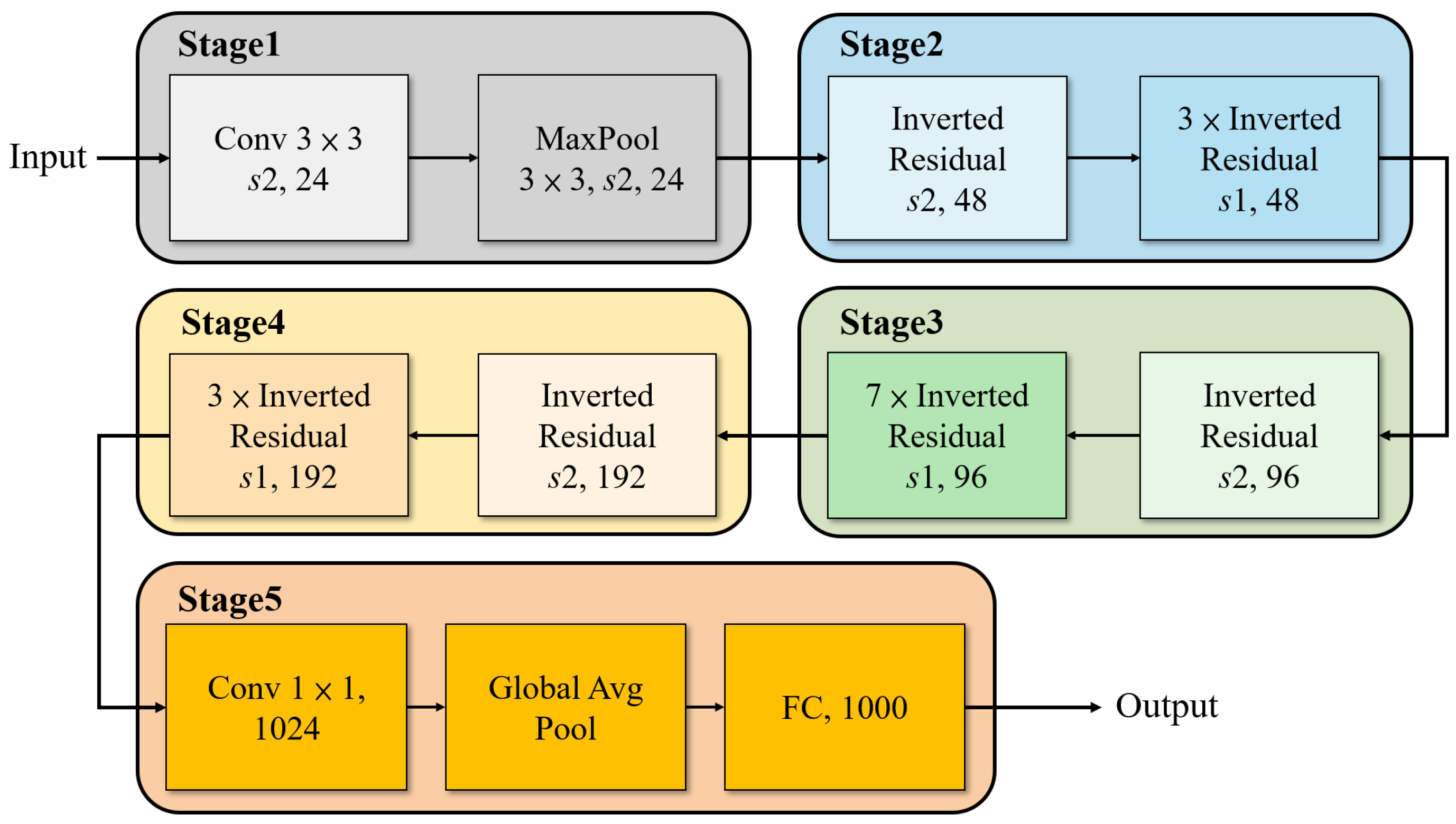
ShuffleNetV2 [20] employs a channel split mechanism that divides the input feature map into two parallel branches. One branch functions as a shortcut connection, preserving the original information to facilitate gradient propagation and efficient information flow. The other branch performs feature extraction and learning tasks. To enable effective communication between these two independent branches, a channel shuffle operation fuses cross-channel information by rearranging channels. This design significantly reduces computational complexity while maintaining high accuracy. Figure 2 illustrates the detailed network architecture, where the Inverted Residual unit serves as the fundamental building block for Stages 2 through 4. This unit implements the channel split and feature learning operations. In the operator field, “$s2$” denotes a stride of 2, applied at the start of each stage to downsample the spatial dimensions by half, while “$s1$” indicates a stride of 1, preserving spatial dimensions during feature processing.

Figure 2. Detailed architecture diagram of the ShuffleNetV2 0.5× deep learning model.

2.2. Modified ShuffleNetV2

Although ShuffleNetV2 exhibits excellent computational efficiency, its original design was primarily targeted at general image classification tasks. When applied directly to complex plant disease identification, two major challenges arise. First, the use of fixed-size convolution kernels limits the model’s ability to extract features from disease symptoms that vary widely in size. Second, the absence of an attention mechanism reduces the model’s capacity to effectively focus on critical lesion areas amidst noisy real-world backgrounds, such as foliage, soil, and lighting variations, thereby limiting classification accuracy. To overcome these issues, we introduced two key enhancements to ShuffleNetV2’s core unit: a multi-scale feature extraction module and a coordinate attention mechanism. These improvements enhance the model’s ability to detect diverse disease symptoms and accurately localize critical lesion regions. We believe that addressing these critical bottlenecks, even at the expense of a slight increase in computational overhead, is essential for optimizing overall performance and efficiency.

2.2.1. Multi-Scale Feature Extraction Module

To address the issue of incomplete feature extraction caused by fixed-size convolutional kernels in the original ShuffleNetV2—particularly when processing plant disease symptoms of varying scales in real-world environments—we designed a multi-scale depthwise convolution (MDC) module and integrated it into the existing model architecture.

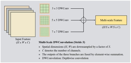
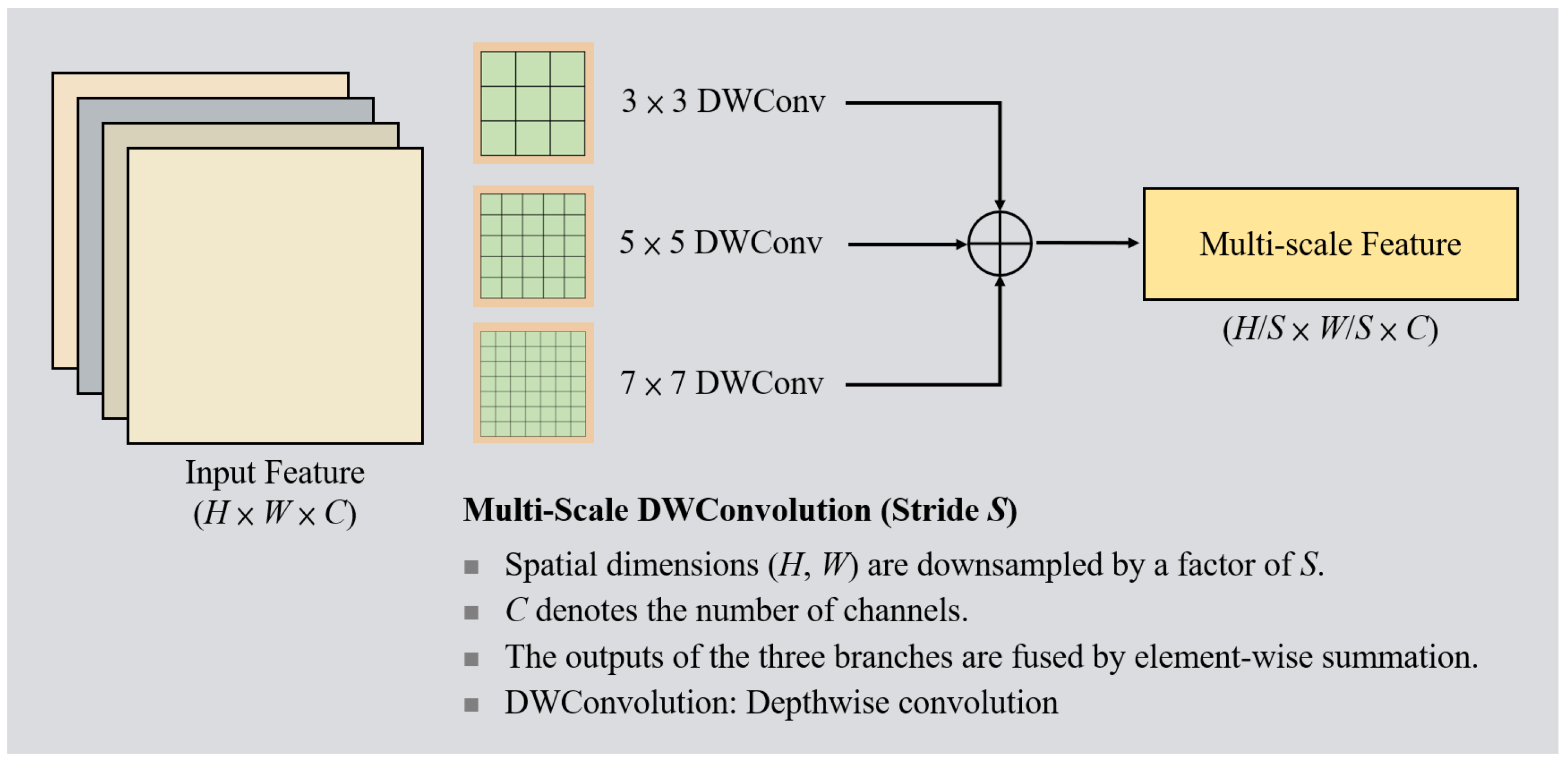
The MDC module consists of three parallel depthwise separable convolution branches with kernel sizes of $3\times 3$, $5\times 5$, and $7\times 7$. Its key feature lies in simultaneously processing feature information at multiple scales, with the outputs fused through element-wise addition to produce feature maps enriched with multi-scale information. To maintain the lightweight design principles of the original ShuffleNetV2, we applied this module selectively rather than universally across all convolutional layers. Specifically, the MDC module is deployed exclusively within Stage 2 of the ShuffleNetV2 architecture, including the initial downsampling unit (stride $=2$) and the subsequent basic units (stride $=1$), as illustrated in Figure 3. Stage 2 feature maps retain relatively high spatial resolution ($56\times 56$), making this stage ideal for capturing fine pathological details. Moreover, enriching the feature representation early in the network provides higher quality inputs to deeper layers, thereby improving recognition performance while containing computational costs.

Figure 3. Architecture of the Multi-scale Depthwise Convolution (DWConv) module for feature extraction.

2.2.2. Coordinate Attention Module

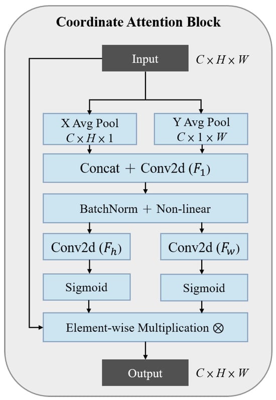
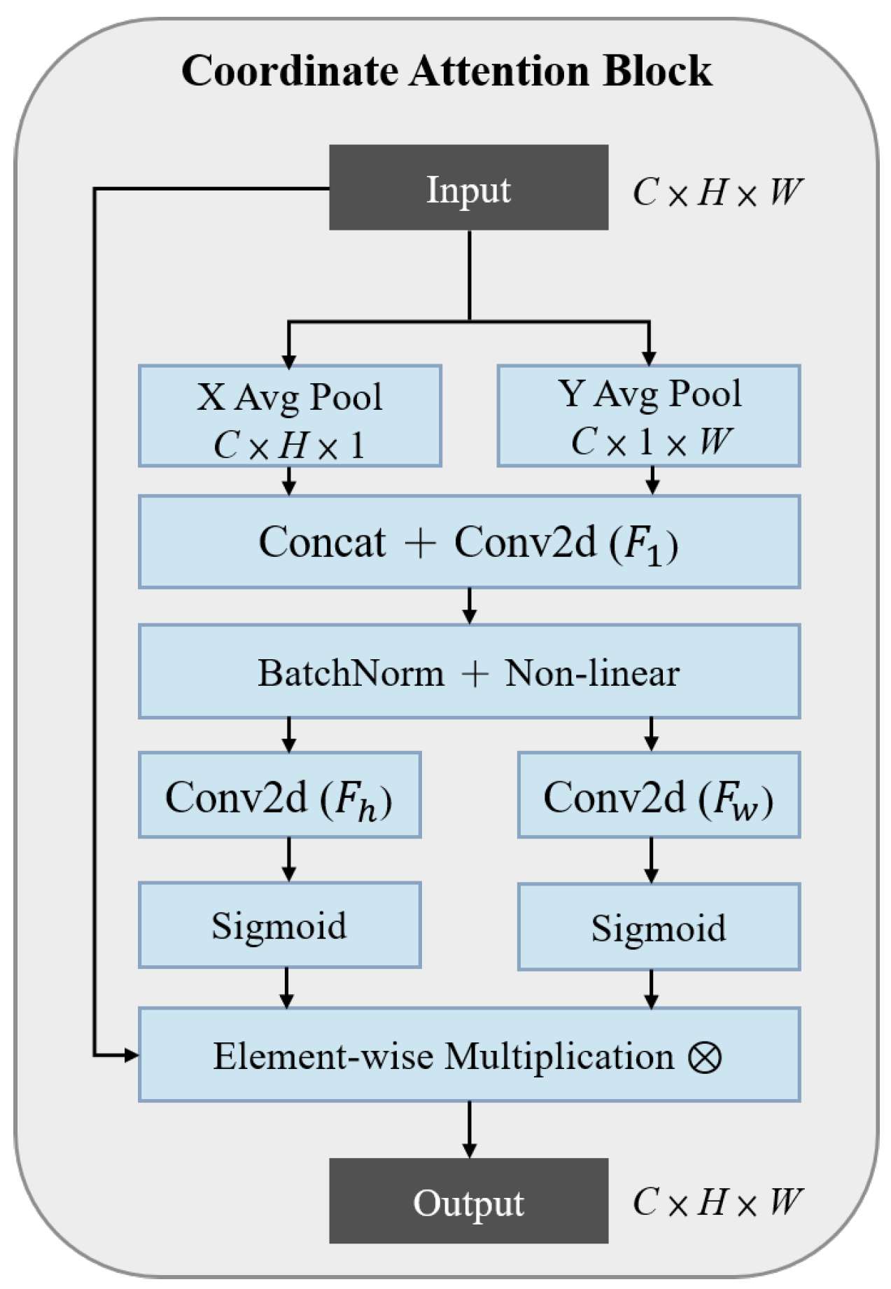
After extracting richer lesion features through the MDC module, the absence of an attention mechanism may cause important lesion features to be diluted by background noise, reducing disease classification accuracy. To address this, we introduced a coordinate attention (CA) mechanism [21] following the multi-scale convolutional module. The CA module helps the model focus its limited computational resources on the most distinguishable lesion regions. The architecture of the CA mechanism is illustrated in Figure 4.

Figure 4. Architecture of the coordinate attention (CA) module based on directional feature encoding.

The CA module embeds positional information into channel attention to enhance feature representation. To avoid spatial information loss caused by traditional two-dimensional global pooling, CA decomposes the input feature map $x_c$ into two separate one-dimensional feature encodings. Specifically, it performs one-dimensional average pooling along the width (W) and height (H) dimensions for each channel (c), producing height-wise ($z_c^h$) and width-wise ($z_c^w$) feature representations that capture spatial relationships in both vertical and horizontal directions. In Figure 4, “X Avg Pool” and “Y Avg Pool” denote the aggregation of feature information across all channels (C) along their respective spatial dimensions, resulting in two direction-aware feature tensors ($z^h$ and $z^w$). These concepts are mathematically formalized in Equations (1) and (2):

$$z_c^h\left(h\right)={\displaystyle \frac{1}{W}}\sum _{0\le w<W}{x}_c(h,w),$$

(1)

$$z_c^w\left(w\right)={\displaystyle \frac{1}{H}}\sum _{0\le h<H}{x}_c(h,w),$$

(2)

where $z_c^h$ and $z_c^w$ represent the one-dimensional feature values obtained at height h and width w along channel c, respectively.

After this step, to enable effective feature information exchange between the two directions, we perform feature fusion by sequentially applying convolution, batch normalization (BN), and an activation function to the one-dimensional features $z^h$ and $z^w$. The concept is shown in Equation (3):

$$\mathit{f}=\delta \left(\mathrm{BN}\left({\mathit{F}}_1\left([z^h,z^w]\right)\right)\right),$$

(3)

where $\mathit{f}$ represents the intermediate feature map obtained by encoding the x and y coordinate features. A $1\times 1$ convolution function $F_1$ is applied to learn correlations between the two spatial dimensions while reducing the number of channels, thereby lowering computational complexity. The Swish activation function ($\delta$) is then applied. Since this feature map (f) already contains global and cross-dimensional information, splitting it back into separate spatial dimensions generates independent attention maps for height and width ($f^h$ and $f^w$). The convolution functions ($F_h$ and $F_w$), combined with the activation function ($\sigma$), then produce two attention weights ($g^h$ and $g^w$) that capture the spatial dependencies and positional importance of features along the height and width dimensions. These weights are used to reweight the original feature map in subsequent processing. Relevant concepts are shown in Equations (4) and (5):

$$g^h=\sigma \left(F_h\left(f^h\right)\right),$$

(4)

$$g^w=\sigma \left(F_w\left(f^w\right)\right).$$

(5)

Finally, the computed height and width attention weights ($g^h$ and $g^w$) are expanded and multiplied element-wise with the original input feature map ($x_c$), producing the weighted output feature map ($y_c$), as shown in Equation (6):

$$y_c(h,w)=x_c(h,w)\times g_c^h\left(h\right)\times g_c^w\left(w\right),$$

(6)

where $x_c(h,w)$ denotes the value of the c channel in the input feature map at coordinates $(h,w)$, while $y_c(h,w)$ represents the corresponding output value. Additionally, $g_c^h\left(h\right)$ represents the weight value in the c channel and h column of the height attention weight $g^h$, while $g_c^w\left(w\right)$ denotes the weight value in the c channel and w row of the width attention weight $g^w$. This operation enables the model to autonomously enhance features in critical regions based on learned spatial importance while suppressing features in non-critical areas.

2.2.3. ShuffleNetV2 Core Unit Modification

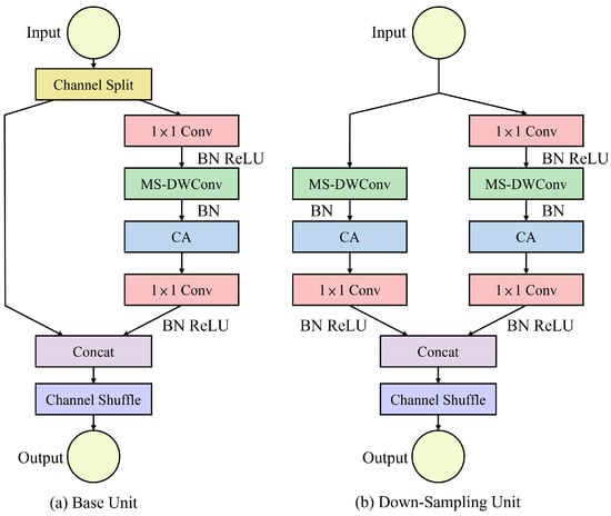
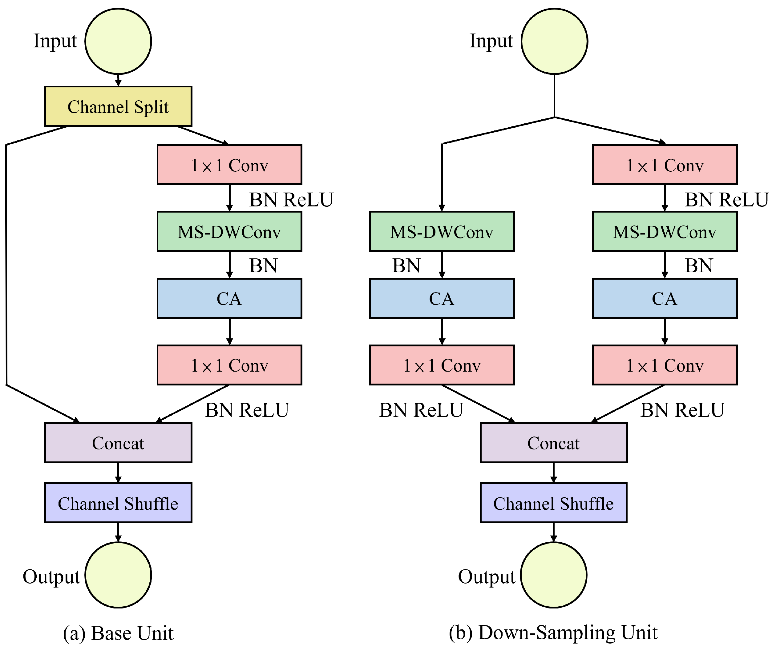
After integrating the multi-scale feature extraction module with the coordinate attention mechanism, we designed two modified ShuffleNetV2 core units: a base unit and a downsampling unit. Their detailed architectures are illustrated in Figure 5. Taking the base unit (Figure 5a) as an example, when a set of feature maps enters this unit, it is first split into two parts. One half of the channels retains the original information and proceeds directly to the subsequent fusion stage, ensuring stable gradient propagation. The other branch enters the feature processing path, where the feature map undergoes sequential $1\times 1$ convolutions to expand the number of channels. Next, the MDC module captures spatial features of lesions at different scales. Following this, the CA module filters and weights these features, focusing on regions with high discriminative power. Finally, the two feature streams are fused through concatenation (Concat) and channel shuffling (Channel Shuffle). This design preserves ShuffleNetV2’s high efficiency while enhancing its ability to perceive multi-scale targets and localize critical regions.

Figure 5. Architecture of the modified ShuffleNet unit based on multi-scale depthwise convolution and coordinate attention: (a) base unit and (b) down-sampling unit.

The downsampling unit shown in Figure 5b is deployed at the beginning of Stage 2. Unlike the base unit, this unit performs stride-2 MS-DWConv operations on both the left and right branches to achieve downsampling, significantly reducing the spatial dimensions. A subsequent $1\times 1$ convolution then adjusts the number of channels to facilitate feature fusion, effectively halving the spatial dimensions at the output.

2.3. Knowledge Distillation

Although we have enhanced the ShuffleNetV2 architecture with multi-scale feature extraction and coordinate attention mechanisms to better adapt it for apple leaf disease identification, its feature representation capacity remains limited due to its lightweight design and reduced channel count. As a result, it exhibits accuracy gaps compared to larger models, especially when identifying complex disease symptoms. To close this performance gap without increasing inference costs, we employ knowledge distillation [22].

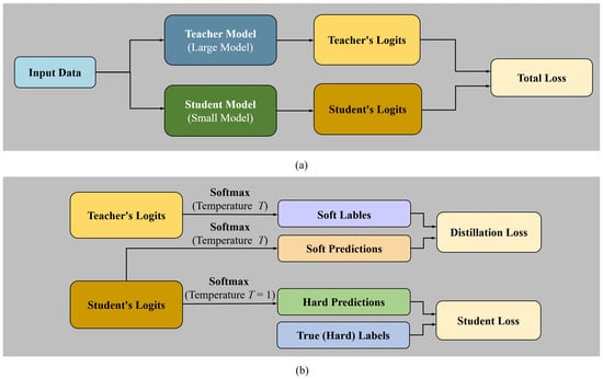
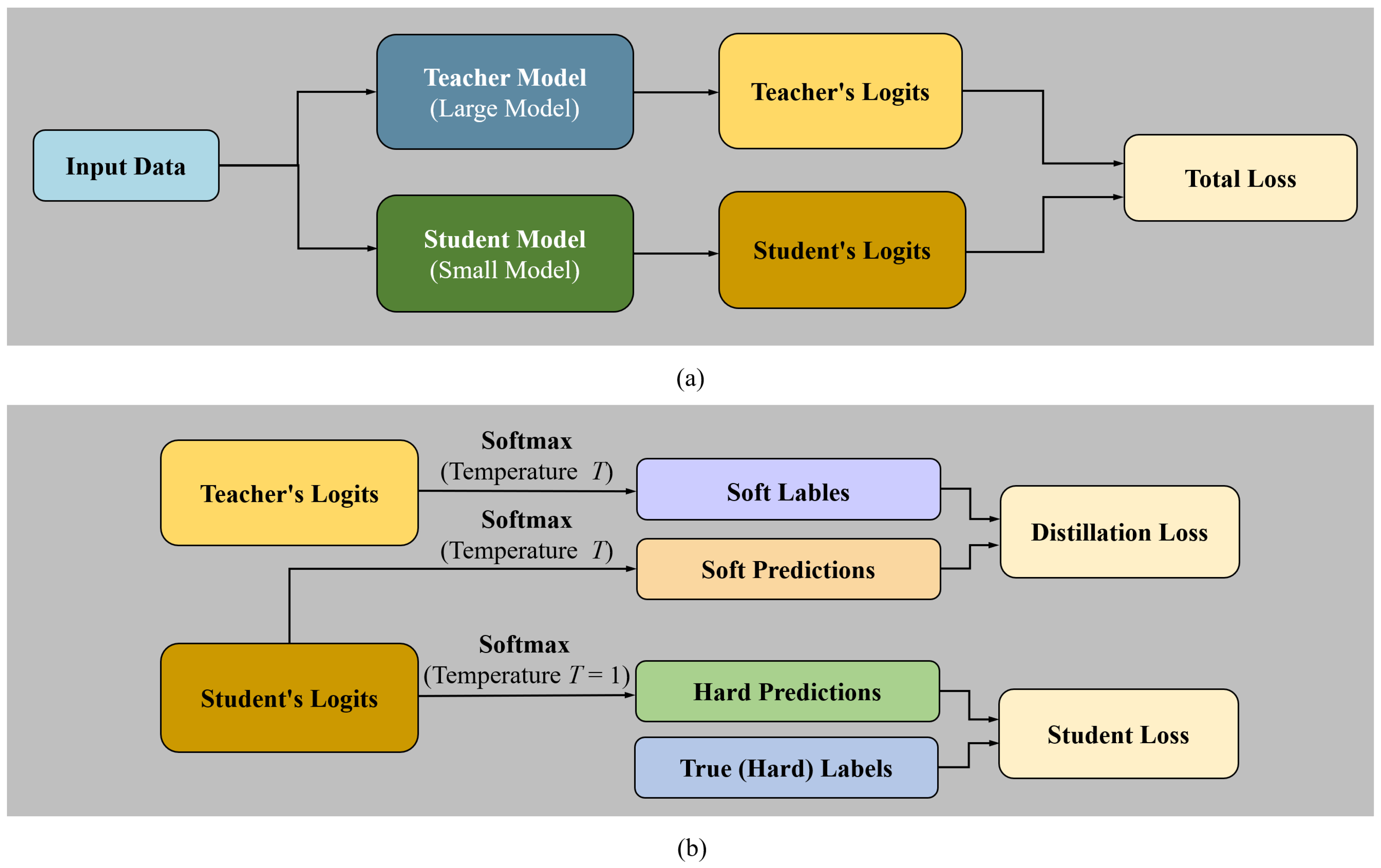
Knowledge distillation is an effective model compression and knowledge transfer technique that uses a fully trained, structurally complex, high-performance teacher model to guide the training of a smaller, simpler student model with fewer parameters. By aligning the student model’s outputs with the probability distribution of the teacher model’s outputs, the student learns to replicate the teacher’s mapping from input data to output labels, thereby improving its classification performance. Given ResNet50’s outstanding performance across multiple visual tasks and this dataset [23,24], we select the pre-trained ResNet50 as the teacher model in this study. The training process for knowledge distillation is illustrated in Figure 6.

Figure 6. Knowledge distillation training framework and loss function calculation flow for small model training: (a) teacher–student model overview, and (b) detailed softmax loss calculation based on temperature.

During the knowledge distillation training phase, the student model’s learning objective consists of two weighted loss functions. The first is the traditional supervised loss $L_{Student}$, referred to as the “Student Loss” in Figure 6b, which ensures the student learns to fit the true labels (hard labels). This loss is computed using the standard cross-entropy function to measure the difference between the student model’s predictions $\sigma \left(z_s\right)$—processed through the Softmax function ($\sigma$)—and the true label $T_b$, as shown in Equation (7):

$$L_{Student}=\mathrm{CrossEntropy}(T_b,\sigma \left(z_s\right)).$$

(7)

The second component is the distillation loss $L_{Distillation}$, shown as the “Distillation Loss” in Figure 6b. Its purpose is to align the student model’s output probability distribution with that of the teacher model. To help the student learn the intrinsic relationships between categories, rather than just the correct labels, a temperature parameter (Temperature, $T>1$) is introduced. By dividing the logits of both the teacher and student models (denoted as $z_t$ and $z_s$, respectively) by this temperature (T) before applying the Softmax function, a smoother probability distribution—called the soft labels—is obtained. These soft labels capture the similarity between different classes as perceived by the teacher. Higher values of T amplify the probabilities of incorrect classes, guiding the student to pay attention to which misclassifications the teacher considers more likely. This enriches the student’s understanding of the class structure. The distillation loss is computed using the Kullback–Leibler (KL) divergence between the softened outputs of the student ($\sigma (z_s/T)$) and teacher ($\sigma (z_t/T)$) models, as shown in Equation (8):

$$L_{Distillation}=T^2\times \mathrm{KL}(\sigma (z_s/T),\sigma (z_t/T)),$$

(8)

where the correction coefficient $T^2$ ensures that the gradient magnitude remains relatively stable as the temperature T varies. Ultimately, the total loss function $L_{total}$ is formed by a weighted combination of the supervised loss and the distillation loss, as shown in Equation (9):

$$L_{total}=\alpha ·L_{Distillation}+(1-\alpha )·L_{Student}.$$

(9)

The hyperparameter $\alpha$ balances the weighting between learning from true labels and soft labels in the student model. By minimizing this combined loss function, the student model learns both to fit the true data and to emulate the teacher model’s decision logic and class relationships. In practical smart agriculture applications, knowledge distillation effectively improves recognition accuracy while maintaining the lightweight nature of the model. Our goal is to distill the superior recognition capabilities of the ResNet50 teacher model into our modified lightweight ShuffleNetV2 student model.

3. Experimental Results

3.1. Experimental Environment

Our experimental setup includes an 8-core computer powered by an Intel Core i7-10700 CPU, an NVIDIA GeForce RTX 3080 GPU, and 16 GB of RAM. The system runs Windows 11 Professional as the operating system. The development environment is built on Anaconda version 23.7.4 with Python 3.12.11, utilizing the PyTorch 2.7.1 deep learning framework along with CUDA 12.8 and cuDNN 9.7.1 GPU drivers.

3.2. Experimental Datasets

To verify the effectiveness of the proposed model and its generalization capability across different environments, this study utilizes two large-scale apple leaf disease datasets: Plant Pathology 2021-FGVC8 and AppleLeaf9.

3.2.1. Plant Pathology 2021-FGVC8 Dataset

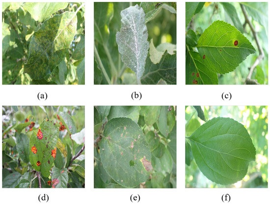
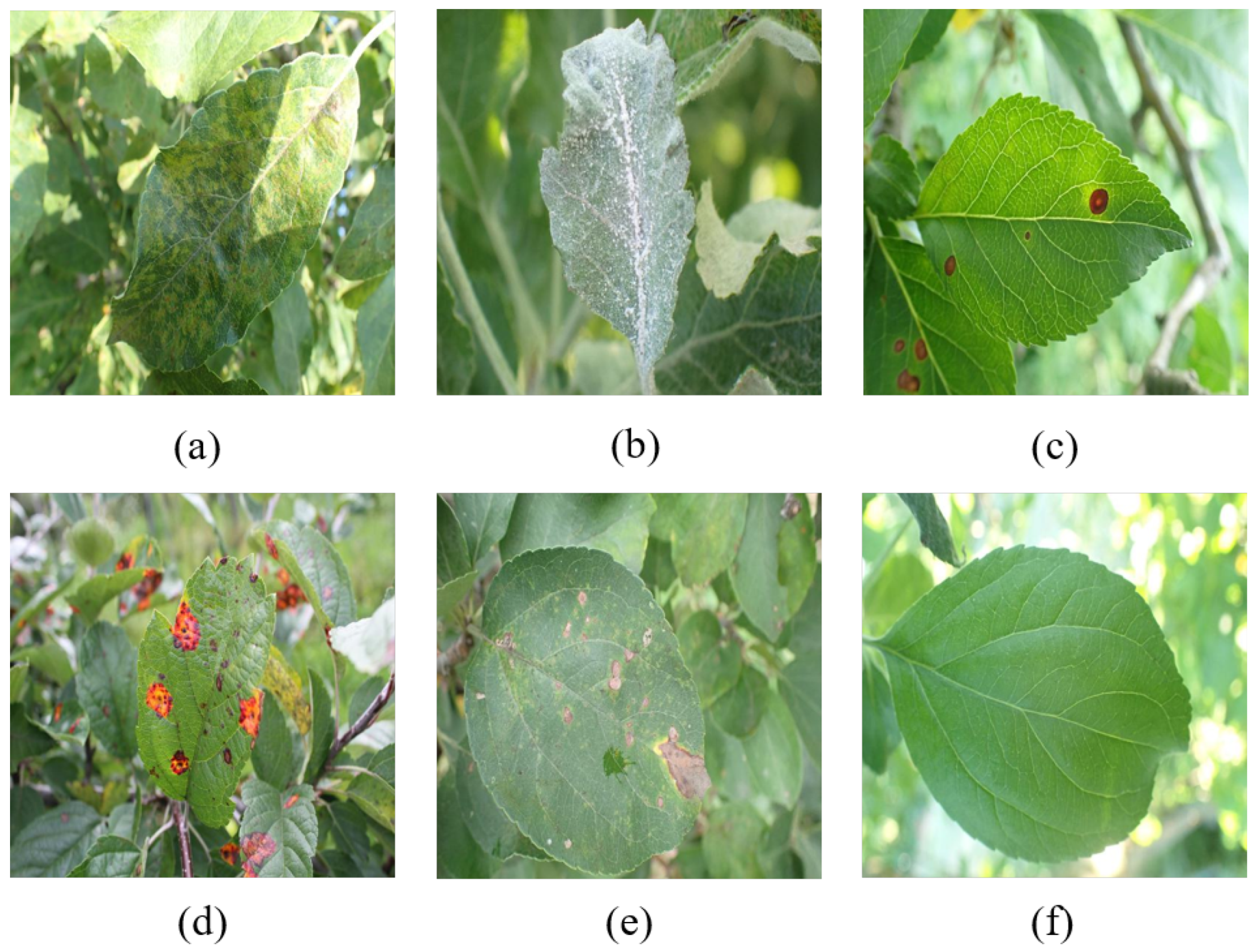
This paper uses the Plant Pathology 2021-FGVC8 dataset [25], which was provided by the Fine-Grained Visual Categorization competition held at CVPR 2021 and is publicly accessible on the Kaggle platform. The dataset consists of 18,632 high-quality RGB images of apple leaves captured under natural agricultural conditions. It represents diverse lighting, backgrounds, and leaf maturity stages, reflecting real-world field scenarios. All images are expert-annotated into six classes: scab, powdery mildew, frog eye leaf spot, rust, complex disease, and healthy. The “complex” category denotes leaves exhibiting multiple symptoms simultaneously, a common occurrence in actual field environments that adds to classification complexity. Sample images from the dataset are displayed in Figure 7.

Figure 7. Sample apple leaf images from the Plant Pathology 2021-FGVC8 dataset: (a) scab, (b) powdery mildew, (c) frog eye leaf spot, (d) rust, (e) complex, and (f) healthy.

3.2.2. AppleLeaf9 Dataset

To further validate the stability and generalization capability of the proposed model across different sampling environments, this study introduces the AppleLeaf9 public dataset [26]. This dataset addresses the challenges of identifying apple leaf diseases in real-world field environments. AppleLeaf9 integrates data from PVD, PPCD2020, and other sources, containing images of single leaves, complex backgrounds, and multiple disease symptoms, making it highly challenging and representative. Table 1 presents the data distribution for each category in this dataset.

Table 1. Class-wise image counts and data splits in the AppleLeaf9 dataset.

Types	Image Number	Training Img.	Validation Img.	Testing Img.
Alternaria leaf spot	417	292	42	83
Brown spot	411	288	41	82
Frog eye leaf spot	3181	2227	318	636
Grey spot	339	238	34	67
Health	516	362	51	103
Mosaic	371	260	37	74
Powdery mildew	1184	829	119	236
Rust	2753	1928	275	550
Scab	5410	3787	541	1082
Total	14,582	10,211	1458	2913

3.3. Experimental Setup

3.3.1. Image Preprocessing and Data Augmentation

Due to the high resolution (e.g., 4000 × 2672 pixels) and variable dimensions of the original images in the Plant Pathology 2021-FGVC8 dataset, performing dynamic resizing on-the-fly for each training batch can lead to I/O bottlenecks and unnecessary computational overhead. To improve data loading efficiency and speed up model training, all images were uniformly resized to 384 × 384 pixels prior to training. The dataset was then randomly divided into training, validation, and test sets with a 7:1:2 ratio to ensure robust training, validation, and performance evaluation. The sample counts for each category are summarized in Table 2.

Table 2. Class-wise image counts and data splits in the Plant Pathology 2021-FGVC8 dataset.

Types	Image Number	Training Img.	Validation Img.	Testing Img.
Complex	2957	2070	296	591
Frog eye leaf spot	3181	2227	318	636
Healthy	4624	3237	463	924
Powdery mildew	1184	829	119	236
Rust	1860	1302	186	372
Scab	4826	3379	482	965
Total	18,632	13,044	1864	3724

To further increase the diversity of training data and reduce model overfitting, we applied RandAugment [27] data augmentation to the training set. RandAugment simplifies augmentation by randomly selecting a fixed number of transformations—such as rotation, color adjustment, translation, and autocontrast—from a predefined list and applying them sequentially to each input image. This process generates a wide variety of altered training samples, enhancing data variability. By exposing the model to diverse synthetic disturbances, RandAugment improves the model’s generalization and robustness to real-world variations like lighting changes and different viewing angles.

3.3.2. Training Parameter Setting

Given the variation in complexity and convergence behaviors across different model architectures, we employed the ReduceLROnPlateau learning rate scheduler with adaptive adjustment in all experiments to promote stable convergence during later training stages. This strategy monitors the validation loss and automatically reduces the learning rate when the loss metric plateaus for a predefined number of consecutive epochs (patience). By doing so, it helps accelerate convergence by allowing finer optimization steps once improvement stagnates, thereby improving training stability and final model performance.

To ensure fair comparison across different lightweight models and maintain experimental consistency, independent hyperparameter tuning for each model was not performed. Instead, we adopted widely used hyperparameter settings common in lightweight CNN research, with specific configurations detailed in Table 3. For the multi-class classification task addressed, we used the standard cross-entropy loss function as the training objective. The AdamW optimizer was selected due to its ability to provide more stable convergence for CNN architectures compared to traditional optimizers like SGD or Adam.

Table 3. The various hyperparameter setting used in the proposed approach.

Hyperparameter	Value/Method
Initial Learning Rate	$1\times {10}^{-3}$
Batch Size	64
Max Epochs	150
Optimizer	AdamW
LR Scheduler	ReduceLROnPlateau
LR Scheduler Patience	7
LR Reduction Factor	0.1
Early Stopping Patience	15
Loss Function	Cross-Entropy

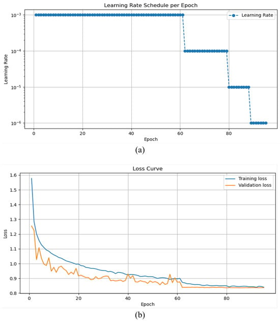
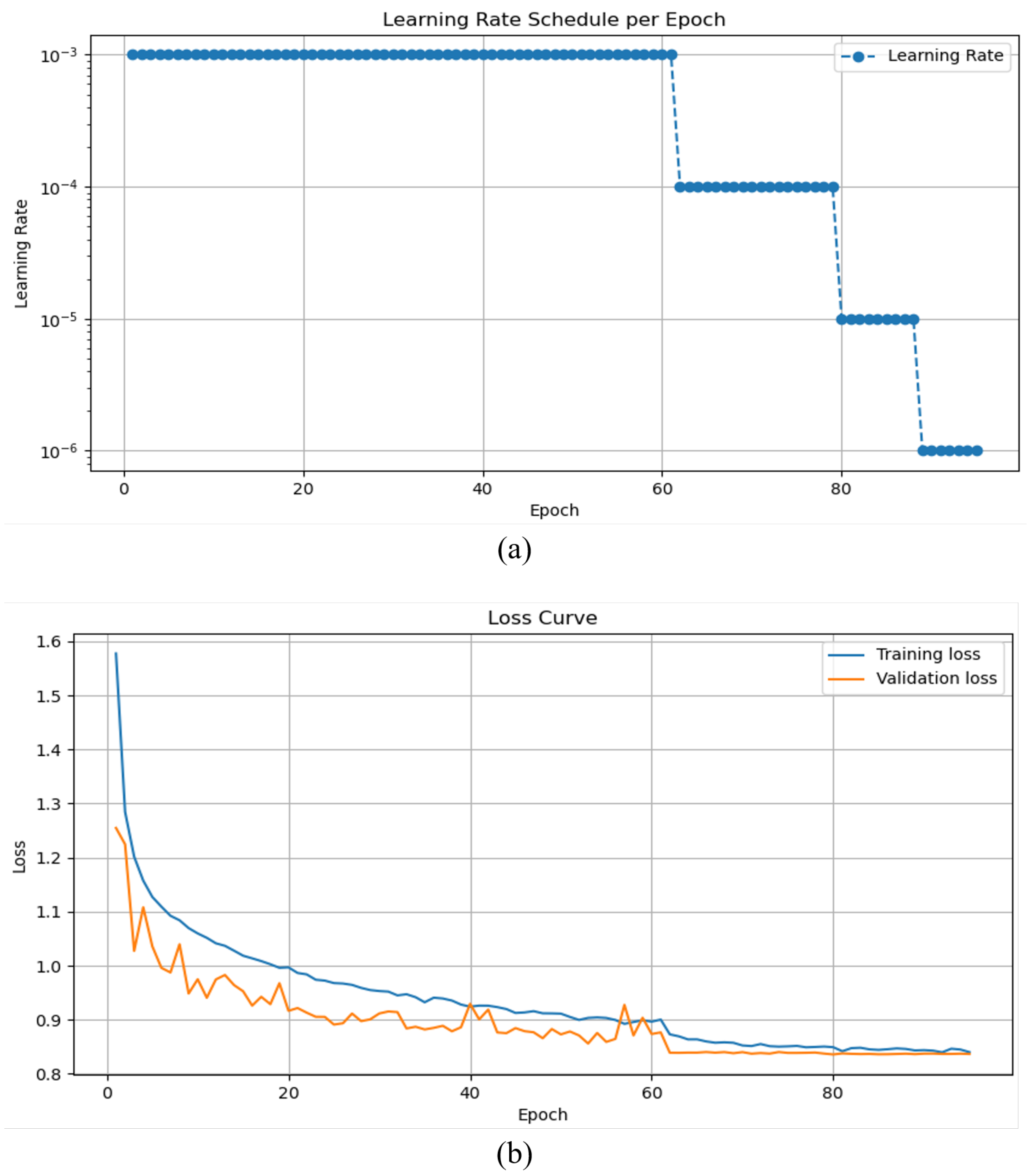
During the knowledge distillation phase, the training objective differs from learning from scratch. At this stage, the student model no longer explores an entirely new weight space but instead undergoes fine-tuning guided by a pre-trained teacher model. Consequently, a smaller learning rate is required during distillation compared to the initial training phase to ensure stable fine-tuning. To justify this, we analyzed the learning rate schedule during the student model’s initial training, as shown in Figure 8. The student model began with an initial learning rate alongside the ReduceLROnPlateau strategy (patience = 7). When the learning rate decreased at epoch 62, validation loss improved. However, early stopping with patience set to 15 was only triggered at epoch 95 during the late training phase, by which point the learning rate had dropped further. This suggests that learning rates below this threshold may lack sufficient momentum to make meaningful parameter updates or escape local minima.

Figure 8. The effect of learning rate schedule on student model convergence: (a) adaptive learning rate schedule via ReduceLROnPlateau and (b) corresponding training and validation loss curves.

We ultimately selected an initial learning rate for the knowledge distillation phase that balances between the higher learning rate used during the student model’s initial training and the lower learning rate observed when the model’s performance begins to plateau. This choice ensures stable fine-tuning while retaining sufficient momentum for effective exploration and convergence toward an optimal parameter space under the teacher model’s guidance. Aside from this adjustment to the learning rate, all other hyperparameters remain consistent with those used during the initial training phase to maintain experimental control over variability.

3.4. Experimental Results and Analysis

This section presents a series of experiments designed to validate the effectiveness of our proposed method, along with analysis of the results.

• Experiment 1 establishes the baseline model’s performance as a foundation for subsequent improvement comparisons.
• Experiment 2 conducts ablation studies to individually verify the contributions of the MDC module, CA attention mechanism, and knowledge distillation to overall model performance.
• Experiment 3 evaluates the rationale for selecting the CA module by comparing its performance against several mainstream attention mechanisms.
• Experiment 4 analyzes the impact of knowledge distillation hyperparameters (temperature (T) and weight ($\alpha$)) to identify the optimal parameter combinations.
• Experiments 5 and 6 compare our proposed model against other leading lightweight models and relevant literature to assess its competitiveness in terms of accuracy and efficiency.

To quantitatively evaluate model performance, this paper employs accuracy, precision, recall, and F1-score as the primary evaluation metrics, with their calculation formulas presented in Equations (10)–(13):

$$Accuracy={\displaystyle \frac{TP+TN}{TP+TN+FP+FN}},$$

(10)

$$Precision={\displaystyle \frac{TP}{TP+FP}},$$

(11)

$$Recall={\displaystyle \frac{TP}{TP+FN}},$$

(12)

$$F1-score={\displaystyle \frac{2\times Precision\times Recall}{Precision+Recall}}.$$

(13)

Among the evaluation metrics mentioned, True Positive (TP) means an actual positive sample is correctly predicted as positive, False Positive (FP) means an actual negative sample is incorrectly predicted as positive, False Negative (FN) means an actual positive sample is incorrectly predicted as negative, and True Negative (TN) means an actual negative sample is correctly predicted as negative. Additionally, we compare models based on their parameter counts and computational complexity, measured in Floating Point Operations (FLOPs), to assess efficiency alongside predictive performance.

3.4.1. Baseline Model Performance

First, we established the baseline model using ShuffleNetV2 0.5×. Without pre-trained weights or data augmentation, this lightweight model achieved an accuracy of only 88.08%. Incorporating ImageNet pre-trained weights improved the accuracy to 90.12%, demonstrating the benefits of transfer learning. Further applying RandAugment data augmentation raised the accuracy to 90.84%, indicating that this augmentation strategy effectively enhances the model’s generalization ability.

To simplify the presentation of subsequent experimental data, this study refers to the original ShuffleNetV2 0.5× model as SN-Base, the version with pre-trained weights as SN-TL (Transfer Learning), and the model additionally incorporating data augmentation as SN-DA (Data Augmentation). Since SN-DA demonstrates superior performance, it serves as the baseline for comparisons in the subsequent experiments. Additional relevant performance metrics are presented in Table 4.

Table 4. Effect of transfer learning and data augmentation on ShuffleNet-based model performance.

Model	Accuracy (%)	Precision (%)	Recall (%)	F1-Score (%)
SN-Base	88.08	86.91	87.03	86.87
SN-TL	90.12	88.84	89.11	88.87
SN-DA (Baseline)	90.84	89.74	89.97	89.65

3.4.2. Ablation Study

To validate the specific contributions of each modified module in this study, we conducted ablation experiments by progressively adding the MDC module, CA module, and knowledge distillation (KD) strategy on top of the baseline model. The results of these experiments are presented in Table 5.

Table 5. Performance Contribution of Integrated Components.

Architecture	Acc. (%)	Pre. (%)	Rec. (%)	F1-Score (%)	Params (M)	FLOPs (G)
Baseline	90.84	89.74	89.97	89.65	0.3479	0.0789
Baseline + MDC	91.43	90.42	90.33	90.29	0.3568	0.0929
Baseline + CA	91.92	90.87	90.96	90.91	0.3512	0.0792
Baseline + KD	92.29	90.92	91.56	91.18	0.3479	0.0789
Baseline + MDC + CA	92.64	91.48	91.52	91.45	0.3601	0.0931
Baseline + MDC + KD	92.37	91.10	91.37	91.20	0.3568	0.0929
Baseline + CA + KD	92.88	91.76	92.23	91.82	0.3512	0.0792
Baseline + MDC + CA + KD (Ours)	93.15	91.95	92.20	92.04	0.3601	0.0931

First, the MDC module was integrated into Stage 2 of the baseline model. Experimental results show that adding the MDC module increases the model’s accuracy to 91.43%. This demonstrates that the MDC module enhances the model’s ability to capture features at multiple spatial scales, thereby improving recognition performance.

Subsequently, building on the integration of the MDC module, we incorporated the CA module. Experimental results show that adding the CA module increased accuracy to 92.64%, demonstrating its effectiveness in enhancing feature selection and weighting. The CA module guides the model’s attention toward diagnostically important regions, thereby minimizing the impact of background noise and irrelevant factors.

Finally, knowledge distillation (KD) was applied to the model integrating MDC and CA (Baseline + MDC + CA) to enhance the recognition performance and generalization of the lightweight student model. Experimental results show that accuracy increased to 93.15%, along with improvements in Precision, Recall, and F1-Score. These findings demonstrate that knowledge distillation is an effective optimization technique for improving the performance of lightweight student models.

Furthermore, the comprehensive ablation study comprising eight experimental configurations, as shown in Table 5, reveals the synergistic effects between the modules. The results indicate that while individual modules provide incremental gains, their combination achieves a higher performance ceiling. Notably, the introduction of knowledge distillation significantly improves accuracy without increasing inference latency, demonstrating that transferring knowledge from a high-capacity teacher model is crucial for enabling the lightweight model to capture subtle pathological features.

3.4.3. Comparative Analysis of Attention Mechanisms

To validate the performance of the CA module, we conducted a comparative analysis with four other mainstream attention mechanisms: CBAM [28], ECA [29], SA (Shuffle Attention) [30], and MCA (Multidimensional Collaborative Attention) [31]. All these attention modules were trained and evaluated within the Baseline + MDC (B-MDC) architecture. Relevant experimental results are summarized in Table 6.

Table 6. Performance comparison of B-MDC with various attention modules.

Attention Module	Acc. (%)	Pre. (%)	Rec. (%)	F1-Score (%)	Params (M)	FLOPs (G)
B-MDC	91.43	90.42	90.33	90.29	0.3568	0.0929
B-MDC + CBAM	92.53	91.45	91.55	91.46	0.3626	0.0936
B-MDC + ECA	92.27	91.22	91.40	91.23	0.3568	0.0930
B-MDC + SA	92.00	91.09	91.14	91.02	0.3570	0.0930
B-MDC + MCA	91.76	90.53	90.71	90.49	0.3569	0.0930
B-MDC + CA	92.64	91.48	91.52	91.45	0.3601	0.0931

Experimental results demonstrate that compared to the B-MDC model without attention mechanisms (with an accuracy of 91.43%), all tested attention modules produced varying degrees of performance improvement, clearly showcasing the effectiveness of attention mechanisms in emphasizing relevant features for plant leaf disease identification. Among them, the model with the CA module attained the highest accuracy. Moreover, compared to the computationally heavier CBAM, CA achieved better performance with only a negligible increase in computational complexity and parameter count over the B-MDC model without attention. This highlights CA’s ability to balance accuracy gains with efficiency, validating its selection as the attention mechanism in this study.

3.4.4. Hyperparameter Analysis for Knowledge Distillation

The effectiveness of knowledge distillation depends on two key hyperparameters: temperature (T) and the loss weighting coefficient ($\alpha$). To find the optimal combination, this experiment performed a grid search on the validation set, testing various values of temperature $T=\{4,8,10\}$ and weight $\alpha =\{0.3,0.5,0.7,0.9\}$. The corresponding experimental results are presented in Table 7.

Table 7. Effect of knowledge distillation hyperparameters ($\alpha$ and T) on model performance (in %).

$\mathit{\alpha }\setminus \mathit{T}$	4	8	10
0.3	92.86	93.56	93.88
0.5	93.29	93.56	93.78
0.7	93.29	93.62	93.67
0.9	93.67	93.40	92.86

Experimental data reveal a significant interaction between temperature (T) and loss weighting coefficient ($\alpha$) in knowledge distillation. When $\alpha$ is low, the model primarily relies on hard labels, and increasing T allows the model to learn richer categorical relationship information from the soft labels, resulting in performance gains. However, this trend does not always hold. At higher $\alpha$ values, increasing T can cause accuracy to decline, likely due to overly smoothed soft labels combined with high imitation weights. This may lead the student model to overfit the teacher’s output distribution while neglecting crucial information from the hard labels.

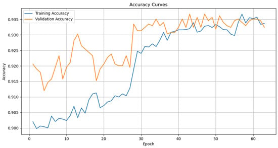
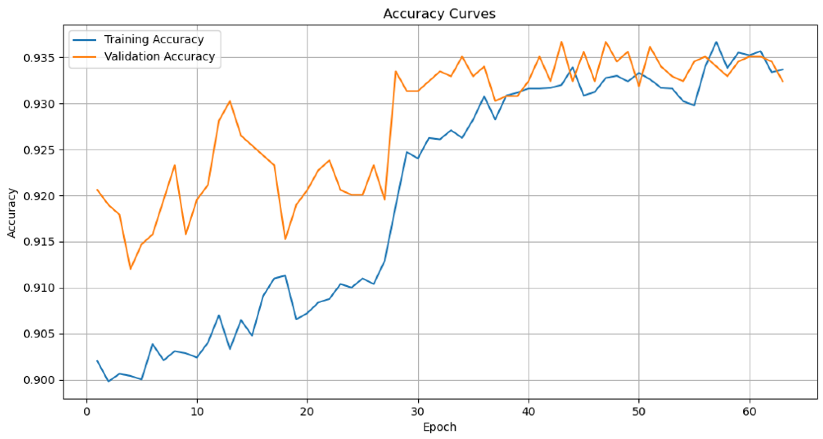
The experimental results in Table 7 show that the combination of temperature $T=10$ and weight $\alpha =0.3$ achieves the highest accuracy of 93.88% on the validation set. This setting effectively leverages the inter-class information contained in soft labels while ensuring the model fully learns accurate information from hard labels through the relatively low $\alpha$, achieving an optimal balance. Therefore, this hyperparameter configuration is adopted. Additionally, Figure 9 illustrates the accuracy trends on the training and validation sets under this configuration during knowledge distillation. The pre-trained student model started with an initial accuracy around 90.0%. Within the first 30 epochs, validation accuracy exhibited rapid growth with some fluctuations, while training accuracy increased more smoothly, reflecting the student’s learning and adaptation from the teacher. Eventually, both accuracies converged around 93.3% to 93.5%, with a narrow gap indicating minimal overfitting. Once the validation performance plateaued, early stopping triggered after 15 consecutive epochs without improvement, terminating training at epoch 63.

Figure 9. Training and validation accuracy curves of the model under knowledge distillation hyperparameters ($\alpha =0.3$ and $T=10$).

3.4.5. Performance Comparison with Other Lightweight Models

To validate the comprehensive performance and efficiency advantages of the proposed model, we compared it with several mainstream lightweight and medium-weight models. These include SqueezeNet 1.1 [32], known for its efficiency; MobileNetV4-Conv-Small [33]; GhostNetV2 1.0x [34]; various scales of ShuffleNetV2 (including the baseline 0.5× and larger 1.0× and 1.5× versions); the high-performing EfficientNetV2-B0 [35]; and the widely used ResNet series, including ResNet34d and ResNet50 as the teacher models. Relevant experimental results are summarized in Table 8.

Table 8. Performance and efficiency comparison of ’Ours’ with state-of-the-art deep learning models.

Method	Acc. (%)	Pre. (%)	Rec. (%)	F1-Score (%)	Params (M)	FLOPs (G)
ResNet34d	94.58	93.62	93.70	93.63	21.3070	7.8058
ResNet50	94.76	93.61	93.99	93.77	23.5203	8.1744
GhostNetV2 1.0	91.97	90.37	91.08	90.66	4.8836	0.3317
SqueezeNet 1.1	92.53	91.26	91.48	91.31	0.7256	0.5311
MobileNetV4-Conv-Small	88.61	87.18	87.99	87.03	2.5007	0.7514
EfficientNetV2-B0	93.56	92.53	92.72	92.61	5.8664	1.4337
ShuffleNetV2 0.5×	90.84	89.74	89.97	89.65	0.3479	0.0789
ShuffleNetV2 1.0×	93.26	91.98	91.96	91.90	1.2598	0.2878
ShuffleNetV2 1.5×	92.72	91.82	91.59	91.69	2.4848	0.5895
Ours	93.15	91.95	92.20	92.04	0.3601	0.0931

Experimental results demonstrate that the proposed method significantly outperforms most lightweight models in terms of both parameter count and computational complexity. For example, it uses approximately half the parameters of SqueezeNet 1.1 and has substantially lower computational complexity than MobileNetV4-Conv-Small and GhostNetV2 1.0. While its accuracy is slightly lower than that of EfficientNetV2-B0, it requires far fewer parameters and computational resources, showcasing remarkable computational efficiency. Compared to the larger ShuffleNetV2 1.0× model, our approach achieves only 0.11% lower accuracy but reduces parameters and computational complexity by about 71.4% and 67.7%, respectively. Interestingly, the ShuffleNetV2 1.5× model performs worse than both the 1.0× variant and our model, likely due to overfitting caused by the relatively limited dataset size compared to its model capacity. Against the teacher model ResNet50, our model uses merely 1.5% of the parameters and 1.1% of the computational cost, while narrowing the accuracy gap to 1.61%. These findings affirm that our method competes favorably with more complex models, balancing strong recognition performance and computational efficiency at very low resource consumption.

3.4.6. Generalization Analysis on the AppleLeaf9 Dataset

To verify the stability of the model in real-world scenarios, we conducted comparative experiments on the AppleLeaf9 dataset. As shown in Table 9, the improved model proposed in this study also achieved excellent performance on this dataset.

Table 9. Performance Comparison with Representative Models on AppleLeaf9 Dataset.

Method	Acc. (%)	Pre. (%)	Rec. (%)	F1-Score (%)	Params (M)	FLOPs (G)
ResNet34d	97.97	97.05	96.60	96.82	21.3085	7.8058
ResNet50	98.39	97.61	97.67	97.60	23.5265	8.1744
GhostNetV2 1.0	97.46	96.12	96.20	96.12	4.8874	0.3317
SqueezeNet 11.1	97.46	96.68	95.37	96.00	0.7271	0.5316
MobileNetV4-Conv-Small	93.17	90.94	87.81	89.20	2.5046	0.7514
EfficientNetV2-B0	98.18	97.47	96.83	97.10	5.8702	1.4337
ShuffleNetV2 0.5×	95.67	93.61	92.13	92.82	0.3510	0.0789
ShuffleNetV2 1.0×	97.80	97.16	96.78	96.97	1.2628	0.2878
ShuffleNetV2 1.5×	98.15	97.35	97.25	97.29	2.4878	0.5895
Ours	97.85	97.62	97.37	96.93	0.3631	0.0931

4. Discussion

To thoroughly examine the effectiveness of the proposed model and explore the sources of its advantages over the baseline, this section presents experimental results using confusion matrices and Grad-CAM++ visualizations for detailed discussion.

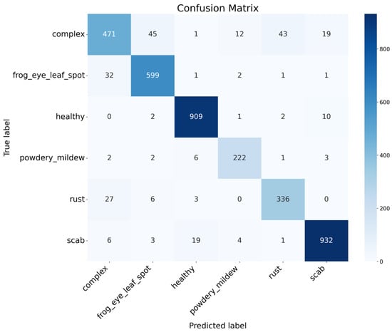
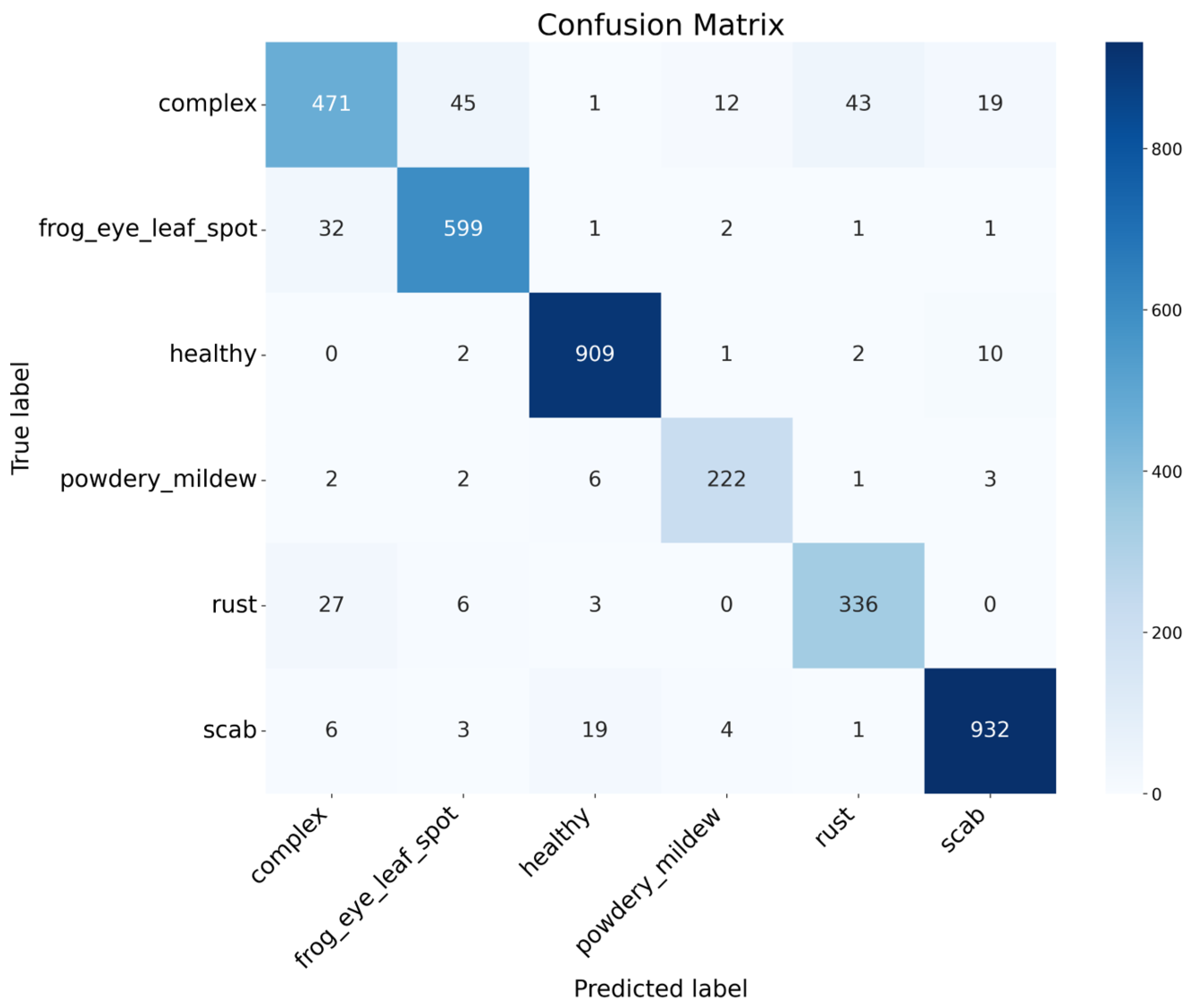
As shown in the confusion matrix in Figure 10, our proposed method demonstrates strong alignment between predicted category distributions and actual labels. Most samples cluster along the main diagonal, indicating a high agreement between predictions and true labels. However, some confusion remains between certain categories. For example, samples labeled as “complex” are often misclassified as frog eye leaf spot or rust. Since the “complex” category represents leaves exhibiting multiple disease symptoms, its visual features are diverse and can closely resemble single-disease symptoms, blurring classification boundaries. Therefore, for such mixed-feature samples, it is more appropriate to classify them according to the most prominent single disease present.

Figure 10. Confusion matrix of the proposed model on the Plant Pathology 2021-FGVC8 testing set.

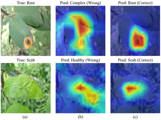
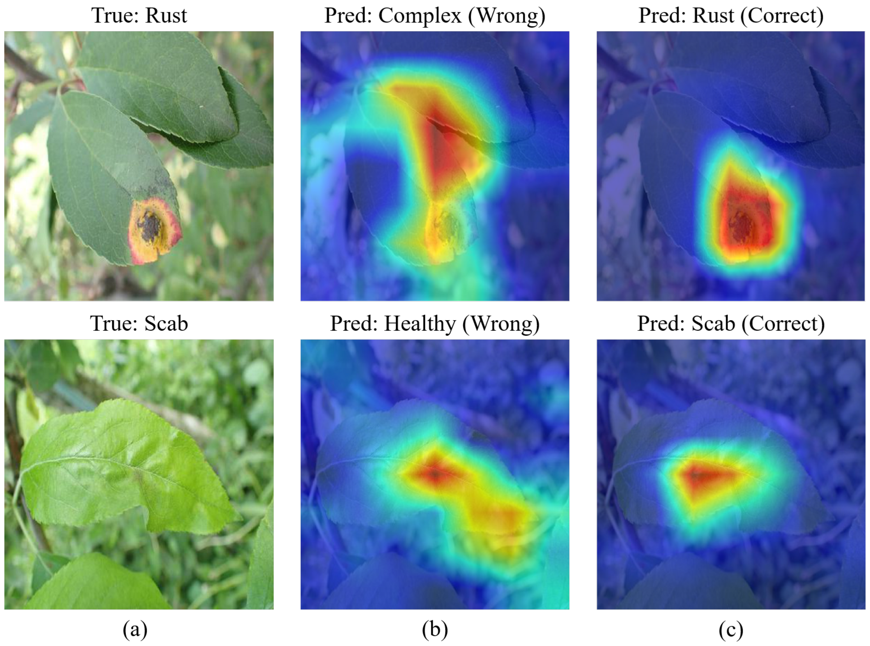
To analyze the reasons behind the model’s performance improvement, we employed Grad-CAM++ [36] to visualize the contributions of different image regions to classification outcomes. Figure 11 highlights two cases. In the first case (true label: rust), the baseline SN-DA model incorrectly predicts the sample as “complex,” with its heatmap focusing mainly on leaf edges and background areas. Conversely, our model accurately predicts “rust,” concentrating its attention precisely on the rust lesion at the leaf’s leading edge. In the second case (true label: scab), subtle early symptoms resemble healthy leaves, leading the baseline model to misclassify it as healthy, with attention focused on healthy leaf regions. Our model, however, successfully detects these subtle pathological features, correctly classifying the leaf as scab, with the heatmap accurately pinpointing the lesion location. These results demonstrate that our method possesses superior symptom localization capabilities, effectively suppressing background noise and enhancing recognition accuracy.

Figure 11. Visual analysis of Grad-CAM++ visualizations between the baseline model and ours: (a) original images, (b) baseline model, and (c) proposed model.

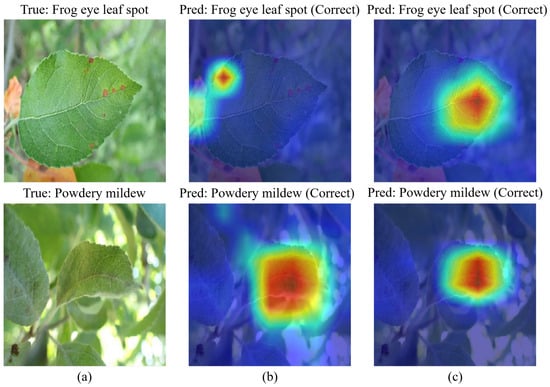
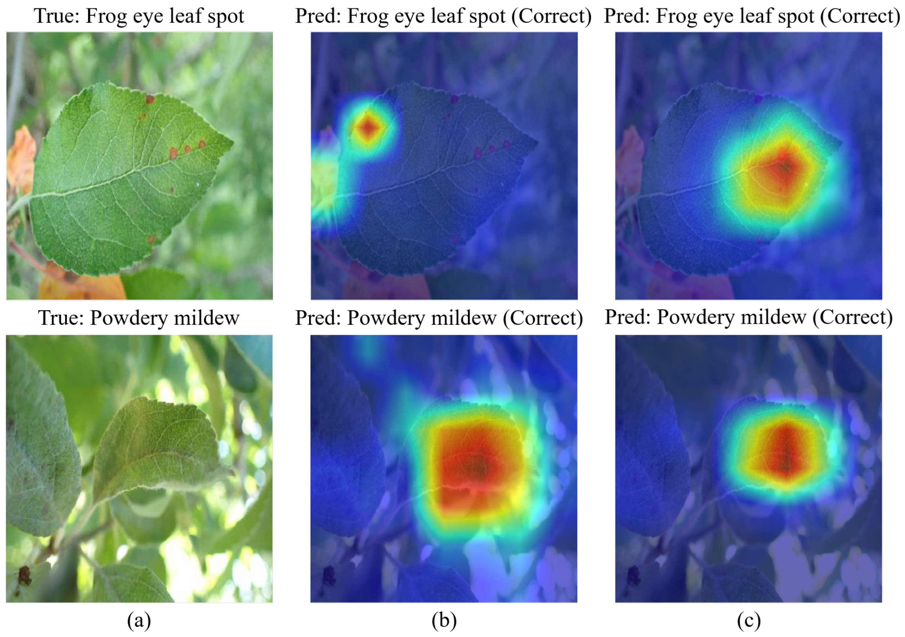
Figure 12 presents the visualization results when both models predict correctly. The findings reveal that even when different methods yield identical predictions, their regions of focus exhibit significant differences. In the frog eye leaf spot case, our model demonstrates more accurate and focused attention compared to the baseline model. The heatmap clearly and precisely marks the exact location of frog eye leaf spot symptoms, eliminating interference from irrelevant background areas. In contrast, the heatmap generated by the baseline model for the powdery mildew case shows a large, broad, and non-specific area, failing to pinpoint the location of symptom occurrence. In contrast, the heatmaps generated by our method narrowed and concentrated on the core areas of powdery mildew lesions on the leaves. These visualizations validate that our approach can learn more precise and relevant expressions of lesion features. Even on correctly classified samples, the feature saliency remains more stable and reliable.

Figure 12. Visual analysis of Grad-CAM++ visualizations, demonstrating the improved attention focus of our proposed model: (a) original images, (b) baseline model’s attention, and (c) proposed model’s attention.

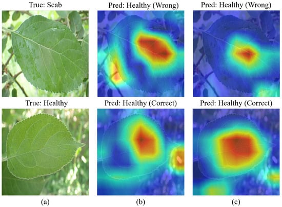
In the confusion matrix analysis, significant cross-classification errors exist between the scab and healthy categories. Figure 13 illustrates the visual similarity between images classified as scab and healthy. It is observed that scab exhibits no obvious symptoms on leaf surfaces during the early stages of infection, or only slight color changes at the leaf tips. Most of the affected area remains visually indistinguishable from healthy leaves, leading the model to misclassify these samples. This visual indistinguishability is likely the primary cause of current classification errors.

Figure 13. Visual analysis of ‘Scab’ and ‘Healthy’ misclassifications: (a) original images, (b) baseline model, and (c) proposed model.

5. Conclusions

Amid the rise of smart agriculture, deep learning has become a dominant technology for automated, real-time plant disease identification. However, high-performance models typically demand substantial computational resources, limiting their deployment on resource-constrained edge devices. To address this, this paper proposes a lightweight, modified architecture based on ShuffleNetV2 0.5×. It incorporates a multi-scale deep convolutional module to capture symptoms across scales, combines a coordinate attention mechanism to focus on key visual features, and employs knowledge distillation to transfer knowledge from a large teacher model. This design significantly enhances the student model’s recognition performance while maintaining computational efficiency.

Although our approach effectively classifies most disease categories, several limitations remain. First, the confusion matrix analysis indicates that the model’s recognition performance can improve when handling categories with mixed symptoms, such as the complex category. Second, validation was primarily performed on a single public dataset; future evaluations should include more diverse datasets encompassing varying geographic regions, imaging conditions, and apple varieties to thoroughly assess generalization capabilities. Based on these insights, future research directions include: (1) developing specialized optimization strategies for the complex category, such as multi-label classification, attention mechanisms tailored to overlapping features, or multi-task learning architectures; (2) deploying the model on actual edge computing devices for field testing and exploring advanced model compression to meet strict hardware constraints; and (3) integrating object detection or segmentation techniques to enable more precise lesion localization and severity assessment.

References

- Thapa, R.; Zhang, K.; Snavely, N.; Belongie, S.; Khan, A. The Plant Pathology Challenge 2020 Data Set to Classify Foliar Disease of Apples. Appl. Plant Sci. 2020, 8, e11390. [Google Scholar] [CrossRef] [Scilit]
- Jafar, A.; Bibi, N.; Naqvi, R.A.; Sadeghi-Niaraki, A.; Jeong, D. Revolutionizing Agriculture with Artificial Intelligence: Plant Disease Detection Methods, Applications, and Their Limitations. Front. Plant Sci. 2024, 15, 1356260. [Google Scholar] [CrossRef] [Scilit]
- Prasad, S.; Peddoju, S.K.; Ghosh, D. Multi-Resolution Mobile Vision System for Plant Leaf Disease Diagnosis. Signal Image Video Process. 2016, 10, 379–388. [Google Scholar] [CrossRef] [Scilit]
- Chuanlei, Z.; Shanwen, Z.; Jucheng, Y.; Yancui, S.; Jia, C. Apple Leaf Disease Identification Using Genetic Algorithm and Correlation Based Feature Selection Method. Int. J. Agric. Biol. Eng. 2017, 10, 74–83. [Google Scholar]
- Sabrol, H.; Satish, K. Tomato Plant Disease Classification in Digital Images Using Classification Tree. In Proceedings of the 2016 International Conference on Communication and Signal Processing, Melmaruvathur, India, 6–8 April 2016; pp. 1242–1246. [Google Scholar]
- Al Bashish, D.; Braik, M.; Bani-Ahmad, S. A Framework for Detection and Classification of Plant Leaf and Stem Diseases. In Proceedings of the 2010 International Conference on Signal and Image Processing, Chennai, India, 15–17 December 2010; pp. 113–118. [Google Scholar]
- Anand, R.; Veni, S.; Aravinth, J. An Application of Image Processing Techniques for Detection of Diseases on Brinjal Leaves Using K-Means Clustering Method. In Proceedings of the 2016 International Conference on Recent Trends in Information Technology, Chennai, India, 8–9 April 2016; pp. 1–6. [Google Scholar]
- Kumar, A.; Nelson, L.; Gomathi, S. Transfer Learning of VGG19 for the Classification of Apple Leaf Diseases. In Proceedings of the 2024 2nd International Conference on Intelligent Data Communication Technologies and Internet of Things, Bengaluru, India, 4–6 January 2024; pp. 1643–1648. [Google Scholar]
- Sulistyowati, T.; Purwanto, P.; Zami, F.A.; Pramunendar, R.A. VGG16 Deep Learning Architecture Using Imbalance Data Methods for the Detection of Apple Leaf Diseases. Monet. J. Keuang. Dan Perbank. 2023, 11, 41–53. [Google Scholar] [CrossRef] [Scilit]
- Chen, Y.; Pan, J.; Wu, Q. Apple Leaf Disease Identification via Improved CycleGAN and Convolutional Neural Network. Soft Comput. 2023, 27, 9773–9786. [Google Scholar] [CrossRef] [Scilit]
- Bi, C.; Wang, J.; Duan, Y.; Fu, B.; Kang, J.R.; Shi, Y. MobileNet Based Apple Leaf Diseases Identification. Mob. Netw. Appl. 2022, 27, 172–180. [Google Scholar] [CrossRef] [Scilit]
- Chao, X.; Sun, G.; Zhao, H.; Li, M.; He, D. Identification of Apple Tree Leaf Diseases Based on Deep Learning Models. Symmetry 2020, 12, 1065. [Google Scholar] [CrossRef] [Scilit]
- Yu, H.; Cheng, X.; Chen, C.; Heidari, A.A.; Liu, J.; Cai, Z.; Chen, H. Apple Leaf Disease Recognition Method with Improved Residual Network. Multimed. Tools Appl. 2022, 81, 7759–7782. [Google Scholar] [CrossRef] [Scilit]
- Fu, B.; Li, S.; Sun, Y.; Mu, Y.; Hu, T.; Gong, H. Lightweight-Convolutional Neural Network for Apple Leaf Disease Identification. Front. Plant Sci. 2022, 13, 831219. [Google Scholar] [CrossRef] [Scilit] [PubMed]
- Yu, H.J.; Son, C.H. Leaf Spot Attention Network for Apple Leaf Disease Identification. In Proceedings of the IEEE/CVF Conference on Computer Vision and Pattern Recognition Workshops, Seattle, WA, USA, 14–19 June 2020; pp. 52–53. [Google Scholar]
- Luo, Y.; Sun, J.; Shen, J.; Wu, X.; Wang, L.; Zhu, W. Apple Leaf Disease Recognition and Sub-Class Categorization Based on Improved Multi-Scale Feature Fusion Network. IEEE Access 2021, 9, 95517–95527. [Google Scholar] [CrossRef] [Scilit]
- Si, H.; Li, M.; Li, W.; Zhang, G.; Wang, M.; Li, F.; Li, Y. A Dual-Branch Model Integrating CNN and Swin Transformer for Efficient Apple Leaf Disease Classification. Agriculture 2024, 14, 142. [Google Scholar] [CrossRef] [Scilit]
- Ait Nasser, A.; Akhloufi, M.A. A Hybrid Deep Learning Architecture for Apple Foliar Disease Detection. Computers 2024, 13, 116. [Google Scholar] [CrossRef] [Scilit]
- Wang, S.; Miao, Z.; Cao, Y. A Lightweight Leaf Disease Recognition Model for MobileNetV2 Based on Transfer Learning and Knowledge Distillation. In Proceedings of the 2024 6th International Conference on Communications, Information System and Computer Engineering, Guangzhou, China, 10–12 May 2024; pp. 459–462. [Google Scholar]
- Ma, N.; Zhang, X.; Zheng, H.T.; Sun, J. ShuffleNet V2: Practical Guidelines for Efficient CNN Architecture Design. In Proceedings of the 15th European Conference on Computer Vision; Lecture Notes in Computer Science; Springer: Berlin/Heidelberg, Germany, 2018; Volume 11218, pp. 122–138. [Google Scholar]
- Hou, Q.; Zhou, D.; Feng, J. Coordinate Attention for Efficient Mobile Network Design. In Proceedings of the 2021 IEEE/CVF Conference on Computer Vision and Pattern Recognition, Nashville, TN, USA, 19–25 June 2021; pp. 13708–13717. [Google Scholar]
- Hinton, G.; Vinyals, O.; Dean, J. Distilling the Knowledge in a Neural Network. arXiv 2015, arXiv:1503.02531. [Google Scholar] [CrossRef] [Scilit]
- Wang, Y.; Wang, Y.; Zhao, J. MGA-YOLO: A Lightweight One-Stage Network for Apple Leaf Disease Detection. Front. Plant Sci. 2022, 13, 927424. [Google Scholar]
- Chang, D.; Tong, Y.; Du, R.; Hospedales, T.; Song, Y.Z.; Ma, Z. An Erudite Fine-Grained Visual Classification Model. In Proceedings of the 2023 IEEE/CVF Conference on Computer Vision and Pattern Recognition, Vancouver, BC, Canada, 17–24 June 2023; pp. 7268–7277. [Google Scholar]
- Plant Pathology 2021-FGVC8. Available online: https://www.kaggle.com/competitions/plant-pathology-2021-fgvc8 (accessed on 2 December 2025).
- Yang, Q.; Duan, S.; Wang, L. Efficient Identification of Apple Leaf Diseases in the Wild Using Convolutional Neural Networks. Agronomy 2022, 12, 2784. [Google Scholar] [CrossRef] [Scilit]
- Cubuk, E.D.; Zoph, B.; Shlens, J.; Le, Q.V. Randaugment: Practical Automated Data Augmentation with a Reduced Search Space. In Proceedings of the 2020 IEEE/CVF Conference on Computer Vision and Pattern Recognition Workshops, Seattle, WA, USA, 14–19 June 2020; pp. 3008–3017. [Google Scholar]
- Woo, S.; Park, J.; Lee, J.Y.; Kweon, I.S. CBAM: Convolutional Block Attention Module. In Proceedings of the 15th European Conference on Computer Vision; Lecture Notes in Computer Science; Springer: Berlin/Heidelberg, Germany, 2018; Volume 11211, pp. 3–19. [Google Scholar]
- Wang, Q.; Wu, B.; Zhu, P.; Li, P.; Zuo, W.; Hu, Q. ECA-Net: Efficient Channel Attention for Deep Convolutional Neural Networks. In Proceedings of the 2020 IEEE/CVF Conference on Computer Vision and Pattern Recognition, Seattle, WA, USA, 13–19 June 2020; pp. 11531–11539. [Google Scholar]
- Zhang, Q.L.; Yang, Y.B. SA-Net: Shuffle Attention for Deep Convolutional Neural Networks. In Proceedings of the 2021 IEEE International Conference on Acoustics, Speech and Signal Processing, Toronto, ON, Canada, 6–11 June 2021; pp. 2235–2239. [Google Scholar]
- Yu, Y.; Zhang, Y.; Cheng, Z.; Song, Z.; Tang, C. MCA: Multidimensional Collaborative Attention in Deep Convolutional Neural Networks for Image Recognition. Eng. Appl. Artif. Intell. 2023, 126, 107079. [Google Scholar] [CrossRef] [Scilit]
- Iandola, F.N.; Han, S.; Moskewicz, M.W.; Ashraf, K.; Dally, W.J.; Keutzer, K. SqueezeNet: AlexNet-Level Accuracy with 50x Fewer Parameters and <0.5MB Model Size. arXiv 2016, arXiv:1602.07360. [Google Scholar]
- Qin, D.; Leichner, C.; Delakis, M.; Fornoni, M.; Luo, S.; Yang, F.; Howard, A. MobileNetV4: Universal Models for the Mobile Ecosystem. In Proceedings of the 18th European Conference on Computer Vision; Lecture Notes in Computer Science; Springer: Berlin/Heidelberg, Germany, 2025; Volume 15098, pp. 78–96. [Google Scholar]
- Tang, Y.; Han, K.; Guo, J.; Xu, C.; Xu, C.; Wang, Y. GhostNetV2: Enhance Cheap Operation with Long-Range Attention. Adv. Neural Inf. Process. Syst. 2022, 35, 9969–9981. [Google Scholar]
- Tan, M.; Le, Q. EfficientNetV2: Smaller Models and Faster Training. In Proceedings of the 38th International Conference on Machine Learning; PMLR 139; ML Research Press: Cambridge MA, USA, 2021; pp. 10096–10106. [Google Scholar]
- Chattopadhay, A.; Sarkar, A.; Howlader, P.; Balasubramanian, V.N. Grad-CAM++: Generalized Gradient-Based Visual Explanations for Deep Convolutional Networks. In Proceedings of the 2018 IEEE Winter Conference on Applications of Computer Vision, Lake Tahoe, NV, USA, 12–15 March 2018; pp. 839–847. [Google Scholar]
Disclaimer/Publisher’s Note: The statements, opinions and data contained in all publications are solely those of the individual author(s) and contributor(s) and not of MDPI and/or the editor(s). MDPI and/or the editor(s) disclaim responsibility for any injury to people or property resulting from any ideas, methods, instructions or products referred to in the content. |
© 2026 by the authors. Licensee MDPI, Basel, Switzerland. This article is an open access article distributed under the terms and conditions of the Creative Commons Attribution (CC BY) license.