


Abstract
Differential Evolution (DE), Teaching–Learning-Based Optimization (TLBO), Grey Wolf Optimizer (GWO), and the Ali Baba and the Forty Thieves Algorithm (AFTA) are compared for switching angle calculation in an ideal seven-level single-phase cascaded H-bridge inverter. Each method uses 30 paired seeds, 1000 candidates, and 201,000 objective-function evaluations. The common objective combines voltage THD through the 49th harmonic with absolute fundamental voltage error relative to 250 V peak. DE and AFTA attain THD49 = 11.6691079% and meet the empirical target in all 30 runs; TLBO succeeds in 2 runs and GWO in none. DE requires a median of 29,361 evaluations to reach the target, compared with 53,822.5 for AFTA. AFTA has the lowest mean full-budget runtime, 1.2354 s, versus 2.0742 s for DE. Paired tests with multiplicity correction distinguish DE/AFTA from TLBO/GWO in final objective value, but do not distinguish DE from AFTA at the declared numerical resolution. The maximum separation between the best THD values is only 0.0004657 percentage points. The results separate numerical precision, search effort, and runtime within one analytical operating condition; they do not establish global optimality or a practically significant electrical advantage.
Keywords:
multilevel inverter; cascaded H-bridges; switching angles; THD; optimization; DE; TLBO; GWO; AFTA 1. Introduction
Multilevel inverters allow for the synthesis of a stepped voltage from various direct current sources and, through an appropriate selection of switching instants, allow the output waveform to approximate a sinusoidal signal. Among the most studied configurations is the cascaded H-bridge (CHB) inverter, whose modular structure allows for obtaining multiple voltage levels by connecting cells in series. A systematic review of metaheuristic methods applied to harmonic distortion reduction reported that seven-level case studies, the CHB topology, and RL loads appear frequently in the literature, particularly when evolutionary algorithms are employed [1].
In a symmetric seven-level single-phase CHB, three switching angles in the first quarter cycle determine the fundamental component and the odd harmonic components of the voltage. Therefore, the selection of the angles can be formulated as a nonlinear optimization problem subject to order and interval constraints. The minimization of harmonic distortion should not be considered in isolation: a set of angles can reduce the THD while simultaneously modifying the amplitude of the fundamental. In a previous study with Differential Evolution (DE), a sweep of the modulation index produced different sets of angles and different THD values, highlighting the need to declare the voltage reference and evaluation conditions before comparing algorithms [2].
Population-based metaheuristics constitute an alternative for exploring this search space without relying on a single initial condition. DE uses mutation, crossover, and selection operations; Teaching–Learning-Based Optimization (TLBO) organizes the search into a teacher phase and a student phase. A review of 62 papers published between 2013 and 2021 showed the application of TLBO in different areas of electronic engineering, including power electronics and multilevel inverters, and highlighted its low need for specific initialization parameters [3]. Moreover, TLBO has already been directly applied to the minimization of THD in a seven-level CHB and compared with GA, DE, and PSO through a modulation index sweep [4].
The present work compares DE, TLBO, Grey Wolf Optimizer (GWO), and the Ali Baba and the Forty Thieves Algorithm (AFTA). Due to the fact that the internal structure of these algorithms is not equivalent, the number of iterations does not necessarily represent the same search cost. In particular, TLBO generates proposals both in the teacher phase and in the student phase. For this reason, the comparison is carried out using a common budget of objective-function evaluations and is repeated with multiple seeds. In addition to the final THD, the regulation of the fundamental component, the dispersion between executions, the convergence trajectory, and the computation time are analyzed.
The study asks whether methods that produce nearly identical best voltage spectra also require similar search effort and computational time. Earlier DE and TLBO studies already establish their relevance to seven-level CHB optimization [2,4]; the present contribution is therefore a controlled numerical comparison, not a new topology or optimizer. Its distinguishing measurements are paired run-level inference, the distribution of evaluations and elapsed time to an empirical target, and separate timing passes under a common evaluation budget. Incorporating GWO and AFTA permits these indicators to be compared across four search mechanisms. The experiment remains restricted to one 250 V peak reference and a fixed parameter configuration; it does not establish a universal performance ranking.
2. Materials and Methods
2.1. Seven-Level CHB Inverter Model
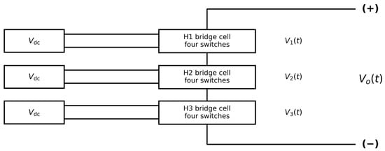
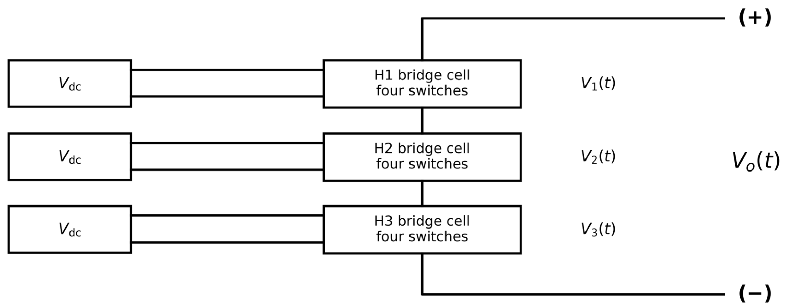
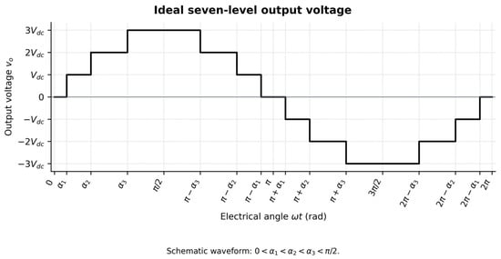
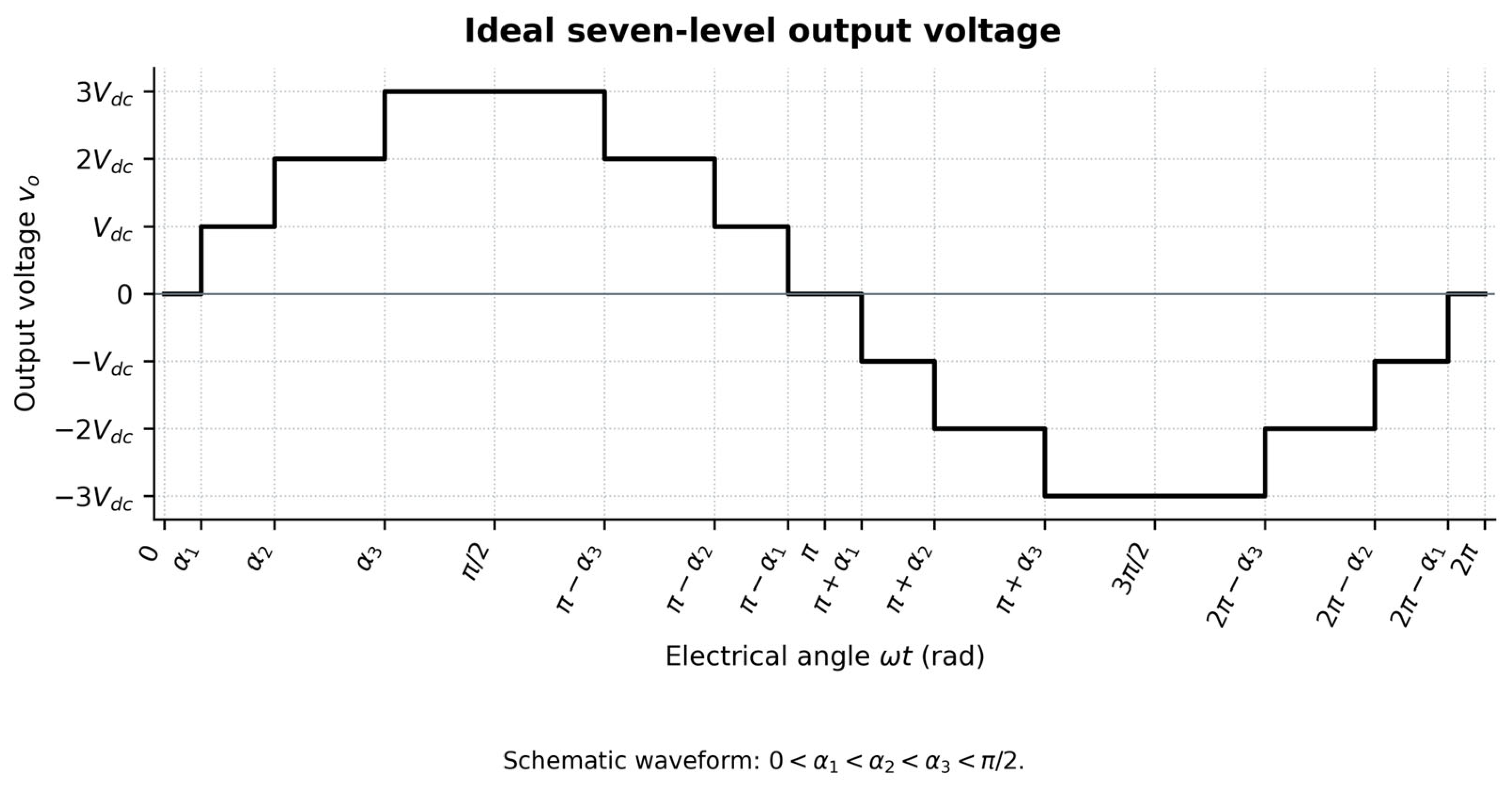
The single-phase inverter consists of three H-bridge cells connected in series. Each cell has a DC source Vdc and four switches, and supplies +Vdc, 0 or −Vdc. The combined output has seven levels: −3Vdc, −2Vdc, −Vdc, 0, Vdc, 2Vdc and 3Vdc. With m equal-source cells, the number of levels is 2m + 1; therefore, m = 3 produces seven levels. Figure 1 shows the conceptual topology [1,2], and Figure 2 illustrates the ideal stepped voltage.
Figure 1.
Conceptual configuration of the seven-level single-phase CHB.
Figure 2.
Ideal seven-level waveform and switching angles.
The waveform considered has half-wave and quarter-wave symmetry: its second half is the negative of the first, and the segments of each semicycle are symmetric. Thus, the DC component and the even harmonics cancel out, and the pattern is defined with three angles in the first quadrant. The strict order in Equation (1) maintains the sequence of the steps.
The amplitude of the odd harmonic n is obtained using the Fourier series:
Even harmonics cancel under the assumed symmetry. Each source is fixed at Vdc = 83.33 V and the only decision variables are α1, α2 and α3. Consequently, an algorithm cannot reduce the objective by changing the source voltages. The equations use radians, whereas the MATLAB implementation stores angles in degrees and evaluates trigonometric terms with cosd.
2.2. Formulation of THD Minimization
Harmonic quality is evaluated using the THD of voltage truncated to the order H = 49. Equation (3) includes the odd components from n = 3 to n = 49 and uses the magnitude of the fundamental component as a reference. The same set of orders is used for all algorithms. The ratio has the same value whether peak amplitudes or RMS values are used, provided that the same conventions is used in the numerator and denominator.
To prevent a reduction in THD at the expense of an inadequate fundamental amplitude, the scalar function from Equation (4) is used. The reference is peak, and the weighting is λV = 10 units of the objective function per volt. The formulation constitutes a weighted sum of distortion and absolute voltage error; it is not a Pareto multi-objective optimization. Its interpretation requires keeping the percentage scale of THD and the voltage unit constant.
The voltage error term uses an absolute value. This expression was checked against objetivo_chb in the executed CHB_UNIFICADO_usado.m source and independently against all 120 exported final results.
Angular feasibility is handled separately from J. The shared reparar_angulos_71 routine clips, orders, and separates candidate angles; objetivo_chb checks strict ordering and returns a feasibility flag. Feasible solutions are compared by J, while infeasible candidates are rejected using the common feasibility-first rule. The same model, repair, and comparison routines are used by all four methods.
2.3. Optimization Methods
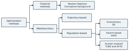
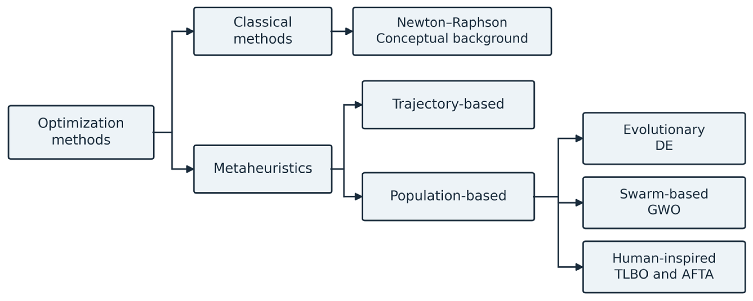
Four population-based metaheuristics are evaluated quantitatively. Figure 3 distinguishes these methods from Newton–Raphson (NR), which is included only as deterministic background. The benchmark assesses feasibility and the common objective value; agreement between methods does not prove global optimality.
Figure 3.
Selected optimization methods and the position of NR, DE, TLBO, GWO and AFTA.
DE is an evolutionary method [5]; GWO is inspired by the hunting behavior of a wolf pack [6]; TLBO and AFTA use analogies to human activities [7,8]. The term population-based metaheuristics there-fore describes this set more accurately than bio-inspired algorithms. All benchmarked methods share the electrical model, objective, and angular repair routine. NR is not included in the 120 runs or in their statistical summaries.
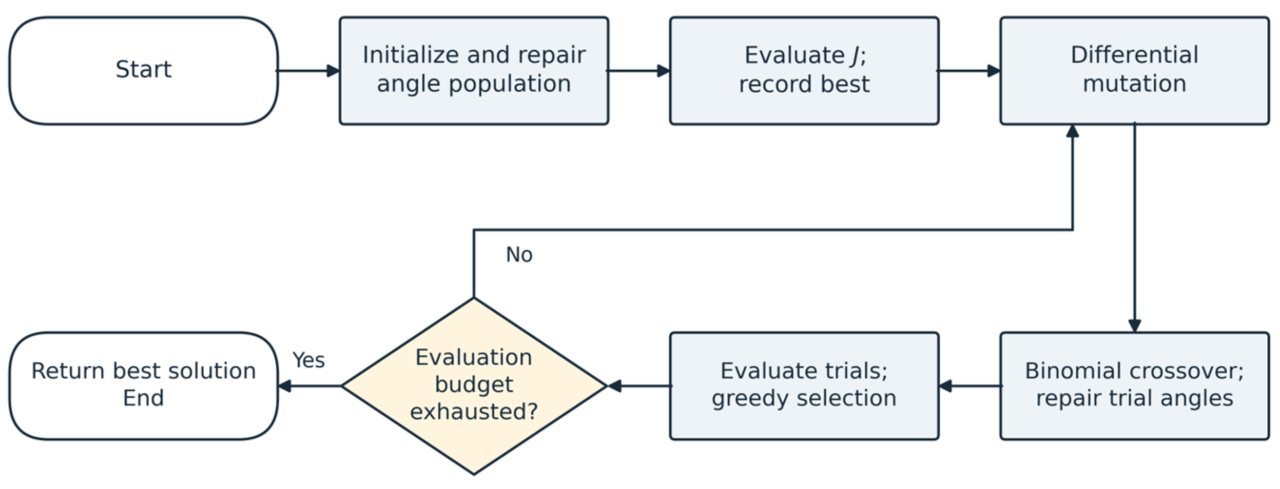
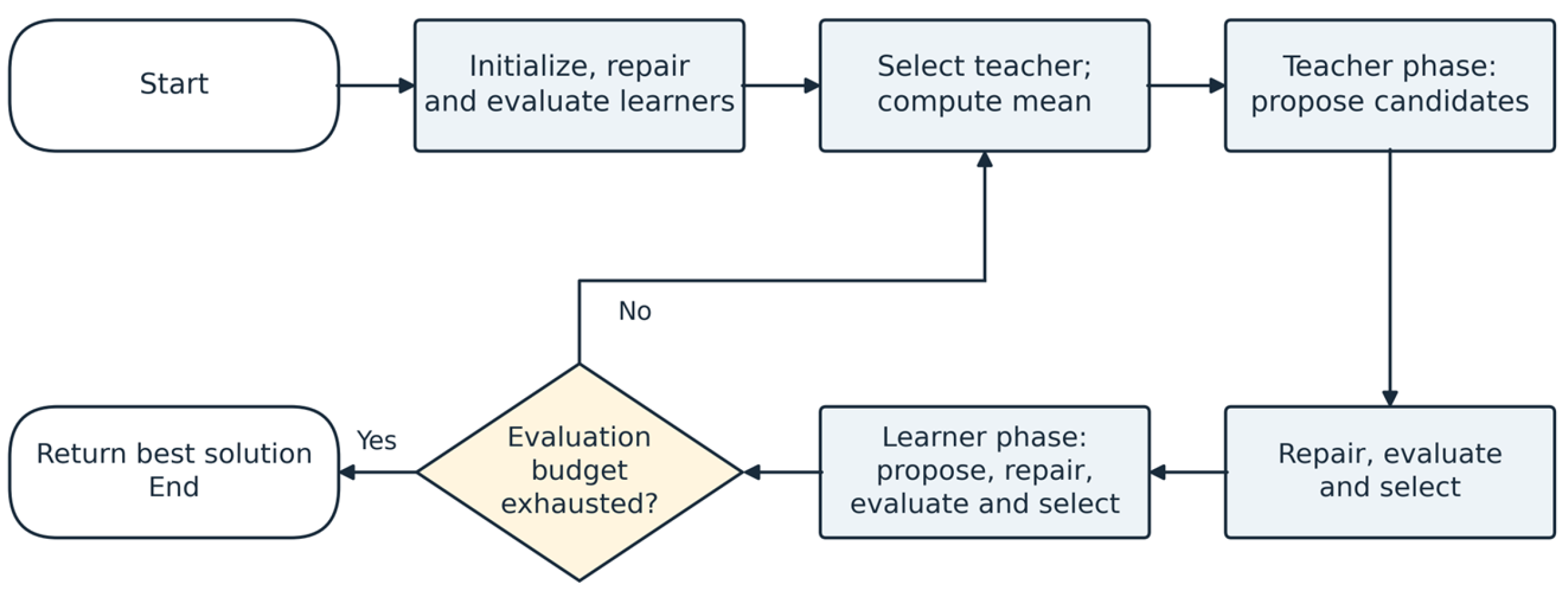
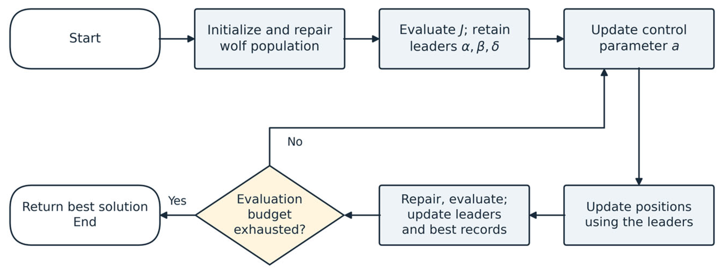
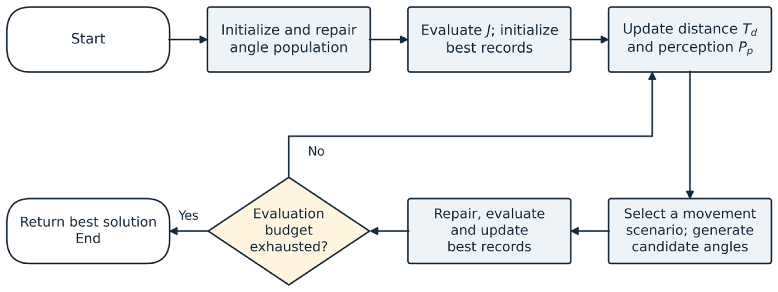
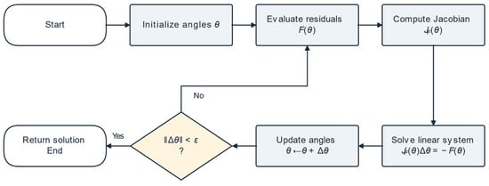
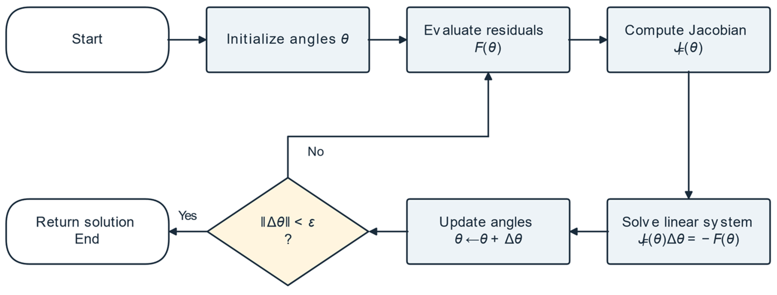
Figure 4 is retained only as conceptual Newton-Raphson background; NR contributes no observations to the statistical analysis. Figure 5, Figure 6, Figure 7 and Figure 8 summarize the implementations used in the benchmark and identify the generation, repair, and evaluation stages charged to the common budget. The executable source in the reproducibility package specifies update order, random number consumption, and acceptance rules. The diagrams support reproducibility and are not presented as novel algorithms.
Figure 4.
Conceptual Newton–Raphson procedure; not executed in the benchmark.
2.3.1. Newton–Raphson
NR iteratively solves a linear system formed from the Jacobian of a nonlinear harmonic equation system and then updates the angle vector. Termination may depend on the residual norm or correction norm. Local convergence does not replace checks of angular limits, ordering, or fundamental voltage magnitude. Figure 4 summarizes this conceptual procedure; previous angle calculation studies provide its application context [9,10,11,12,13,14].
Solving specific harmonic equations does not automatically equate to minimizing the function J of this study. Moreover, J contains a non-differentiable absolute value when V1 = 250 V, so it is not appropriate to simply attribute a direct application of the classical method to it. No implementation or results of NR under a comparable protocol are presented here; its inclusion is conceptual.
The background on angle calculation includes the comparison of NR, PSO, and GA [9], the combined use of neural networks and NR [10], and the evaluation of NR and PSO for harmonic mitigation [11]. Implementations of SHEPWM with NR and dSPACE [12], angle control in CHB inverters using NR [13], and selective harmonic elimination on FPGA [14] have also been described. These works provide context for the deterministic method; their formulations and platforms may not match the THD minimization experiment presented here.
2.3.2. Differential Evolution
The implemented DE/rand/1/bin operator uses three distinct donors different from the target individual [5]. The mutant is repaired before binomial crossover; crossover forces at least one mutant component and is followed by another repair. Accepted candidates update the population in place, so later proposals can use already updated individuals. F = 0.3 and CR = 0.9 are fixed experimental settings, not values established as optimal for this problem. Figure 5 summarizes the sequence.
The use of DE for the calculation of angles in a seven-level CHB has direct precedents in simulation and experimental validation [2].
The evolution of DE is documented in a review of its recent developments [15]. Among the strategies studied are the combination of various search mechanisms [16], the ordering of crossover rates in adaptive DE [17], hierarchical mutation and selection with two populations [18], and the analysis of population size [19]. These precedents allow us to distinguish the DE/rand/1/bin configuration used here from other variants; the present experiment does not evaluate those modifications. The size of 1000 individuals is a common experimental condition and is not interpreted as the optimal size for all methods.
Figure 5.
DE flow applied to the three angles.
2.3.3. Teaching–Learning-Based Optimization
TLBO uses a teacher phase and a learner phase [7]. At the start of the teacher phase, the best solution and population mean are fixed, and a teaching factor TF in {1, 2} is selected for that phase. Each proposal adds to the current student a component-wise random weighting of the difference between the teacher and TF times the population mean. After repair and evaluation, the proposal is accepted only if it improves the feasibility-first comparison. In the learner phase, another student is selected; the movement is directed away from a worse peer or toward a better peer, with independent component-wise random weights. Repair, evaluation, and selection follow each proposal. Each phase consumes Np evaluations and has its own convergence record. The basic method has no control parameters corresponding to DE’s F and CR, but population size and evaluation budget still affect its behavior [3,4]. Figure 6 summarizes both phases.
The extensions of TLBO include stochastic crossover, self-learning, and combined learning [20], hybridization with PSO [21], and adaptations for robot trajectory planning [22]. Variants for production scheduling with additional resources [23] and sequencing problems without waiting [24] have also been studied. These are methodological precedents for the TLBO family, while the article on the seven-level CHB [4] directly supports its application to the electrical problem of this study.
Figure 6.
TLBO flow applied to angle calculation.
2.3.4. Grey Wolf Optimizer
GWO uses alpha, beta, and delta leaders [6]. The executed implementation retains the three best historical leaders across batches. Independent random vectors generate three leader guided proposals using component-wise absolute distances; their average forms each candidate. The new population is repaired and evaluated before leader records are updated. The control parameter a decreases from 2 at batch 1 to 0 at batch 200. Figure 7 therefore represents this specific historical leader implementation, rather than every published GWO variant.
A review summarizes versions and applications of GWO [25]. In converters, stepped modulation for symmetric and asymmetric CHB has been studied [26], as have harmonic elimination with PSO and GWO [27], GWO-NR hybridization [28], and firing angles of a 31-level three-phase inverter [29]. Other works examine metaheuristics for selective har-monic elimination at different numbers of levels [30] and a variant of GWO with Lévy flights [31]. These references place the implementation used within a broader family and do not imply that their results are transferable to the present configuration.
Figure 7.
GWO flow applied to the angular vector.
2.3.5. Ali Baba and the Forty Thieves Algorithm
The original method is Ali Baba and the Forty Thieves (AFT) [8]; AFTA is retained here to match the implementation name. The adaptation stores a personal-best position for each candidate and a global best. For search batch k, r = k/200, with k from 1 to 200; initialization is not included in r. The reported schedules are Td = 2exp(−2r2) and Pp = 0.1ln(2.75r0.1). Movement uses differences involving the current position and personal memories, with random choices between exploratory proposals and movement around the global best. The population is repaired and evaluated before personal and global bests are updated. Figure 8 summarizes the adaptation. These schedules are fixed implementation choices; their optimality for this CHB problem has not been established.
The background of AFT includes an improved version for feature selection [32], maximum power point tracking in shaded photovoltaic systems [33], neural network weight adjustment [34], and parameter estimation of a photovoltaic equivalent circuit [35]. A combination of PSO with binary AFT for feature selection has also been published [36]. These applications justify studying these operators in other domains, but they do not constitute validation of the CHB inverter, nor do they replace the common protocol of this work.
Figure 8.
AFTA flow adapted to the angle vector.
2.4. Comparison Criteria
The literature shows various ways to approach angle calculation, including equation solving, direct distortion minimization, and metaheuristic schemes. The background of DE and TLBO in multilevel inverters shows that the conclusions depend on the formulation, the voltage reference, and the evaluation conditions [1,2,3,4]. Consequently, the present comparison is limited to the implemented versions and avoids attributing the advantages observed in a single configuration to the entire family.
Three groups of indicators are used. Electrical quality is described by THD49, the fundamental component, voltage error, and spectrum; numerical performance, by final J, dispersion, and success rate; and computational cost, by evaluations and by execution time. Two methods can produce practically equivalent voltages and differ in the other indicators. Therefore, a small difference in THD should not be presented as sufficient evidence of general superiority.
Shared conditions improve the traceability of the comparison, but do not eliminate its limitations. The observed distribution corresponds to 30 seeds, a fixed population, and a single voltage reference. Harmonic truncation excludes components higher than order 49. The times belong to the environment used and do not constitute a guarantee of performance on another computer or in a real-time controller.
2.5. Configuration and Evaluation Protocol
The numerical experiment uses the ideal Fourier model in Equations (1)–(4), three equal sources of 83.33 V, and a 250 V peak fundamental reference. A nominal 60 Hz frequency and a 100 Ω, 100 mH load are retained as application context only. Neither frequency nor load enters the voltage objective, and the program does not integrate circuit dynamics or calculate load current. Reconstructed waveforms are plotted against electrical angle. Table 1 summarizes the electrical conditions and common evaluation setup.
Table 1.
Electrical conditions and common setup of the evaluation.
Each candidate contains three angles in degrees. The common repair routine clips them to the open interval defined numerically by 10−8° and 90–10−8°, sorts them, and separates coincident values by 10−8°. If necessary, it shifts the row to restore the upper limit and checks the lower limit again. The objective routine verifies strict ordering. Invalid candidates receive J = 1012 and h = 100; feasible candidates have h = 0. Selection favors feasibility and then the smaller J. Because all invalid candidates share h = 100, h does not measure the magnitude of constraint violation.
For every feasible candidate, Equation (2) yields V1 and odd harmonics n = 3, 5, …, 49. Equation (3) then gives THD49. The scalar selection objective is J(α) = THD49(α) + 10|250 − V1(α)|, with voltage in volts and THD in percent. The absolute-value bars apply to the complete voltage difference. This weighted sum is not a Pareto multi-objective formulation.
The program runs 30 independent runs per algorithm with seeds from 1 to 30 and rng (seed, ‘twister’). Each routine begins with the same instruction for uniformly generating a 1000 × 3 component matrix and the same repair. According to the protocol described here, resetting the same seed thus produces the same initial population for the four methods; the subsequent trajectories differ due to the consumption of random numbers and the operators. The 1000 initial evaluations and the 200,000 search evaluations total 201,000 evaluations per run. This corresponds to 200 batches of DE, GWO, and AFTA, and to 100 complete cycles of TLBO, with two phases of 1000 evaluations per cycle. The population is not interpreted as a sample of the physical states of the inverter, but rather as numerical candidates.
Two passes are executed for each method–seed pair. One records every improvement of the best feasible objective, together with its exact evaluation count, angle vector, THD, fundamental voltage, and elapsed time. The second repeats the same seed without this detailed event logging and supplies the full-budget runtime. Both retain a 201-point batch convergence history, and the program checks the agreement of final angles and the objective between passes. Thus, the study contains 120 stochastic results and 120 timing repetitions, not 240 independent observations. A short warm-up precedes measurement; method order rotates across seeds, and the order of the two passes alternates. Timers include initialization, objective evaluation, repair, search operations, and their respective internal bookkeeping, but exclude file export and plotting. Final consistency checks are outside the optimization budget.
For descriptive summaries, the sample mean and standard deviation are reported; THD is also described by its median and interquartile range, using linear interpolation at position 1 + (N − 1)p for quantile fraction p. The empirical target is J ≤ Jref + 0.001 together with |250 − V1| ≤ 0.1 V, where Jref = 11.6691079213354 is the smallest final J in this dataset. The target is retrospective and is not a proven optimum. For each run, the first recorded improvement satisfying both conditions defines evaluations and instrumented time to target. Nonattainment remains missing rather than being replaced by a successful observation at the budget. Conditional means, medians, and standard deviations are interpreted jointly with attainment rates.
The unified program exports run-level results, batch convergence histories, exact improvement events, statistical comparisons and spectra. For each method, the spectrum is computed directly from the full-precision angles of the row minimizing J; it is not transcribed from rounded manuscript values. Reconstructed THD and V1 are checked against that row within 10−8. The supplied dataset contains 120 final rows, 24,120 batch history rows and 6717 improvement events; independent checks reproduced final J and THD within 1.4 × 10⁻¹² and 6.1 × 10⁻¹⁴, respectively. Appendix A identifies the reproducibility files. The source code, original data, and reproduction instructions are provided in the Supplementary Materials (Reproducibility_CHB_minor_revision.zip).
The runs used MATLAB 24.2.0.2712019 (R2024b), PCWIN64, on an AMD Ryzen 7 7445HS with Radeon 740M Graphics. The operating system reported Microsoft Windows version 10.0.26300.9457; detected physical memory was 15.2676 GiB, and MATLAB reported a maximum computational-thread setting of 6. Optimizers ran serially, without parfor or GPU acceleration. These values describe the supplied run environment and do not imply that all six threads were active in every operation.
Inferential analysis treats seed as a block and method as a treatment within this single operating condition. Friedman’s test [37] is applied separately to final J, THD, absolute voltage error and full-budget runtime, with tie correction and an asymptotic chi-square reference. Kendall’s W = χ2/[30(4 − 1)] summarizes rank separation. J is the primary endpoint; other metrics are secondary. Before ranking, values are quantized at 10−9 for J, THD in percentage points, and voltage error in volts, and at 10−6 s for runtime. This prevents floating-point differences from being interpreted as substantive ranks; exported measurements retain their full precision.
Pairwise comparisons use two-sided signed-rank tests [38], with exact sign-assignment distributions, average ranks for ties, and zero differences excluded. Rank-biserial correlation is (W + − W−)/(W + + W−) for A minus B; a negative value favors A because all metrics are minimized. Since signed-rank inference assumes symmetric paired differences under its null, exact paired sign tests are also reported as a sensitivity analysis. Holm adjustment [39] is applied across all 24 pairwise comparisons (six method pairs by four metrics), separately for each test family; the four Friedman p values form another Holm family. These adjustments do not provide joint error control across all three families. All inference is conditional on this implementation, parameter setting, and operating point.
Population size and algorithm parameters are held fixed to define a common baseline, rather than to optimize each method separately. Np = 1000 is an experimental design choice that fixes the number of initial candidates and the allocation of the evaluation budget; it is not derived from the three-dimensional problem size or from a population-tuning study. Using the same population and paired initialization controls these inputs, but does not make the configuration equally favorable to all four search mechanisms. The results therefore constitute a fixed-configuration benchmark, not a comparison of the best attainable performance of each algorithm. Table 2 summarizes the configuration of each method.
Table 2.
Configuration of the considered methods.
At the fixed budget B = 201,000, initialization consumes Np evaluations, and the remaining search comprises B/Np − 1 population-sized batches: 200 at Np = 1000. TLBO uses two such batches per complete teacher–learner cycle, giving 100 cycles. For illustration only, Np = 500 would allow 401 search batches, including 200 complete TLBO cycles and one additional phase; this is budget arithmetic, not a sensitivity result. A larger initial population can broaden the sampled coverage but leaves fewer population-wide updates for refinement. In DE, this changes the donor pool and the number of population sweeps; in TLBO it changes the teacher/peer interactions; and in GWO and AFTA, it changes how many leader or memory updates occur. Their scheduled coefficients must also be interpreted relative to the available batches. Equal evaluation counts do not imply equal runtime because repair, selection, and internal bookkeeping differ. Consequently, target attainment rates, convergence curves, and runtime rankings may change with population size; their direction and magnitude cannot be inferred from the present runs.
3. Results
3.1. Final Quality and Computational Behavior
A total of 120 executions were recorded, 30 for each metaheuristic. The budget per execution was 201,000 evaluations, including the initial population. The final reported solutions respect the angular domain. Table 3 summarizes the angles of the best run according to J and the THD, time, and success statistics. NR is excluded from this table because it was not executed under an equivalent multiple-start protocol.
Table 3.
Results of 30 runs per metaheuristic.
DE and AFTA attained J = THD49 = 11.6691079213 at the displayed precision, with V1 = 250 V and angles approximately [10.157139°, 31.056272°, 58.982498°]. TLBO and GWO reached minimum J values of 11.6698774657 and 11.6701368957, respectively. Their mean THD values exceeded the best observed reference by about 0.00197 and 0.00278 percentage points. Because J also contains voltage error, it must not be interpreted as THD alone.
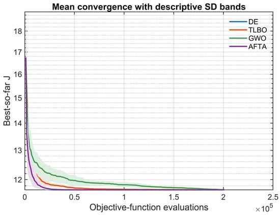
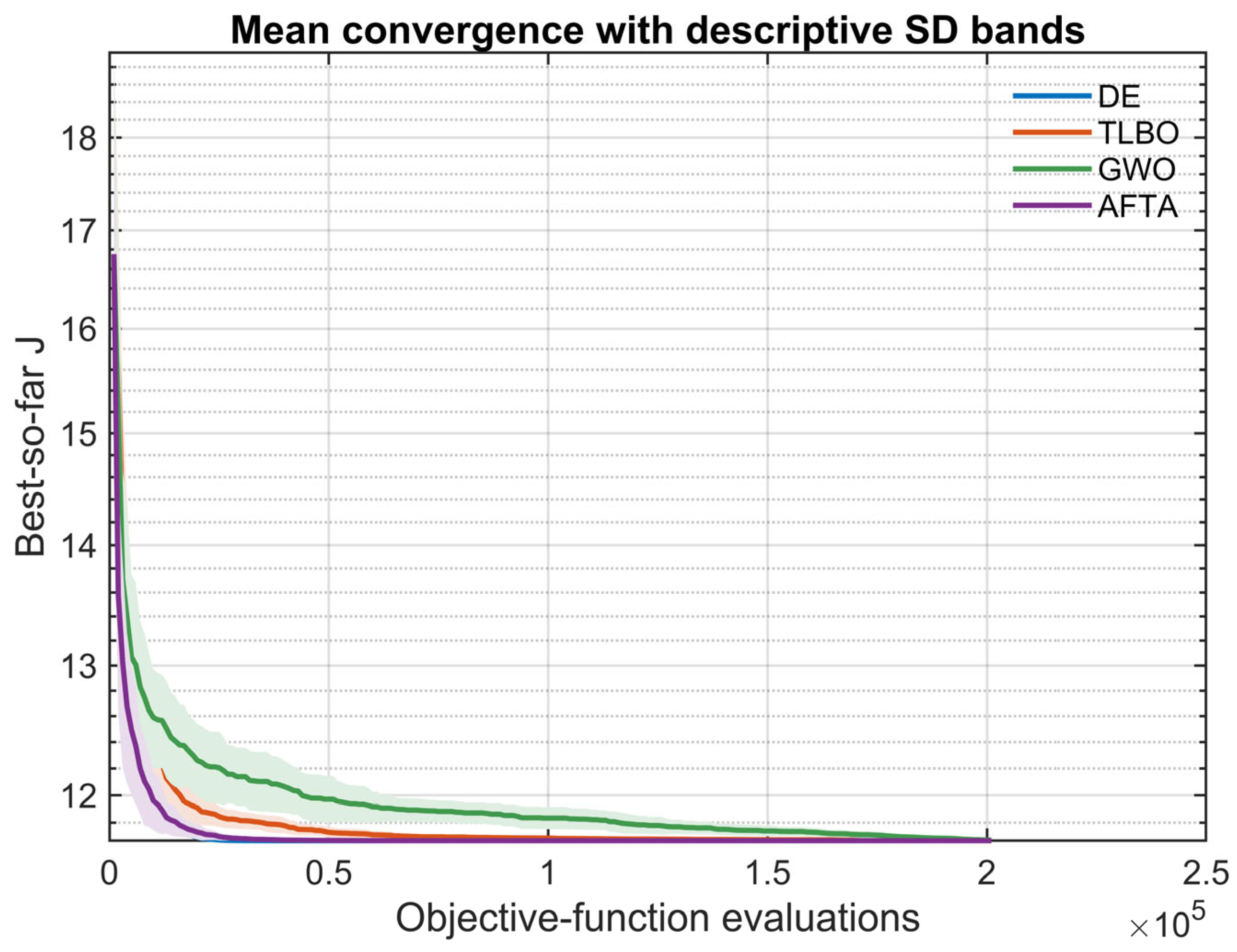
Figure 9 presents mean best-so-far J and one sample standard deviation at common evaluation counts. It describes aggregate convergence, not the distribution of individual first-passage effort. That distribution is analyzed separately in Section 3.4 from exact improvement events, so a crossing of the mean curve is not reported as a typical run’s convergence count.
Figure 9.
Mean best-so-far J versus objective-function evaluations; shaded bands show one sample standard deviation, not confidence intervals.
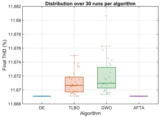
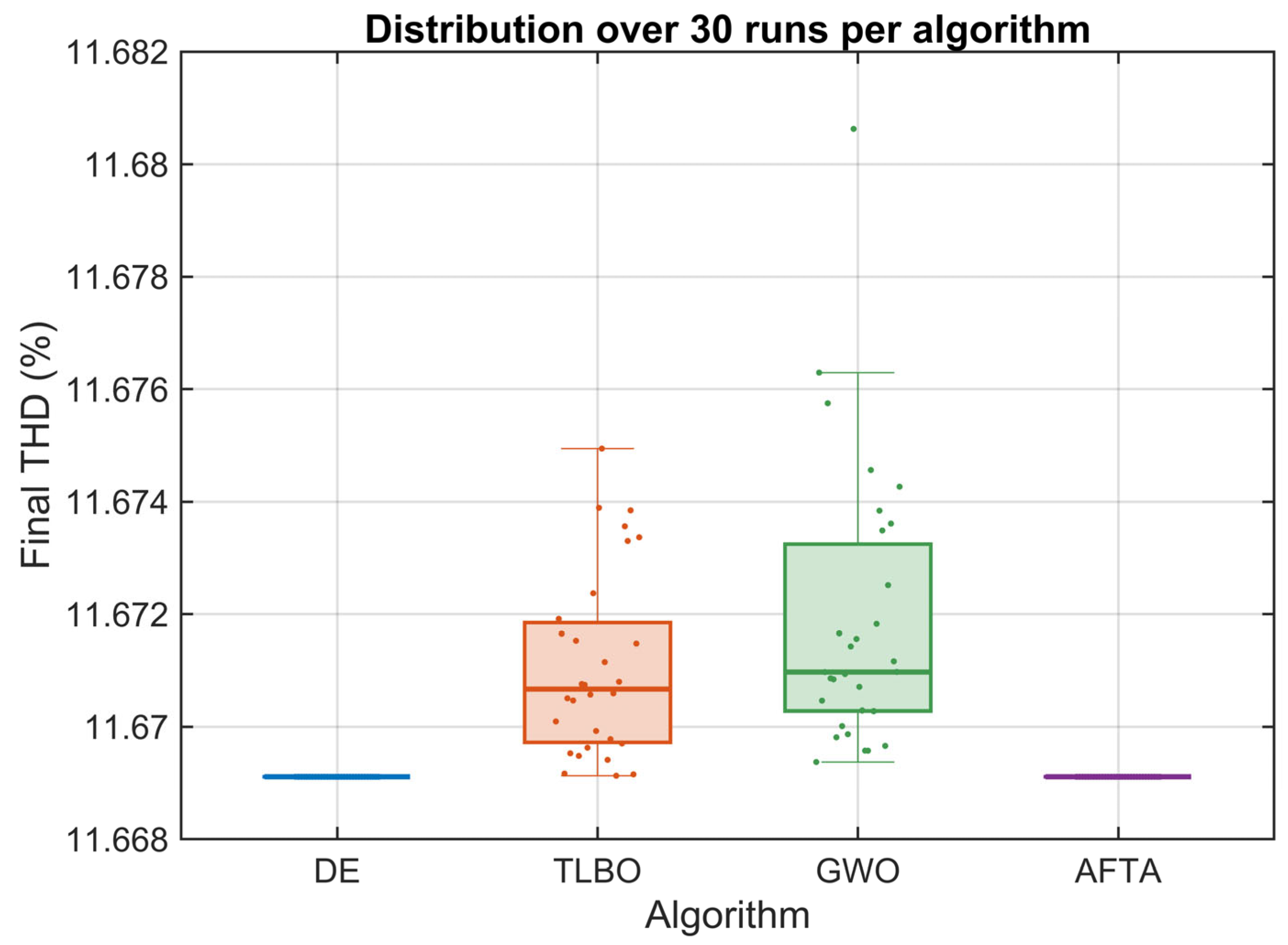
Figure 10 shows the dispersion of THD49. DE and AFTA match the recorded precision. TLBO presents an interquartile range of 0.002128 percentage points and GWO of 0.002965 percentage points. The maximum value for GWO is 11.680628%. The enlargement of the vertical axis allows the variability to be observed, but it should be read together with the absolute magnitude of the differences.
Figure 10.
Final THD49 across 30 runs per method; boxes show quartiles and overlaid points show individual runs.
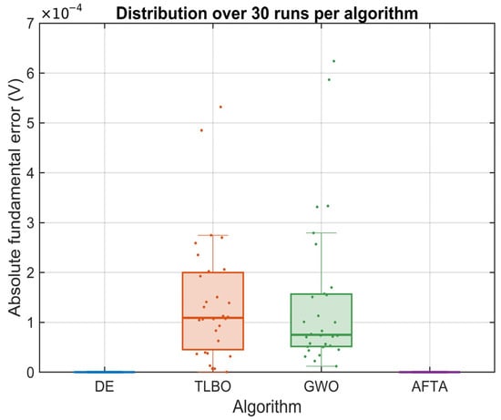
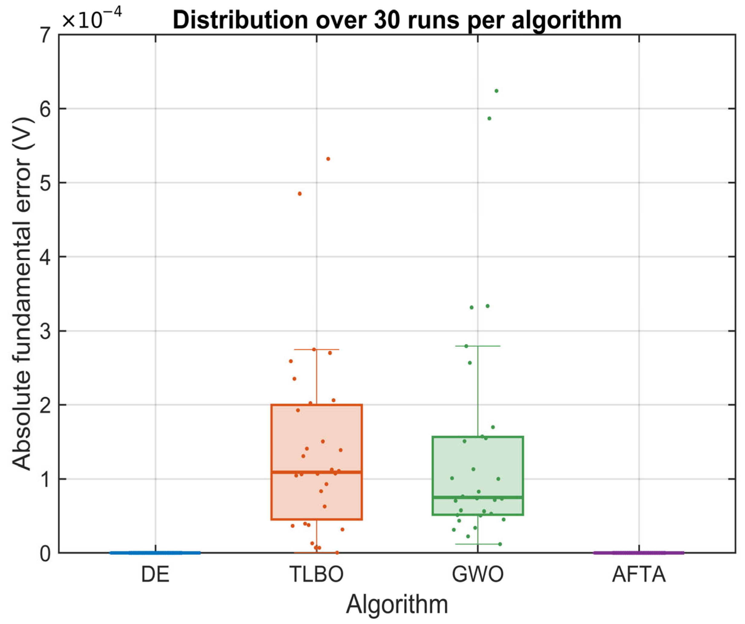
Figure 11 presents the absolute error of the fundamental. In DE and AFTA, it is zero at the stored precision. TLBO and GWO show mean errors of 0.143 mV and 0.142 mV, and maximum values of 0.532 mV and 0.624 mV, respectively. All reported values are below the 0.1 V tolerance established in the protocol.
Figure 11.
Absolute fundamental voltage error |250 − V1| across 30 runs per method.
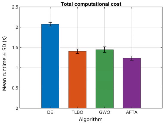
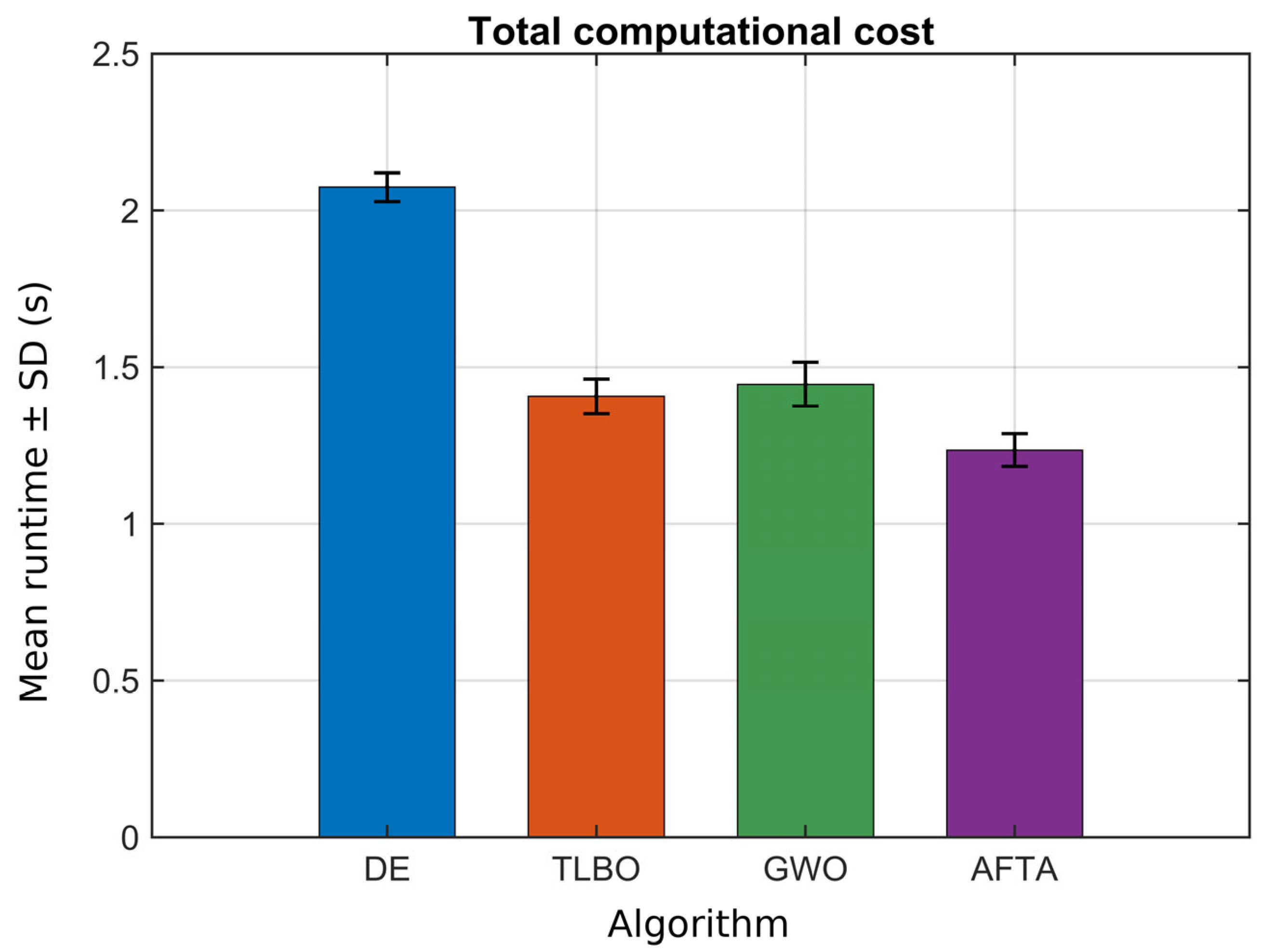
The mean full-budget runtimes without detailed improvement logging were 2.0742 ± 0.0461 s for DE, 1.4068 ± 0.0551 s for TLBO, 1.4451 ± 0.0704 s for GWO, and 1.2354 ± 0.0526 s for AFTA (mean ± sample SD). AFTA’s mean was 40.44% below DE’s in this environment. Dividing total runtime by 201,000 gives 10.3194, 6.9990, 7.1896, and 6.1463 μs per evaluation, respectively. These are amortized total costs, including algorithm and repair operations, not isolated objective-evaluation costs. Figure 12 summarizes the measured times.
Figure 12.
Full-budget runtime without detailed improvement logging; bars and error bars show mean and sample standard deviation over 30 timing passes.
3.2. Fourier Spectra of the Best Solutions
For each algorithm, the run with the lowest J value was selected, and its harmonic content was evaluated using Equation (2). This equation comes from the Fourier series of the stepped voltage with quarter-wave symmetry. For the three cells of the CHB, it can be explicitly written as:
Here Vn is the signed peak Fourier coefficient of odd harmonic order n, Vdc = 83.33 V is the source voltage of each cell, and α1, α2 and α3 are switching angles. The factor 4/(nπ) and the sum of cosines follow from the symmetric stepped waveform. The cosine terms can reinforce or cancel one another. MATLAB evaluations use cosd when angle values are stored in degrees.
When n = 1, Equation (5) yields V1, the fundamental component regulated to 250 V peak. For n = 3, 5, …, 49, it yields the non-fundamental odd components. The sign of Vn indicates the phase or polarity relative to the reference; the spectra therefore display |Vn|. Even orders and the DC component vanish because of the assumed half-wave and quarter-wave symmetries, not because of a particular optimizer.
To compare the four methods without depending on the absolute scale, each harmonic was normalized with respect to the fundamental:
Thus, the bar for n = 1 always equals 100%, while a 6% bar indicates that the peak amplitude of that harmonic is equivalent to 6% of V1. With this normalization, the THD considered in the study (truncated to order 49) is directly reconstructed from the non-fundamental odd bars:
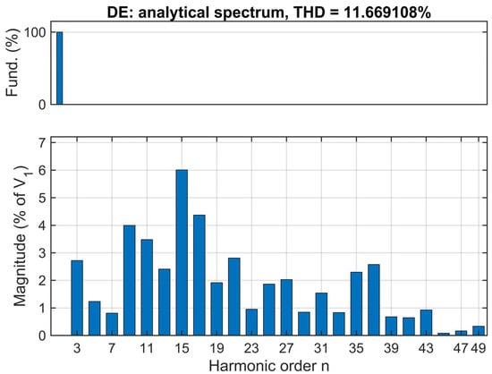
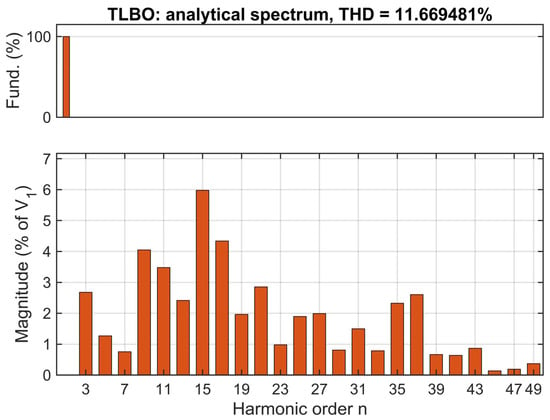
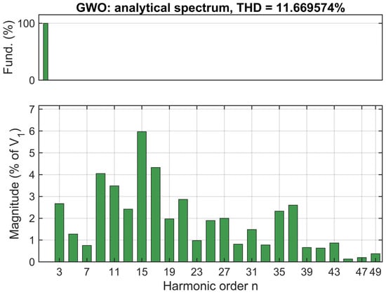
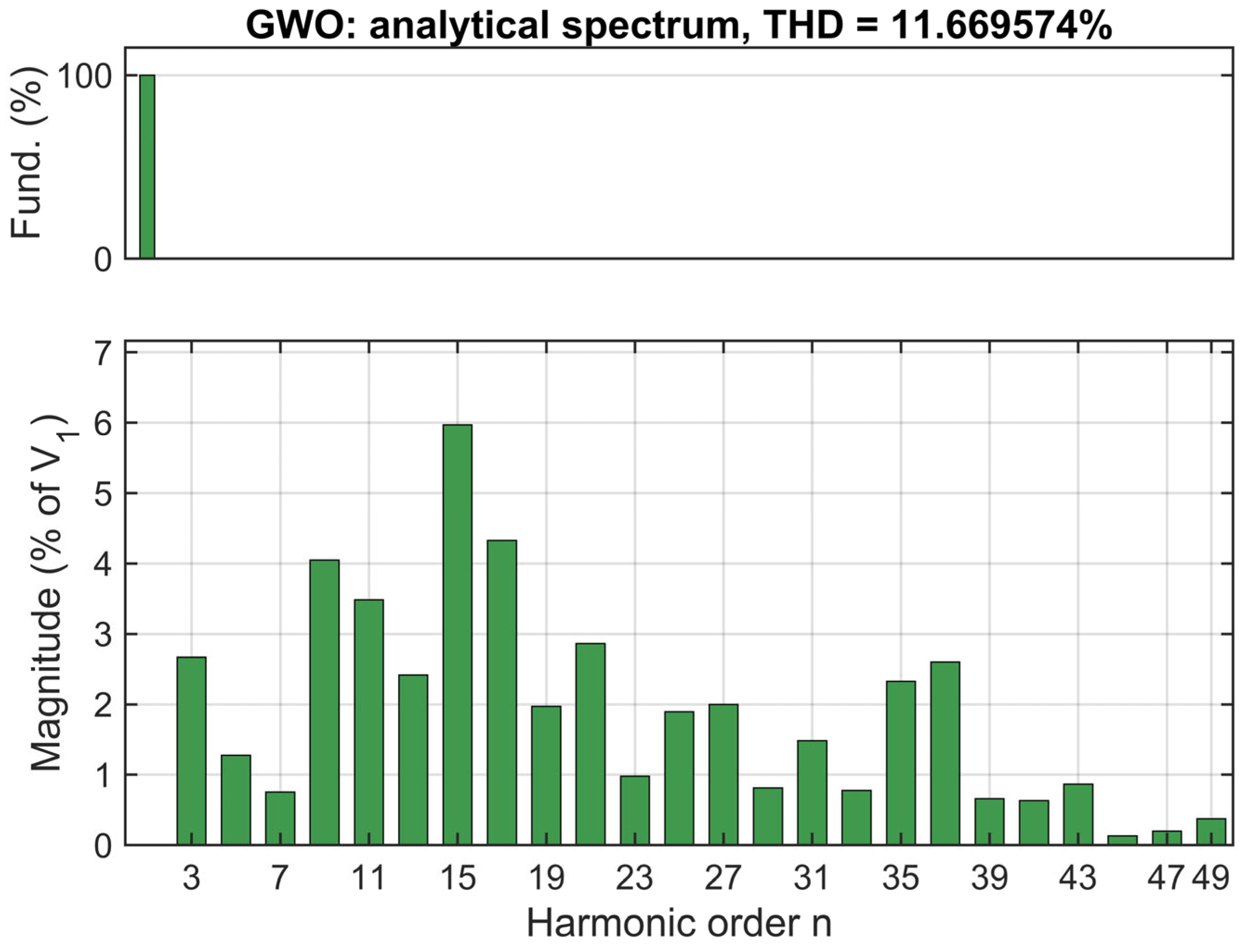
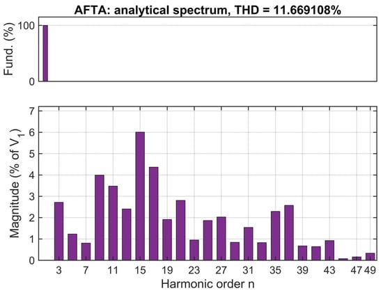
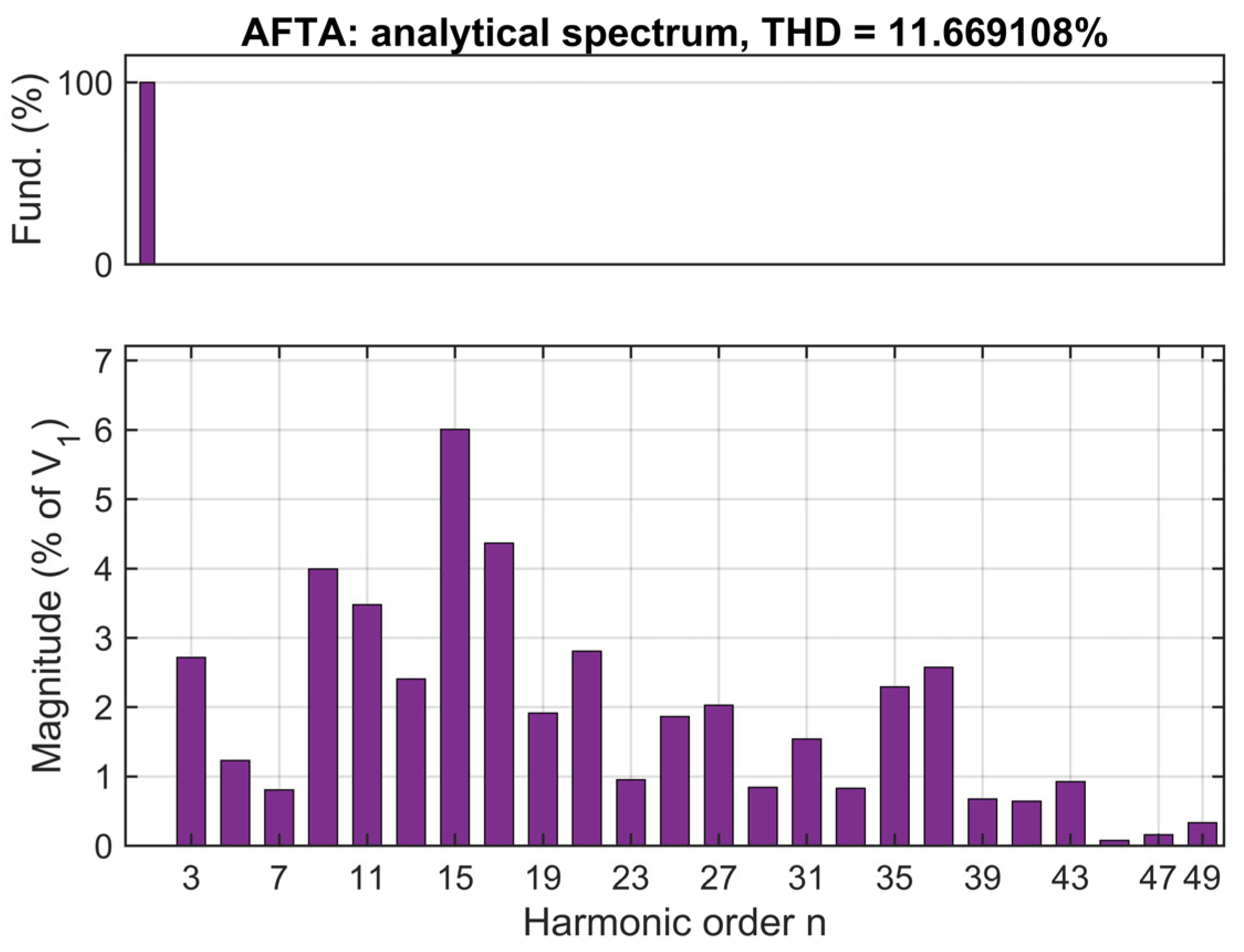
THD49 is the square root of the sum of squared non-fundamental harmonic percentages. It is neither the largest individual harmonic nor the sum of bar heights. Figure 13, Figure 14, Figure 15 and Figure 16 show the fundamental in an upper panel and harmonics 3-49 in a lower panel with a separate vertical scale. Each spectrum uses the full-precision best-J row from the new run-level dataset and is checked against its stored THD and V1.
Figure 13.
Normalized harmonic spectrum of the best DE solution (THD49 = 11.669108%).
Figure 14.
Normalized harmonic spectrum of the best TLBO solution (THD49 = 11.669481%).
Figure 15.
Normalized harmonic spectrum of the best GWO solution (THD49 = 11.669574%).
Figure 16.
Normalized harmonic spectrum of the best AFTA solution (THD49 = 11.669108%).
- DE. The best-J run used angles [10.157139264°, 31.056272134°, 58.982497976°], with V1 = 250.000000000 V and THD49 = 11.669107921%. The largest components were order 15 (6.0083% of V1) and order 17 (4.3686% of V1).
- TLBO. The best-J run used angles [10.169198282°, 30.997182416°, 59.015523158°], with V1 = 250.000039677 V and THD49 = 11.669480700%. The largest components were order 15 (5.9766% of V1) and order 17 (4.3364% of V1).
- GWO. The best-J run used angles [10.159871529°, 30.990554286°, 59.021484571°], with V1 = 249.999943671 V and THD49 = 11.669573608%. The largest components were order 15 (5.9698% of V1) and order 17 (4.3301% of V1). A smaller individual harmonic does not necessarily imply a smaller THD, which combines all included orders quadratically.
- AFTA. The best-J run used angles [10.157139280°, 31.056272110°, 58.982497987°], with V1 = 250.000000000 V and THD49 = 11.669107921%. The largest components were order 15 (6.0083% of V1) and order 17 (4.3686% of V1). Its spectrum matches DE at the displayed precision, although the measured search effort and runtime differ.
3.3. Analytical Waveform Reconstruction
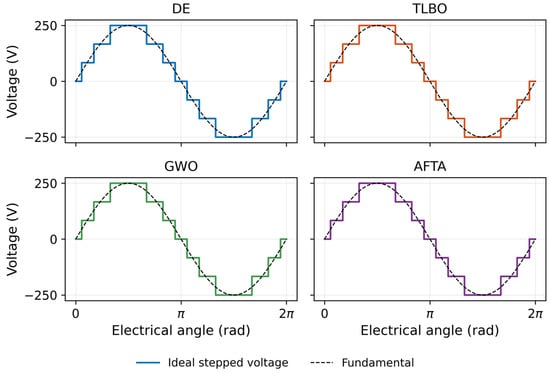
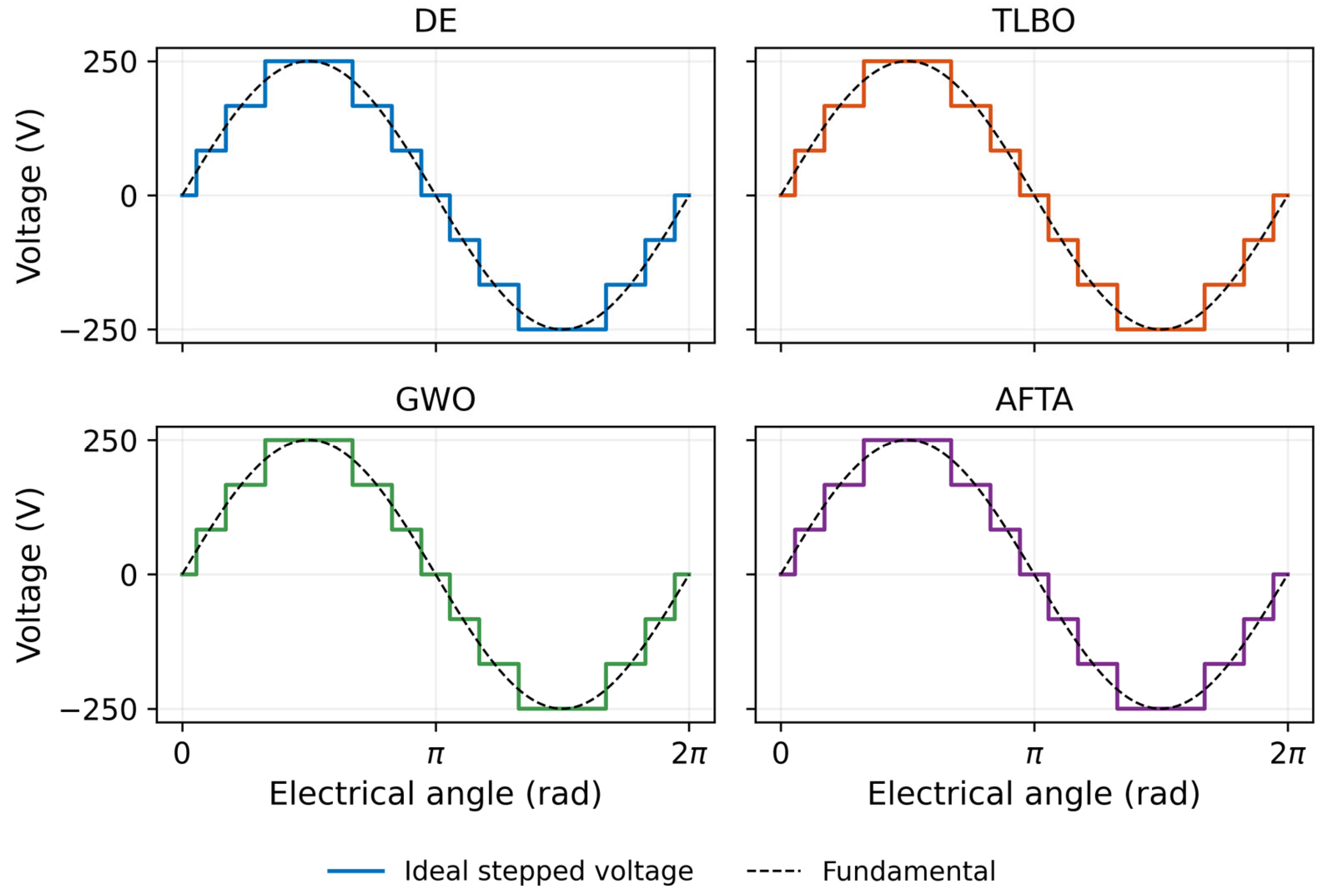
Figure 17 reconstructs the ideal output over one electrical period from each method’s full-precision best-J angles. The fundamental curve uses the corresponding calculated V1. The four stepped voltages are nearly indistinguishable at this scale, as expected from their similar harmonic spectra. This is a consistency illustration of the same analytical model, not an independent circuit simulation.
Figure 17.
Ideal stepped voltages and their fundamental components for the four best-J solutions. Solid colored lines show the ideal stepped voltage: blue for DE, orange for TLBO, green for GWO, and purple for AFTA. Black dashed lines show the corresponding fundamental components.
3.4. Per-Run Target Attainment
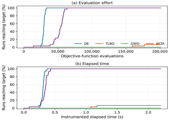
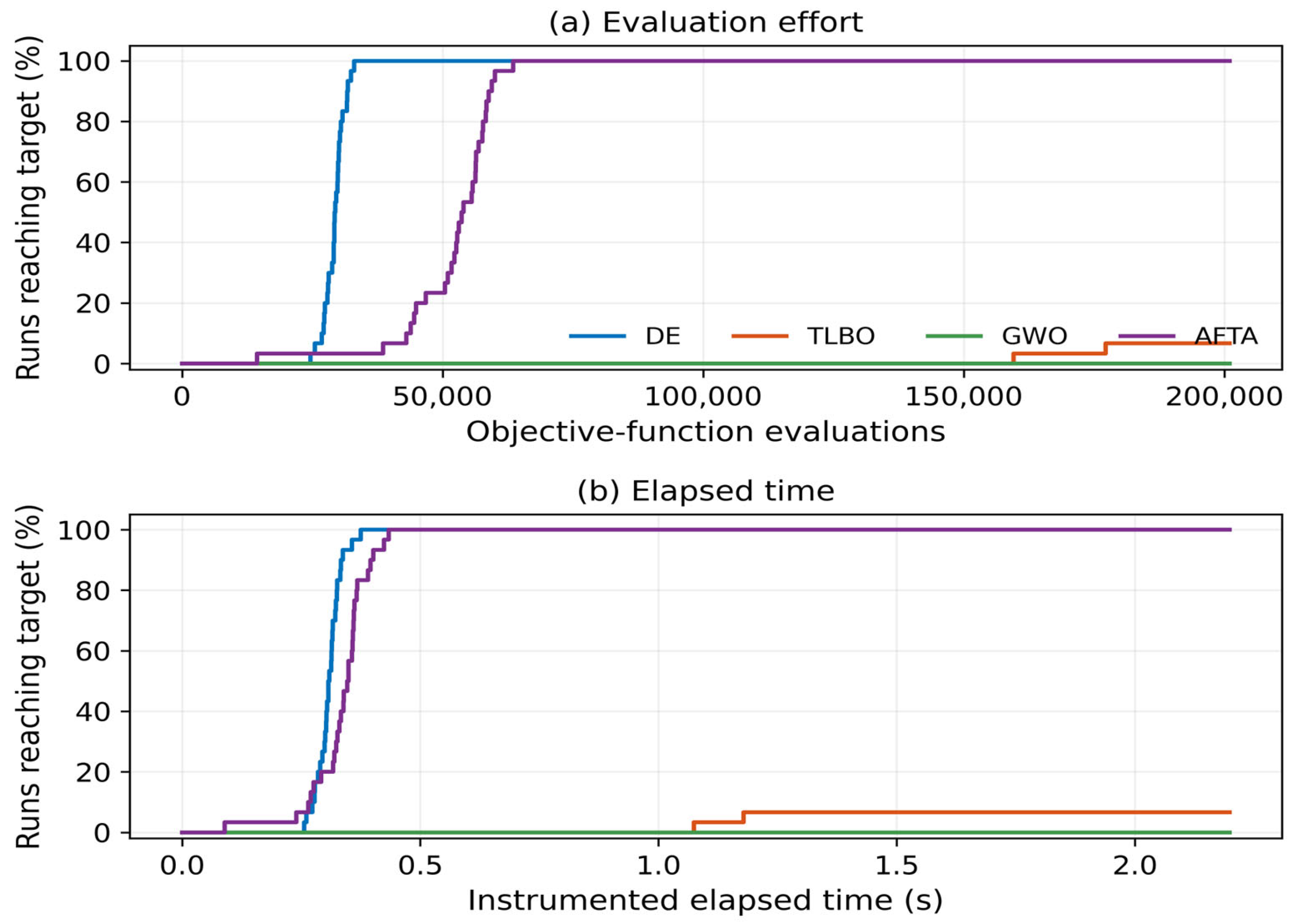
The empirical target was reached by 30/30 DE runs, 30/30 AFTA runs, 2/30 TLBO runs, and 0/30 GWO runs. Table 4 summarizes the first qualifying improvement in each run. DE’s median effort was 29,361 evaluations, compared with 53,822.5 for AFTA. Median instrumented times were 0.3079 and 0.3477 s, respectively. The two successful TLBO runs required 159,528 and 177,234 evaluations; their conditional median is not representative of the 28 unsuccessful runs. Figure 18 uses all 30 runs in each denominator and therefore preserves nonattainment.
Table 4.
First attainment of J ≤ Jref + 0.001 and |250 − V1| ≤ 0.1 V. Effort and time summaries are conditional on successful runs.
Figure 18.
Fraction of runs reaching the empirical target versus (a) objective-function evaluations and (b) instrumented elapsed time. Nonattainment is retained in the denominator.
For an independent restart interpretation, estimated runtime (ERT) in evaluations is the sum of first-hit counts for successes plus 201,000 for each failure, divided by the number of successes. The estimates are 29,283 for DE, 51,958.9 for AFTA, and 2,982,381 for TLBO; no finite estimate is available for GWO because there were no successes. This calculation is not a single observed runtime and does not treat budget-limited failures as successful hits. Conditional mean instrumented time ± SD was 0.3084 ± 0.0257 s for DE, 0.3346 ± 0.0642 s for AFTA, and 1.1261 ± 0.0737 s for the two successful TLBO runs.
3.5. Statistical Comparison and Effect Sizes
The tie-corrected Friedman statistics reject identical within-seed rankings for all four metrics (Table 5). Kendall’s W ranges from 0.8889 to 0.9613. This strong separation of ranks is not a measure of voltage quality improvement; rank effects must be interpreted alongside differences in the original units.
Table 5.
Friedman comparisons across four methods with 30 seed blocks. Holm adjustment covers the four omnibus tests.
For final J, DE, and AFTA each have lower values than TLBO and GWO after Holm adjustment across all 24 pairwise comparisons (adjusted signed-rank p = 4.47 × 10⁻⁸; |r| = 1 for these pairs). DE and AFTA are tied at the 10−9 analysis resolution (p = 1, r = 0); this is not a general equivalence test. TLBO versus GWO is not significant after adjustment (p = 0.9113). The same rejection pattern holds for THD and absolute voltage error, and the sign test sensitivity analysis agrees. Table 6 reports the primary endpoint in its original units.
Table 6.
Paired final-J comparisons. Δ is the median of A − B; r is rank-biserial correlation. Both adjusted p columns use their respective 24-comparison Holm families.
All full-budget runtime pairs remain distinguishable after adjustment (Table 7). AFTA has the lowest mean runtime; the TLBO-GWO median paired difference is −0.03125 s, with adjusted signed-rank p = 3.60 × 10⁻⁵ and r = −0.8624. Exact sign tests support the same pairwise runtime conclusions. These tests concern the separate timing passes on the reported machine and do not establish intrinsic algorithmic complexity or an online control guarantee.
Table 7.
Paired full-budget runtime comparisons without detailed logging. Δ is the median of A − B in seconds; Holm families are defined as in Table 6.
4. Discussion
Figure 13, Figure 14, Figure 15 and Figure 16 allow comparison of the distribution of harmonic components of the best runs. In the four profiles, order 15 predominates, followed mainly by 17, 9, and 11. DE and AFTA coincide at the represented scale. TLBO and GWO produce small variations that redistribute the harmonic content. The absence of even orders derives from the ideal symmetry of the model and does not constitute an experimental verification of the commutation.
The best-solution THD ranges from 11.6691079213% for DE/AFTA to 11.6695736079% for GWO: a separation of 0.0004656866 percentage points, or 0.0039908% of the best THD. At a common 250 V peak fundamental, this corresponds to an approximately 0.0008232 V difference in truncated harmonic RMS magnitude. This calculation quantifies the small electrical scale of the numerical difference; it does not demonstrate an observable improvement in a physical converter. The nearly identical best spectra must be distinguished from the distributions across all 30 runs.
Statistical separation is strongest between DE/AFTA and TLBO/GWO in the tested final metrics, but its engineering magnitude remains small. All final fundamental voltage errors are below 0.1 V, and the largest observed error is 0.0006238 V. AFTA minimizes full-budget runtime among these implementations, whereas DE has a smaller median evaluation count and instrumented time to the empirical target. Selection therefore depends on whether the relevant cost is completing the full budget or attaining a specified numerical precision.
The strict success rate is 100% for DE and AFTA, 6.7% for TLBO, and 0% for GWO. This indicator depends on the threshold Jref + 0.001 and does not equate to an electrical acceptance test of a physical inverter. GWO meets the voltage tolerance but does not reach the J threshold. Therefore, the result describes the numerical accuracy obtained under the selected criterion and should be interpreted along with THD and voltage error.
4.1. Relationship with Previous Converter Studies
The reviewed literature allows the comparison to be situated in two related lines. The systematic review by Sánchez-Vargas et al. [1] shows that the combination of CHB topology, seven levels, and evolutionary methods constitutes a recurring case study in THD minimization. Therefore, the configuration selected in this work is not proposed as a new topology, but rather as a sufficiently documented scenario to compare search strategies.
The study by Sánchez Vargas et al. [2] applied DE to a seven-level CHB, performed a modulation index sweep, and experimentally validated two sets of angles. Their results show that the value of THD and the amplitude of the fundamental depend on the reference condition used. This observation justifies that, in the present protocol, all algorithms share a fixed reference of 250 V peak and the same cost function; consequently, the THD values of both works should not be directly compared if the formulation, modulation index, or selection criteria change.
On the other hand, the review by Gómez Díaz et al. [3] documents the use of TLBO in electronics and notes, as a characteristic of its basic version, the absence of specific control parameters comparable to F and CR of DE. The subsequent work by Gómez Díaz et al. [4] directly studied the minimization of THD in a seven-level CHB and compared TLBO with GA, DE, and PSO through a modulation index sweep. That precedent supports the inclusion of TLBO, but the present study uses a different protocol: a fixed reference of the fundamental, a common budget of evaluations, 30 seeds per algorithm, and the incorporation of GWO and AFTA.
The comparison adds a distinction between final electrical quality, seed-to-seed numerical behavior, and computational effort. The inclusion of GWO and AFTA is informative because similar best spectra coexist with different attainment rates and timing distributions under one shared formulation. This is evidence about the implemented procedures at a fixed operating point, not a demonstration that any algorithm family is universally superior. Establishing broader robustness requires additional experiments across populations, parameters, and voltage references.
4.2. Scope and Limits of the Comparison
The coincidence between DE and AFTA demonstrates the repetition of the best point found within the experiment, but it does not certify that it is the global minimum of the function. To establish a property of optimality, an additional analysis of the domain and feasible solutions would be necessary. Likewise, the weighted function depends on λV and the reference; changing either of these elements can modify the search geometry and the relative order of performance.
The 30-seed repetitions characterize stochastic variability only at Np = 1000 and the stated operator settings. They do not establish robustness to population size or hyperparameters. No population-size sensitivity experiment is included, and no claim is made that the observed ordering would persist for smaller populations or separately tuned methods. A limited follow-up should vary population size while retaining the same total evaluation budget, electrical objective, and paired seeds, and compare attainment rates, evaluation counts, and runtime while documenting any incomplete TLBO cycle and re-scaled coefficient schedule. This separates the present baseline conclusions from the additional evidence required for configuration robustness.
The reported THD corresponds to voltage and is truncated at the 49th harmonic. It does not describe the THD of current in an RL load nor the behavior of a switched source. The filtering associated with an inductive load can modify the current without changing the voltage spectrum used here. Dead time, semiconductor drops, or source imbalances are also not included. Therefore, the analytical values should not be interpreted as measurements of a prototype or as a comprehensive assessment of power quality compliance [40].
Runtime comparisons apply to the supplied MATLAB code and machine. The detailed-logging passes averaged 2.0037, 1.3679, 1.3804, and 1.1926 s for DE, TLBO, GWO, and AFTA, respectively, while the separate non-detailed passes supplied the runtimes in Table 3. Because the passes occurred at different instants, their difference is not an isolated measurement of logging overhead; execution order, system load, and frequency changes can contribute. The time-to-target values belong only to the instrumented passes. No real-time controller deadline or intrinsic implementation-independent complexity advantage follows from these timings.
5. Conclusions
Four population-based metaheuristic implementations were evaluated for switching angle optimization of an ideal seven-level single-phase CHB inverter. The protocol paired 30 seeds across methods, used 201,000 evaluations per run, and combined voltage THD through order 49 with absolute fundamental voltage error relative to 250 V peak. Run-level improvement events and separate timing passes distinguish final solution quality, target attainment effort, and full-budget computational cost.
DE and AFTA attained the same displayed best THD49 of 11.6691079%, with angles near [10.157139°, 31.056272°, 58.982498°], and reached the empirical target in all 30 runs. Their median evaluation counts to target were 29,361 and 53,822.5, respectively. AFTA had the lowest mean full-budget runtime (1.2354 s), compared with 2.0742 s for DE; DE had the shorter median instrumented time to target (0.3079 versus 0.3477 s). These metrics answer different computational questions and do not establish global optimality.
After adjustment across 24 paired comparisons, DE and AFTA differed from TLBO and GWO in final J, THD and absolute voltage error, but DE and AFTA were indistinguishable at the declared statistical resolution. TLBO and GWO were not separated in those final electrical/objective metrics. Their target attainment rates were 2/30 and 0/30 under the selected numerical criterion. All four methods remained within the fundamental voltage tolerance; statistical separation therefore does not imply a practically important electrical improvement.
The spectral analysis shows that the best solutions are electrically similar and that the 15th harmonic dominates in all cases. The small variations between bars do not directly translate into an improvement in THD, as this metric quadratically integrates all the included orders. The comparison should be based on the combined indicators and not on an isolated component or the visual aspect of an enlarged axis.
NR remains as a deterministic reference. Its quantitative evaluation requires defining initial conditions, accounting for failures, and including the cost of the linear system and the Jacobian. The combinations with neural networks and metaheuristics constitute precedents for that extension [4,9,28]. It is also pertinent to study the effect of population size and budget, maintaining a protocol defined before observing the results.
The findings are conditional on the analytical model, the 250 V reference, Np = 1000, and the stated algorithm settings. They support comparisons of the supplied implementations at this fixed configuration, not population-independent or optimally tuned algorithm rankings. Population-size, hyperparameter, and operating condition sensitivity remain untested limitations. Further numerical work can examine those factors and extend the ideal model to source mismatch, nonideal switching, and load dynamics. The current conclusions concern analytical simulation and optimizer behavior; they are not claims about prototype performance.
Supplementary Materials
The following supporting information can be downloaded at: https://www.mdpi.com/article/10.3390/a19110905/s1, Reproducibility_CHB_minor_revision.zip: reproducibility package containing the executed MATLAB source, original run-level data, statistical outputs, computational environment, and reproduction instructions. Appendix A identifies the principal files and commands.
Author Contributions
Conceptualization, J.A.A. and S.E.D.L.-A.; methodology, S.A.P.F., J.A.A., S.E.D.L.-A., M.P.-S. and V.H.O.P.; software, S.A.P.F. and R.E.L.-P.; validation, S.A.P.F., S.E.D.L.-A., M.P.-S., V.H.O.P., H.A.-P. and P.J.G.-R.; formal analysis, S.A.P.F., J.A.A., S.E.D.L.-A., M.P.-S., V.H.O.P., H.A.-P., P.J.G.-R. and R.E.L.-P.; investigation, S.A.P.F.; resources, M.P.-S., V.H.O.P., H.A.-P. and P.J.G.-R.; data curation, S.A.P.F., M.P.-S., V.H.O.P., P.J.G.-R. and R.E.L.-P.; writing—original draft, S.A.P.F.; writing—review and editing, J.A.A., S.E.D.L.-A., M.P.-S., V.H.O.P., H.A.-P., P.J.G.-R. and R.E.L.-P.; visualization, S.A.P.F. and R.E.L.-P.; supervision, J.A.A. and S.E.D.L.-A.; project administration, J.A.A. and S.E.D.L.-A.; funding acquisition, H.A.-P. and P.J.G.-R. All authors have read and agreed to the published version of the manuscript.
Funding
This research received no external funding.
Data Availability Statement
The data and code supporting the reported tables and figures are supplied in Reproducibility_CHB_minor_revision.zip. The original measurements are retained alongside instructions for regenerating figures and rerunning the study; see Appendix A.
Acknowledgments
ChatGPT (OpenAI, GPT-6) assisted in organizing the structure of the document. The authors provided the results of the MATLAB runs. During the review process, independent calculations in Python were used to verify numerical consistency and prepare the combined analytical figures. No experimental measurements were generated. The authors remain responsible for verifying the code, analyses, references, and the final manuscript.
Conflicts of Interest
The authors declare no conflicts of interest.
Abbreviations
The following abbreviations are used in this manuscript:
| AFTA | Ali Baba and the Forty Thieves Algorithm |
| CHB | Cascaded H-bridge |
| DE | Differential Evolution |
| GWO | Grey Wolf Optimizer |
| IQR | Interquartile range |
| NR | Newton–Raphson |
| RMS | Root mean square |
| SHE | Selective harmonic elimination |
| THD | Total harmonic distortion |
| TLBO | Teaching-Learning-Based Optimization |
Appendix A
The supplementary archive Reproducibility_CHB_minor_revision.zip contains RE-ADME_REPRODUCIBILITY.md, the unchanged executed source CHB_UNIFICADO_usado.m, an identical copy named CHB_UNIFICADO.m for direct MATLAB invocation, configuracion_y_entorno.mat, entorno_y_protocolo.txt and princi-pal_250V/. The latter includes estudio.mat, resultados_corridas.csv, convergen-cia_por_corrida.csv, mejoras_evaluacion_exacta.csv, estadistica_Friedman.csv, estadisti-ca_pares_Wilcoxon_Holm.csv, resumen_comparativo.csv, resumen_espectros.csv and the per-method harmonic and waveform data. SHA256SUMS.txt records file checksums. Only the principal 250 V case is supplied; optional sensitivity modes are not evidence that additional experiments were run.
For figure regeneration without optimization, extract the archive, set its root as the MATLAB current folder, and run CHB_UNIFICADO (‘graficas’, fullfile(pwd, ‘principal_250V’, ‘estudio.mat’)). To recompute the statistical tables from saved runs without new optimization, run reproducir_estadisticas. For a new execution of the full principal study, run CHB_UNIFICADO(‘principal’); this creates a separate timestamped results folder and regenerates statistical outputs as well as figures. The reference CSV files retain the originally measured runtimes, which must be used when checking the published timing statistics; fresh timings are machine- and session-dependent. verificar_resultados.py independently checks the saved electrical results, first-hit events and Friedman statistics, while figuras_articulo.py regenerates the combined waveform and target attainment figures. The README lists dependencies, commands and the mapping of files to Table 3, Table 4, Table 5, Table 6 and Table 7 and Figure 9, Figure 10, Figure 11, Figure 12, Figure 13, Figure 14, Figure 15, Figure 16, Figure 17 and Figure 18, including the global Holm columns used in the manuscript.
GitHub link: https://github.com/m25ce069-ui/Calculation-of-Switching-Angles-in-a-Cascaded-Multilevel-Converter-Using-a-Bio-Inspired-Algorithm (accessed on 13 October 2026).
References
- Sánchez-Vargas, O.; De León-Aldaco, S.E.; Aguayo-Alquicira, J.; López-Núñez, A.R. Evolutionary metaheuristic methods applied to minimize the THD in inverters: A systematic review. Eur. J. Electr. Eng. 2021, 23, 237–245. [Google Scholar] [CrossRef] [Scilit]
- Sánchez Vargas, O.; De León Aldaco, S.E.; Aguayo Alquicira, J.; Vela Valdés, L.G.; Mina Antonio, J.D. Differential evolution applied to a multilevel inverter—A case study. Appl. Sci. 2022, 12, 9910. [Google Scholar] [CrossRef] [Scilit]
- Gómez Díaz, K.Y.; De León Aldaco, S.E.; Aguayo Alquicira, J.; Ponce-Silva, M.; Olivares Peregrino, V.H. Teaching-Learning-Based Optimization algorithm applied in electronic engineering: A survey. Electronics 2022, 11, 3451. [Google Scholar] [CrossRef] [Scilit]
- Gómez Díaz, K.Y.; de León Aldaco, S.E.; Aguayo Alquicira, J.; Vela Valdés, L.G. THD minimization in a seven-level multilevel inverter using the TLBO algorithm. Eng 2023, 4, 1761–1786. [Google Scholar] [CrossRef] [Scilit]
- Storn, R.; Price, K. Differential evolution—A simple and efficient heuristic for global optimization over continuous spaces. J. Glob. Optim. 1997, 11, 341–359. [Google Scholar] [CrossRef] [Scilit]
- Mirjalili, S.; Mirjalili, S.M.; Lewis, A. Grey Wolf Optimizer. Adv. Eng. Softw. 2014, 69, 46–61. [Google Scholar] [CrossRef] [Scilit]
- Rao, R.V.; Savsani, V.J.; Vakharia, D.P. Teaching–Learning-Based Optimization: A novel method for constrained mechanical design optimization problems. Comput.-Aided Des. 2011, 43, 303–315. [Google Scholar] [CrossRef] [Scilit]
- Braik, M.; Ryalat, M.H.; Al-Zoubi, H. A novel meta-heuristic algorithm for solving numerical optimization problems: Ali Baba and the Forty Thieves. Neural Comput. Appl. 2022, 34, 409–455. [Google Scholar] [CrossRef] [Scilit]
- Marín-Reyes, M.; Aguayo-Alquicira, J.; De León-Aldaco, S.E. Calculation of optimal switching angles for a multilevel inverter using NR, PSO, and GA—A comparison. Eur. J. Electr. Eng. 2020, 22, 349–355. [Google Scholar] [CrossRef] [Scilit]
- Padmanaban, S.; Dhanamjayulu, C.; Khan, B. Artificial neural network and Newton Raphson (ANN-NR) algorithm based selective harmonic elimination in cascaded multilevel inverter for PV applications. IEEE Access 2021, 9, 75058–75070. [Google Scholar] [CrossRef] [Scilit]
- Lopez, A.R.; Cortes, C.J.; Munoz, M.G.; Verdin, J.A.; Perez, J.F.; Vazquez, G.; Sosa, J.M.; Aguayo, J.; Aldaco, S.D.L. Harmonic mitigation in a multilevel inverter with the Newton Raphson method and the particle swarm optimization. In Proceedings of the 2021 IEEE International Autumn Meeting on Power, Electronics and Computing (ROPEC), Ixtapa, Mexico, 10–12 November 2021; pp. 1–6. [Google Scholar] [CrossRef] [Scilit]
- Djafer, L.; Taleb, R.; Toubal Maamar, A.E.; Mehedi, F.; Mostefaoui, S.A.; Rekmouche, H. Analysis and experimental implementation of SHEPWM based on Newton-Raphson algorithm on three-phase inverter using dSPACE 1104. In Proceedings of the 2023 2nd International Conference on Electronics, Energy and Measurement (IC2EM), Medea, Algeria, 28–29 November 2023; pp. 1–6. [Google Scholar] [CrossRef] [Scilit]
- Biswas, S.D.; Das, B.; Nandi, C. Optimized switching angle control using Newton-Raphson method for THD reduction in cascaded H-bridge multilevel inverters. In Proceedings of the 2024 IEEE Silchar Subsection Conference (SILCON 2024), Agartala, India, 15–17 November 2024. [Google Scholar] [CrossRef] [Scilit]
- Thiyagarajan, S.; Anbukumar, K. Novel implementation method of selective harmonic elimination on a low cost FPGA controller for V2G application. In Proceedings of the 2025 IEEE Energy Conversion Congress and Exposition Asia (ECCE-Asia), Bengaluru, India, 11–14 May 2025. [Google Scholar] [CrossRef] [Scilit]
- Ahmad, M.F.; Isa, N.A.M.; Lim, W.H.; Ang, K.M. Differential evolution: A recent review based on state-of-the-art works. Alex. Eng. J. 2022, 61, 3831–3872. [Google Scholar] [CrossRef] [Scilit]
- Wang, J.; Shang, S.; Jing, H.; Zhu, J.; Song, Y.; Li, Y.; Deng, W. A novel multistrategy-based differential evolution algorithm and its application. Electronics 2022, 11, 3476. [Google Scholar] [CrossRef] [Scilit]
- Stanovov, V.; Kazakovtsev, L.; Semenkin, E. Crossover rate sorting in adaptive differential evolution. Algorithms 2023, 16, 133. [Google Scholar] [CrossRef] [Scilit]
- Huang, Y.; Qian, X.; Song, W. Improving dual-population differential evolution based on hierarchical mutation and selection strategy. Electronics 2024, 13, 62. [Google Scholar] [CrossRef] [Scilit]
- Saad, A.; Engelbrecht, A.P.; Khan, S.A. An analysis of differential evolution population size. Appl. Sci. 2024, 14, 9976. [Google Scholar] [CrossRef] [Scilit]
- Ma, Y.; Li, Y.; Yong, L. Teaching–Learning-Based Optimization algorithm with stochastic crossover self-learning and blended learning model and its application. Mathematics 2024, 12, 1596. [Google Scholar] [CrossRef] [Scilit]
- Hubálovský, Š.; Hubálovská, M.; Matoušová, I. A new hybrid particle swarm optimization–Teaching–Learning-Based Optimization for solving optimization problems. Biomimetics 2024, 9, 8. [Google Scholar] [CrossRef] [Scilit]
- Lu, S.; Liu, D.; Li, D.; Shao, X. Enhanced Teaching–Learning-Based Optimization algorithm for the mobile robot path planning problem. Appl. Sci. 2023, 13, 2291. [Google Scholar] [CrossRef] [Scilit]
- Lei, D.; Zhang, J.; Liu, H. An adaptive two-class Teaching–Learning-Based Optimization for energy-efficient hybrid flow shop scheduling problems with additional resources. Symmetry 2024, 16, 203. [Google Scholar] [CrossRef] [Scilit]
- Li, J.; Guo, X.; Zhang, Q. Multi-strategy discrete Teaching-Learning-Based Optimization algorithm to solve no-wait flow-shop-scheduling problem. Symmetry 2023, 15, 1430. [Google Scholar] [CrossRef] [Scilit]
- Makhadmeh, S.N.; Al-Betar, M.A.; Abu Doush, I.; Awadallah, M.A.; Kassaymeh, S.; Mirjalili, S.; Abu Zitar, R. Recent advances in Grey Wolf Optimizer, its versions and applications: Review. IEEE Access 2024, 12, 22991–23028. [Google Scholar] [CrossRef] [Scilit]
- Al-Dmour, A.S.; Al-Majali, H.D.; Al-Majali, Z.S. Staircase modulation using GWO technique for CHB-MLI with symmetrical and asymmetrical mode. Int. J. Eng. Trends Technol. 2021, 69, 71–80. [Google Scholar] [CrossRef] [Scilit]
- Srilekha, B.; Babu, B.G.; Priya, H.; Kapoor, R.; Sobhana, O. Harmonic elimination using PSO and GWO in cascaded H-bridge multilevel inverter. In Proceedings of the 2023 9th International Conference on Electrical Energy Systems (ICEES), Chennai, India, 23–25 March 2023; pp. 294–299. [Google Scholar] [CrossRef] [Scilit]
- Kala, P.; Jately, V.; Sharma, A.; Joshi, J.; Kotb, H.; AboRas, K.M.; Elrashidi, A. GWO-NR hybrid method for selective harmonic elimination in multilevel inverter for distributed energy systems. IEEE Access 2024, 12, 27957–27972. [Google Scholar] [CrossRef] [Scilit]
- Hussein, T.A.; Ishak, D.; Tarnini, M. A three-phase multilevel inverter synthesized with 31 levels and optimal gating angles based on the GA and GWO to supply a three-phase induction motor. Energies 2024, 17, 1267. [Google Scholar] [CrossRef] [Scilit]
- Ürgün, S.; Yiğit, H.; Mirjalili, S. Investigation of recent metaheuristics based selective harmonic elimination problem for different levels of multilevel inverters. Electronics 2023, 12, 1058. [Google Scholar] [CrossRef] [Scilit]
- Bhatt, B.; Sharma, H.; Arora, K.; Joshi, G.P.; Shrestha, B. Levy flight-based improved Grey Wolf Optimization: A solution for various engineering problems. Mathematics 2023, 11, 1745. [Google Scholar] [CrossRef] [Scilit]
- Braik, M. Enhanced Ali Baba and the Forty Thieves algorithm for feature selection. Neural Comput. Appl. 2023, 35, 6153–6184. [Google Scholar] [CrossRef] [Scilit]
- Rehman, K.U.; Sajid, I.; Lu, S.-D.; Ahmad, S.; Liu, H.-D.; Bakhsh, F.I.; Tariq, M.; Sarwar, A.; Lin, C.-H. Fast tracking of maximum power in a shaded photovoltaic system using Ali Baba and the Forty Thieves (AFT) algorithm. Processes 2023, 11, 2946. [Google Scholar] [CrossRef] [Scilit]
- Al-Hiary, H.; Braik, M.; Al-Betar, M.A. Optimizing connection weights in neural networks using Ali Baba and the Forty Thieves algorithm. In Proceedings of the 2023 24th International Arab Conference on Information Technology (ACIT), Ajman, United Arab Emirates, 6–8 December 2023; pp. 1–7. [Google Scholar] [CrossRef] [Scilit]
- Rushdi, H.; Al-Naima, F. Estimation of PV cell equivalent circuit parameters based on Ali Baba and the Forty Thieves algorithm. In Proceedings of the 2022 International Conference on Technology and Policy in Energy and Electric Power (ICT-PEP), Jakarta, Indonesia, 18–20 October 2022. [Google Scholar] [CrossRef] [Scilit]
- Sahu, B.; Pani, S.; Panigrahi, A.; Pati, A.; Patro, R.R.; Ravindra, J.V.R. A hybrid particle swarm optimization with binary Ali Baba and the Forty Thieves algorithm for feature selection. In Proceedings of the 2024 3rd Odisha International Conference on Electrical Power Engineering, Communication and Computing Technology (ODICON), Bhubaneswar, India, 8–9 November 2024; pp. 1–6. [Google Scholar] [CrossRef] [Scilit]
- Friedman, M. The use of ranks to avoid the assumption of normality implicit in the analysis of variance. J. Am. Stat. Assoc. 1937, 32, 675–701. [Google Scholar] [CrossRef]
- Wilcoxon, F. Individual comparisons by ranking methods. Biom. Bull. 1945, 1, 80–83. [Google Scholar] [CrossRef] [Scilit]
- Holm, S. A simple sequentially rejective multiple test procedure. Scand. J. Stat. 1979, 6, 65–70. [Google Scholar]
- IEEE Std 519-2022; IEEE Standard for Harmonic Control in Electric Power Systems. IEEE: New York, NY, USA, 2022.

Disclaimer/Publisher’s Note: The statements, opinions and data contained in all publications are solely those of the individual author(s) and contributor(s) and not of MDPI and/or the editor(s). MDPI and/or the editor(s) disclaim responsibility for any injury to people or property resulting from any ideas, methods, instructions or products referred to in the content. |
© 2026 by the authors. Licensee MDPI, Basel, Switzerland. This article is an open access article distributed under the terms and conditions of the Creative Commons Attribution (CC BY) license.