


Abstract
Physics-informed neural networks (PINNs) have recently emerged as an effective surrogate to classical numerical methods for solving partial differential equations (PDEs) in a wide range of physical systems. When augmented with supervised data, PINN performance can depend strongly on the quality and characteristics of the training data; however, the influence of the numerical method used to generate that data remains largely unexplored. In this study, we investigate how training data generated by finite difference method (FDM) and finite element method (FEM) solvers affects PINN training and predictive accuracy, particularly in solving the one-dimensional heat equation under conditions relevant to laser–tissue interactions. A supervised data loss term is incorporated, and models trained on FDM- and FEM-generated temperature fields under identical physical conditions are compared to assess differences in convergence and accuracy. The results demonstrate that, under controlled one-dimensional diffusion settings, the numerical solver used for data generation produces a quantifiable, resolution-dependent effect on hybrid PINN performance: FDM-generated training data yields the lowest error across most tested resolutions, an advantage that narrows and becomes indistinguishable only at the finest resolution considered, providing practical guidance for selecting a data-generating solver in biological heat transfer applications.
Keywords:
FDM; FEM; heat equation; machine learning; numerical methods; PAC1D; PDE; pdepe; PINN; skin model 1. Introduction
Modeling heat transfer in biological tissue is critical for applications in medicine and defense, including burn diagnostics and laser safety, as even moderate laser-induced heating can cause rapid tissue damage [1]. Partial differential equations (PDEs) provide a well-established mathematical framework to describe heat diffusion in tissue, allowing for the representation of multiple physical properties and tissue layers; however, analytical solutions are often intractable, and obtaining high-resolution numerical solutions can be computationally expensive [2]. Recent developments in machine learning have produced several surrogates to traditional numerical methods in the form of deep neural networks (DNNs) [3,4,5]. Typically, the predictive capability of a DNN hinges on the availability of high-quality data; however, this dependence has been alleviated by the emergence of physics-informed neural networks (PINNs) [6]. In this work, we investigate PINNs as surrogate models for solving the one-dimensional heat diffusion equation, with a focus on how the choice of numerical solver used to generate training data affects model performance.
1.1. Physics-Informed Neural Networks
PINNs are deep neural networks that incorporate the governing PDE directly into the training process. Rather than relying on high-resolution meshes, PINNs embed the residual of the underlying PDE into the loss function using automatic differentiation, enabling the network to approximate a continuous solution across the spatiotemporal domain [6]. Boundary and initial conditions are likewise enforced through additional penalty terms, producing a mesh-free surrogate that respects physical constraints. As a result, PINNs offer a comparatively strong advantage to classical numerical solvers in their flexibility for domain representation. Additionally, once trained, a PINN can rapidly output a prediction at any point in the domain. However, purely physics-based PINNs can struggle when physical knowledge is limited, which is not uncommon in real, complex use cases [7].
In scenarios where detailed experimental measurements are limited or unavailable, even sparse numerical data can serve as a source of supervision for PINNs [8]. Incorporating supervised data into the loss function can improve stability, predictive accuracy, and training time, while not demanding extremely fine meshes, as some physical knowledge is available [9]. This hybrid training strategy blends data-driven learning with embedded physical structure, potentially yielding models that retain physical consistency while benefiting from data-guided optimization.
1.2. Finite Difference Method and Finite Element Method
The two primary numerical methods investigated in this study are the finite difference method (FDM) and finite element method (FEM). FDM discretizes the domain of a PDE into a regular grid and approximates spatial and temporal derivatives using differences between neighboring points [10]. By assembling these approximations across the entire domain, the governing PDE is transformed into a system of algebraic equations that can be solved numerically. FDM is straightforward and computationally efficient for problems defined on structured grids; however, it may procure greater error from irregular geometries such as those encountered at interfaces between layers of skin tissue [10].
FEM differs from FDM in its approach to spatial discretization. Instead of a regular grid, FEM partitions the domain into a collection of elements and approximates the solution using basis functions that are defined locally over each element [11]. As with FDM, the contributions from all elements are assembled into a global system of algebraic equations that can be solved numerically. By allowing non-uniform elements, FEM is well suited for problems involving complex geometries and heterogeneous material properties; however, this flexibility typically comes at a higher computational cost compared to FDM [12].
1.3. Significance of the Work
To the best of our knowledge, although FDM and FEM are well-established numerical techniques for solving PDEs, limited attention has been given to isolating the impact of source data topology on the training and predictive performance of hybrid PINNs [13]. Because supervised PINNs incorporate numerical solutions from different methods directly into the loss function, local error distribution and boundary treatment may implicitly shape the loss landscape encountered during training. To investigate this effect, a controlled comparison is performed in which PINNs are trained under identical physical conditions and network architectures, differing only in the numerical source of supervised temperature data. Convergence behavior and predictive accuracy are evaluated for a three-layer skin model across a range of spatial and temporal discretization resolutions, to assess how solver choice affects hybrid physics-informed learning.
The primary contributions of this work are thus as follows: a systematic, quantitative comparison of FDM- and FEM-generated supervisory data in hybrid PINN training across a range of spatiotemporal resolutions; an analysis of convergence and predictive performance under controlled physical conditions; and an evaluation of how solver-induced effects on PINN accuracy depend on training-data resolution, together with a demonstration that biasing supervised-point sampling toward regions of known inter-solver disagreement improves training stability. The remainder of the paper presents the skin model, the governing PDE, the implementation of numerical methods, the formulation of the PINN, the experimental setup, the results, and the surrounding discussion and conclusions.
2. Materials and Methods
2.1. Skin Configurations
In this study, a three-layer human skin configuration (epidermis, dermis, and fat) was considered, selected as an anatomically representative configuration examined in this line of prior work [14,15]. The material properties of relevance are thermal conductivity, density, and specific heat capacity, as these determine the thermal diffusivity used in the governing heat diffusion equation. For each skin layer, those values are shown below as , , and , respectively.
A heat source term representing the laser exposure was applied for 0.5 s and then switched off for 0.5 s. The irradiance is given as
This expression represents the nominal irradiance incident on the skin surface. PAC1D simulates an accurate representation of the laser dose in tissue using the wavelength-dependent optical tissue properties of each layer, which account for both attenuation and anisotropic scattering. This source term is reflected in the resulting training data used throughout this study though not described in detail here.
The skin model possesses a total depth of 0.012 m, with homogeneous Neumann boundary conditions and resting initial temperature K. In the multilayer configuration, thermal diffusivity is piecewise constant with discontinuities at the tissue layer interfaces. These interfaces are the regions along the spatial domain, denoted by x in meters, where predictive models are expected to struggle the most [16]. The exact points of discontinuity for this multilayer configuration are highlighted in the piecewise function definition below.
2.2. Governing Partial Differential Equation
With the skin configuration defined, the governing PDE representing this process can be expressed generally as a spatial and temporal function of temperature, , in one dimension as
for a source term Q. For this problem, our governing PDE, together with boundary and initial conditions, is
where the thermal properties , , and are as defined in Table 1and vary with depth according to the skin layer at x, x is the spatial depth in meters, t is the time in seconds, T is the temperature in Kelvin, is the initial temperature, and is as defined in Equation (1). is the resulting source term, where the irradiance governs the laser dosage delivered to the skin surface.
Table 1.
Thermophysical properties of human skin layers [15].
2.3. Numerical Method Implementations
The reference FDM solution was generated using Python Ablation Code 1-Dimension (PAC1D) v4.1, the Air Force Research Laboratory’s proprietary finite difference–based numerical solver [17], adopted here as a reliable numerical reference rather than an exact solution. PAC1D employs Crank–Nicolson time stepping. The reference solution was computed at 250 spatial steps and 2000 temporal steps (a time step of s), while supervised training data were generated at nine additional combinations of spatial resolution () and time step ( s), with and s—the middle value of each range—subsequently referred to as the baseline resolution.
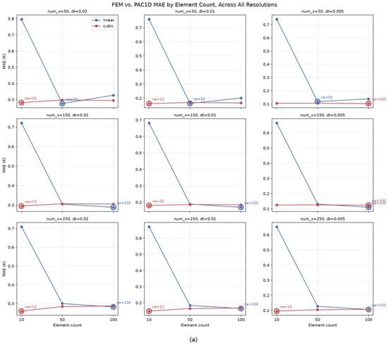
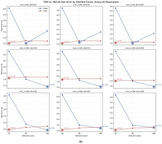
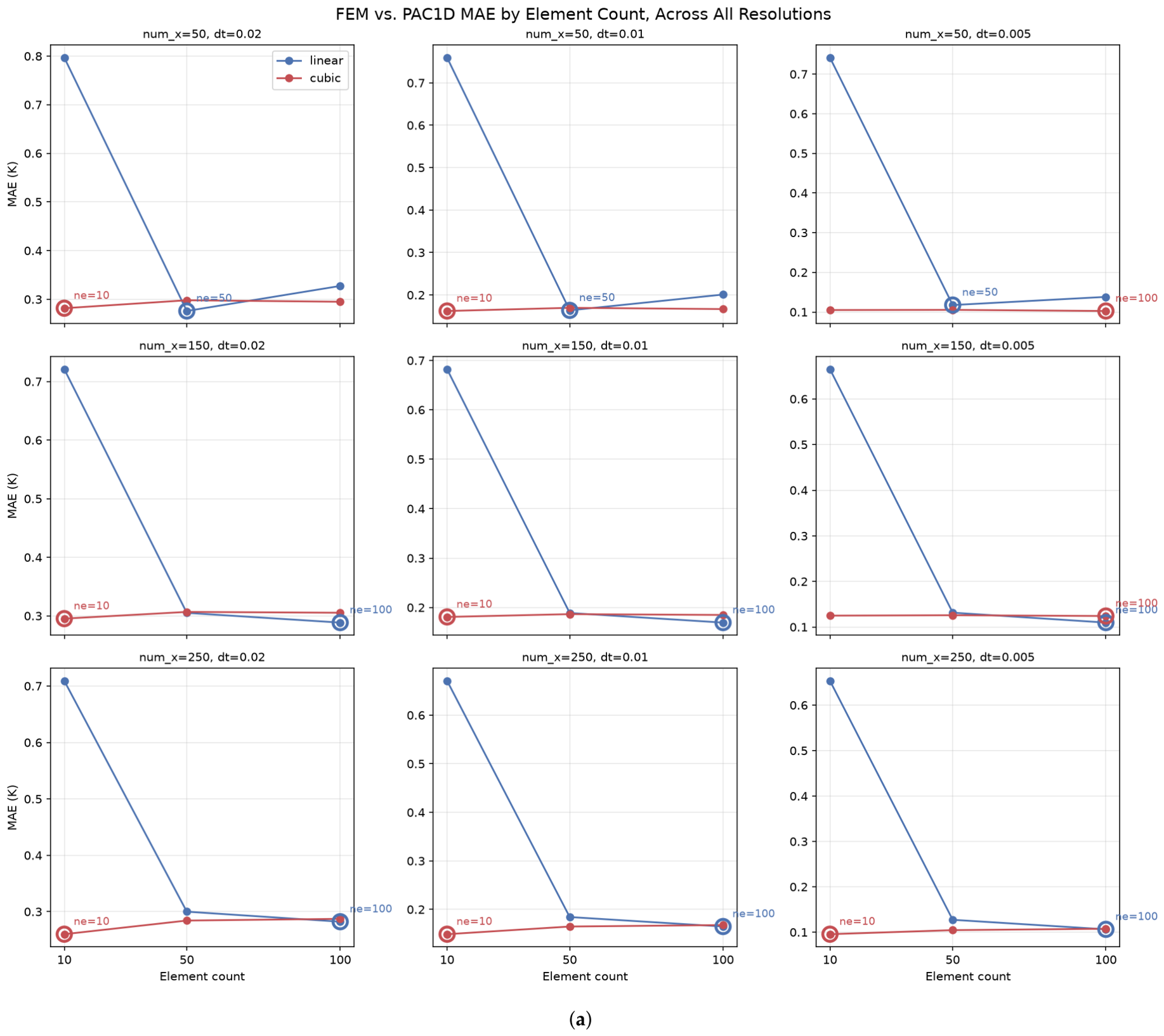
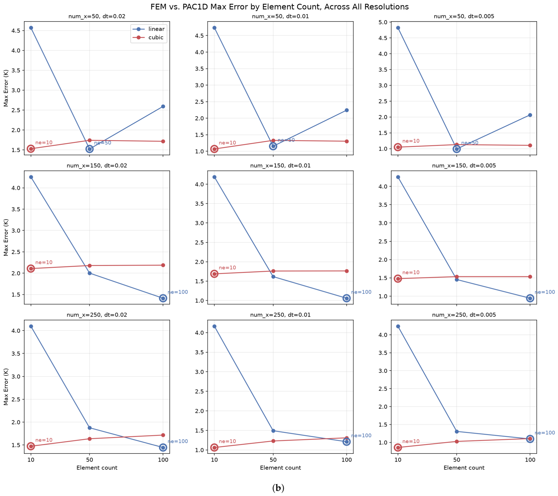
For FEM, two custom implementations are considered: one employing piecewise linear basis functions and another employing piecewise cubic basis functions. Both implementations use Crank–Nicolson time stepping and were run across the same nine spatiotemporal resolutions used for the FDM training data. The element count for each basis was selected empirically: linear and cubic FEM solutions were computed at 10, 50, and 100 elements across all nine resolutions and compared against PAC1D. The cubic basis achieved its lowest error at 10 elements, the smallest count considered, across nearly every resolution and both metrics. For the linear basis, 100 elements achieved a marginally lower mean absolute error than 50 elements in aggregate (0.1986 K versus 0.1993 K, a difference of under 0.4%) and at six of the nine tested resolutions, while 50 elements achieved the lower aggregate maximum error and remained competitive at the coarsest spatial resolution. Given this practically negligible difference in accuracy, 50 elements was selected for the linear basis over 100, offering a reduced computational cost of generating each FEM solution without a meaningful loss in accuracy. These element counts—10 for the cubic basis and 50 for the linear basis—were used for all subsequently reported FEM results.
To validate the custom FEM implementations independently of PAC1D, their solutions were compared against the built-in pdepe solver of MATLAB R2025b (version 25.2), confirming agreement with an established FEM implementation before the custom solvers were used for all subsequent experiments. Because PAC1D also serves as one of the three data-generating solvers compared later in this study, using it as the sole benchmark for FEM accuracy carries an inherent risk of favoring FDM-trained models in that later comparison. We address this directly in Section 3.2 by additionally validating our central findings against a mesh-refinement-verified FEM reference solution.
Finally, to quantify solver agreement beyond visual inspection, two complementary error metrics were computed between each FEM solution and the PAC1D reference: the mean absolute error (MAE) and the maximum absolute error (). MAE provides a physically interpretable measure of the average absolute temperature deviation in Kelvin, while captures the single largest local discrepancy, which is particularly informative given that the largest errors are expected to (and as later shown, do indeed) concentrate near the material interfaces. In general, the closer both metrics are to 0, the better the model is performing. The equations for both metrics are given by
and
where N is the number of sampled points, is the n-th reference temperature, and is the corresponding predicted or numerically solved temperature.
Figure 1 shows the result of the element-count selection process across all nine training resolutions.
Figure 1.
Element-count selection for the piecewise linear and piecewise cubic finite element method (FEM) implementations, evaluated against the Python Ablation Code 1-Dimension (PAC1D) reference across all nine training resolutions (three spatial resolutions × three temporal resolutions per panel). (a) Mean absolute error versus element count. Circled markers indicate the element count achieving the lowest error for each basis. (b) Maximum absolute error versus element count.
As reflected by MAE values ranging from approximately 0.10 to 0.31 K across the nine training resolutions at the selected element counts (Figure 1), the FEM implementations demonstrate close agreement with the PAC1D reference solutions for the triple-layer configuration, particularly at finer discretizations. Despite this generally close agreement, subtle differences in local error distribution and interface behavior may still influence the loss landscape encountered during PINN training.
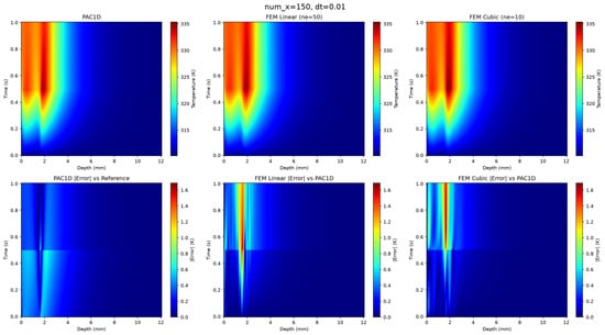
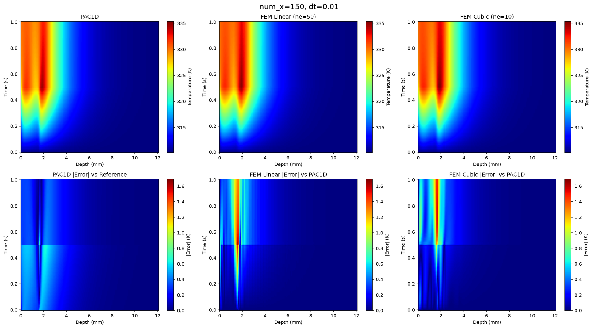
Figure 2 shows representative temperature and error fields for the PAC1D, linear FEM, and cubic FEM solutions at the baseline resolution ( s, ), illustrating the spatial concentration of error near the tissue interfaces described above.
Figure 2.
Predicted temperature fields (top row) and absolute error relative to the PAC1D reference (bottom row) for PAC1D, piecewise linear FEM, and piecewise cubic FEM at the baseline resolution. Error is visibly concentrated at the epidermis–dermis and dermis–fat interfaces for both FEM bases.
2.4. PINN Configuration
2.4.1. Loss Formulation
For all reported PINN experiments, the loss was formulated as a weighted sum of mean squared errors (MSEs), corresponding to the governing physics and available data. Specifically, the loss consists of an initial/boundary condition term, a PDE residual term, and a supervised data term. An expression for the total loss is hence given by
where , , and are weighting coefficients for the initial/boundary condition loss, PDE residual loss, and supervised data loss, respectively. The three MSE terms are defined as
where is the total number of training points for the initial and boundary conditions, is the spatiotemporal coordinate of the n-th training point, is the reference temperature at that point, and is the predicted temperature;
where is the number of collocation points, is the spatiotemporal coordinate of the n-th collocation point, and is the PDE residual evaluated at that point. The PDE residual is given by
where represents the predicted temperature solution, and and are the same as in Equation (4). This residual is obtained by moving all terms to the left-hand side of the equation; and
where is the number of supervised data points, is the spatiotemporal coordinate of the n-th supervised data point, is the reference temperature from a numerical solution at that point, and is the predicted temperature.
2.4.2. Hyperparameter Configuration
Selecting optimal hyperparameters for PINNs remains a challenging and problem-dependent task, though recent works have proposed strategies to improve and generalize the process [18]. In this study, a full factorial ablation was conducted over network depth (1–3 hidden layers), width (8, 16, and 32 neurons per layer), activation function (tanh, rectified linear unit (ReLU), and Gaussian error linear unit (GELU)), and optimization strategy (adaptive moment estimation (Adam), limited-memory Broyden–Fletcher–Goldfarb–Shanno (L-BFGS), and hybrid). All possible combinations were trained on FDM data at the baseline resolution across 20 independent seeds per configuration to assess random seed initialization variability. Table 2 reports MAE and its coefficient of variation (CV) for each depth–width–activation combination, averaged across the three tested optimizer strategies, which were themselves part of the same factorial design and are examined separately in the optimizer-strategy ablation below. CV here serves as a measure of seed-to-seed stability: a low-MAE configuration that is also low-CV is preferable to one that achieves a good mean by chance on some seeds while varying widely on others. We declare 10% as our stability threshold in accordance with the methodologies of similar previous works [19,20]. Twenty seeds per configuration were chosen to provide a computationally tractable estimate of seed-to-seed variability across the scale of the full factorial sweep, balancing statistical reliability against compute budget. Three hidden layers, 32 neurons per layer, and tanh activation jointly achieved the lowest MAE of all 27 combinations. ReLU performed substantially worse than either tanh or GELU at every depth–width combination tested, which we attribute to ReLU’s vanishing second derivative starving the physics-residual loss term of the diffusion information needed to enforce the governing PDE. This architecture (three hidden layers, 32 neurons per layer, tanh activation) was selected and fixed for all subsequently reported experiments.
Table 2.
Mean absolute error (MAE) and seed-to-seed coefficient of variation (CV) for all 27 tested network depth, width, and activation function combinations, averaged across the three tested optimizer strategies: adaptive moment estimation (Adam), limited-memory Broyden–Fletcher–Goldfarb–Shanno (L-BFGS), and hybrid.
A separate ablation was then conducted to select the optimizer strategy. Using the selected architecture, training was repeated under Adam alone, L-BFGS alone, and a hybrid schedule of Adam followed by L-BFGS, across all three solvers and the coarsest, baseline, and finest tested resolutions. Table 3 summarizes the results: Adam alone was both less accurate and less stable than the other two strategies, meeting the 10% CV stability threshold in only 4 of 9 solver-resolution combinations, compared to 8 of 9 for both the hybrid schedule and L-BFGS alone. While hybrid and L-BFGS alone had similar accuracy (≈0.07% difference), L-BFGS alone required roughly half the average training time of the hybrid schedule (20.5 s vs. 39.3 s). L-BFGS alone was therefore selected as the optimizer strategy for all subsequently reported experiments.
Table 3.
Optimizer strategy comparison at the selected architecture (three hidden layers, 32 neurons per layer, tanh activation), averaged across nine solver-resolution combinations (three solvers × coarsest, baseline, and finest tested resolutions).
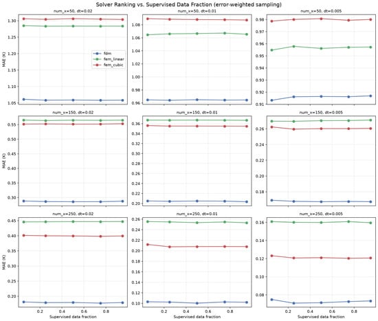
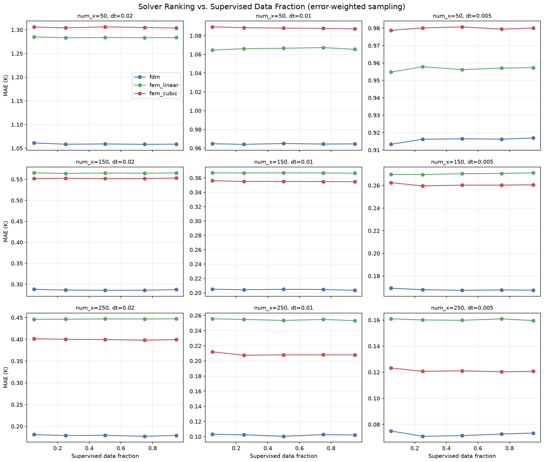
The number of supervised data points was determined separately. Five supervised-data fractions (5%, 25%, 50%, 75%, and 95% of the number of collocation points) were tested across every solver and resolution (using error-weighted sampling described in the paragraph below), and the resulting solver-choice ranking was found to be identical at every tested fraction (Figure 3), indicating no meaningful interaction between data quantity and solver choice; hence, 25% was safely retained as a representative default for all subsequently reported results. The number of collocation, boundary, and initial condition points (5000, 250, and 250, respectively) is consistent with, and more conservative than, the ratios used in the original PINN formulation [6], which used collocation-to-boundary/initial-condition ratios of 100:1 and 200:1 for its Burgers’ and Schrödinger equation benchmarks, respectively, compared to the 20:1 ratio used here. The substantially larger collocation count relative to the boundary and initial condition counts reflects that collocation points must resolve the governing PDE over the full two-dimensional spatiotemporal domain, whereas boundary and initial condition points constrain only one-dimensional slices of that domain. These counts were fixed across all reported experiments, and thus the final hyperparameter configuration used in all reported experiments is summarized in Table 4.
Figure 3.
Mean absolute error versus supervised data fraction for each of the three solvers, faceted by resolution (error-weighted sampling).
Table 4.
PINN hyperparameters used for all reported experiments.
Although coupled into the same loss term, boundary and initial condition points were sampled independently. Boundary and interior collocation points were sampled uniformly across their respective domains, and all initial condition points were obtained directly from the reference solution. Two strategies for sampling supervised data points were compared: uniform sampling across the spatiotemporal domain, and error-weighted sampling, which biases point selection toward regions of largest disagreement among the three numerical solvers (predominantly the material interfaces). The latter was found to substantially improve training stability, particularly at fine resolutions, and is discussed further in Section 3.3. Rather than fixed, unit loss weights, an adaptive weighting scheme following [14] was used for all reported experiments, recomputed per training run from the training data itself.
where is the number of loss terms and is the mean squared magnitude of loss term i’s target values. Lastly, Z-score standardization was applied to temperature data and forcing values for training, and unscaled for predictions.
2.4.3. Evaluation
As with the numerical methods, PINN performance was also evaluated using MAE and . For each numerical method and training resolution, MAE and were averaged over 20 independent seeds to account for potential variability caused by random seed initialization, and stability was assessed using the same 10% threshold CV introduced in Section 2.4.2 above. Across the final set of reported experiments, CV ranged from approximately 0.4% to 7.5%, with all 27 tested solver-resolution combinations meeting this threshold. Average training time was also reported for each case, similarly averaged over the 20 seeds, though this is of secondary importance given that a PINN, once trained, does not require retraining for inference. As a complementary, accuracy-independent measure of training efficiency, we additionally computed the number of L-BFGS iterations required for each run’s total loss to first fall below a fixed threshold, at the baseline resolution. FEM-trained models reached this threshold in fewer iterations on average than FDM-trained models (approximately 289 for both FEM bases combined, versus 327 for FDM), despite FDM-trained models ultimately achieving lower final error: FDM’s accuracy advantage is not explained by, nor does it translate into, faster convergence during training.
3. Results
This section presents three sets of findings: the central comparison of PINN accuracy across training-data solver and resolution, an independent validation of this comparison against an FEM reference, and the effect of supervised-data sampling strategy on training stability.
3.1. PINN Accuracy Across Solvers and Resolutions
Table 5 reports MAE, Max Error, and the seed-to-seed CV for each of the three solvers at each of the nine tested resolutions, using the architecture, optimizer strategy, and supervised-data fraction established in Section 2.4.2, with error-weighted supervised-data sampling. FDM-trained models achieved the lowest MAE at every one of the nine tested resolutions. Among the two FEM bases, the linear basis outperforms the cubic basis only at the coarsest spatial resolution (). At all finer spatial resolutions, the cubic basis outperforms the linear basis, independent of temporal resolution. All 27 tested configurations met the 10% CV stability threshold, though CV was consistently highest for FDM-trained models at the finest tested spatial resolution (), across all three temporal resolutions.
Table 5.
PINN performance by solver and training resolution, using error-weighted supervised-data sampling at 25% data fraction.
Because prediction error is expected to concentrate near the tissue-layer interfaces, Table 6 additionally reports MAE and Max Error within a 0.5 mm neighborhood of each interface, for the same 27 solver-resolution configurations. Interface-region MAE is consistently higher than the corresponding domain-averaged MAE from Table 5, by a factor of roughly two to four across the tested configurations, confirming that global metrics alone understate the error incurred near material discontinuities.
Table 6.
Interface-windowed MAE and Max Error by solver and training resolution, within 0.5 mm of the epidermis-dermis and dermis-fat interfaces, using the same configurations as Table 5.
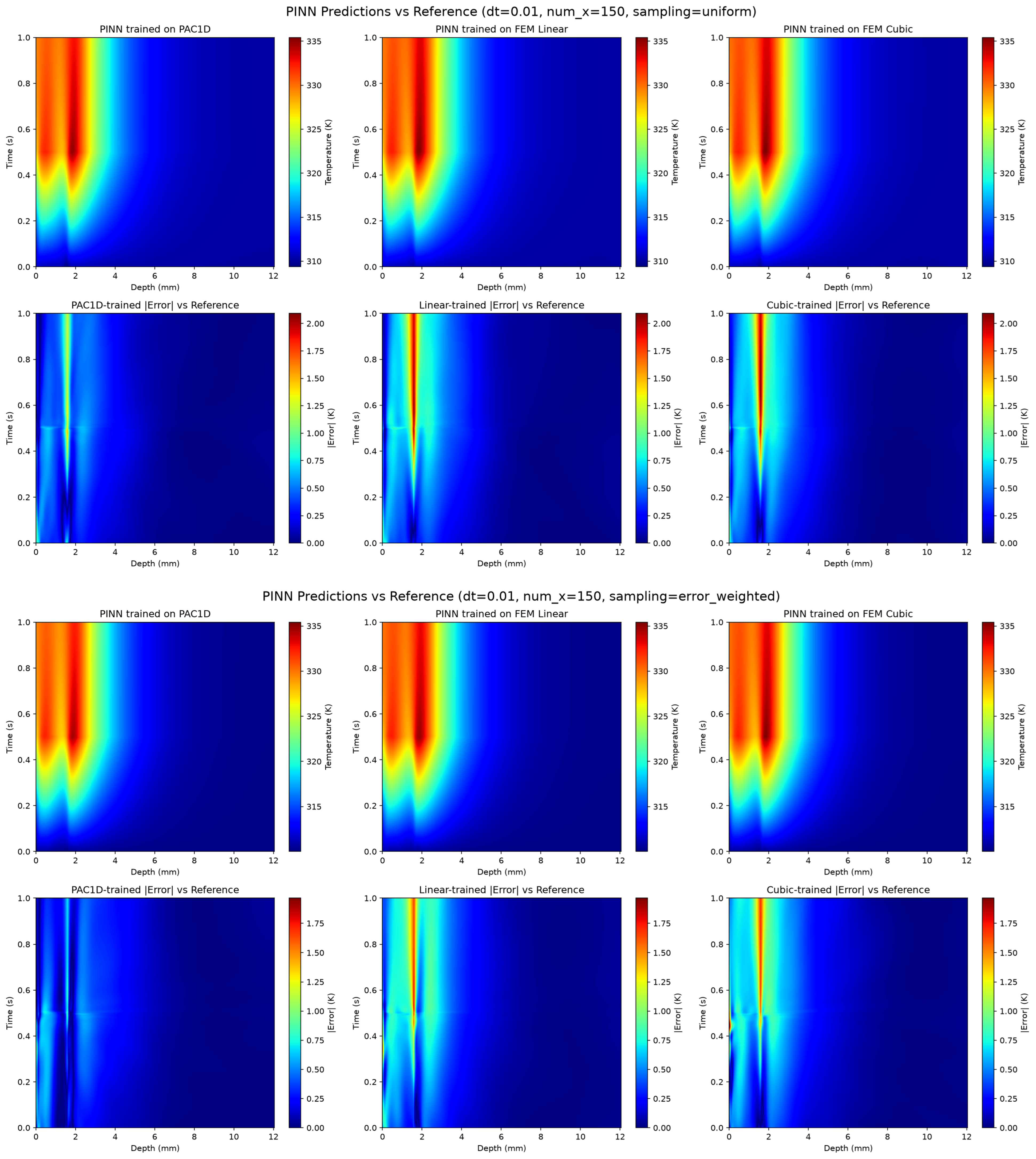
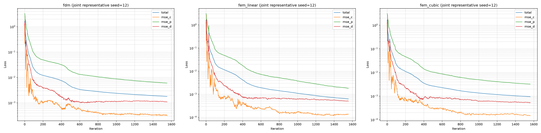
Figure 4 shows full-field predictions and absolute error relative to the reference solution for each solver at the baseline resolution, under both uniform and error-weighted supervised-data sampling, using one seed shared across all three solvers so that the comparison is not confounded by differences in random network initialization between solvers. Consistent with the numerical solver comparison of Section 2.3, prediction error concentrates near the tissue-layer interfaces for all three solvers, with the FDM-trained model exhibiting visibly lower error than either FEM-trained model across most of the domain. Figure 5 shows the complete training loss histories for that same shared seed at the baseline resolution.
Figure 4.
Representative full-field PINN predictions and absolute error relative to the reference solution at the baseline resolution, for each solver, under uniform (top) and error-weighted (bottom) supervised-data sampling.
Figure 5.
Training loss history at the baseline resolution for a representative seed of each solver (FDM, piecewise linear FEM, piecewise cubic FEM), showing total loss and its three components (mse_c: boundary/initial condition; mse_p: PDE residual; mse_d: supervised data) on a log scale. Since all reported experiments used L-BFGS alone (Section 2.4.2), no Adam phase is shown.
3.2. Validation Against an FEM Reference
As mentioned in Section 2.3, because the reference solution used throughout this study is itself generated by PAC1D—the same solver family as one of the three training-data sources compared above—we validated the central solver comparison against a mesh-refinement-verified FEM reference. To verify this reference itself, we performed a mesh-refinement convergence study, solving the piecewise linear FEM formulation at 50, 100, 150, and 200 elements on the same fine spatiotemporal grid as our reference solution: across the full domain, the 150- and 200-element solutions agree to within 0.036 K on average, tightening to 0.0035 K when a 0.5 mm neighborhood of each material interface is excluded. Within that neighborhood, a localized region of residual mesh sensitivity remains, most pronounced at the dermis-fat boundary (0.17 K on average, 0.59 K maximum, between the 150- and 200-element solutions). We report this honestly as a limitation applicable to any numerical reference in this class of problem, including our own, and used the 200-element solution as our independent FEM reference below. Table 7 compares the resulting solver ranking under both references at each of the nine tested resolutions. The ranking is identical under both references at 8 of the 9 resolutions. The finest tested resolution ( s, ) sees cubic basis FEM narrowly outperforming FDM under the FEM reference (0.0866 K versus 0.0885 K), a difference smaller than the reference’s own residual interface uncertainty noted above and therefore not distinguishable from it. We interpret this as evidence that FDM-trained models achieving the lowest error is not an artifact of evaluating against a solver-matched reference, while noting that the reference’s own interface-region uncertainty is the most likely explanation for this single exception, and that comparably sized solver differences at other resolutions should be interpreted with this same caveat in mind.
Table 7.
Solver ranking (best to worst, by mean absolute error) at each of the nine training resolutions, under the original PAC1D-family reference and the FEM reference (5 seeds per configuration).
3.3. Effect of Supervised-Data Sampling Strategy
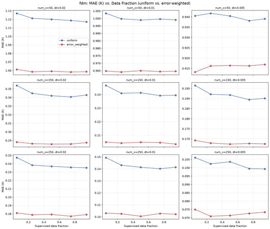
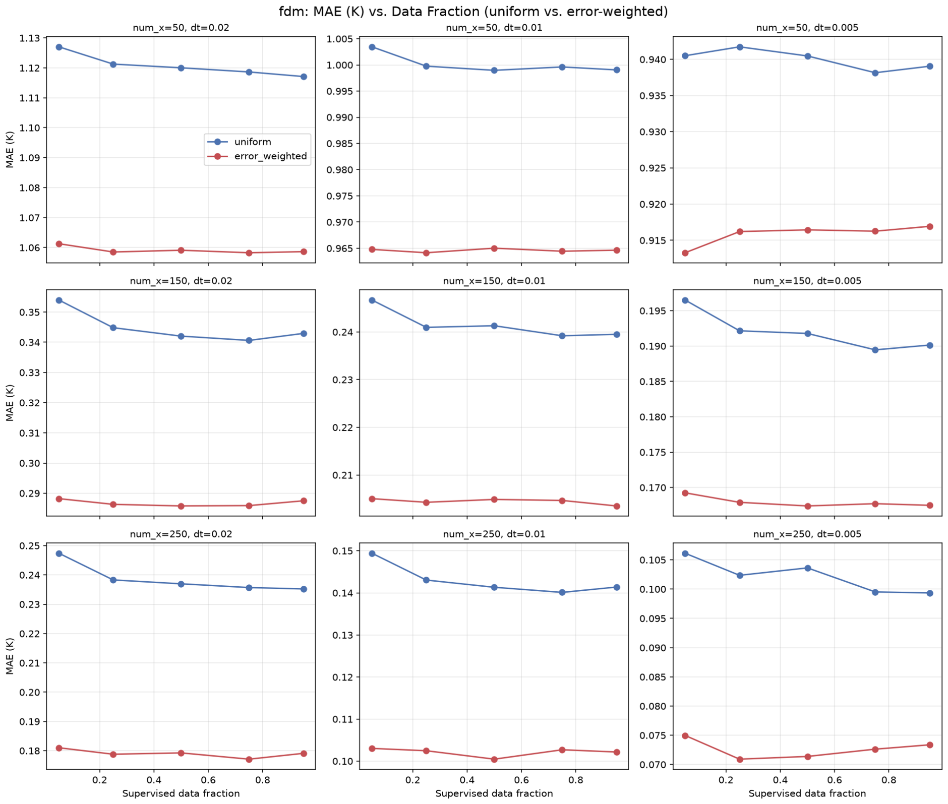
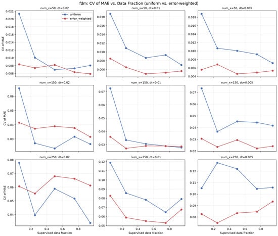
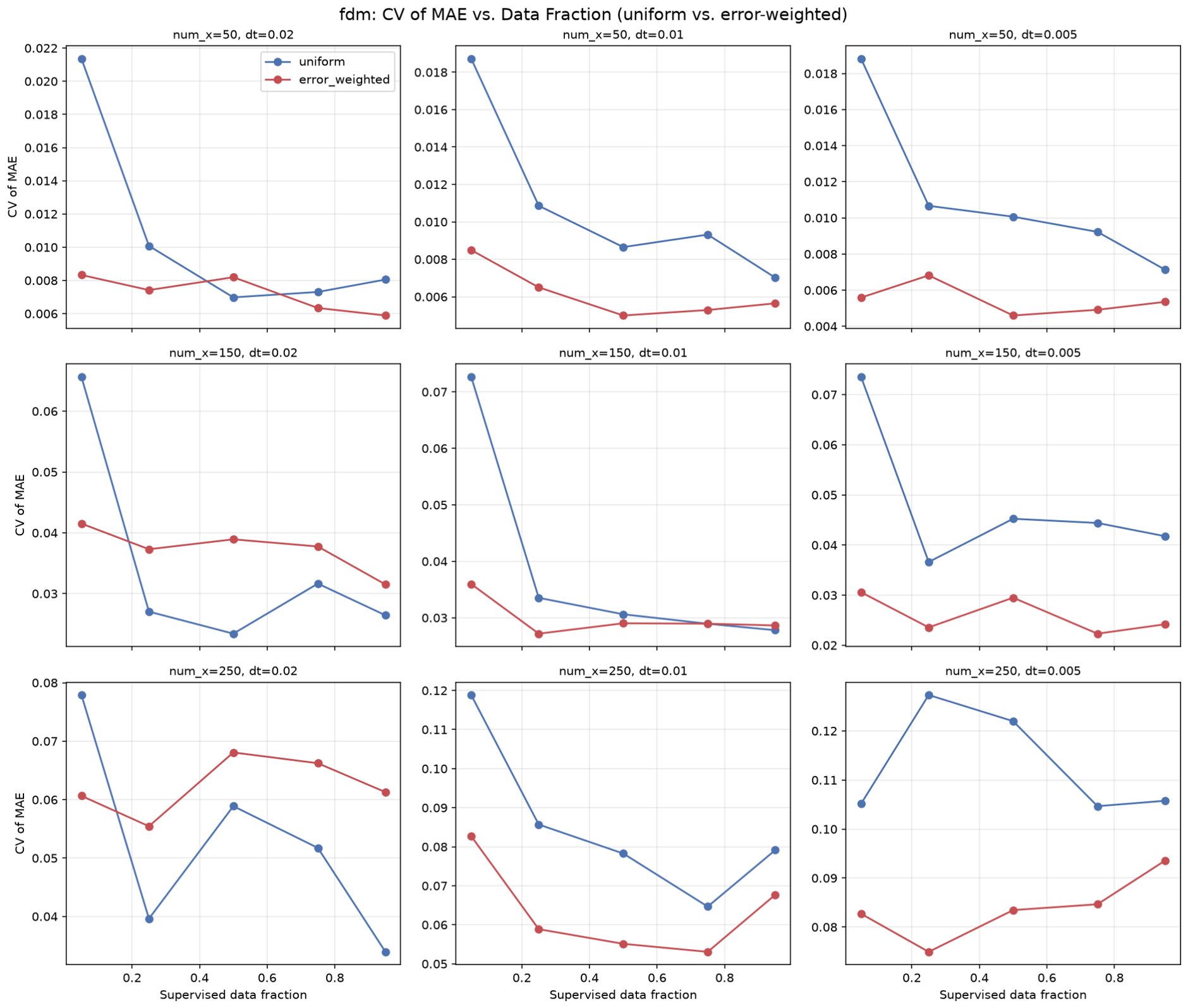
Figure 6 and Figure 7 show mean absolute error and CV, respectively, as a function of supervised-data fraction for FDM-trained models, comparing uniform and error-weighted sampling across all nine training resolutions. The corresponding results for the piecewise linear and piecewise cubic FEM solvers are given in Appendix A. Error-weighted sampling consistently reduced CV relative to uniform sampling, with the effect most pronounced at finer resolutions. The largest single improvement occurred for FDM at the finest tested resolution and 25% data fraction, where CV fell from 12.7% under uniform sampling to 7.5% under error-weighted sampling. This effect is independent of the solver-choice comparison reported above: for every solver and resolution tested, error-weighted sampling did not change which solver achieved the lowest error, but did improve the consistency with which that error was achieved across random seed initialization.
Figure 6.
Mean absolute error versus supervised data fraction for FDM-trained models, faceted by resolution, comparing uniform and error-weighted supervised-data sampling.
Figure 7.
Seed-to-seed coefficient of variation versus supervised data fraction for FDM-trained models, faceted by resolution, comparing uniform and error-weighted supervised-data sampling.
4. Discussion
Across the nine tested spatiotemporal resolutions, PINNs supplemented with FDM-generated data achieved the lowest prediction error at every resolution, with the advantage over both FEM bases robust to validation against the FEM reference. This advantage narrowed as spatiotemporal resolution increased, becoming indistinguishable from the cubic FEM basis only at the single finest resolution tested. We interpret this pattern as evidence that the numerical characteristics of supervisory training data do have an effect on PINN training, though this effect diminishes as the underlying numerical solvers themselves converge toward closer mutual agreement at finer discretization. This interpretation is further supported by each solver’s pre-training disagreement with the reference solution and its corresponding trained PINN’s final accuracy: solvers that agreed more closely with the reference before training also produced more accurate PINNs after training, suggesting that solver-induced error propagates through training.
A second, independent finding is that biasing supervised-data sampling toward regions of known disagreement among the numerical solvers (in this case the tissue-layer interfaces) meaningfully improves training stability across random seed initialization, particularly at fine resolution, without changing which solver produces the most accurate model. Practitioners can therefore obtain more consistent PINN training outcomes by concentrating supervision where the underlying data is least certain, rather than sampling uniformly across the domain, independent of which numerical solver is used to generate training data.
Importantly, it should be noted that this study considers the one-dimensional heat equation with fully known governing physics and a single, anatomically representative three-layer skin configuration. The network architecture, optimizer strategy, and supervised-data fraction used throughout were each fixed based on dedicated ablations and confirmed not to materially affect the reported solver comparison. The insulated (homogeneous Neumann) boundary conditions are also a simplification relative to physiological heat exchange at the skin surface. This is a reasonable choice for a controlled numerical study but should be borne in mind when extending these findings toward more biologically representative laser–skin interactions. We have not tested higher-dimensional domains, sharper solution gradients, additional material discontinuities, or complex spatiotemporal source terms, any of which may alter the extent to which solver-induced differences propagate through hybrid PINN training. The present findings establish that solver choice matters in a precise and resolution-dependent way for this class of problem, rather than establishing general solver properties, and future work should extend this comparison to higher-dimensional and partially known physical systems to determine whether the same resolution-dependent pattern holds more broadly.
5. Conclusions
PINNs trained on FDM-generated data achieved the lowest prediction error among the three solvers tested at every one of nine spatiotemporal resolutions spanning coarse to fine discretization, an advantage confirmed robust to validation against the FEM reference, with the solver ranking matching under both references at 8 of the 9 resolutions and narrowing to an indistinguishable difference between FDM and cubic FEM at the single finest resolution tested. These results indicate that, under the controlled physical conditions and fixed network architecture considered in this study, the choice of numerical solver used to generate supervisory training data does influence hybrid PINN predictive accuracy in a measurable and quantifiable way, with the practical size of this effect diminishing as training-data resolution increases. For practitioners, these results highlight the value of evaluating the numerical scheme and associated discretization settings for the physics and geometry of interest, as FDM-generated training data yielded lower error at coarse-to-moderate resolutions, while the choice between FDM and cubic FEM becomes practically inconsequential at sufficiently fine discretization. Independent of this solver comparison, biasing supervised-data sampling toward regions of known inter-solver disagreement was found to meaningfully improve training stability across random seed initialization, particularly at fine resolution. These findings are scoped to the one-dimensional, fully-specified diffusion setting considered here, and extending this comparison to higher-dimensional or partially known physical systems remains an open direction for future work.
Author Contributions
Conceptualization, S.W. and T.K.; methodology, H.Y. and S.W.; software, H.Y., S.W., C.P. and J.Q.; validation, H.Y.; formal analysis, T.K.; investigation, H.Y. and J.Q.; resources, T.K.; data curation, H.Y.; writing—original draft preparation, H.Y.; writing—review and editing, C.A.O. and T.K.; visualization, H.Y.; supervision, T.K.; project administration, T.K.; funding acquisition, T.K. All authors have read and agreed to the published version of the manuscript.
Funding
This research was supported by the Air Force Research Laboratory under Award No. FA8650-20-2-5853.
Institutional Review Board Statement
Not applicable.
Informed Consent Statement
Not applicable.
Data Availability Statement
The code and data supporting the findings of this study will be made available upon request.
Acknowledgments
This project was supported in part by an appointment to the National Research Council (NRC) Research Associateship Program at the 711th Human Performance Wing’s Tri-Service Research Laboratory, administered by the Fellowships Office of the National Academies of Sciences, Engineering, and Medicine. Support from the Air Force Research Laboratory’s Science and Technology Fellowship Program is gratefully acknowledged.
Conflicts of Interest
The authors declare no conflicts of interest.
Appendix A. Supplementary Sampling-Strategy Results
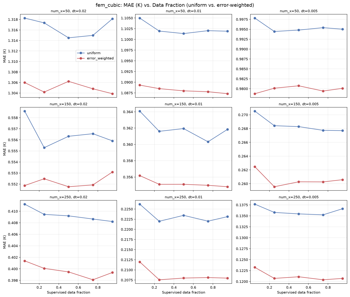
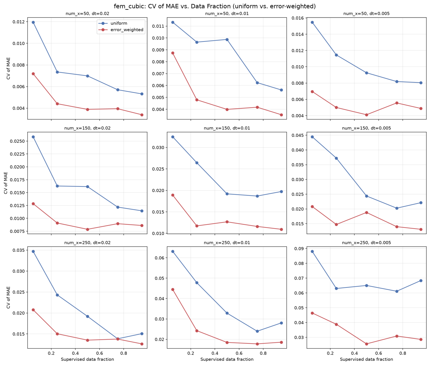
Figure A1 and Figure A2 show mean absolute error and CV versus supervised data fraction for the piecewise linear and piecewise cubic FEM solvers, respectively, complementing the FDM results shown in Figure 6 and Figure 7.
Figure A1.
(top) Mean absolute error versus supervised data fraction for piecewise linear FEM-trained models, faceted by resolution, comparing uniform and error-weighted supervised-data sampling. (bottom) CV versus supervised data fraction for piecewise linear FEM-trained models, faceted by resolution, comparing uniform and error-weighted supervised-data sampling.
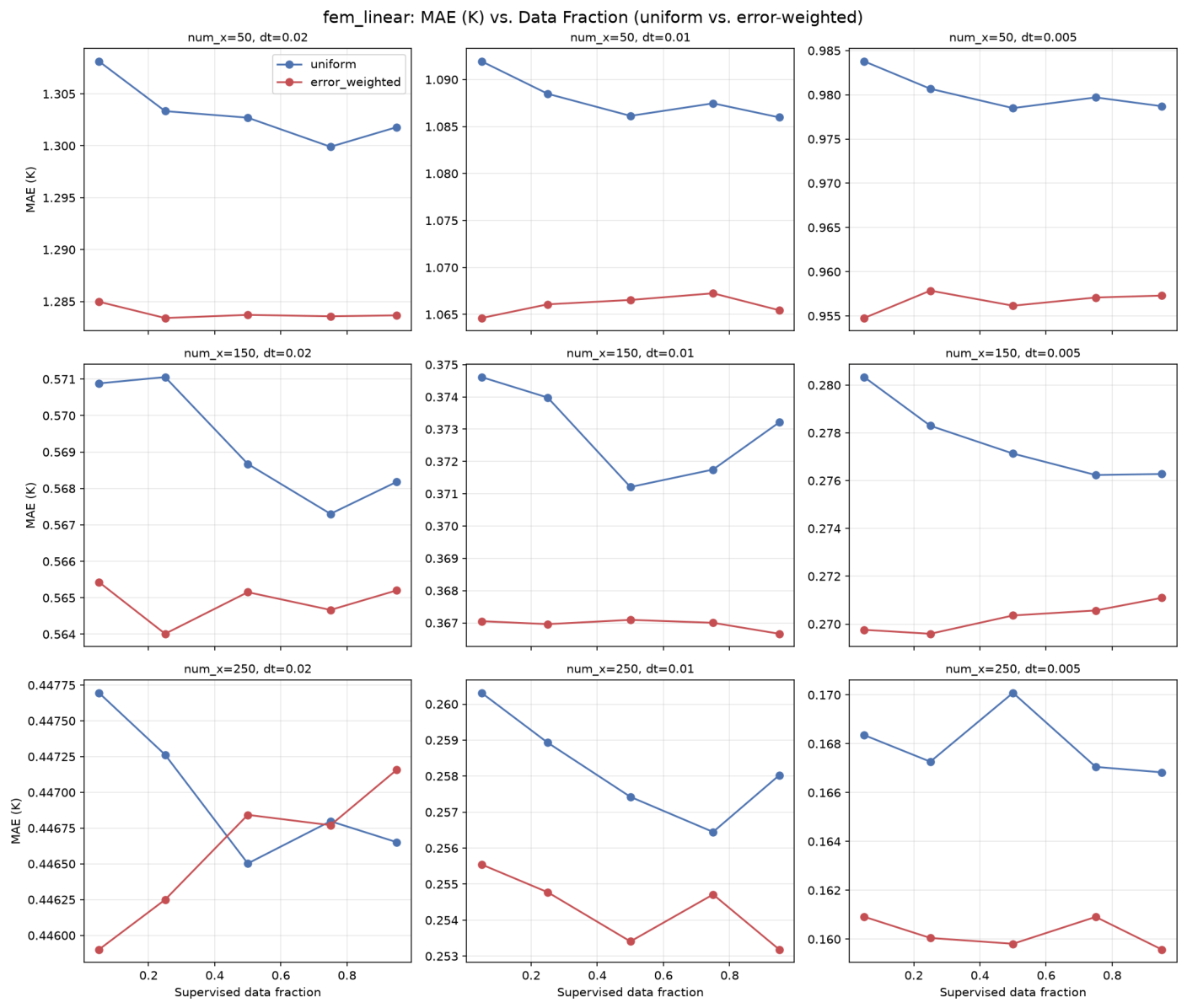
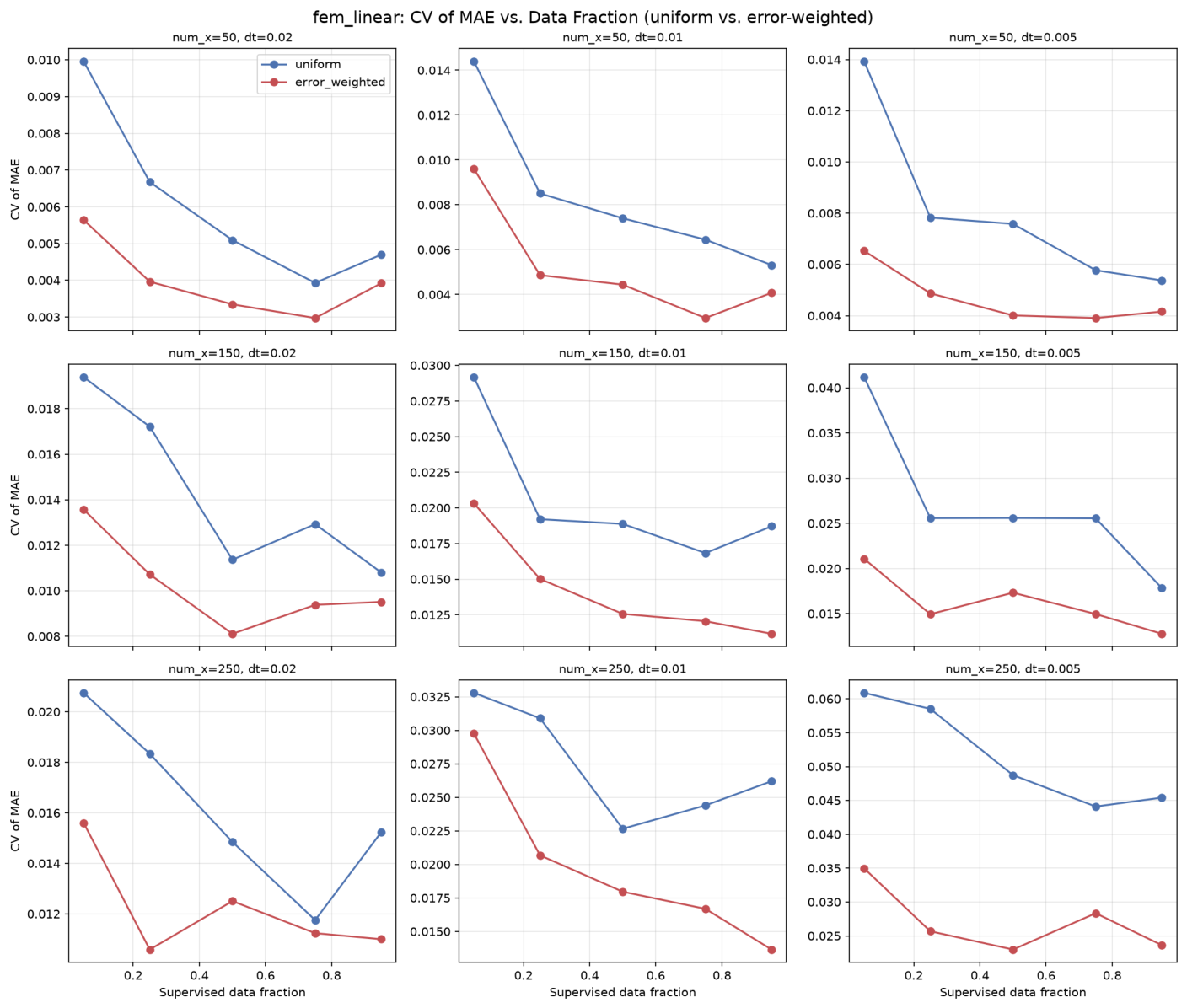
Figure A2.
(top) Mean absolute error versus supervised data fraction for piecewise cubic FEM-trained models, faceted by resolution, comparing uniform and error-weighted supervised-data sampling. (bottom) CV versus supervised data fraction for piecewise cubic FEM-trained models, faceted by resolution, comparing uniform and error-weighted supervised-data sampling.
References
- Wongchadakul, P.; Rattanadecho, P.; Jiamjiroch, K. Experimental analysis of thermal transport in low-level laser therapy on skin tissue: The influence on therapeutic efficacy, pain sensation and dry skin wound. Int. J. Therm. Sci. 2024, 199, 108886. [Google Scholar] [CrossRef] [Scilit]
- Alshanti, W.G.; Batiha, I.M.; Abu Hammad, M.; Khalil, R. A novel analytical approach for solving partial differential equations via a tensor product theory of Banach spaces. Partial Differ. Equ. Appl. Math. 2023, 8, 100531. [Google Scholar] [CrossRef] [Scilit]
- Toledo-Marín, J.Q.; Fox, G.; Sluka, J.P.; Glazier, J.A. Deep learning approaches to surrogates for solving the diffusion equation for mechanistic real-world simulations. Front. Physiol. 2021, 12, 667828. [Google Scholar] [CrossRef] [Scilit] [PubMed]
- Chen, R.; Wu, K. A comparison study of deep Galerkin method and deep Ritz method for elliptic problems with different boundary conditions. Commun. Math. Res. 2020, 36, 354–376. [Google Scholar] [CrossRef] [Scilit]
- Zhou, A.; Barati Farimani, A. Predicting change, not states: An alternate framework for neural PDE surrogates. Comput. Methods Appl. Mech. Eng. 2025, 441, 117990. [Google Scholar] [CrossRef] [Scilit]
- Raissi, M.; Perdikaris, P.; Karniadakis, G.E. Physics-informed neural networks: A deep learning framework for solving forward and inverse problems involving nonlinear partial differential equations. J. Comput. Phys. 2019, 378, 686–707. [Google Scholar] [CrossRef] [Scilit]
- Krishnapriyan, A.S.; Gholami, A.; Zhe, S.; Kirby, R.M.; Mahoney, M.W. Characterizing possible failure modes in physics-informed neural networks. arXiv 2021, arXiv:2109.01050. [Google Scholar]
- Velioglu, M.; Zhai, S.; Rupprecht, S.; Mitsos, A.; Jupke, A.; Dahmen, M. Physics-informed neural networks for dynamic process operations with limited physical knowledge and data. Comput. Chem. Eng. 2025, 192, 108899. [Google Scholar] [CrossRef] [Scilit]
- Liu, Y.; Liao, S.; Yang, Y.; Zhang, B. Data-driven and physics-informed neural network for predicting tunnelling-induced ground deformation with sparse data of field measurement. Tunn. Undergr. Space Technol. 2024, 152, 105951. [Google Scholar] [CrossRef] [Scilit]
- Mazumder, S. The finite difference method. In Numerical Methods for Partial Differential Equations; Academic Press: Cambridge, MA, USA, 2016; pp. 51–101. [Google Scholar]
- Jagota, V.; Sethi, A.; Kumar, K. Finite element method: An overview. Walailak J. Sci. Technol. 2013, 10, 1–8. [Google Scholar] [CrossRef] [Scilit]
- Florin, J. Comparative analysis of finite difference and finite element method for audio waveform simulation. arXiv 2025, arXiv:2507.05396. [Google Scholar]
- Ajithkumar Sophiya, A.; Nair, A.K.; Maleki, S.; Krishnababu, S.K. A comprehensive analysis of PINNs: Variants, applications, and challenges. arXiv 2025, arXiv:2505.22761. [Google Scholar]
- Farmer, J.; Oian, C.A.; Bowman, B.A.; Khan, T. Empirical loss weight optimization for PINN modeling laser bio-effects on human skin for the 1D heat equation. Mach. Learn. Appl. 2024, 16, 100563. [Google Scholar] [CrossRef] [Scilit]
- Bowman, B.; Oian, C.; Kurz, J.; Khan, T.; Gil, E.; Gamez, N. Physics-informed neural networks for the heat equation with source term under various boundary conditions. Algorithms 2023, 16, 428. [Google Scholar] [CrossRef] [Scilit]
- He, R.; Chen, Y.; Yang, Z.; Huang, J.; Guan, X. Phase field smoothing-PINN: A neural network solver for partial differential equations with discontinuous coefficients. Comput. Math. Appl. 2024, 171, 188–203. [Google Scholar] [CrossRef] [Scilit]
- Arata, J.; Dodd, C.; Lee, T.; Liska, S.; Zollars, B.G.; Thomas, R.J. Python Ablation Code—One Dimension (PAC1D) v3.5; Technical Report; Air Force Research Laboratory, 711th Human Performance Wing, Airman Systems Directorate, Bioeffects Division, Optical Radiation Bioeffects Branch: San Antonio, TX, USA, 2019. [Google Scholar]
- Escapil-Inchauspé, P.; Ruz, G.A. Hyper-parameter tuning of physics-informed neural networks: Application to Helmholtz problems. Neurocomputing 2023, 561, 126826. [Google Scholar] [CrossRef] [Scilit]
- Coleman, C.; Kang, D.; Narayanan, D.; Nardi, L.; Zhao, T.; Zhang, J.; Bailis, P.; Olukotun, K.; Re, C.; Zaharia, M. Analysis of DAWNBench, a Time-to-Accuracy Machine Learning Performance Benchmark. arXiv 2019, arXiv:1806.01427. [Google Scholar]
- Phoon, K.K.; Kulhawy, F.H. Characterization of geotechnical variability. Can. Geotech. J. 1999, 36, 612–624. [Google Scholar] [CrossRef] [Scilit]

Disclaimer/Publisher’s Note: The statements, opinions and data contained in all publications are solely those of the individual author(s) and contributor(s) and not of MDPI and/or the editor(s). MDPI and/or the editor(s) disclaim responsibility for any injury to people or property resulting from any ideas, methods, instructions or products referred to in the content. |
© 2026 by the authors. Licensee MDPI, Basel, Switzerland. This article is an open access article distributed under the terms and conditions of the Creative Commons Attribution (CC BY) license.