Fuel-Efficient Multi-Sortie Scheduling for Forestry Helicopter Spraying Using Hybrid Adaptive Large Neighborhood Search with Sortie Consolidation

Abstract

Forestry helicopter spraying requires fuel-efficient allocation of coverage tasks to successive sorties. Coverage-path generation alone does not resolve this allocation under coupled pesticide depletion and load-dependent fuel consumption. We formulate a Multi-Sortie Routing Problem with Non-synchronous Dual Resources (MSRP-NDR) and develop Sortie-Consolidation Hybrid Adaptive Large Neighborhood Search (SC-HALNS) to minimize modeled fuel consumption under pesticide-capacity and fuel constraints. For fixed coverage paths generated by convex decomposition and the Vector Modeling Method, the framework combines adaptive destroy-and-repair search and randomized variable neighborhood descent, supplemented by whole-sortie consolidation. Only merges that preserve resource feasibility and reduce total modeled fuel consumption are accepted. Six GIS-derived forest instances with 10–102 tasks were evaluated using 20 runs per stochastic algorithm and a nominal 100 s search budget. Relative to the aviation-company practice method (ACPM), SC-HALNS reduced mean modeled fuel consumption by 1.31–7.87%. Exact paired sign tests with Holm correction favored SC-HALNS in 13 of 18 external comparisons. Accepted consolidations reduced returns to the base, potentially easing replenishment workload. These results support offline scheduling under the evaluated model assumptions; reported fuel savings are model-based estimates.

1. Introduction

Aerial plant protection is widely used for agricultural and forestry pest and disease control [1,2]. Forestry spraying operations often involve extensive treatment areas, irregular boundaries, and spatially scattered plots. Manned helicopters can serve large forest areas, but their operating costs make route and sortie planning important for operational efficiency [3]. A scheduling method must therefore coordinate coverage tasks, transfer flights, and replenishment while accounting for pesticide availability and fuel consumption.

Coverage path planning determines how an aircraft traverses a target area while providing the required coverage [4,5]. Geometric decomposition and systematic sweeping patterns are commonly used to construct coverage paths [6,7,8]. For irregular boundaries, the choice of decomposition and scanning direction affects route length, turning requirements, and non-spraying travel [7,9,10].

For helicopter spraying, Fang et al. [11] combined the Vector Modeling Method (VMM) with a double-layer nested improved genetic algorithm (DNiGA). VMM evaluates turns and extra coverage, while DNiGA optimizes inter-region visiting order and entry/exit choices using dispatch distance. Their field experiment also reported reduced fuel consumption. The reported field savings supported the route-planning approach under study, whose dispatch objective was distance rather than modeled complete-sortie fuel consumption. Fang et al. [12] subsequently combined spraying-route generation and dispatch routing with temporary takeoff and landing site (TTSL) selection, restricting candidate sites to suitable areas. Related work further examined site-location optimization [13]. These studies show how coverage geometry, regional sequencing, and site selection influence helicopter operations. However, a shorter dispatch route alone does not establish the best allocation of spraying tasks to resource-feasible sorties when the fuel cost changes with aircraft mass. Here, we retain VMM-based coverage generation but optimize task-to-sortie assignments and visiting orders using complete-sortie fuel evaluation. Our fixed coverage paths and fixed TTSL narrow the decision scope relative to the site-and-route planning in [12]; the present study does not replace those planning decisions.

Energy and replenishment have also been incorporated into agricultural UAV coverage planning. Yu et al. [14] optimized the heading of three-dimensional coverage paths, using an energy model that accounts for terrain, changing pesticide load, and replenishment flights. Their study assumes battery replacement during liquid replenishment. Lara-Molina [15] combined weed detection with coverage-path and visiting-order optimization, minimizing mission time while allowing returns to the depot under a flight-endurance limit. These approaches establish that energy-aware spraying and replenishment are existing research directions. The present formulation instead evaluates helicopter fuel consumption while tracking pesticide depletion during spraying and fuel depletion throughout each sortie. It addresses the grouping and sequencing of fixed coverage tasks under this coupled resource model; it does not optimize three-dimensional coverage geometry or weed detection. The studies therefore differ in their decision variables, resource representations, and objectives, and their reported improvements should not be treated as directly comparable performance measures.

In the wider routing literature, the Multi-Trip Vehicle Routing Problem (MTVRP) allows vehicles to perform several depot-based routes within a planning horizon [16,17]. For example, the MTVRP formulation of Cattaruzza et al. [17] minimizes total travel time subject to vehicle-capacity and working-day constraints. The present problem shares the repeated-departure and replenishment structure of these models. Fuel-aware routing is also established: the Pollution–Routing Problem accounts for load- and speed-dependent fuel costs [18], and its ALNS solution approach includes speed optimization [19]. Repeated trips and load-dependent fuel consumption are therefore established concepts on which this study builds.

The specific modeling issue here is their combination with the execution of fixed helicopter spraying paths. Each coverage task comprises an entry point, an exit point, and an internal flight path, rather than only a customer location. Pesticide is discharged only along spraying segments, whereas fuel is consumed during spraying, transfers, turning connections, and travel to and from the TTSL. Both remaining pesticide and remaining fuel contribute to aircraft mass and hence to subsequent fuel consumption. Under the prescribed flight speed, task allocation and visiting order must therefore be evaluated using the evolving resource states over each complete sortie, including its return flight. The resulting MSRP-NDR is an application-specific multi-trip routing formulation with coupled resource consumption. Its focus is to organize fixed coverage tasks into feasible sorties with low modeled fuel consumption; the internal coverage paths and TTSL location are fixed before scheduling.

Adaptive large neighborhood search (ALNS) provides a flexible framework for constrained routing problems. It modifies solutions through task removal and reinsertion, with operator selection adapted according to previous search performance [20,21]. This structure allows task assignments and visiting orders to be revised within the same search process. Reviews of ALNS document a wide range of hybrid designs and removal and insertion operators for routing applications [22,23]. Randomized variable neighborhood descent (RVND) provides an approach complementary to local improvement by exploring multiple neighborhoods in a randomized order [24]. These search principles offer a basis for helicopter sortie scheduling, provided that candidate changes are evaluated using the pesticide requirements and fuel consumption of the complete affected sorties.

Some schedules contain sorties with small spraying workloads, each requiring travel to and from the TTSL. Consolidating their tasks can reduce return and replenishment frequency and the associated ground support effort. Whole-sortie consolidation is therefore introduced as a supplementary function to HALNS, with pesticide and fuel feasibility and the resulting change in modeled fuel consumption determining whether a merge is accepted.

To address this scheduling problem, we develop SC-HALNS for fixed coverage tasks generated by convex decomposition and VMM. The main contributions are as follows:

(1)

Problem formulation and fuel evaluation. We formulate forestry helicopter spraying as a Multi-Sortie Routing Problem with Non-synchronous Dual Resources (MSRP-NDR). Task-to-sortie assignments and visiting orders are evaluated under pesticide-capacity and fuel constraints, accounting for pesticide use during spraying and load-dependent fuel consumption throughout each complete sortie, including its return flight.

(2)

Whole-sortie consolidation within HALNS. We supplement HALNS, which combines adaptive destroy-and-repair search with RVND, with an operator that inserts one sortie’s complete task sequence into another as a contiguous block. The operator directly evaluates whole-sortie removal without requiring individually accepted single-task relocations. A merge is accepted only when it preserves resource feasibility and strictly reduces total modeled fuel consumption relative to its input plan.

(3)

Comparative evaluation on GIS-derived forest instances. We evaluate SC-HALNS on six instances against ACPM, three external algorithms, and internal search variants. Stochastic algorithms are evaluated over 20 runs per instance with a nominal 100 s search budget. The evaluation includes modeled fuel consumption, flight distance, sortie counts, convergence, statistical tests, consolidation logs, and sensitivity analysis on Forest4.

2. Materials and Methods

2.1. Problem Description

This study considers the offline planning of successive spraying sorties by a single helicopter from one fixed temporary takeoff and landing site (TTSL). A sortie starts at the TTSL, executes its assigned coverage tasks, and returns to the same site. In this study, scheduling means assigning tasks to sorties and determining their visiting orders. Departure times, time windows, helicopter selection, coverage directions, and TTSL location are not optimization variables. The model assumes planar flight in still air at a prescribed constant speed.

Each sortie departs with pesticide mass Q_max and fuel mass F₀. These departure loads are fixed inputs under the adopted full-tank policy. The helicopter can return with unused pesticide; both resources are restored to their departure levels before the next sortie. With minimum fuel reserve F_res, the usable fuel budget is

F_max = F₀ − F_res.

(1)

Let $𝒩$ = {1,…,n} denote the tasks produced by the preprocessing in Section 2.2.1. Each task has a fixed entry point a_i, exit point b_i, and directed internal path γ_i, including spraying segments and prescribed non-spraying connections. Its pesticide demand d_i is fixed by its spraying length. Convex decomposition, scanning direction, traversal variant, and any capacity-based splitting are resolved before scheduling. Each resulting task is indivisible during the search. Completing every task refers to executing these prescribed paths, not to independently validating spray deposition over the forest area.

The decision is an ordered collection of nonempty task sequences:

$$\begin{array}{l}S=(R_1,\dots ,R_K),\hspace{1em}K\in \{1,\dots ,n\},\hfill \\ R_k=(i_{k1},\dots ,i_{k{m}_k}),\hspace{1em}k=1,\dots ,K.\hfill \end{array}$$

(2)

Here, m_k is the positive integer length of R_k, and i_kh ∈ $𝒩$ identifies the task in position h of sortie k. Thus, K, the sequence lengths, and the task identifiers at their positions describe the assignment and ordering decisions. Each task must appear exactly once:

$${\displaystyle \sum _{k=1}^K{\displaystyle \sum _{h=1}^{m_k}1}}\{i_{\mathit{kh}}=i\}=1,\hspace{1em}\forall i\in \mathcal{N}.$$

(3)

The indicator in Equation (3) is one when the enclosed equality holds and zero otherwise. For each sequence, the flight path is constructed from the TTSL to the first task entry, through the fixed directed task paths in sequence, and back from the last task exit to the TTSL. Connections between successive task endpoints follow the prescribed connection rules. Consequently, each sequence defines one connected depot-to-depot sortie; separate disconnected cycles are excluded by this representation. Sortie labels specify successive operations. Since both tanks are replenished and flight conditions are time independent, permuting whole sorties does not change the total modeled fuel cost.

For spraying length $L_i^{\mathrm{spr}}$ in meters, the task demand is $d_i=\lambda L_i^{\mathrm{spr}}$, where $\lambda ={\displaystyle \frac{\mathit{aw}}{{10}^4}}$ is pesticide use in kg/m, a is the application rate in kg/ha, and w is the spray width in meters. The assigned demand must satisfy

$$Q(R_k)={\displaystyle \sum _{h=1}^{m_k}{d}_{i_{\mathit{kh}}}}\le Q_{\max },\hspace{1em}k=1,\dots ,K.$$

(4)

For a given sequence, divide its complete flight path into J_k integration steps, indexed by j = 0, …, J_k − 1. No step crosses a change between spraying and non-spraying flight. The step duration Δt_k,j is at most 1 s and is shortened at segment endpoints. Let χ_k,j equal one during spraying and zero during other flight. The remaining pesticide and fuel masses at the beginning of a step are p_k,j and f_k,j. With the fuel-flow function ${\dot{m}}_f$ defined in Section 2.2.2, the numerical resource updates are

$$\begin{array}{l}{p}_{k,0}=Q_{\max },\hspace{1em}{f}_{k,0}=F_0,\hfill \\ p_{k,j+1}=p_{k,j}-{\chi }_{k,j}\mathit{\lambda v}\Delta t_{k,j},\hfill \\ f_{k,j+1}=f_{k,j}-{\dot{m}}_f({\overline{p}}_{k,j},f_{k,j})\Delta t_{k,j}.\hfill \end{array}$$

(5)

The midpoint pesticide mass is ${\overline{p}}_{k,j}=(p_{k,j}+p_{k,j+1})/2$; fuel flow uses the fuel mass at the beginning of the step. Step durations and spraying indicators are determined by the selected path and prescribed speed. The resource masses are computed states, not independent loading decisions. Equation (5) consumes pesticide only on spraying segments, but consumes fuel during spraying, transfers, turning connections, and return travel. The flow depends on both remaining masses through the aircraft weight, as detailed in Equations (13)–(19).

Every sortie must respect the resource bounds and aircraft limits at its evaluated states:

$$\begin{array}{l}0\le p_{k,j}\le Q_{\max },\hspace{1em}{F}_{\mathrm{res}}\le f_{k,j}\le F_0,\hfill \\ m_0+p_{k,j}+f_{k,j}\le M_{\max },\hfill \\ P_{\mathrm{sh}}(v,p_{k,j},f_{k,j})\le P_{\max }.\hfill \end{array}$$

(6)

The state bounds apply to k = 1, …, K and j = 0, …, J_k, including the return endpoint. Here, m₀ is the fixed aircraft mass parameter, M_max is the maximum gross mass, and P_max is the continuous shaft-power limit. The evaluator also checks physical feasibility at integration-step evaluation points. The complete-sortie fuel consumption and its budget are

$$F_k=F_0-f_{k,J_k}\le F_{\max },\hspace{1em}k=1,\dots ,K.$$

(7)

Because fuel decreases monotonically in flight, the final reserve condition and the fuel-budget condition in Equation (7) express the same reserve requirement. Both include the return to the TTSL. The optimization problem is to find a collection of sequences satisfying Equations (2)–(7) that minimizes total modeled fuel consumption:

$${\min }_S Z(S)={\displaystyle \sum _{k=1}^K{F}_k}.$$

(8)

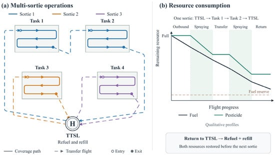
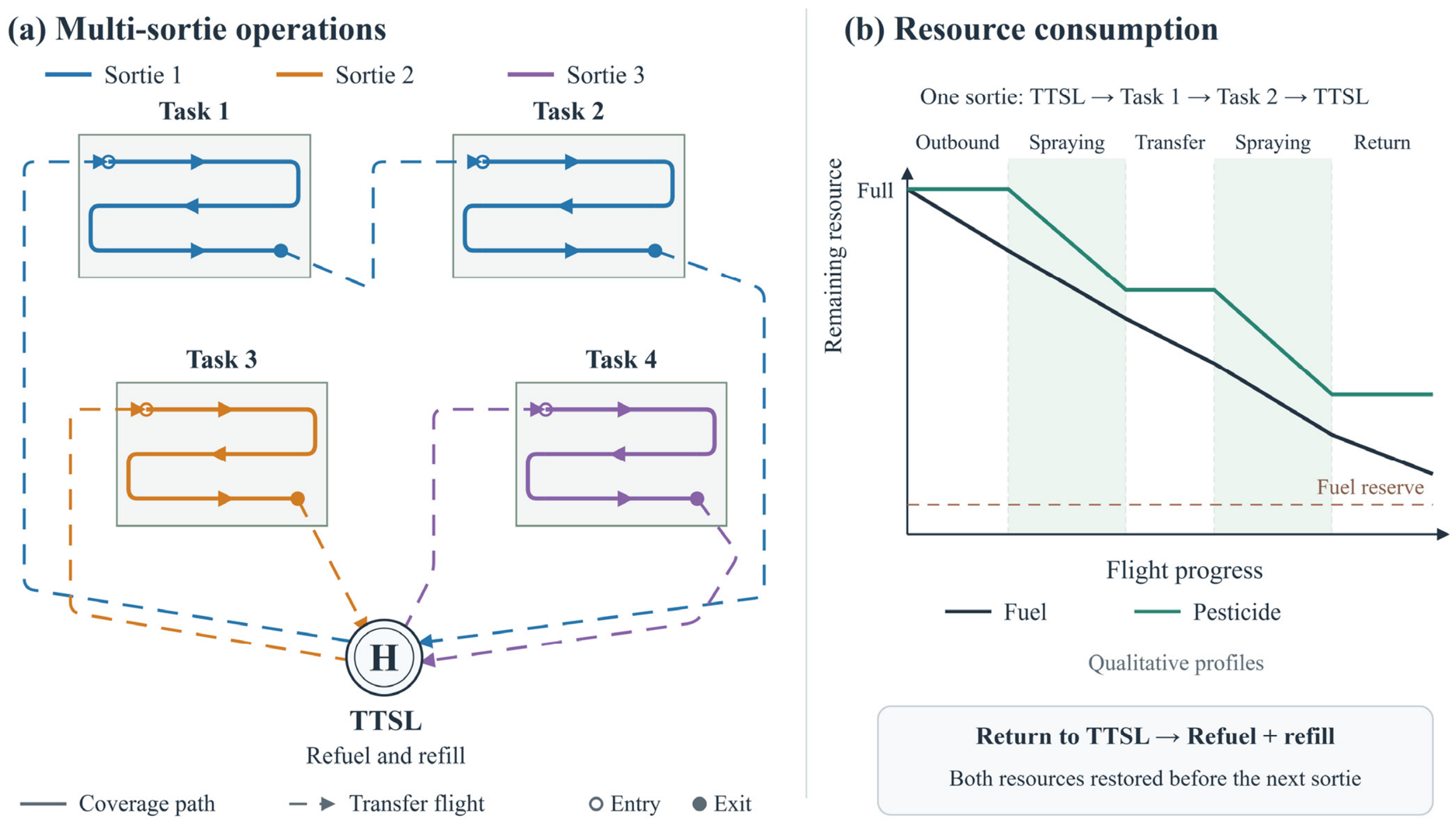
Changing task assignment changes sortie boundaries and the associated depot travel. Changing task order changes connecting distances and the pesticide and fuel masses carried on later flight segments. Therefore, total fuel cost cannot generally be evaluated using a fixed fuel cost for each task or inter-task connection. The number of sorties is determined by the task partition and is not a separate objective: a merge is beneficial only if it remains feasible and reduces total modeled fuel consumption. Section 2.2.2 specifies the fuel calculation and Section 2.3 describes the search. Figure 1 illustrates the sortie structure and resource-consumption processes. A consolidated list of symbols is provided in Supplementary Material S1.

Figure 1. Multi-sortie spraying operations and pesticide and fuel consumption.

2.2. Coverage-Task and Fuel-Consumption Modeling

The workflow separates coverage preprocessing from sortie optimization. Preprocessing fixes each task’s scanning direction, traversal variant, entry/exit points, ordered spraying segments, and prescribed internal connections. Any split needed to respect pesticide capacity is also completed at this stage. The scheduling search then changes only the grouping of these tasks into sorties and their order within each sortie, while the TTSL and flight speed remain fixed. Inter-task and depot connections are determined by those sequence decisions. Coverage-path generation is therefore an input to the optimization, whereas resource-feasible routing of the resulting tasks is the decision problem of the optimization.

2.2.1. VMM-Based Coverage-Task Generation

Coverage-task generation adapts the VMM approach used in earlier helicopter spraying studies [11,12]. Irregular forest polygons are first preprocessed by convex decomposition. The decomposition uses recursive triangulation and intersection with the input polygon, followed by greedy merging of adjacent pieces when their union satisfies the convexity criterion. The intended partition has non-overlapping interiors, while adjacent subregions may share boundaries. Convexity is assessed using an area-difference tolerance of 0.01 m² between a polygon and its convex hull. Intersection fragments smaller than 1 m² are discarded. Each retained subregion is subsequently processed as a candidate coverage task.

For a subregion P_i with area A_i, the scanning angle θ is searched over [0, 180^°] using NSGA-II [25]. Let D_⊥,i(θ) and $D_{\parallel }$,_i(θ) denote the spans of the subregion projected perpendicular and parallel to the scanning direction, respectively. Let w be the effective spray width. The two search objectives are the estimated number of turns T_i(θ) and a geometric excess-area proxy R_i(θ):

$$T_i(\theta )=⌈{\displaystyle \frac{D_{\perp ,i}(\theta )}{w}}⌉-1$$

(9)

$$R_i(\theta )=100\max \left\{0,{\displaystyle \frac{D_{\perp ,i}(\theta )D_{\parallel ,i}(\theta )-A_i+T_i(\theta )w^2/2}{A_i}}\right\}$$

(10)

The second objective combines the difference between the enclosing rectangle area and the subregion area with a turn-related geometric term. It is used to rank scanning directions and does not represent a measured overspray percentage. NSGA-II is run with a population of 15 for 15 generations. Among the returned nondominated candidates, the direction with the lowest estimated turn count is selected; ties are resolved by choosing the smaller value of the second objective. The selected angle is denoted by ${\theta }_i^{*}$.

Equations (9) and (10) are geometric criteria used only to select a scanning direction during preprocessing. The ceiling operation in Equation (9) estimates the number of swaths, and subtracting one gives the number of transitions between them. In Equation (10), the bounding-rectangle area and the turn-related area term are compared with the polygon area and normalized by that area; the factor 100 expresses the resulting proxy on a percentage scale. These criteria do not evaluate sortie fuel consumption. Equation (11) rotates the coordinate directions into vectors along and normal to the selected scan direction, which are then used to place the spraying strips.

The selected angle defines the scanning and normal unit vectors:

$$e_{s,i}={(\cos {\theta }_i^{*},\sin {\theta }_i^{*})}^T,\hspace{1em}\hspace{1em}{e}_{n,i}={(-\sin {\theta }_i^{*},\cos {\theta }_i^{*})}^T$$

(11)

Let u_min,i be the minimum projection of the subregion onto e_n,i. Parallel scan lines are placed at normal offsets u_min,i + (j + 1/2)w, where j = 0,…,N_i − 1 and $N_i=⌈{\displaystyle \frac{D_{\perp ,i}({\theta }_i^{*})}{w}}⌉$. The lines are intersected with the subregion polygon to obtain spraying segments, and empty intersections are discarded. Each segment is stored with its endpoints and length.

For subregions narrower than the effective spray width, the standard half-swath offset may produce no valid spraying segment. In this case, a single scan line is placed at the midpoint of the normal projection interval, without changing the physical spray width.

Up to four distinct endpoints on the first and last nonempty scan strips are selected as candidate starting points. For each starting point, the spraying segments are ordered in a boustrophedon sequence, producing a traversal variant with a specified entry point and exit point. Let $𝒱$_i be the set of variants for task i, and let $ℰ$_iv contain the spraying segments of variant v ∈ $𝒱$_i. Its pesticide demand is calculated as

$$d_{\mathit{iv}}=\lambda {\displaystyle \sum _{e\in {\mathcal{E}}_{\mathit{iv}}}{L}_e},\hspace{1em}\hspace{1em}\lambda ={\displaystyle \frac{\mathit{aw}}{{10}^4}}$$

(12)

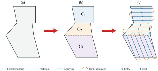
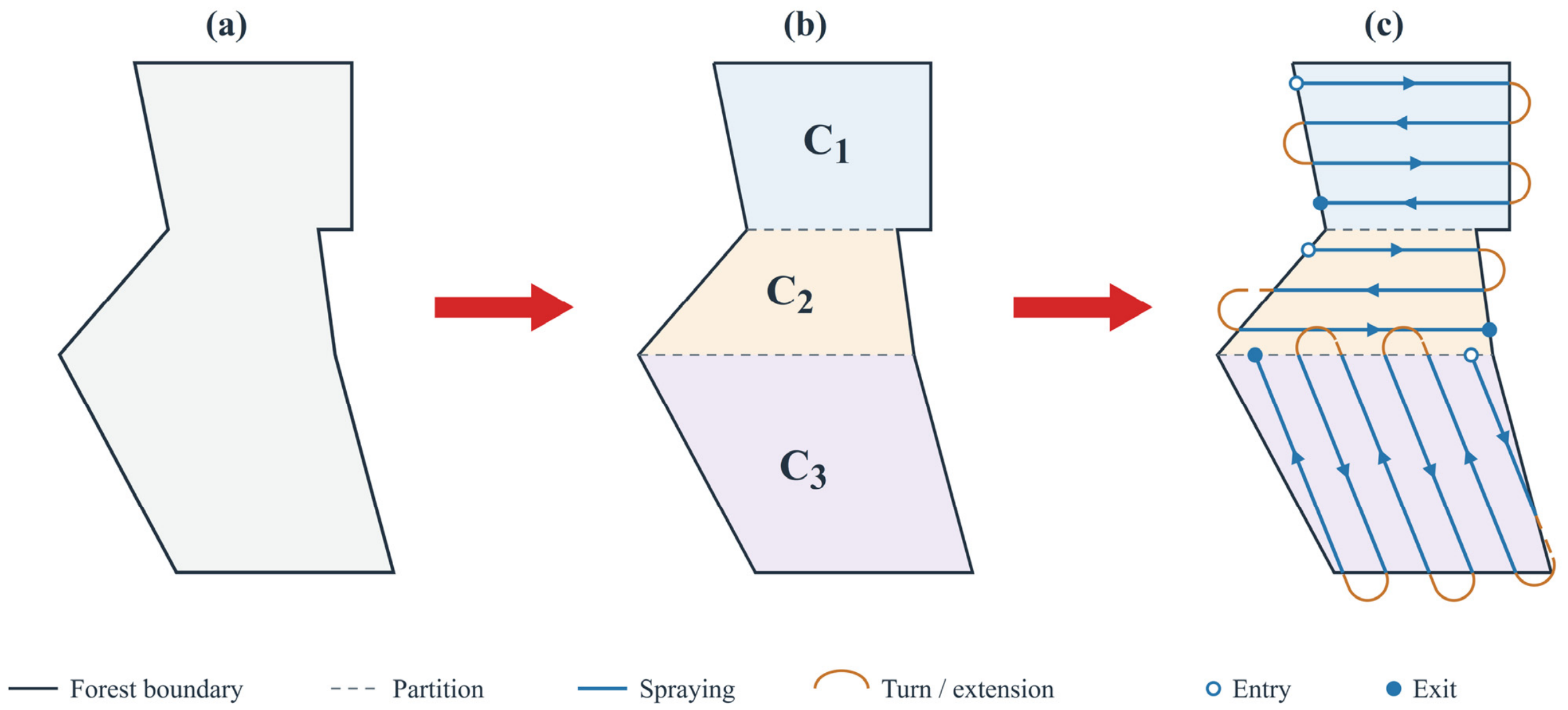
where L_e is the spraying-segment length in meters and a is the application rate in kg/ha. Thus, λ has units of kg/m. Each subregion with a generated spraying sequence forms one scheduling task. For each subregion, the candidate traversal variants are compared using the sum of spraying-segment lengths and straight-line distances connecting consecutive spraying segments. The variant with the smallest total internal distance is selected, with ties resolved by candidate index. Its entry point, exit point, and spraying-segment order are then fixed before scheduling. If the selected sequence exceeds the pesticide payload capacity, it is partitioned sequentially into capacity-feasible tasks during preprocessing. A spraying segment is split at the capacity boundary when necessary. This partitioning is not required for Forest1–Forest4, in which each convex subregion forms one scheduling task. The resulting tasks are shared by all algorithms. The scheduling procedure determines their sortie assignments and visiting order while preserving each task’s internal coverage path. Figure 2 illustrates the preprocessing procedure.

Figure 2. Schematic illustration of convex decomposition and VMM-based coverage-task generation: (a) the original irregular forest polygon; (b) the resulting convex subregions; and (c) the fixed coverage paths with task entry and exit points.

Equation (12) converts the total length of spraying segments into pesticide demand. The divisor 10⁴ converts hectares to square meters, so multiplying application rate by swath width and segment length gives kilograms. Non-spraying connections contribute no pesticide demand but still contribute flight distance and fuel consumption. Once a traversal variant has been selected, this demand is the fixed d_i used in Equation (4).

2.2.2. Fuel-Consumption Modeling

Fuel consumption is estimated using a load-dependent rotary-wing power model. The power decomposition follows Zeng et al. [26] and the helicopter power analysis of Laxman et al. [27]. Gao et al. [28] provide experimental evidence for the power–speed relationship of rotary-wing UAVs. These studies inform the power-model structure, which is coupled here with changing pesticide and fuel masses for multi-forest spraying operations of the type considered by Fang et al. [3]. The present evaluation assumes planar flight in still air at a prescribed constant speed and air density.

Let p and f denote the remaining pesticide and fuel masses, respectively, and let m₀ be the fixed mass parameter. The aircraft weight is

W = (m₀ + p + f)g

(13)

where g is gravitational acceleration. For rotor radius R_r, the rotor disk area is $A_r=\pi R_r^2$. The hover-induced velocity is

$$v_h=\sqrt{{\displaystyle \frac{W}{2\rho A_r}}}$$

(14)

where ρ is air density. For flight speed v, define the dimensionless ratio $\xi =v^2/(2v_h^2)$. The induced power is calculated as

$$P_{\mathrm{ind}}={\displaystyle \frac{\mathit{\kappa W}{v}_h}{\sqrt{\sqrt{1+{\xi }^2}+\xi }}}$$

(15)

where κ is the induced-power correction factor. This expression is evaluated using the current pesticide and fuel masses.

Let ω be rotor angular speed, U_tip = ωR_r the blade-tip speed, and s_r = n_bc_b/(πR_r) the rotor solidity, where n_b and c_b are the blade count and chord length. The blade-profile power is

$$P_{\mathrm{prof}}={\displaystyle \frac{\delta }{8}}\rho s_r{A}_r{U}_{\mathrm{tip}}^3\left(1+{\displaystyle \frac{3v^2}{U_{\mathrm{tip}}^2}}\right)$$

(16)

where δ is the blade profile–drag coefficient. The parasite power is

$$P_{\mathrm{par}}={\displaystyle \frac{1}{2}}\rho A_{\mathrm{eq}}{v}^3$$

(17)

where A_eq is the equivalent flat-plate area. Under the planar-flight assumption, the shaft power is

$$P_{\mathrm{sh}}={\displaystyle \frac{k_t}{{\eta }_m}}\left(P_{\mathrm{ind}}+P_{\mathrm{prof}}+P_{\mathrm{par}}\right)$$

(18)

where k_t accounts for tail-rotor power and η_m is transmission efficiency. With shaft power in watts and a constant specific fuel consumption b in g/kWh, the fuel mass flow rate in kg/s is

$${\dot{m}}_f(p,f)={\displaystyle \frac{b{P}_{\mathrm{sh}}(v,p,f)}{3.6\times {10}^9}}$$

(19)

The three power components have different roles: induced power represents the rotor power associated with supporting the current weight, blade-profile power represents blade drag, and parasite power represents airframe drag. At the prescribed speed, the remaining pesticide and fuel masses affect modeled induced power through the weight in Equation (13). The profile and parasite terms retain the specified aircraft and atmospheric parameters. Equation (18) combines the main-rotor terms and accounts for tail-rotor power and transmission losses; it is not an additional flight-distance penalty.

In Equation (19), the constant specific fuel consumption is given in g/kWh and shaft power is in watts. Dividing their product by 3.6 × 10⁹ converts the result into kg/s. Multiplication by a step duration in Equation (20) then gives kilograms of fuel, and Equation (21) subtracts this amount from the remaining fuel. Equation (22) adds these increments over all steps of the complete sortie, including return travel. Thus, the final fuel total is accumulated from evolving resource states rather than from distance multiplied by a constant fuel-per-distance coefficient.

Fuel consumption is accumulated along the flight path using steps no longer than 1 s, following Equation (5). For one sortie, the index k is omitted below for readability. The remaining pesticide masses at the beginning and end of step j are p_j and p_j+1, respectively. The fuel-flow function is evaluated at their midpoint, ${\overline{p}}_j=(p_j+p_{j+1})/2$, and at the beginning-of-step fuel mass f_j. The fuel consumed during that step is

$$\Delta F_j={\dot{m}}_f({\overline{p}}_j,f_j)\Delta t_j$$

(20)

and the remaining fuel is updated as

f_j+1 = f_j−ΔF_j

(21)

Here, Δt_j is shortened when necessary to reach the end of a flight segment. During spraying, the pesticide reduction is λvΔt_j, with λ defined in Section 2.2.1. Turning connections contribute through the travel time along their prescribed paths; no separate equivalent-hover fuel surcharge is added.

For sortie k, let $ℐ$_k contain its integration steps, including outbound and return travel. Its total fuel consumption is

$$F_k={\displaystyle \sum _{j\in {\mathcal{I}}_k}\Delta }{F}_j$$

(22)

Each sortie departs with the full pesticide payload and initial fuel mass specified in Section 2.1. Unused pesticide remains aboard during return travel. Feasibility checks enforce pesticide capacity, the sortie fuel budget, and the minimum remaining fuel reserve. Aircraft mass and continuous-power limits are also checked during flight-segment evaluation.

The numerical configuration uses m₀ = 400 kg, Q_max = 200 kg, F₀ = 80 kg, and F_res = 10 kg, giving F_max = 70 kg. The prescribed speed is v = 20 m/s, with ρ = 1.225 kg/m³ and g = 9.80665 m/s². The rotor parameters are R_r = 5.0292 m, a rotational speed of 404 rpm, two blades, c_b = 0.260 m, and δ = 0.014. The remaining parameters are κ = 1.10, A_eq = 0.60 m², k_t = 1.10, η_m = 0.90, and b = 315 g/kWh. The maximum gross mass and continuous shaft power are 760 kg and 152.9 kW, respectively. These settings define the numerical fuel estimates used for comparing scheduling solutions.

2.3. SC-HALNS Scheduling Framework

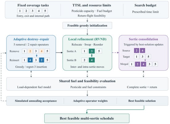
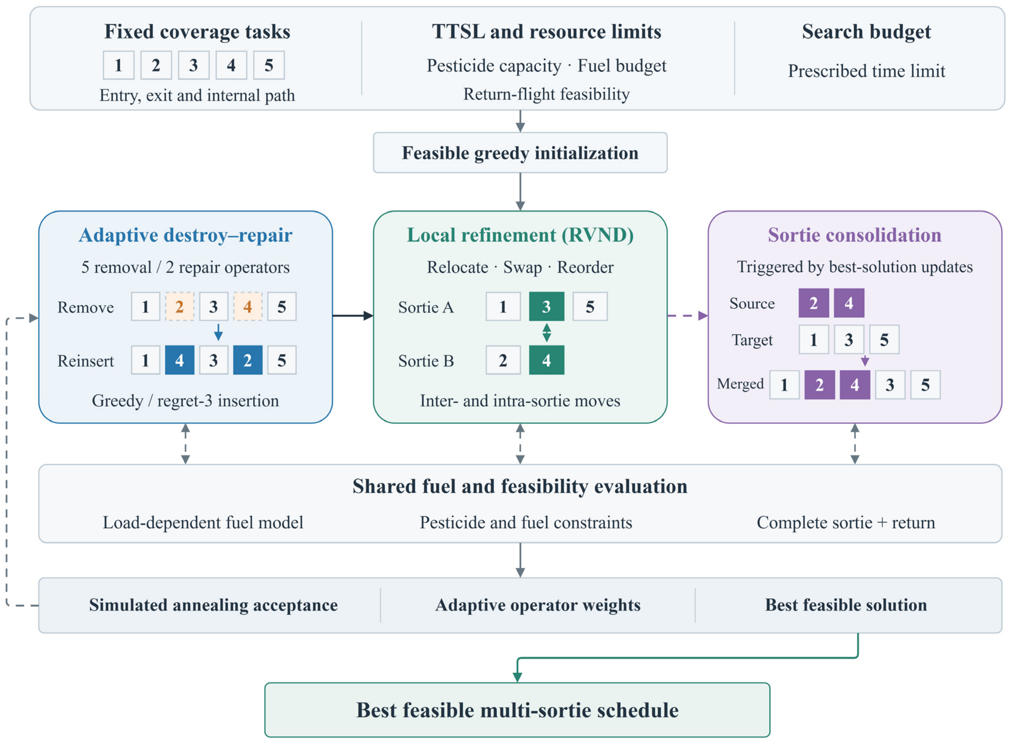
Figure 3 summarizes the SC-HALNS scheduling framework. ALNS revises task assignments and visiting orders through adaptive removal and repair, while RVND refines feasible solutions locally. SC supplements HALNS by examining whole-sortie merges that preserve feasibility and reduce total modeled fuel consumption.

Figure 3. Overview of the SC-HALNS scheduling framework.

2.3.1. Adaptive Destroy and Repair Search

A solution S consists of ordered task sequences assigned to individual sorties, with each task appearing exactly once. Let Z(S) denote its total fuel consumption. A feasible initial solution is constructed by processing tasks in a randomized order and inserting each task at the feasible position with the smallest incremental fuel consumption. Opening a new sortie is also considered. Feasibility checks account for pesticide capacity and the fuel required to complete each sortie and return to the TTSL.

Each search iteration removes a subset of tasks and reinserts them to modify task allocation and visiting order. For n assigned tasks, the removal size is sampled uniformly from the integers between 2 and max(3,⌊0.2n⌋), then capped at n. Five removal operators provide complementary search directions. Random removal samples tasks uniformly without replacement. Worst removal ranks tasks by the fuel reduction obtained by deleting each task individually from its current sortie. Shaw-related removal favors tasks with similar entry locations and pesticide demands, using a weighted sum of normalized entry-point distance and demand difference, with weights of 9 and 3, respectively. Tasks are selected successively relative to the most recently removed task, with a randomized rank bias toward greater relatedness. Zone-based removal selects the tasks whose entry points are closest to a randomly chosen anchor task. Inefficient-sortie removal prioritizes sorties with high fuel consumption per unit of assigned pesticide demand and removes tasks from them until the prescribed removal size is reached.

Two repair operators are used. Greedy repair processes removed tasks in a randomized order and selects the feasible insertion with the smallest incremental fuel consumption for each task. Regret-3 repair instead prioritizes tasks for which delaying insertion would incur a larger additional cost. For task i, let $c_i^{(k)}$ be its kth smallest feasible insertion cost and m_i the number of feasible insertion options. Its regret score is

$$r_i={\displaystyle \sum _{k=2}^{\min (3,m_i)}\left(c_i^{(k)}-c_i^{(1)}\right)}$$

(23)

Tasks with only one feasible insertion receive priority. Otherwise, the task with the largest regret score is inserted at its cheapest feasible position, with ties resolved by the smaller minimum insertion cost. Insertion options are recomputed after each placement, and both repair operators allow the creation of a new sortie. Repaired solutions are further improved by the local search and consolidation procedures described in Section 2.3.2 and Section 2.3.3.

Equation (23) measures the fuel-cost disadvantage of losing a task’s cheapest insertion position: a larger regret indicates that postponing that task may be more costly. The probabilities in Equation (24) sum to one within each operator pool. Equation (25) retains 80% of the previous weight and adds 20% of the current performance score, so selection responds to recent search outcomes without discarding the weight history.

Removal and repair operators are selected separately using adaptive roulette wheels [20,21]. Within either operator pool $𝒪$, the selection probability of operator o is

$$p_o={\displaystyle \frac{w_o}{{\displaystyle \sum _{j\in \mathcal{O}}{w}_j}}}$$

(24)

where all weights are initialized to 1. After each iteration, the weights of the selected operators are updated as

w_o ← 0.8w_o + 0.2σ

(25)

The score σ is 5 for a new best solution, 2 for an improvement over the current solution, 1 for an otherwise accepted solution, and 0 for rejection. Unselected operator weights remain unchanged.

A simulated annealing rule [29] allows occasional acceptance of a feasible solution with higher fuel consumption. For the current solution S and candidate S^′, the acceptance probability is

$$P_{\mathrm{acc}}=\min \left\{1,\exp \left[-{\displaystyle \frac{Z(S^{\prime })-Z(S)}{T(t)}}\right]\right\}$$

(26)

The temperature decreases with elapsed search time:

$$T(t)=\max \left\{{10}^{-12},0.05Z_0{(0.01)}^{\min (1,t/t_{\max })}\right\}$$

(27)

where Z₀ is the fuel consumption of the initial insertion solution before local improvement, t is elapsed time, and t_max is the prescribed time budget. Incomplete or infeasible candidates are rejected. The best feasible solution is retained throughout the search and returned when the time budget is exhausted. The ALNS-based methods were implemented using the Python alns package [30].

Equation (26) accepts every feasible improving candidate and assigns a probability below one to a feasible worsening candidate. The difference in objective values and the temperature both have the scale of fuel mass, making the exponent dimensionless. Equation (27) reduces the temperature with elapsed search time, progressively discouraging worsening moves. This acceptance rule never overrides the feasibility constraints in Section 2.1. In Equation (28), the small positive tolerance prevents numerically negligible differences from being treated as local improvements. Equation (29) is a necessary pesticide-capacity test before a consolidation attempt; the complete merged sortie must still pass fuel, reserve, mass, and power checks and reduce the objective.

2.3.2. Randomized Variable Neighborhood Descent

Randomized variable neighborhood descent (RVND) [24] is applied to the initial feasible solution and to complete solutions generated by the repair operators. It refines task allocation and visiting order through three complementary neighborhoods while preserving the coverage path within each task.

Inter-sortie relocation removes one task from its current sortie and inserts it at a different position in another existing sortie. If the source sortie becomes empty, it is removed from the schedule. Inter-sortie exchange swaps two tasks belonging to different sorties, placing each task at the position previously occupied by the other. Intra-sortie relocation removes a task and reinserts it at another position within the same sortie. These operations preserve task coverage and allow changes in both inter-task travel and the pesticide load carried along the route.

At the beginning of each descent pass, the three neighborhoods are arranged in a random order. Candidate moves within each neighborhood are also examined in a randomized order. Each candidate is evaluated for total fuel consumption and feasibility under the pesticide-capacity and fuel constraints. For moves involving two sorties, both the source and destination sorties are checked, including their return flights to the TTSL. A first-improvement rule is used: the first feasible candidate S^′ satisfying

Z(S^′) < Z(S) − ε

(28)

replaces the current solution S, where ε = 10⁻¹⁰ is a numerical tolerance for fuel comparisons. After an accepted move, all three neighborhoods are reconsidered in a newly randomized order. If no improving move is found in the current neighborhood, the search proceeds to the next one.

Each RVND call is limited to 64 candidate evaluations across all neighborhoods, and this count is not reset after an improvement. The procedure terminates when a complete pass finds no improving move, the candidate-evaluation limit is reached, or the overall search time budget is exhausted. This bounded descent balances local refinement with continued destroy-and-repair exploration. The additional whole-sortie consolidation mechanism is described in Section 2.3.3.

2.3.3. Sortie Consolidation

SC-HALNS incorporates a sortie-consolidation operator to examine whether the tasks assigned to one sortie can be incorporated into another. Sorties with low assigned pesticide demand are examined first because they leave more capacity available for combination with other sorties. By transferring a complete task sequence in a single move, the operator can eliminate a sortie without requiring intermediate single-task relocations to be accepted.

For each consolidation scan, source sorties are ranked in ascending order of total assigned pesticide demand. Let R_a and R_b denote a source and destination sortie, respectively, and let Q(R) represent the total pesticide demand of the tasks in sortie R. A pair is considered only if

Q(R_a) + Q(R_b) ≤ Q_max

(29)

The complete task sequence of R_a is inserted as a contiguous block at a candidate position in R_b, including positions before its first task and after its last task. The internal task order of both sequences is preserved, and R_a is removed from the schedule. The resulting merged sortie starts and ends at the TTSL. Its fuel consumption is evaluated with the pesticide load updated along the route, and the fuel constraint is checked for the complete sortie, including its return flight.

Within each scan, the best feasible fuel-reducing candidate among the examined block insertions is retained, using the numerical tolerance defined in Section 2.3.2. If a scan produces an improvement and computational budget remains, the sorties are ranked again and another scan is performed. Consolidation therefore reduces the number of sorties only when it also decreases total fuel consumption. Prioritizing low-demand sorties determines the search order; total fuel consumption remains the sole acceptance objective.

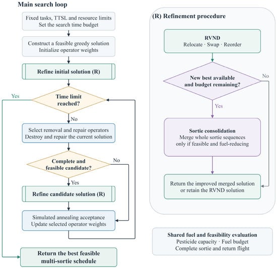
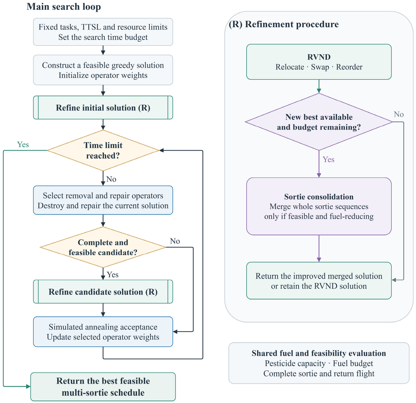
The operator is invoked after the initial RVND and subsequently when an improved best-known feasible solution becomes available at the end of an RVND call. Consolidation is applied to that best-known solution, and previously examined input schedules are skipped. Each call is limited to 128 candidate evaluations and 2 s, while cumulative consolidation time is limited to 10% of the overall search budget. A call ends when a scan yields no improvement or an applicable budget is exhausted. The best fully evaluated feasible candidate is retained. If consolidation yields no fuel reduction, the solution returned by RVND is passed to the acceptance rule in Section 2.3.1; otherwise, the improved consolidated solution is passed instead. Figure 4 shows the search flow and refinement procedure.

Figure 4. Search flow of SC-HALNS and its refinement procedure combining randomized variable neighborhood descent (RVND) with selective sortie consolidation.

3. Results

3.1. Planning Results

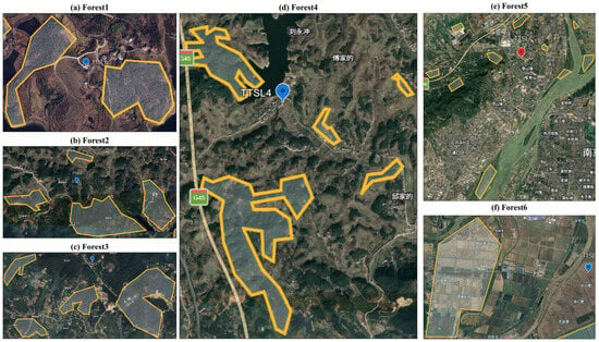
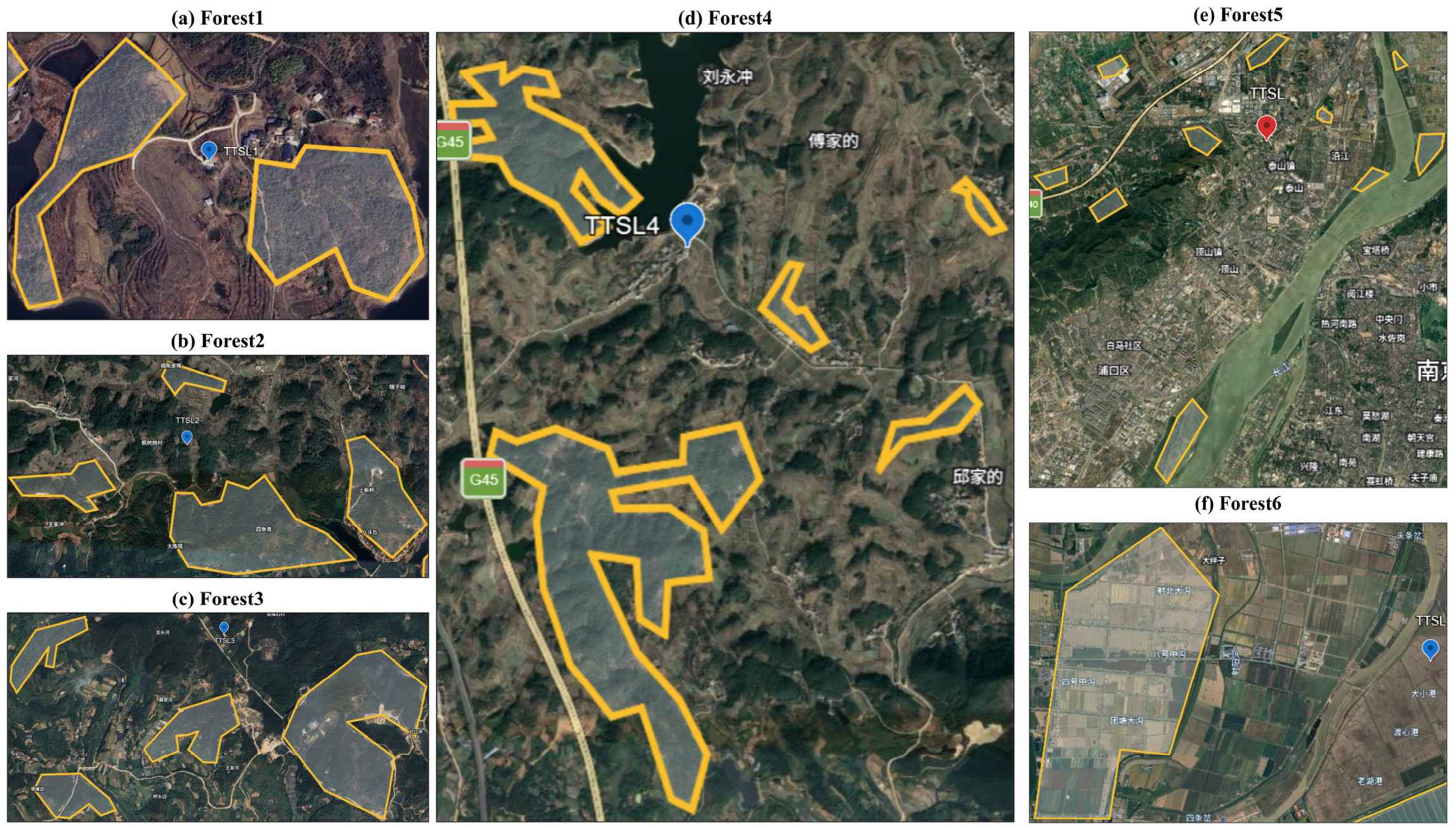
Six instances were used to evaluate the planning results. Forest1–Forest4 were constructed from GIS-derived geometries of forested areas near Wunaofeng National Park, with areas of 25.03, 45.89, 66.46, and 91.10 ha, respectively. Forest5 is located near Laoshan in Pukou District, Nanjing, and Forest6 near the mouth of the Sheyang River in Sheyang County, Yancheng. The preprocessing procedure in Section 2.2.1 generated 10, 10, 14, 31, 77, and 102 fixed coverage tasks for Forest1–Forest6, respectively. Each instance used a fixed TTSL and fixed task paths shared by all methods. The same six instances were used for the algorithm comparisons in Section 3.2. Figure 5 shows the geographic locations and boundaries of Forest1–Forest6.

Figure 5. GIS maps showing the boundaries of Forest1–Forest6. The non-English labels on the satellite imagery are place names provided by the basemap and are not related to the content of this study.

The aviation-company practice method (ACPM) was provided by Jiangsu Ningxiang Aviation Company and was used as a company-specific reference in this study. Previous studies on helicopter spraying have compared optimized routes with experience-based plans developed by pilots or planning schemes provided by an aviation company [3,12]. These studies provide a precedent for using company planning methods as practical reference baselines. ACPM and SC-HALNS were evaluated using the same fixed coverage tasks, resource constraints, and fuel-consumption model.

Table 1 summarizes modeled fuel consumption, flight distance, and sortie count. ACPM values represent its single constructed schedule, whereas SC-HALNS values are means over 20 runs. SC-HALNS obtained lower mean modeled fuel consumption and shorter mean flight distances in all six forest instances. All reported schedules satisfied the task-completion and resource constraints.

Table 1. Planning results of ACPM and SC-HALNS for six forest instances.

Forest	Method	Fuel Consumption (kg)	Flight Distance (km)	Number of Sorties
Forest1	ACPM	5.050	13.871	2.00
	SC-HALNS	4.905	13.479	2.00
Forest2	ACPM	9.724	26.615	4.00
	SC-HALNS	8.959	24.708	3.00
Forest3	ACPM	14.502	39.841	5.00
	SC-HALNS	13.673	37.524	5.00
Forest4	ACPM	22.141	60.922	7.00
	SC-HALNS	21.146	58.373	6.00
Forest5	ACPM	647.287	1787.589	77.00
	SC-HALNS	633.813	1754.683	73.00
Forest6	ACPM	737.825	2039.645	102.00
	SC-HALNS	728.183	2014.607	100.00

Note: ACPM values represent one deterministic schedule per instance. SC-HALNS values are arithmetic means over 20 runs with a nominal search budget of 100 s per run.

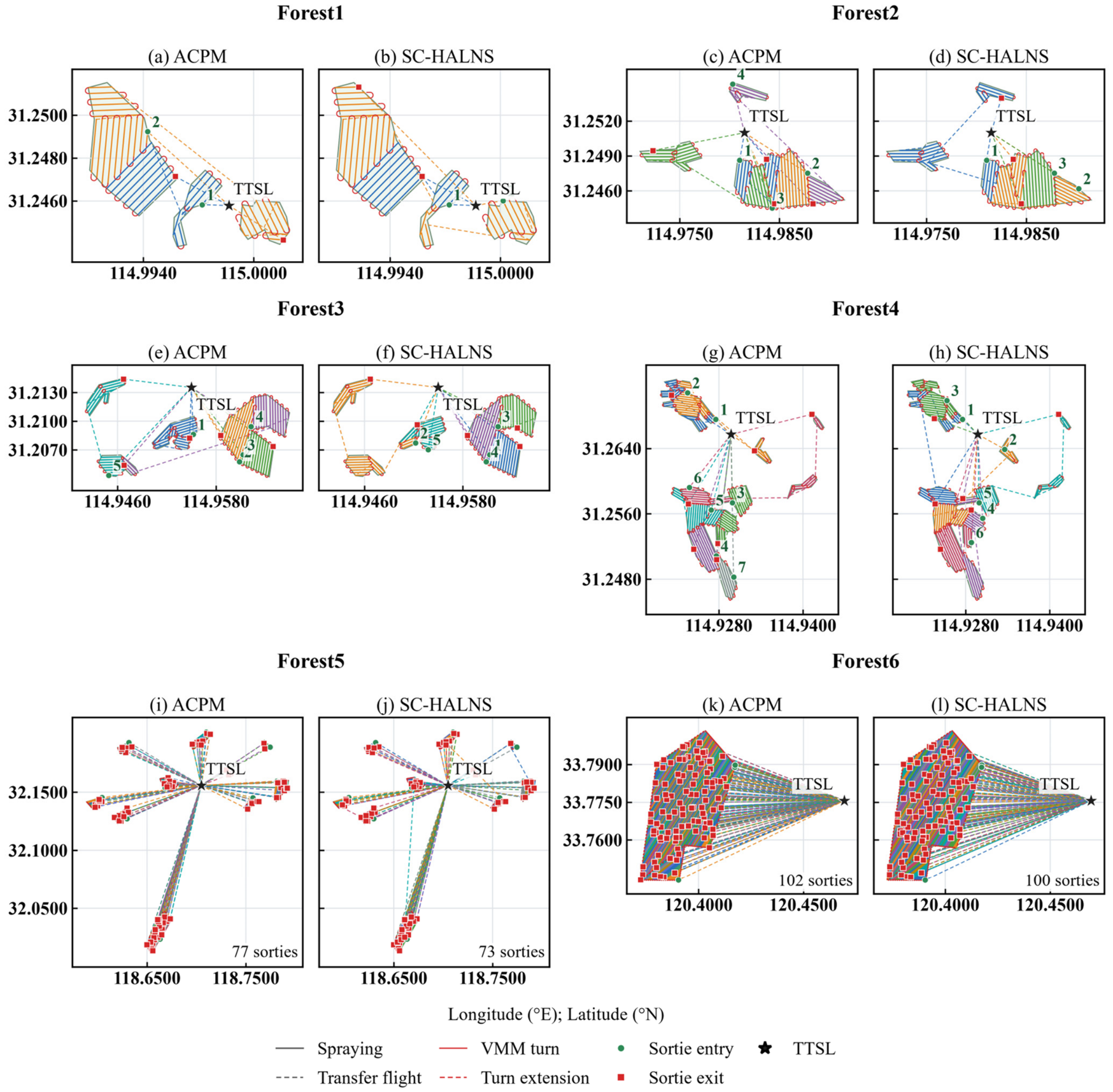
The largest relative fuel reduction occurred in Forest2, where SC-HALNS reduced the sortie count from four to three. Mean modeled fuel consumption decreased from 9.724 to 8.959 kg, and mean flight distance decreased from 26.615 to 24.708 km. In Forest1 and Forest3, fuel consumption and flight distance decreased, while the sortie counts remained at two and five, respectively. In Forest5 and Forest6, the sortie counts decreased from 77 to 73 and from 102 to 100, with mean modeled fuel reductions of 2.08% and 1.31%, respectively. Within SC-HALNS, sortie consolidation seeks to reduce the sortie count by merging task sequences, accepting a merge only when it preserves resource feasibility and lowers modeled fuel consumption. Fuel consumption can also be reduced through improved task assignments and visiting orders without changing the sortie count.

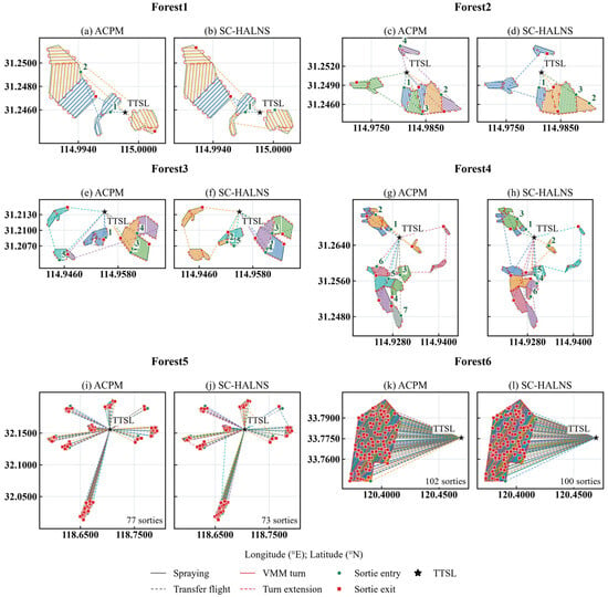
Figure 6 compares the ACPM schedules with the SC-HALNS schedules having the lowest modeled fuel consumption among 20 runs for Forest1–Forest6. The fixed coverage paths are retained, while task assignments and connecting flights differ between methods. These selected schedules illustrate the resulting sortie routes, whereas Table 1 reports mean SC-HALNS results. In Forest4, ACPM required seven sorties, while SC-HALNS used six sorties in all 20 runs. The illustrated SC-HALNS schedule consumed 20.617 kg of fuel and covered 56.915 km, compared with mean values of 21.146 kg and 58.373 km, respectively.

Figure 6. Route comparison between ACPM and SC-HALNS for Forest1–Forest6. The left panel in each pair shows the ACPM schedule, and the right panel shows the SC-HALNS schedule with the lowest modeled fuel consumption among 20 runs. Panels (a,b), (c,d), (e,f), (g,h), (i,j), and (k,l) correspond to Forest1–Forest6, respectively. Colored lines show the sortie routes, and the TTSL is marked in each panel. Numbers indicate sortie indices.

3.2. Algorithm Performance Evaluation

Algorithm performance was evaluated using the six forest instances described in Section 3.1. External comparisons included SC-HALNS, ACO-GA [31], GVNS [32], and DNIGA [11], while the internal comparison included ALNS, HALNS, and SC-HALNS. The external methods were adapted to the fixed coverage tasks and the fuel objective and resource constraints of the present problem. Each algorithm was run 20 times on each instance, with a nominal wall-clock time budget of 100 s per run. This common budget was used to compare solution quality under the same time allowance. A 100 s CPU-time limit has also been used for algorithm comparisons in a related helicopter-routing study [33]. The task sets, TTSL locations, and resource limits were fixed across methods. Table 2 and Table 3 summarize the external and ablation comparisons, respectively. They report mean modeled fuel consumption and flight distance with sample standard deviations, together with mean sortie counts.

Table 2. External comparison of SC-HALNS, ACO-GA, GVNS, and DNIGA on six forest instances.

Forest	Algorithm	Fuel Consumption (kg)	Flight Distance (km)	Mean Number of Sorties
Forest1	SC-HALNS	4.905 ± 0.004	13.479 ± 0.007	2.00
	ACO-GA	4.927 ± 0.012	13.528 ± 0.031	2.00
	GVNS	5.046 ± 0.009	13.858 ± 0.033	2.00
	DNIGA	4.922 ± 0.012	13.524 ± 0.033	2.00
Forest2	SC-HALNS	8.959 ± 0.000	24.708 ± 0.000	3.00
	ACO-GA	8.962 ± 0.013	24.716 ± 0.035	3.00
	GVNS	9.126 ± 0.099	25.150 ± 0.268	3.20
	DNIGA	8.971 ± 0.032	24.741 ± 0.085	3.00
Forest3	SC-HALNS	13.673 ± 0.000	37.524 ± 0.000	5.00
	ACO-GA	13.839 ± 0.120	37.991 ± 0.319	5.00
	GVNS	14.501 ± 0.004	39.841 ± 0.015	5.00
	DNIGA	13.847 ± 0.160	38.046 ± 0.449	5.00
Forest4	SC-HALNS	21.146 ± 0.566	58.373 ± 1.559	6.00
	ACO-GA	21.792 ± 0.207	59.991 ± 0.522	6.75
	GVNS	22.141 ± 0.000	60.922 ± 0.000	7.00
	DNIGA	25.116 ± 0.847	69.184 ± 2.275	6.75
Forest5	SC-HALNS	633.813 ± 0.000	1754.683 ± 0.000	73.00
	ACO-GA	634.161 ± 0.263	1754.740 ± 0.043	73.65
	GVNS	636.777 ± 0.412	1760.225 ± 1.175	74.75
	DNIGA	633.998 ± 0.258	1754.713 ± 0.041	73.35
Forest6	SC-HALNS	728.183 ± 0.000	2014.607 ± 0.000	100.00
	ACO-GA	728.183 ± 0.000	2014.607 ± 0.000	100.00
	GVNS	731.662 ± 2.039	2023.590 ± 5.324	100.70
	DNIGA	728.183 ± 0.000	2014.607 ± 0.000	100.00

Note: Fuel consumption and flight distance are reported as mean ± sample standard deviation over 20 runs per algorithm and instance; sortie counts are reported as means. Each run used a nominal 100 s budget. A displayed standard deviation of 0.000 may reflect variation below the rounding precision.

Table 3. Ablation comparison of ALNS, HALNS, and SC-HALNS on six forest instances.

Forest	Algorithm	Fuel Consumption (kg)	Flight Distance (km)	Mean Number of Sorties
Forest1	ALNS	4.904 ± 0.000	13.478 ± 0.000	2.00
	HALNS	4.904 ± 0.000	13.478 ± 0.000	2.00
	SC-HALNS	4.905 ± 0.004	13.479 ± 0.007	2.00
Forest2	ALNS	8.959 ± 0.000	24.708 ± 0.000	3.00
	HALNS	8.959 ± 0.000	24.708 ± 0.000	3.00
	SC-HALNS	8.959 ± 0.000	24.708 ± 0.000	3.00
Forest3	ALNS	13.673 ± 0.000	37.524 ± 0.000	5.00
	HALNS	13.673 ± 0.000	37.524 ± 0.000	5.00
	SC-HALNS	13.673 ± 0.000	37.524 ± 0.000	5.00
Forest4	ALNS	21.058 ± 0.587	58.104 ± 1.667	6.10
	HALNS	21.124 ± 0.586	58.297 ± 1.625	6.05
	SC-HALNS	21.146 ± 0.566	58.373 ± 1.559	6.00
Forest5	ALNS	633.813 ± 0.000	1754.683 ± 0.000	73.00
	HALNS	633.813 ± 0.000	1754.683 ± 0.000	73.00
	SC-HALNS	633.813 ± 0.000	1754.683 ± 0.000	73.00
Forest6	ALNS	728.183 ± 0.000	2014.607 ± 0.000	100.00
	HALNS	728.183 ± 0.000	2014.607 ± 0.000	100.00
	SC-HALNS	728.183 ± 0.000	2014.607 ± 0.000	100.00

Note: Fuel consumption and flight distance are reported as mean ± sample standard deviation over 20 runs per algorithm and instance; sortie counts are arithmetic means over the same runs. Each run used a nominal wall-clock search budget of 100 s. A displayed standard deviation of 0.000 may reflect variation below the rounding precision.

DNIGA was selected as a helicopter-spraying route-planning reference [11]. ACO-GA [31] and GVNS [32] were included to provide comparisons with hybrid population-based search and variable neighborhood search, respectively. Together, these methods allow SC-HALNS to be assessed against an application-related planning method and different search frameworks under the same fixed-task setting.

For ACO-GA, GVNS, and DNIGA, candidate solutions were encoded as task permutations and decoded into resource-feasible sorties, using a common greedy splitting procedure. A new sortie was started when appending the next task would violate feasibility under the shared evaluator. The total modeled fuel consumption of all sorties was used as the fitness value. Coverage-task paths and traversal directions remained fixed throughout the search. The reported improvements characterize the complete scheduling framework under the shared fuel model.

All experiments were executed serially on a laptop computer (MECHREVO, Tsinghua Tongfang Co., Ltd., Beijing, China) equipped with an Intel Core i7-12800HX processor and 32 GB RAM and running Windows 11. The implementations used Python 3.12.7, NumPy 2.2.6, and ALNS 7.0.0. Seeds 1001–1020 were used for the 20 runs of each algorithm on each instance. The implementation settings were kept fixed across all six instances and are summarized in Table A1.

The nominal 100 s search budget included algorithm initialization and search operations, including RVND and sortie consolidation where applicable. Common coverage-task preprocessing and final independent solution evaluation were excluded from this budget. Elapsed time was checked between computational operations. The results describe solution quality within this 100 s allowance; performance across other runtime budgets remains to be assessed.

Final modeled fuel consumption was compared using two-sided exact paired sign tests, with runs matched by seed identifier. Differences of at most 10⁻⁸ kg were treated as numerical ties and excluded from the sign counts; when all 20 pairs tied, p = 1 was reported by convention. Holm’s procedure was applied jointly to the 30 comparisons between SC-HALNS and the five comparison algorithms across the six forest instances, with a significance level of 0.05.

As shown in Table 2, SC-HALNS obtained lower mean modeled fuel consumption and shorter mean flight distance than ACO-GA, GVNS, and DNIGA in Forest1–Forest5. In Forest4, its mean fuel consumption was 21.146 kg, compared with 21.792, 22.141, and 25.116 kg for ACO-GA, GVNS, and DNIGA, respectively. The corresponding fuel reductions were 2.96%, 4.49%, and 15.81%. Mean flight distance was 58.373 km for SC-HALNS, compared with 59.991, 60.922, and 69.184 km for the three comparison algorithms. In Forest6, SC-HALNS, ACO-GA, and DNIGA obtained the same mean fuel consumption and flight distance at the reported precision. Relative to GVNS, SC-HALNS reduced these measures by 0.48% and 0.44%, respectively.

As shown in Table 3, ALNS, HALNS, and SC-HALNS obtained matching mean modeled fuel consumption and mean flight distance at the reported precision in Forest2, Forest3, Forest5, and Forest6. In Forest1, ALNS and HALNS both obtained a mean fuel consumption of 4.904 kg, compared with 4.905 kg for SC-HALNS. In Forest4, mean fuel consumption was 21.058, 21.124, and 21.146 kg for ALNS, HALNS, and SC-HALNS, respectively. The corresponding mean flight distances were 58.104, 58.297, and 58.373 km, and the mean numbers of sorties were 6.10, 6.05, and 6.00. Across the 20 seed-matched runs in Forest4, SC-HALNS obtained lower fuel consumption than HALNS in one run, the same consumption in 17 runs, and higher consumption in two runs. SC-HALNS obtained the lowest mean number of sorties in Forest4. The SC procedure provides an additional means of consolidating task sequences into fewer sorties while satisfying pesticide-capacity and fuel constraints. Fewer sorties may reduce replenishment frequency at the TTSL and the associated ground-service workload and labor costs.

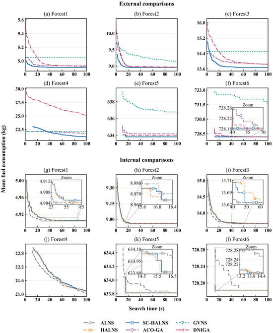
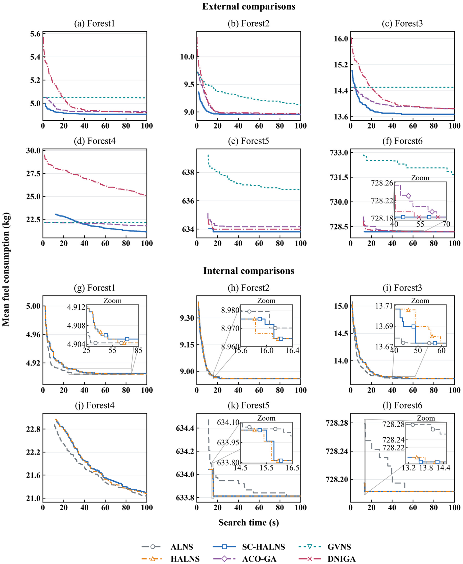
Figure 7 presents the mean best-so-far modeled fuel consumption during the 100 s search budget for the six forest instances. Each curve represents 20 independent runs, with initialization included in the elapsed time. In the external comparisons, SC-HALNS obtained the lowest terminal mean fuel consumption in Forest1–Forest5. In Forest6, it reached the same terminal level as ACO-GA and DNIGA, below that of GVNS. In the internal comparisons, ALNS, HALNS, and SC-HALNS reached the same terminal level in Forest2, Forest3, Forest5, and Forest6. In Forest5 and Forest6, the HALNS and SC-HALNS mean curves reached their final plateaus by approximately 16 and 14 s, respectively. ALNS reached these plateaus at approximately 86 and 52 s.

Figure 7. Mean best-so-far modeled fuel consumption over 100 s for Forest1–Forest6. Panels (a–f) show external comparisons, and panels (g–l) show internal comparisons. Insets magnify selected regions in panels (f,g,h,i,k,l); symbols distinguish overlapping curves. Vertical scales vary by panel.

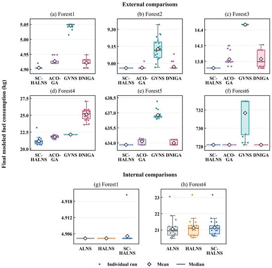
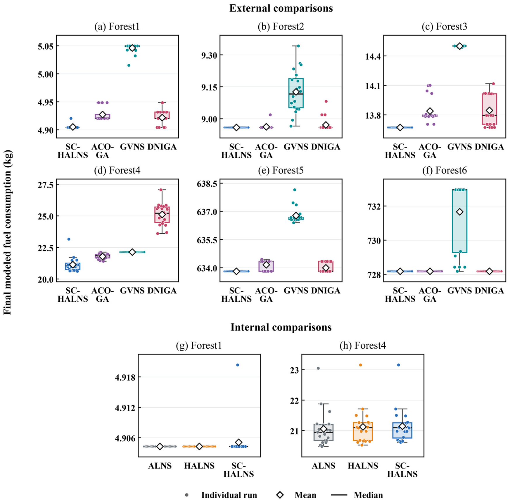
Figure 8 shows the distributions of final modeled fuel consumption over 20 runs per algorithm and forest instance. SC-HALNS produced tightly concentrated results in Forest1–Forest3, Forest5, and Forest6. In Forest6, its distribution coincided with those of ACO-GA and DNIGA at the reported precision. Internal comparison boxplots are presented for Forest1 and Forest4. For Forest2, Forest3, Forest5, and Forest6, ALNS, HALNS, and SC-HALNS obtained the same final fuel values at the reported precision across all 20 runs; these results are summarized in Table 3. In Forest4, the ALNS, HALNS, and SC-HALNS distributions overlapped, with sample standard deviations of 0.587, 0.586, and 0.566 kg, respectively.

Figure 8. Distributions of final modeled fuel consumption over 20 runs per algorithm and instance with a 100 s search budget. Panels (a–f) show external comparisons for Forest1–Forest6, respectively, and panels (g,h) show internal comparisons for Forest1 and Forest4, respectively.

After Holm adjustment, the paired tests favored SC-HALNS in 13 of the 18 external comparisons (adjusted p ≤ 0.0044): against all three external algorithms in Forest1, Forest3, and Forest4; against GVNS in Forest2 and Forest6; and against ACO-GA and GVNS in Forest5. In the internal comparisons, the adjusted p-values ranged from 0.662 to 1.000. The sortie-consolidation behavior of SC is further examined in Section 3.3. The complete statistical test results are provided in Table A2. These comparisons assess relative performance under the specified model and computational budget; no optimality gap is reported.

3.3. Analysis of Sortie Consolidation

The SC procedure was examined using the operation logs of 20 SC-HALNS runs on each forest instance. Within the prescribed budgets, SC examines previously unchecked historical best solutions following RVND, including during initialization. It inserts the entire task sequence of one sortie into another, screening candidates against the 200 kg pesticide-capacity limit. A merge is accepted when the combined sortie satisfies the resource constraints and reduces the total modeled fuel consumption of the input plan. Table 4 summarizes SC calls, candidate evaluations, accepted merges, local fuel reductions, and SC execution time, which was included in the 100 s search budget. These records describe changes to individual SC input plans; the final algorithm comparison is reported separately in Table 3.

Table 4. Whole-sortie consolidation statistics over 20 SC-HALNS runs per forest instance.

Forest	SC Calls	Candidate Evaluations	Accepted Merges	Local Fuel Reduction (kg)	Mean SC Time (s)
Forest1	97	0	0	0.000	0.000093
Forest2	101	36	5	1.418	0.027570
Forest3	167	0	0	0.000	0.000204
Forest4	317	34	4	1.032	0.023579
Forest5	60	8	2	3.611	0.015814
Forest6	33	0	0	0.000	0.003273

Note: SC calls include scans that terminate after capacity screening. Candidate evaluations count proposed merged plans submitted to the fuel evaluator. Counts and local fuel reductions are totals over 20 runs; SC time is the mean cumulative time per run. Each accepted merge removed one sortie. Local fuel reduction is measured relative to the input plan of each accepted SC call.

Accepted merges occurred in 5 of 20 runs in Forest2, 3 of 20 in Forest4, and 2 of 20 in Forest5. The mean cumulative SC time was below 0.028 s per run in each instance. For example, an accepted merge in Forest4 reduced an intermediate solution from seven to six sorties and its modeled fuel consumption from 22.357 to 21.778 kg. The merged sortie required 176.986 kg of pesticide and 3.007 kg of modeled fuel, satisfying the 200 kg capacity and 70 kg fuel-use constraints. These records illustrate how SC uses available capacity to consolidate feasible sorties. Fewer returns to the TTSL can reduce the number of replenishment cycles and may lower the associated ground-service workload and labor costs.

3.4. Sensitivity Analysis

On Forest4, flight speed, pesticide capacity, and application rate were varied individually by ±10% around 20 m/s, 200 kg, and 12 kg/ha, respectively. HALNS and SC-HALNS were run five times per setting, with a nominal 100 s search budget per run. Other parameters and coverage paths were fixed, and full-load departure was retained (Table 5).

Table 5. Sensitivity of modeled fuel consumption and sortie count in Forest4.

Setting	HALNS Fuel (kg)	SC-HALNS Fuel (kg)	Mean Sorties
Baseline	21.059 ± 0.433	21.187 ± 0.313	6
Flight speed: 18 m/s	23.538 ± 0.245	23.518 ± 0.260	6
Flight speed: 22 m/s	19.057 ± 0.364	19.152 ± 0.328	6
Pesticide capacity: 180 kg	21.268 ± 0.232	21.268 ± 0.232	7
Pesticide capacity: 220 kg	21.041 ± 0.539	21.041 ± 0.539	6
Application rate: 10.8 kg/ha	20.801 ± 0.350	20.801 ± 0.350	6
Application rate: 13.2 kg/ha	21.452 ± 0.298	21.397 ± 0.199	7

Note: Fuel values are means ± sample standard deviations over five runs. Mean sorties are identical for both algorithms.

For SC-HALNS, mean modeled fuel consumption changed by +11.01% at 18 m/s and −9.61% at 22 m/s relative to the baseline. Reducing pesticide capacity to 180 kg or increasing the application rate to 13.2 kg/ha increased mean sorties from six to seven for both algorithms. Reevaluating the ten baseline plans at fuel reserves of 5, 10, and 15 kg preserved feasibility and modeled fuel consumption.

4. Discussion

4.1. Deployment Feasibility

The six-instance results support the use of SC-HALNS for offline planning of forestry helicopter spraying. Using GIS-derived coverage tasks, it generated feasible schedules under pesticide-capacity and fuel constraints, with lower mean modeled fuel consumption and shorter mean flight distances than ACPM.

In an operational workflow, GIS boundaries and the TTSL location would support coverage-task generation and sortie scheduling. Operational personnel would review the plans for terrain, obstacles, weather, and aircraft operating requirements before transfer to a compatible navigation system.

4.2. Management Insights

Fuel-efficient scheduling should consider task allocation and visiting order alongside sortie count. In Forest1 and Forest3, SC-HALNS obtained lower mean modeled fuel consumption and shorter mean flight distances than ACPM, without changing the number of sorties.

SC serves as a supplementary procedure within HALNS, using available pesticide capacity to consolidate whole sorties while respecting fuel constraints. Accepted merges in Forest2, Forest4, and Forest5 illustrate this role (Table 4). Fewer returns to the TTSL can reduce replenishment cycles and may lower ground support workload and associated labor costs.

Merge opportunities depend on task demands and the resource requirements of the resulting routes. Each accepted merge preserves feasibility and reduces modeled fuel consumption relative to its input plan. In the Forest4 sensitivity tests, reduced pesticide capacity or increased application rate resulted in higher mean sortie counts (Table 5), illustrating how operating conditions affect replenishment needs.

4.3. Limitations and Future Work

The evaluation covers six forest instances under a numerical fuel model assuming planar flight in still air at a prescribed speed. The absolute fuel values are conditional model estimates; aircraft-specific flight measurements are needed for calibration and quantitative prediction–error assessment. Further extensions could represent terrain-following flight, variable weather, liquid sloshing [34], and center-of-gravity changes. Exact reference solutions for smaller instances and matched objective comparisons could further assess solution quality and the fuel formulation’s contribution.

Coverage paths and their entry/exit points are selected during preprocessing and remain fixed during sortie scheduling. Future work could jointly optimize entry/exit choices, task allocation, and visiting order. Broader tests across task distributions, TTSL locations, and search parameter settings could assess the framework’s applicability and clarify the conditions favoring consolidation.

Cooperative spraying with manned helicopters and UAVs could also be explored, assigning coverage tasks according to platform-specific paths, payload capacities, endurance, and operating costs, particularly for small or isolated subregions.

5. Conclusions

This study developed SC-HALNS for fuel-efficient multi-sortie forestry helicopter spraying under pesticide-capacity and fuel constraints. Fixed GIS-derived coverage tasks and a load-dependent fuel model support task allocation and visiting-order optimization. HALNS combines adaptive destroy-and-repair search with randomized variable neighborhood descent; SC supplements this framework by consolidating whole sorties when a merge preserves feasibility and reduces total modeled fuel consumption.

Across six forest instances, SC-HALNS obtained lower mean modeled fuel consumption and shorter mean flight distances than ACPM. Consolidation records showed feasible reductions in sortie count and returns to the TTSL in intermediate plans. Fewer returns may reduce replenishment workload and associated labor costs. These results support offline planning under the evaluated model assumptions.

References

- Chen, H.; Lan, Y.; Fritz, B.K.; Hoffmann, W.C.; Liu, S. Review of agricultural spraying technologies for plant protection using unmanned aerial vehicle (UAV). Int. J. Agric. Biol. Eng. 2021, 14, 38–49. [Google Scholar] [CrossRef] [Scilit]
- Zheng, J.; Xu, Y. A review: Development of plant protection methods and advances in pesticide application technology in agro-forestry production. Agriculture 2023, 13, 2165. [Google Scholar] [CrossRef] [Scilit]
- Fang, S.; Ru, Y.; Liu, Y.; Hu, C.; Chen, X.; Liu, B. Route planning of helicopters spraying operations in multiple forest areas. Forests 2021, 12, 1658. [Google Scholar] [CrossRef] [Scilit]
- Cabreira, T.M.; Brisolara, L.B.; Ferreira, P.R., Jr. Survey on coverage path planning with unmanned aerial vehicles. Drones 2019, 3, 4. [Google Scholar] [CrossRef] [Scilit]
- Apostolidis, S.D.; Kapoutsis, P.C.; Kapoutsis, A.C.; Kosmatopoulos, E.B. Cooperative multi-UAV coverage mission planning platform for remote sensing applications. Auton. Robot. 2022, 46, 373–400. [Google Scholar] [CrossRef] [Scilit]
- Oksanen, T.; Visala, A. Coverage path planning algorithms for agricultural field machines. J. Field Robot. 2009, 26, 651–668. [Google Scholar] [CrossRef] [Scilit]
- Torres, M.; Pelta, D.A.; Verdegay, J.L.; Torres, J.C. Coverage path planning with unmanned aerial vehicles for 3D terrain reconstruction. Expert Syst. Appl. 2016, 55, 441–451. [Google Scholar] [CrossRef] [Scilit]
- Choset, H.; Pignon, P. Coverage path planning: The boustrophedon decomposition. In Proceedings of the 1st International Conference on Field and Service Robotics, Canberra, Australia, 8–10 December 1997; pp. 216–222. Available online: https://publications.ri.cmu.edu/coverage-path-planning-the-boustrophedon-decomposition (accessed on 28 September 2026).
- Li, J.; Sheng, H.; Zhang, J.; Zhang, H. Coverage path planning method for agricultural spraying UAV in arbitrary polygon area. Aerospace 2023, 10, 755. [Google Scholar] [CrossRef] [Scilit]
- Wang, L.; Zhuang, X.; Zhang, W.; Cheng, J.; Zhang, T. Coverage path planning for UAVs: An energy-efficient method in convex and non-convex mixed regions. Drones 2024, 8, 776. [Google Scholar] [CrossRef] [Scilit]
- Fang, S.; Ru, Y.; Hu, C.; Liu, Y.; Liu, B.; Li, J.; Xia, D. Route planning for multi-forest areas of helicopter plant protection operations based on vector modeling method and double-layer nested improved genetic algorithm. Trans. Chin. Soc. Agric. Eng. 2022, 38, 70–79, (In Chinese with English abstract). [Google Scholar] [CrossRef]
- Fang, S.; Ru, Y.; Hu, C.; Yang, F. Planning of takeoff/landing site location, dispatch route, and spraying route for a pesticide application helicopter. Eur. J. Agron. 2023, 146, 126814. [Google Scholar] [CrossRef] [Scilit]
- Fang, S.; Ru, Y.; Hu, C.; Yang, F.; Xue, J.; Zhou, J. Planning the temporary takeoff/landing site’s location for a pesticide spraying helicopter based on an intelligent fusion algorithm. Comput. Electron. Agric. 2023, 209, 107826. [Google Scholar] [CrossRef] [Scilit]
- Yu, S.; Zhu, J.; Shen, J.; Yang, X.; Wang, P. A three-dimensional full-coverage operation path planning method for plant protection unmanned aerial vehicles based on energy consumption modeling. Electronics 2023, 12, 4051. [Google Scholar] [CrossRef] [Scilit]
- Lara-Molina, F.A. Optimization of coverage path planning for agricultural drones in weed-infested fields using semantic segmentation. Agriculture 2025, 15, 1262. [Google Scholar] [CrossRef] [Scilit]
- Cattaruzza, D.; Absi, N.; Feillet, D. Vehicle routing problems with multiple trips. 4OR 2016, 14, 223–259. [Google Scholar] [CrossRef] [Scilit]
- Cattaruzza, D.; Absi, N.; Feillet, D.; Vidal, T. A memetic algorithm for the Multi Trip Vehicle Routing Problem. Eur. J. Oper. Res. 2014, 236, 833–848. [Google Scholar] [CrossRef] [Scilit]
- Bektaş, T.; Laporte, G. The Pollution-Routing Problem. Transp. Res. Part B Methodol. 2011, 45, 1232–1250. [Google Scholar] [CrossRef] [Scilit]
- Demir, E.; Bektaş, T.; Laporte, G. An adaptive large neighborhood search heuristic for the Pollution-Routing Problem. Eur. J. Oper. Res. 2012, 223, 346–359. [Google Scholar] [CrossRef] [Scilit]
- Ropke, S.; Pisinger, D. An adaptive large neighborhood search heuristic for the pickup and delivery problem with time windows. Transp. Sci. 2006, 40, 455–472. [Google Scholar] [CrossRef] [Scilit]
- Pisinger, D.; Ropke, S. A general heuristic for vehicle routing problems. Comput. Oper. Res. 2007, 34, 2403–2435. [Google Scholar] [CrossRef] [Scilit]
- Windras Mara, S.T.; Norcahyo, R.; Jodiawan, P.; Lusiantoro, L.; Rifai, A.P. A survey of adaptive large neighborhood search algorithms and applications. Comput. Oper. Res. 2022, 146, 105903. [Google Scholar] [CrossRef] [Scilit]
- Voigt, S. A review and ranking of operators in adaptive large neighborhood search for vehicle routing problems. Eur. J. Oper. Res. 2025, 322, 357–375. [Google Scholar] [CrossRef] [Scilit]
- Penna, P.H.V.; Subramanian, A.; Ochi, L.S. An iterated local search heuristic for the heterogeneous fleet vehicle routing problem. J. Heuristics 2013, 19, 201–232. [Google Scholar] [CrossRef] [Scilit]
- Deb, K.; Pratap, A.; Agarwal, S.; Meyarivan, T. A fast and elitist multiobjective genetic algorithm: NSGA-II. IEEE Trans. Evol. Comput. 2002, 6, 182–197. [Google Scholar] [CrossRef] [Scilit]
- Zeng, Y.; Xu, J.; Zhang, R. Energy minimization for wireless communication with rotary-wing UAV. IEEE Trans. Wirel. Commun. 2019, 18, 2329–2345. [Google Scholar] [CrossRef] [Scilit]
- Laxman, V.; Lim, J.-H.; Shin, S.-J.; Ko, K.-H.; Jung, S.-N. Power and trim estimation for helicopter sizing and performance analysis. Int. J. Aeronaut. Space Sci. 2011, 12, 156–162. [Google Scholar] [CrossRef] [Scilit][Green Version]
- Gao, N.; Zeng, Y.; Wang, J.; Wu, D.; Zhang, C.; Song, Q.; Qian, J.; Jin, S. Energy model for UAV communications: Experimental validation and model generalization. China Commun. 2021, 18, 253–264. [Google Scholar] [CrossRef] [Scilit]
- Kirkpatrick, S.; Gelatt, C.D., Jr.; Vecchi, M.P. Optimization by simulated annealing. Science 1983, 220, 671–680. [Google Scholar] [CrossRef] [Scilit] [PubMed]
- Wouda, N.A.; Lan, L. ALNS: A Python implementation of the adaptive large neighbourhood search metaheuristic. J. Open Source Softw. 2023, 8, 5028. [Google Scholar] [CrossRef] [Scilit]
- Chen, X.; Wu, Y.; Xu, S. Mission planning of UAVs and UGV for building inspection in rural area. Algorithms 2024, 17, 177. [Google Scholar] [CrossRef] [Scilit]
- Papalitsas, C.; Karakostas, P.; Andronikos, T.; Sioutas, S.; Giannakis, K. Combinatorial GVNS (General Variable Neighborhood Search) optimization for dynamic garbage collection. Algorithms 2018, 11, 38. [Google Scholar] [CrossRef] [Scilit]
- Yang, K.; Duan, P.; Yu, H. An improved genetic algorithm for solving the helicopter routing problem with time window in post-disaster rescue. Math. Biosci. Eng. 2023, 20, 15672–15707. [Google Scholar] [CrossRef] [Scilit] [PubMed]
- Ru, Y.; Xue, J.; Liu, B.; Fang, S.; Hu, C.; Zhou, J. Simulation and experiment of the anti-shake damping of liquid in helicopter application tank. Trans. Chin. Soc. Agric. Eng. 2023, 39, 55–63, (In Chinese with English abstract). [Google Scholar] [CrossRef]
Disclaimer/Publisher’s Note: The statements, opinions and data contained in all publications are solely those of the individual author(s) and contributor(s) and not of MDPI and/or the editor(s). MDPI and/or the editor(s) disclaim responsibility for any injury to people or property resulting from any ideas, methods, instructions or products referred to in the content. |
© 2026 by the authors. Licensee MDPI, Basel, Switzerland. This article is an open access article distributed under the terms and conditions of the Creative Commons Attribution (CC BY) license.