Online Automated Clamping Error Compensation for Robotic Grinding of Turbine Blade Thermal Barrier Coatings via Reference Point Cloud Registration

Abstract

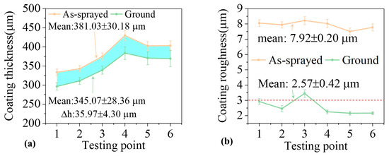
This paper presents an automated clamping error compensation method for robotic grinding of thermal barrier coatings (TBCs) on turbine blades. In the eye-to-hand robotic grinding cell, a fixed line-laser scanner acquires a point cloud after each blade pickup. The key innovation is a reference-scan strategy: the first blade in a batch is calibrated once with manual assistance, and its scanned point cloud is stored as the reference, against which every subsequent pickup is localized by Trimmed-ICP fine registration. Because the clamping error is mechanically bounded and lies inside the ICP convergence basin, coarse registration is entirely bypassed, enabling fully automated batch production. An error propagation model demonstrates that the proposed compensation decouples the random per-pickup clamping error from the systematic error budget. Experiments over 530 pickup trials across four blade types achieve a mean compensation rate of 91%, post-compensation residuals below 0.2 mm, and a valid-registration rate of 98.5% (530 of 538 records) with no solver failures. Batch validation on 118 T1 blades confirmed uniform coating removal (35.97 ± 4.30 μm) and a reduction in surface roughness from Ra 7.92 μm to 2.57 μm, with the Ra ≤ 3.0 μm limit met at five of six measurement locations.

1. Introduction

Turbine blades operate under extreme thermo-mechanical conditions in gas turbine engines. Thermal barrier coatings (TBCs), as one of the key nanoscale material technologies applied to aero-engine hot-section components including turbine blades, combustion chambers, and thermal protection systems, play an increasingly critical role in extending component service life and reliability [1]. To protect the blade substrate from high-temperature oxidation and thermal fatigue, TBCs are deposited onto the blade surface via thermal spraying processes such as atmospheric plasma spraying (APS) or electron-beam physical vapor deposition (EB-PVD). However, as-sprayed coatings exhibit rough surface topography and geometric deviations from the nominal blade profile. Robotic belt grinding or abrasive wheel grinding is therefore employed as a post-processing step to restore the required aerodynamic profile and surface finish [2,3,4]. The accuracy of robotic grinding critically depends on the precise spatial relationship between the robot end-effector, the grinding tool, and the workpiece. Any deviation in the workpiece localization translates directly into trajectory errors on the blade surface, potentially causing non-uniform coating removal, under-grinding, or over-grinding, all of which compromise the thermal barrier performance [5,6].

In a typical robotic grinding cell for turbine blades, a line-laser profilometer is integrated in a fixed position (eye-to-hand configuration) to serve as the primary metrology sensor. The overall calibration pipeline consists of three stages: (a) hand–eye calibration to determine the rigid transformation between the line-laser coordinate frame and the robot base frame [7]; (b) blade pose calibration to localize the blade workpiece in the robot base frame through point cloud registration with the blade CAD model; and (c) trajectory generation, remapping, and execution [5,6,8].

Hand-eye calibration for 2D/3D laser scanners in eye-to-hand or eye-in-hand configurations has been extensively studied using various calibration targets. Standard spheres [9,10] are the most widely adopted because their geometry is invariant under arbitrary viewing directions, making sphere center extraction robust. Chessboard patterns [11] and planar features [12] are also used but require multi-view constraints. In this work, the ball-based method [7,9] is adopted as the prerequisite hand–eye calibration step.

Blade pose calibration relies on point cloud registration, which is typically divided into coarse and fine phases. Coarse registration aims to align two point clouds with unknown, potentially large, initial poses. Representative methods include global feature-based methods such as Sample Consensus Initial Alignment (SAC-IA) [13] using Fast Point Feature Histograms (FPFH) [14], four-point congruent set methods including 4PCS [15] and its accelerated variant Super4PCS [16], and globally optimal registration methods such as Go-ICP [17] using branch-and-bound optimization and TEASER++ [18] using truncated least squares with robust estimation. While these methods perform well on object-rich scenes, their reliability degrades on smooth, feature-sparse surfaces such as turbine blade airfoils, where local geometric descriptors lack distinctiveness and symmetry-induced ambiguities frequently lead to incorrect correspondences. Fine registration refines an approximate initial alignment to high precision. The Iterative Closest Point (ICP) algorithm [19] and its variants, point-to-plane ICP [20], Generalized ICP (GICP) [21], and Normal ICP (NICP) [22], are widely regarded as the standards in both research and industry. ICP is known to converge reliably when the initial misalignment is within its convergence basin, typically up to approximately 30° in rotation and a translation commensurate with the correspondence search radius [23].

Despite the maturity of these calibration techniques, a critical practical bottleneck arises during batch production. In industrial practice, turbine blades are loaded into dedicated fixtures and placed in bins. A pneumatic gripper mounted on the robot end-effector picks up each blade-fixture assembly sequentially. Due to mechanical clearances in the fixture, gripper positioning repeatability limits, and slight variations in the gripping posture, each pickup introduces a non-negligible clamping error, whose magnitude is set by the tolerances of the fixture and gripper and increases as they wear. These errors, if left uncorrected, degrade grinding accuracy to an unacceptable level. The conventional remedy is to repeat the full calibration pipeline (coarse and fine registration) for every blade after each pickup. This requires manual intervention for coarse registration, because fully automatic coarse registration remains unreliable on smooth free-form blade surfaces. Consequently, the production line cannot operate in a fully automated manner.

Error compensation in robotic machining has been approached from several complementary perspectives, but none fully resolves this bottleneck. Kinematic calibration [24,25] identifies and compensates for robot geometric parameter errors through external measurements. However, it is typically performed offline and does not account for workpiece-dependent variations such as clamping inconsistencies. Force-controlled compensation [26,27] employs force/torque sensors for real-time trajectory adjustment; this approach is effective for maintaining consistent contact force during grinding but cannot directly correct geometric misalignment independent of the contact state. Vision-based compensation has utilized laser trackers [28] or stereo cameras [29] for online or intermittent workpiece localization; however, these approaches either require expensive additional hardware or target fundamentally different machining scenarios than free-form surface grinding of turbine blades. Moreover, although hand–eye calibration and blade pose calibration are well studied as standalone problems, their integration into a fully automated batch production workflow, where clamping errors must be compensated without manual intervention, has not been addressed. The specific challenge of automating turbine blade TBC grinding using only the already-integrated line-laser scanner remains unexplored.

This paper fills this gap by proposing an automated clamping error compensation method that leverages the existing line-laser scanner and requires no additional hardware. The key insight is that the clamping error is inherently bounded by mechanical constraints (fixture clearance, gripper repeatability) and therefore lies well within the convergence basin of the ICP fine registration algorithm. Consequently, if a reference point cloud is acquired during the initial (manually-assisted) calibration, subsequent blades can be localized solely by ICP-based fine registration against this reference, bypassing coarse registration entirely. Based on this insight, a three-step automated compensation procedure is executed for every blade after the initial calibration:

• Rescanning: The line-laser scans the newly picked blade, acquiring a current point cloud P_i in the scanner frame {L}.
• Fine registration: ICP is performed between P_i and the reference point cloud P_ref (both in {L}) to estimate the clamping error ΔT.
• Trajectory remapping: The grinding trajectory is transformed by ΔT before execution.

Since both point clouds are acquired by the identical sensor from the identical scanning viewpoint, they share consistent noise characteristics and sampling density, further enhancing ICP convergence stability.

The contributions and novelty of this work are threefold:

Automated clamping error compensation framework. The central methodological novelty is the reference-scan strategy that leverages the bounded nature of clamping errors to convert a manual coarse registration step into fully automated fine registration. In the proposed method, the first blade of a batch is calibrated once, and its scan is retained as a reference point cloud; every subsequent pickup is then localized by Trimmed-ICP fine registration alone, because the clamping error is mechanically bounded and therefore lies inside the convergence basin of ICP. Unlike the conventional remedy, which re-executes the coarse and fine registration pipeline after every pickup, the reference-scan strategy requires manual assistance only once per batch and thereafter registers each scan against a reference scan rather than against a mesh model.

Error propagation modeling. A comprehensive error propagation chain is derived, linking hand–eye calibration error, initial pose calibration error, and clamping error to the final grinding trajectory. The model quantitatively demonstrates that the proposed compensation effectively decouples clamping errors from the trajectory error budget. Prior compensation studies report compensation outcomes but do not decompose the residual error budget in this way.

Experimental validation. In contrast to laboratory demonstrations on individual workpieces, the method is validated on an industrial cell over 530 pickup trials on four blade types and on a batch of 118 production blades, which establishes the repeatability of the approach rather than a single best-case result.

The remainder of this paper is organized as follows. Section 2 describes the system configuration, summarizes the prerequisite calibration stages and presents the proposed automated clamping error compensation method in detail. Section 3 reports experimental results. Section 4 discusses the error propagation model. Section 5 concludes this paper and discusses future work.

2. System Architecture and Calibration Prerequisites

2.1. System Components and Coordinate Frames

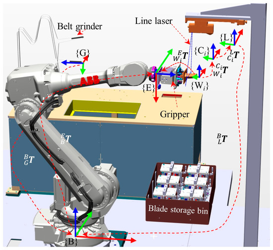
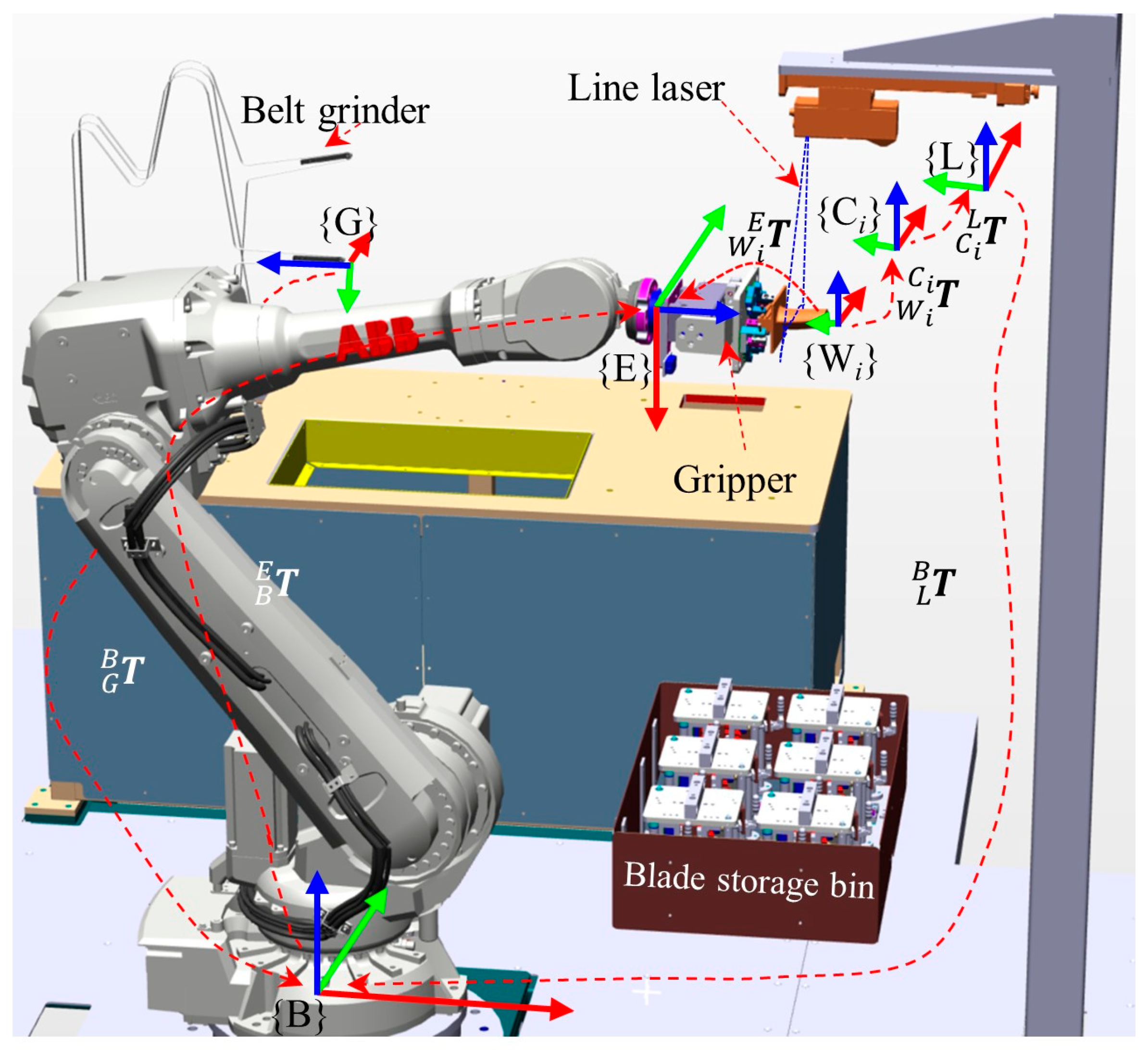
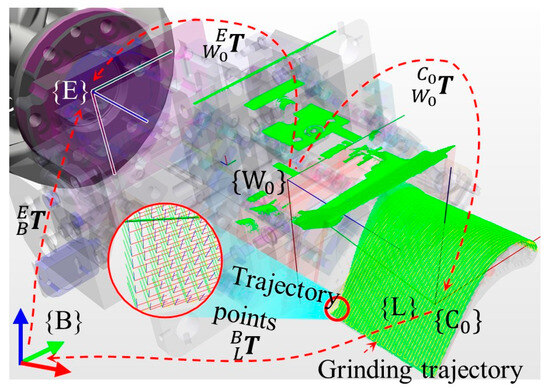
The robotic grinding system for turbine blade TBC processing is illustrated schematically in Figure 1. The system comprises five primary components. A 6-DOF articulated industrial robot that executes the grinding trajectory and handles blade-fixture transportation. A pneumatic gripper mounted on the robot end-effector for picking up blade-fixture assemblies from the storage bin. The blade storage bin contains multiple blade-fixture assemblies arranged for sequential batch processing. A line-laser scanner fixed at a scanning station in an eye-to-hand configuration, i.e., rigidly mounted with a constant spatial relationship to the robot base frame. A belt grinding or abrasive wheel station where TBC material removal is performed. The relevant coordinate frames are defined in Table 1.

Figure 1. Schematic diagram of the robotic grinding system with coordinate frame definitions.

Table 1. Coordinate frame definitions.

Frame	Symbol	Description
Robot base	{B}	World reference frame fixed to the robot mounting base
Robot end-effector	{E}	Attached to the robot mounting flange
Blade workpiece	{Wi}	Aligned with the blade CAD model origin
Line-laser scanner	{L}	Fixed to the scanning station
Point cloud	{Ci}	Captured point cloud
Grinding tool (TCP)	{G}	Tool center point of the grinding device

The homogeneous transformation from frame {A} to frame {B} is denoted ${}_A{}^B\mathit{T}$ in SE (3), and its value is expressed as ${}_A{}^B\mathit{T}=x,y,z,\mathit{rx}°,\mathit{ry}°,\mathit{rz}°$. Based on the above, the transformation matrices among the various coordinate frames in the polishing system are listed in Table 2.

Table 2. Homogeneous transformation definitions.

Transformation	Description	How to Obtain?
${}_E{}^B\mathit{T}$	Frame {E} to frame {B}	Reading from robot controller
${}_{W_i}{}^E\mathit{T}$	Frame {Wi} to frame {E}	Online updating each time
${}_L{}^{W_i}\mathit{T}$	Frame {L} to frame {Wi}	Manually calibrate very first time
${}_L{}^B\mathit{T}$	Frame {L} to frame {B}	Eye-to-hand calibration
${}_{C_i}{}^L\mathit{T}$	Frame {Ci} to frame {B}	Online calibrating by ICP
${}_G{}^B\mathit{T}$	Frame {G} to frame {B}	Manually calibrate very first time

In the turbine blade coating polishing system, the full-coverage polishing toolpath is generated on the standard CAD model or the reverse-engineered mesh model of the blade. Therefore, the toolpath points generated on the model must be mapped onto the actual blade surface in the polishing system. In essence, this requires converting the coordinate points on the blade CAD model into the robot base frame {B}. In the current system configuration, the tool coordinate frame {G} is fixed in space, while the workpiece coordinate frame moves with the end-effector {E}. Hence, given the transformation ${}_G{}^B\mathit{T}$, for each individual blade it is necessary to obtain an accurate ${}_{W_i}{}^E\mathit{T}$, and then the ABB robot control system automatically performs the coordinate transformation. According to the coordinate transformation loop {E} → {W_i} → {C_i} → {L} → {B} → {E} shown in Figure 1, the principle for computing ${}_{W_i}{}^E\mathit{T}$ is given by Equation (1):

$${}_{W_i}{}^E\mathit{T}={}_B{}^E\mathit{T}\cdot {}_L{}^B\mathit{T}\cdot {}_{C_i}{}^L\mathit{T}\cdot {}_{W_i}{}^{C_i}\mathit{T}, i\in [1,2,\dots ,n]$$

(1)

where, ${}_E{}^B\mathit{T}$ denotes the transformation from frame {E} to frame {B}, which can be directly read from the robot controller as the end-effector pose data at the scanning posture.

${}_L{}^B\mathit{T}$ denotes the transformation from frame {L} to frame {B}, which must be obtained through high-precision hand–eye calibration. ${}_{C_i}{}^L\mathit{T}$ is the transformation from the point cloud coordinate frame {C_i} to the line laser coordinate frame {L}; however, in the current application this matrix is always the identity matrix I, because the point cloud frame and the line laser frame coincide when fixturing errors are neglected. ${}_{W_i}{}^{C_i}\mathit{T}$ is the pose transformation from the blade model coordinate frame {W_i} to the point cloud frame {C_i}. In Equation (1), ${}_L{}^B\mathit{T}$ must be obtained via hand–eye calibration. By setting i = 0, the initial calibration yields ${}_{W_0}{}^{C_0}\mathit{T}$, and consequently ${}_{W_0}{}^E\mathit{T}$. This ultimately enables correct contact polishing operations under the current calibration results.

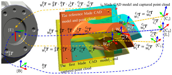
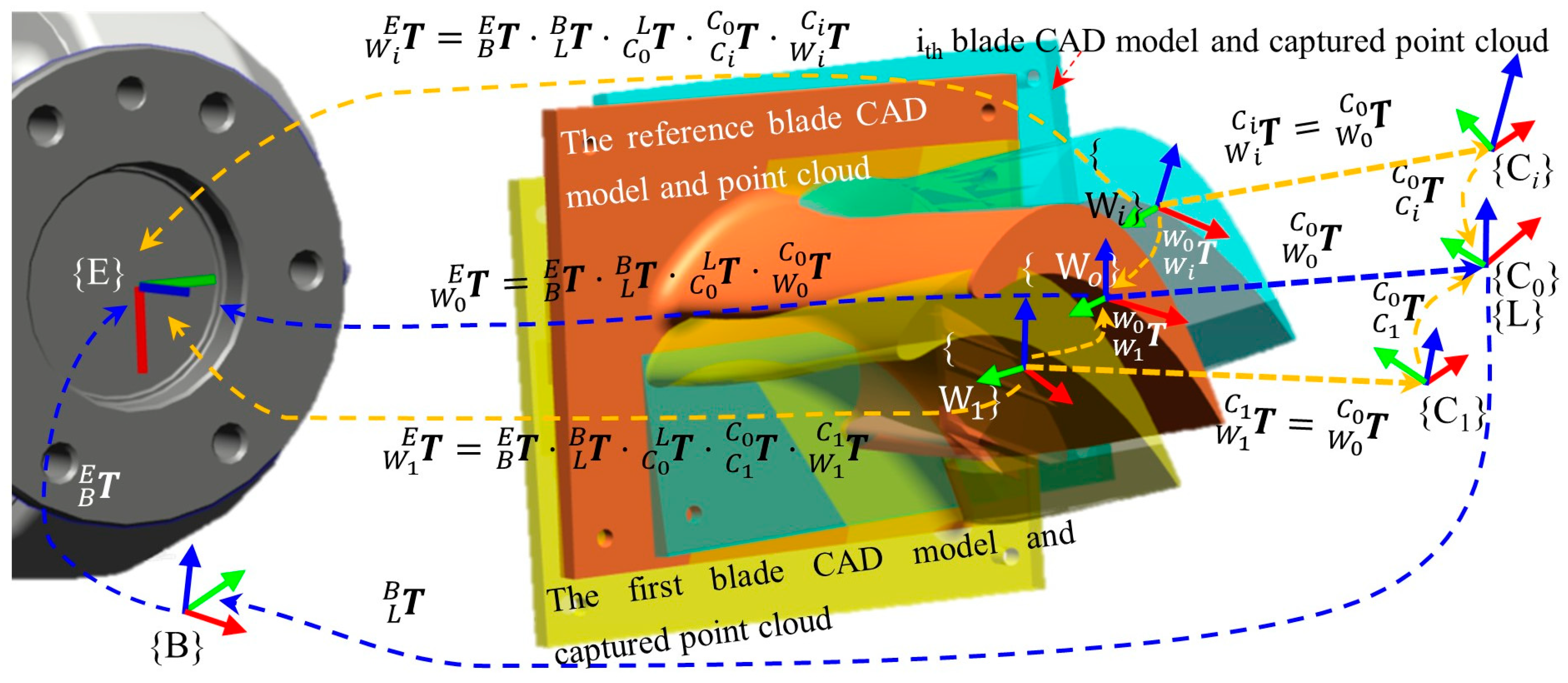
As shown in Figure 2, fixturing errors arise from long-term reuse and wear of the blade fixture. Each clamping causes slight variations in the workpiece coordinate frame ${}_{W_i}{}^E\mathit{T}$, so the calibration procedure must be re-executed to obtain updated values of ${}_{W_i}{}^{C_i}\mathit{T}$, thereby ensuring the correct workpiece frame. However, the initial calibration procedure relies on complex operational steps and advanced algorithms, requiring manual assistance to compute ${}_{W_i}{}^{C_i}\mathit{T}$, which is difficult to automate. To overcome this difficulty, a new method is proposed in this paper.

Figure 2. Schematic diagram of the robotic grinding system with clamping error.

As illustrated in Figure 2, the initially calibrated ${}_{W_0}{}^{C_0}\mathit{T}$ is taken as the reference standard. During the subsequent batch production runs (from the 1st to the i-th), it is assumed that the blade model frame {W_i} deviates from the initial pose {W₀} by a pose error ${}_{W_i}{}^{W_0}\mathit{T}$, while the scanned blade point cloud frame {C_i} simultaneously deviates from the initial point cloud frame {C₀} by a pose error ${}_{C_i}{}^{C_0}\mathit{T}$. Since the blade surface point cloud obtained by scanning represents the actual spatial pose of the blade, the model must be aligned with this point cloud so that the planned toolpath coincides with the real blade surface. Therefore, for each clamping, the pose relationship from the blade model frame {W_i} to the blade point cloud frame {C_i} always remains ${}_{W_i}{}^{C_i}\mathit{T}={}_{W_0}{}^{C_0}\mathit{T}$. Consequently, the error compensation principle shown in Figure 2 is obtained. The computation of ${}_{W_i}{}^E\mathit{T}$ can then be performed via the following three coordinate transformation loops.

(1)

Coordinate transformation loop 1: {E} → {W_i} → {C_i} → {C₀} → {L} → {B} → {E}, with the formula given by Equation (2):

$${}_{W_i}{}^E\mathit{T}={}_B{}^E\mathit{T}\cdot {}_L{}^B\mathit{T}\cdot {}_{C_0}{}^L\mathit{T}\cdot {}_{C_i}{}^{C_0}\mathit{T}\cdot {}_{W_i}{}^{C_i}\mathit{T},i\in [1,2,\dots ,n]$$

(2)

where ${}_{C_0}{}^L\mathit{T}$ is the identity matrix I, and ${}_{W_i}{}^{C_i}\mathit{T}$ = ${}_{W_0}{}^{C_0}\mathit{T}$. Thus, the only unknown is ${}_{C_i}{}^{C_0}\mathit{T}$, leading to (3):

$${}_{W_i}{}^E\mathit{T}={}_B{}^E\mathit{T}\cdot {}_L{}^B\mathit{T}\cdot {}_{C_i}{}^{C_0}\mathit{T}\cdot {}_{W_0}{}^{C_0}\mathit{T}, i\in [1,2,\dots ,n]$$

(3)

(2)

Coordinate transformation loop 2: {E} → {W_i} → {W0} → {E}, which is equivalent to coordinate transformation loop 3: {E} → {W_i} → {Ci} → {C0} → {W0} → {E}. This yields Equation (4):

$${}_{W_i}{}^E\mathit{T}={}_B{}^E\mathit{T}\cdot {}_L{}^B\mathit{T}\cdot {}_{C_i}{}^{C_0}\mathit{T}\cdot {}_{W_0}{}^{C_0}\mathit{T}, i\in [1,2,\dots ,n]$$

(4)

Loops 2 and 3 are essentially identical to loop 1. Since ${}_{W_i}{}^{C_i}\mathit{T}$ = ${}_{W_0}{}^{C_0}\mathit{T}$, we have Equation (5):

$${}_{W_i}{}^E\mathit{T}={}_{W_0}{}^E\mathit{T}\cdot {}_{W_i}{}^{W_0}\mathit{T}={}_{W_0}{}^E\mathit{T}\cdot {\left({}_{W_0}{}^{C_0}\mathit{T}\right)}^{-1}\cdot {}_{C_i}{}^{C_0}\mathit{T}\cdot {}_{W_0}{}^{C_0}\mathit{T}, i\in [1,2,\dots ,n]$$

(5)

where ${}_{W_i}{}^E\mathit{T}$ is the compensated (corrected) blade pose in {E}. Once ${}_{W_i}{}^{W_0}\mathit{T}$ is estimated, the nominal grinding trajectory, defined as a sequence of K waypoints in the blade CAD frame {W}, is remapped to the robot end-effector frame. From the above, the fixturing error ${}_{W_i}{}^{W_0}\mathit{T}$ of the blade model is computed as shown in Equation (6):

$${}_{W_i}{}^{W_0}\mathit{T}={\left({}_{W_0}{}^{C_0}\mathit{T}\right)}^{-1}\cdot {}_{C_i}{}^{C_0}\mathit{T}\cdot {}_{W_0}{}^{C_0}\mathit{T}, i\in [1,2,\dots ,n]$$

(6)

where ${}_{W_0}{}^{C_0}\mathit{T}$ is obtained from the initial calibration and serves as the reference value for subsequent grasping error compensation. For each grasping operation, ${}_{C_i}{}^{C_0}\mathit{T}$ must be computed online.

2.2. Process Workflow

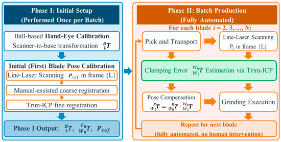
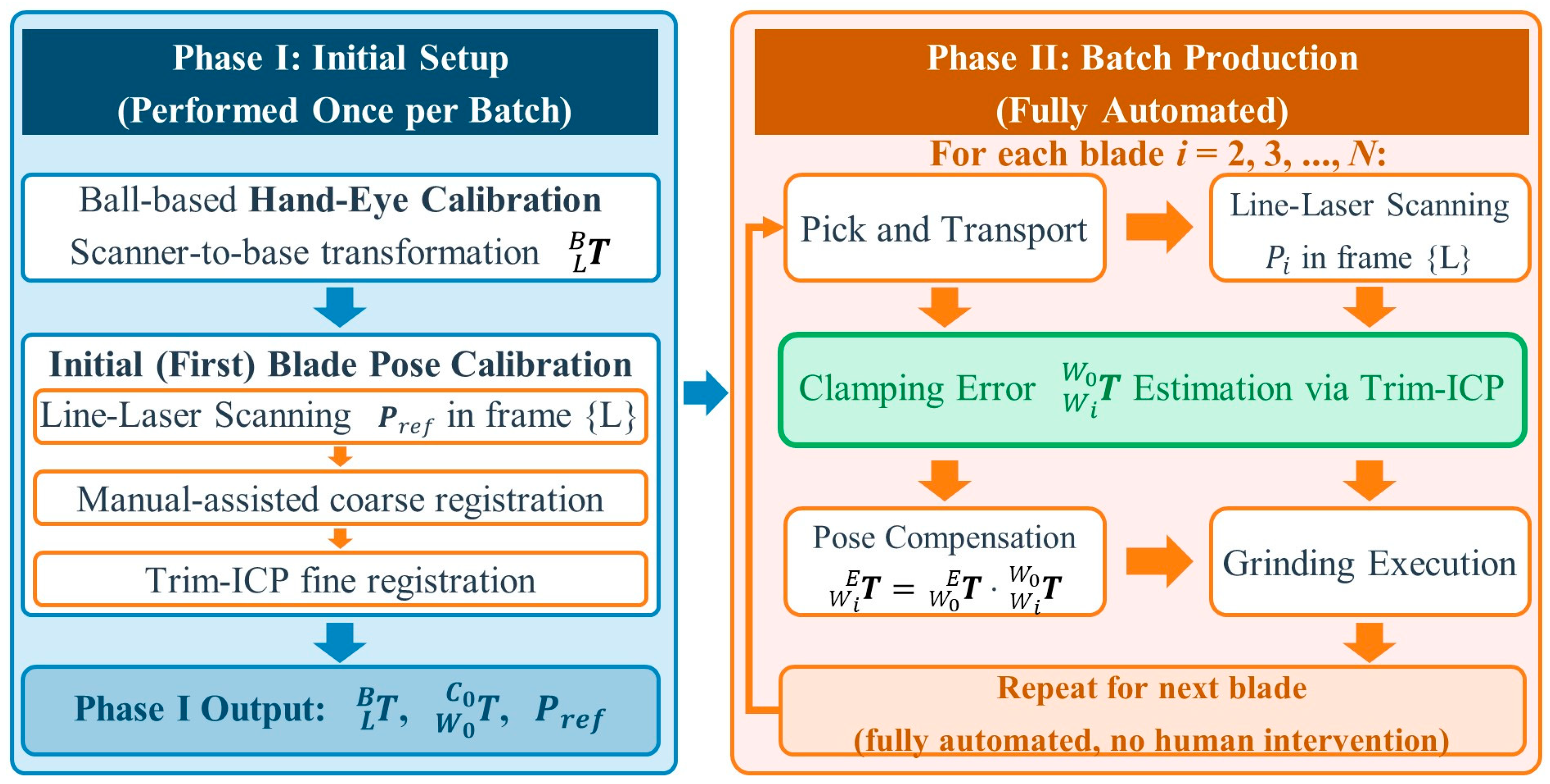
The overall workflow is divided into two phases, as depicted in Figure 3.

Figure 3. Process flow diagram showing Phase I (initial setup) and Phase II (automated batch production).

Phase I: Initial setup (performed once per batch). First, the hand–eye calibration (Section 3.3) is conducted to determine the scanner-to-base transformation ${}_L{}^B\mathit{T}$ using the ball-based method, which establishes the spatial relationship between the line-laser scanner frame {L} and the robot base frame {B}. Subsequently, the initial blade pose calibration (Section 3.4) is performed on the very first blade in the batch. The line-laser scans the blade surface, and a manual-assisted coarse registration is carried out to bring the scanned point cloud into rough alignment with the blade mesh model. This is followed by Trim-ICP fine registration to refine the alignment, yielding three essential references: ${}_{W_0}{}^{C_0}\mathit{T}$, the initial blade workpiece pose ${}_{W_0}{}^E\mathit{T}$ expressed in the robot end-effector frame {E}, and the reference point cloud P_ref captured in the scanner frame {L} or point cloud frame {C₀}. These references, once established, serve as the benchmark for all subsequent blades in the batch.

Phase II: Batch production (fully automated). For each subsequent blade I (I = 1, 2, …, N), the pneumatic gripper mounted on the robot end-effector picks the blade-fixture assembly from the bin and transports it to the fixed scanning position. The line-laser scans the blade surface, yielding the current point cloud P_i in {C_i}. At this stage, the proposed clamping error compensation method (Section 4) is invoked: since the clamping-induced pose deviation is inherently bounded by the mechanical constraints of the fixture and gripper, it lies well within the convergence basin of ICP. Consequently, fine registration via ICP between P_i and P_ref can be performed directly, without any coarse registration, to estimate the inter-blade clamping error ${}_{W_i}{}^{W_0}\mathit{T}$. The current blade pose is then compensated as ${}_{W_i}{}^E\mathit{T}={}_{W_0}{}^E\mathit{T}\cdot {}_{W_i}{}^{W_0}\mathit{T}$, and the grinding trajectory is remapped accordingly. The robot subsequently transports the blade to the grinding station and executes the compensated grinding operation. This process repeats in a fully automated loop for every blade in the batch, entirely eliminating the need for manual intervention beyond the initial calibration.

2.3. Hand-Eye Calibration

A standard-ball-based hand–eye calibration method is employed, following the approach of Li et al. [7,9]. A calibration sphere of known radius R is rigidly attached to the robot end-effector. The robot moves the sphere through M distinct poses within the scanner field of view. At each pose j (j = 1, …, M), the joint encoder readings, together with the forward kinematic model, provide the end-effector pose ${}_{E_j}{}^B\mathit{T}$. The line-laser scans the spherical surface, and least-squares sphere fitting extracts the sphere center ${}^{E}P_c$ in the scanner frame {L}. Let ${}^{E}P_c$ denote the (unknown but constant) sphere center coordinates in the end-effector frame {E}. The kinematic constraint is:

$${}_{E_j}{}^B\mathit{T}\cdot {}^{E}P_c={}_L{}^B\mathit{T}\cdot {}^{L}P_{c_j}$$

(7)

With M ≥ 3 non-collinear poses, the unknowns ${}_L{}^B\mathit{T}$ and ${}^{E}P_c$ are solved through nonlinear least-squares optimization:

$$\mathit{min}{{\sum }_j‖{}_{E_j}{}^B\mathit{T}\cdot {}^{E}P_c-{}_L{}^B\mathit{T}\cdot {}^{L}P_{c_j}‖}^2$$

(8)

The calibration quality was assessed on site by comparing the fitted sphere diameter against the nominal value and by evaluating the root-mean-square (RMS) residual of Equation (7). This calibration is performed once and remains valid as long as the scanner and robot base maintain a fixed relative pose.

2.4. Initial Blade Pose Calibration

2.4.1. Reference Point Cloud Acquisition

The first blade in the batch is picked by the gripper and presented to the line-laser scanner at the scanning station. The point cloud P_ref acquired during this initial calibration (expressed in {C₀}) is stored as the reference for all subsequent clamping error compensation operations. A critical design note: P_ref covers the entire visible region of the blade surface from the scanning station, and the same region is acquired in each subsequent scan. At the same time, the scanning pose of the end-effector needs to be stored as ${}_E{}^B\mathit{T}$.

2.4.2. Manual-Assisted Coarse Registration

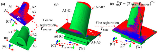
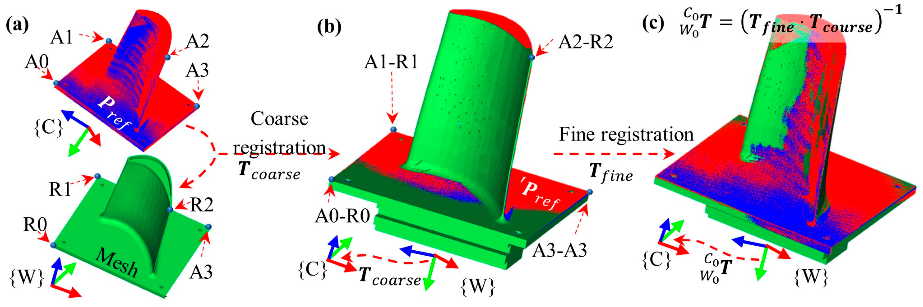
Since the blade orientation relative to the mesh model is initially unknown and may involve an arbitrary rigid transformation, a coarse registration step is required. Due to the smooth free-form nature of turbine blade airfoil surfaces, fully automatic coarse registration algorithms (SAC-IA + FPFH [14], Super4PCS [16]) are unreliable in this context: local geometric descriptors lack distinctiveness on smoothly curved surfaces, and the approximate rotational symmetry of the airfoil cross section creates ambiguities that confuse correspondence-based methods. Therefore, as shown in Figure 4a, a human operator assists by selecting K ≥ 4 corresponding point pairs on the scanned point cloud and the mesh model. A least-squares rigid transformation is then computed:

$${\mathit{T}}_{\mathit{coarse}}={\mathit{argmin}}_{\mathit{T}}{{\sum }_k‖\mathit{T}\cdot P_{\mathit{ref}}^k-P_{\mathit{mesh}}^k‖}^2$$

(9)

Figure 4. Principle and process of coarse registration and ICP-based fine registration. (a) Manually selecting corresponding point pairs; (b) coarse registration; (c) Fine registration.

The essence of this method is to minimize the sum of squared distances between all corresponding point pairs by the SVD method, thereby finding the optimal rotation and translation that best align the two point clouds in space. Then, based on the transformation T_course, the point cloud P_ref is transformed to a new pose, yielding ${}^{\prime }\mathit{P}_{\mathit{ref}}$.

2.4.3. ICP Fine Registration

The coarsely aligned point clouds are subsequently refined by fine registration to achieve the sub-millimeter accuracy required for grinding trajectory compensation. This work employs the Trimmed Iterative Closest Point (Trimmed-ICP) algorithm [30], which augments the standard ICP framework with a Least Trimmed Squares (LTS) estimator to suppress the influence of outliers, measurement noise, and partially overlapping regions inherent in line-laser scans of thin-walled turbine blade surfaces. Trimmed-ICP is an established algorithm, and it is not the contribution of this work. What is proposed here is the system-level strategy of retaining the first calibrated scan as a reference, which removes the coarse-registration step from the batch workflow.

The algorithm follows the standard ICP iterate-and-refine paradigm: given a source point cloud P_s and a target cloud Q_t, each iteration establishes nearest-neighbor correspondences, computes the residual distances, discards a fraction (1 − τ) of point pairs with the largest residuals, and estimates the rigid transformation ${\mathit{T}}_{\mathit{trim}}^{*}\in \mathit{SE}\left(3\right)$ from the retained subset via SVD-based alignment. Convergence is declared when the change in root-mean-square error falls below a prescribed threshold ϵ. A comprehensive description of the Trimmed-ICP formulation is provided in [30] by using T = TrimICP(P_s,Q_t) to describe the fine registration.

In the blade grinding workflow, Trimmed-ICP fulfills two distinct functions. During the initial blade pose calibration (Phase I, Section 3.4), as shown in Figure 4b,c, it refines the output of the manual-assisted coarse registration to determine the fine transformation T_fine (Equation (10)) and then to compute the reference transformation ${}_{W_0}{}^{C_0}\mathit{T}$ (Equation (11)) between the blade mesh model and the scanned point cloud, and simultaneously establishes the reference point cloud P_ref. During online compensation (Phase II), the same Trimmed-ICP routine directly registers each newly acquired scan from P_i to P_ref.

$${\mathit{T}}_{\mathit{fine}}=\mathit{TrimICP}({}^{\prime }\mathit{P}_{\mathit{ref}}, {\mathit{P}}_{\mathit{mesh}})$$

(10)

$${}_{W_0}{}^{C_0}\mathit{T}={\left({\mathit{T}}_{\mathit{fine}}\cdot {\mathit{T}}_{\mathit{coarse}}\right)}^{-1}$$

(11)

2.5. Online Automated Clamping Error Compensation

The core contribution of this paper is an automated clamping error compensation method that eliminates the need for manual intervention after the initial setup. The key design choice is the selection of the registration target: rather than registering each newly acquired point cloud P_i against the blade mesh model, which would require repeated coarse registration because the blade pose after a fresh pickup is unknown. This proposed method registers P_i directly against the reference point cloud P_ref to obtain the ${}_{C_i}{}^{C_0}\mathit{T}$ by following Equation (12). Because the reference point cloud and the blade mesh model must be moved from the reference position to the actual offset position, the transformation matrix returned by ICP must be inverted to obtain the required pose transformation:

$${}_{C_i}{}^{C_0}\mathit{T}={\left(\mathit{TrimICP}({\mathit{P}}_i, {\mathit{P}}_{\mathit{ref}})\right)}^{-1}$$

(12)

Then, both the compensated ${}_{W_i}{}^E\mathit{T}$ and workobject clamping error ${}_{W_i}{}^{W_0}\mathit{T}$ will be accomplished by using Equations (5) and (6), respectively. Since both P_i and P_ref are expressed in the same scanner coordinate frame {C} and are acquired by the identical sensor from the same viewing configuration, this design offers three advantages. First, no coordinate frame conversion is required, because the point clouds are directly comparable. Second, the two scans share identical noise statistics and sampling density, which improves the reliability of nearest-neighbor correspondence within ICP. Third, the initial misalignment between P_i and P_ref is solely attributable to the clamping error, which is strictly bounded by the mechanical constraints of the gripper and fixturing system.

The clamping error ${}_{W_i}{}^{W_0}\mathit{T}$ is decomposed into a rotation ${}_{W_i}{}^{W_0}\mathit{R}\in \mathit{SO}(3)$ and a translation ${}_{W_i}{}^{W_0}\mathit{t}\in {\mathbb{R}}^3$. The magnitude of the clamping deviation is governed by the repeatability of the pneumatic gripper and by the clearances and flatness tolerances of the fixture locating surfaces. It is not a fixed quantity: it differs between fixtures and grows as those surfaces wear, so no single bound can be assumed. The proposed method therefore does not rely on an assumed magnitude; the deviation is measured on every pickup by registering the current scan against the reference, and requires only that the deviation be bounded, so that it lies within the convergence basin of ICP. The recorded maximum remains inside this basin, which extends to rotational misalignments of approximately 30° and to translational offsets of the order of the correspondence search radius [20,23]. Consequently, the identity matrix I serves as a valid initialization for the ICP optimization, and coarse registration is unnecessary. Convergence of the solver is a necessary but not sufficient condition for a correct result, and the possibility of convergence to a spurious local minimum requires consideration. Three features of the proposed workflow limit this risk. First, the optimization is always initialized from the identity transformation, and the displacement it must recover is bounded by the mechanical design of the gripper and fixture. Second, both clouds are acquired by the same sensor from the same viewpoint, so the point-to-point correspondence at the correct solution is near-ideal, which further reduces the likelihood of trapping in a spurious minimum. Third, results are not accepted on the strength of the convergence flag alone: each is screened for physical plausibility, and displacements exceeding 10 mm or 5° are rejected as misregistrations.

3. Experiment and Results

3.1. Experimental Platform and Procedure

The experimental platform is shown in Figure 1 and comprises the following components: a 6-DOF industrial robot (ABB Engineering (Shanghai) Ltd, Shanghai, China; model IRB4600, rated payload 60 kg, positioning repeatability ±0.06 mm) equipped with a pneumatic gripper on the end-effector; a line-laser profilometer (LMI Technologies Inc., Burnaby, BC, Canada; model Gocator, depth resolution 13 μm) mounted at a fixed scanning station in an eye-to-hand configuration; a belt grinding station with an abrasive belt; and a dedicated blade-fixture system. The line-laser scanner is rigidly mounted relative to the robot base, and their relative pose remains unchanged throughout all experiments. The robot controller communicates with the host computer via ProfiNet, which coordinates the scanning, registration, and trajectory remapping pipeline.

Four types of turbine blades, designated T1, T2, T3, and T4, were used in the experiments. They span a twofold range of characteristic radius, from 100 mm to 200 mm, and their reference scans contain between 1.26 × 10⁵ and 1.82 × 10⁵ points (Table 3), so they differ appreciably in developed area and curvature. The chord, span, and thickness distributions are withheld, as the blades are customer components supplied under confidentiality. The reference blade models were created by reverse engineering, and each blade is mounted on a dedicated fixture that interfaces with the pneumatic gripper. Throughout, dimensional quantities are given in millimeters and coating thickness and roughness in micrometers.

Table 3. Experimental dataset summary.

Blade Type	Number of Trials	Time Period	Characteristic Radius r (mm)	Reference Scan (×103)
T1	140	February 2025–January 2026	150	126.0
T2	125	February 2025–January 2026	200	163.6
T3	145	February 2025–January 2026	100	134.9
T4	120	December 2024–January 2025	160	182.2

Notes: the time periods are derived from the acquisition timestamps of the scan files of each blade type.

Experimental procedure. The experiments were conducted in two phases following the workflow described in Section 3.2:

Phase I—Initial setup. (1) The hand–eye calibration was performed using the ball-based method (Section 3.3) with a standard calibration sphere (diameter 25 mm, Grade 0.001). The robot moved the sphere through M = 10 distinct poses within the scanner’s field of view, and the transformation ${}_L{}^B\mathit{T}$ was estimated via nonlinear least-squares optimization. (2) For each of the four blade types, the initial blade pose calibration (Section 3.4) was performed: the first blade was picked, scanned by the line-laser, and manually co-registered to its mesh model by selecting corresponding point pairs, followed by ICP fine registration. The resulting reference blade pose ${}_{W_0}{}^{C_0}\mathit{T}$, ${}_{W_0}{}^E\mathit{T}$ and the reference point cloud P_ref were stored as permanent references for that blade type.

Phase II—Automated batch production validation. To validate the proposed clamping error compensation method under realistic production conditions, each blade type was repeatedly picked, scanned, and compensated over an extended period. For each pickup trial, the robot transported the blade to the scanning station, the line-laser acquired the current point cloud P_i, and the ICP registration against P_ref was executed to estimate the clamping error ${}_{W_i}{}^{W_0}\mathit{T}$. The compensated workpiece pose was computed via Equation (5) and the grinding trajectory was remapped accordingly. A total of 538 pickup records were collected; eight were rejected by the plausibility screen of Section 3, and the remaining 530 valid trials are analysed in Table 3.

3.2. Hand-Eye Calibration Validation

The hand–eye calibration was performed using 10 sphere poses. The fitted sphere center positions in the line-laser frame {L} were paired with the corresponding end-effector poses {E} read from the robot controller, and the transformation ${}_L{}^B\mathit{T}$ was solved via the nonlinear least-squares formulation given in Equation (8). The sphere-fit residual of Equation (7) and the reconstructed sphere diameter were used to accept the calibration on site, but only the resulting transformation was retained: the underlying measurements were not archived, and the cell has since been handed over, so neither value can be reported retrospectively. The calibration is therefore documented below by a loop-closure consistency check, which verifies the internal coherence of the chain, and by the end-to-end process results. The calibration yielded the result ${}_L{}^B\mathit{T}$ = 1027.43, 0.46, 1624.81, 0.11°, 0.17°, and 89.37°. The calibration was performed once, and its validity was verified periodically. Over the 12-month experimental campaign, no detectable drift was observed, confirming the long-term stability of the fixed eye-to-hand configuration.

3.3. Initial Blade Pose Calibration

The initial blade pose calibration was executed once per blade type to establish ${}_{W_0}{}^E\mathit{T}$ and P_ref. For each blade type, the procedure involved the following steps.

3.3.1. Coarse Registration

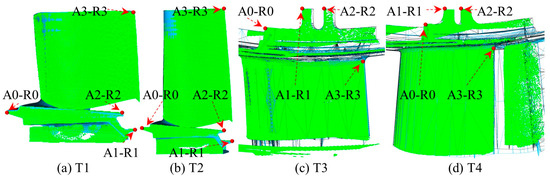
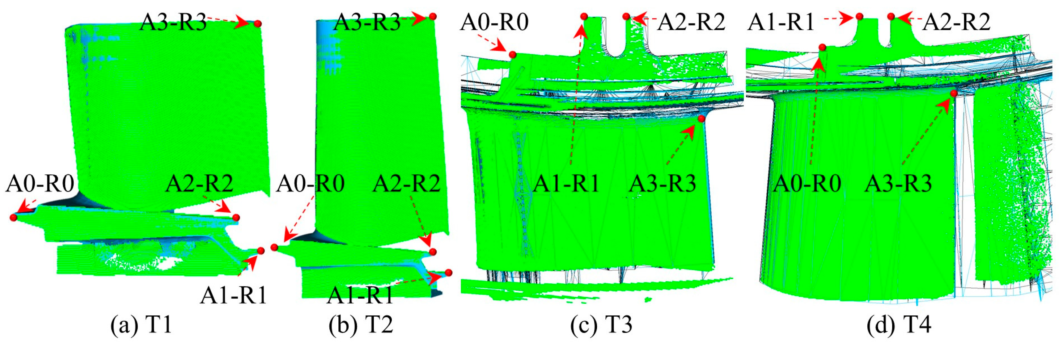
An operator manually selected K = 4 corresponding point pairs on the scanned point cloud and the mesh model. The pairs were chosen at geometrically distinctive locations such as the blade platform edges, the leading and trailing edge extremities, and the root-fixture interface. A least-squares rigid transformation was computed from these correspondences, yielding the coarse alignment T_coarse. The results of each blade were shown in Table 4 and Figure 5, respectively.

Table 4. Manual point pairs for coarse registration and the resulting transformations.

Blade Type		Points in Pref		Points in Mesh Model	Coarse Registration RMSE (mm)	Tcoarse
T1	A0	56.20, 45.32, 61.25	R0	−31.70, 69.52, 76.01	0.7811	32.2220, 10.3300, 112.6680 −81.9676°, 0.7605°, 87.1057°
	A1	53.20, 60.00, 51.42	R1	−30.18, −40.55, 60.93
	A2	−43.00, 46.33, 55.14	R2	−31.34, −30.30, 74.25
	A3	−50.40, −46.84, 13.40	R3	23.50, −38.72, 162.47
T2	A0	−32.38, 63.82, 74.00	R0	−32.15, 64.20, 74.76	0.6652	36.7542, 14.2436, 114.8393 −83.4331°, 0.9410°, 92.6630°
	A1	−30.49, −42.87, 58.77	R1	−30.65, −43.52, 58.31
	A2	−31.95, −33.13, 70.45	R2	−31.97, −33.35, 70.21
	A3	18.537, −32.64, 213.52	R3	18.48, −32.15, 213.45
T3	A0	−31.03, 6.22, −17.77	R0	−31.47,5.67, −17.54	0.5856	−3.9560, 14.1665, 4.8269 95.1245°, 0.2331°, −82.8327°
	A1	−13.06, 35.36, −35.06	R1	−13.13, 35.11, −35.05
	A2	−8.00, 40.42, −35.04	R2	−7.64, 40.76, −35.41
	A3	0.46, 48.55, −35.69	R3	0.27, 48.55, −36.05
T4	A0	−21.26, 19.27, −22.45	R0	−21.43, 19.02, −22.61	0.4080	16.4279, 2.8468, 37.1370 92.2429°, −4.2454°, −135.0266°
	A1	1.21, 24.31, −38.65	R1	1.41, 24.77, −38.68
	A2	22.04, 25.14, −40.25	R2	21.87, 24.88, −39.87
	A3	51.05 40.64, −2.58	R3	51.18, 40.69, −2.76

Figure 5. Alignment of the reference point cloud with the blade mesh model after coarse registration.

3.3.2. Fine Registration

Using T_coarse as the initial estimate and transforming the P_ref, Trim-ICP was executed to refine the alignment according to Equation (10). T_fine will be output. The deployed implementation is characterized by the parameters listed in Table 5. Two parameters that share the numerical value 0.90 are distinct and should not be conflated: the trimming ratio τ = 0.90, which determines the fraction of correspondences retained in the LTS step, and the new-to-old energy ratio of 0.90, which is the internal stopping criterion of the solver. The transformation epsilon of the solver is a separate parameter and is not set to 0.90.

Table 5. Deployed registration parameters.

Parameter	Value	Parameter	Value
Initial transformation	Identity matrix I	Plane segmentation	points with signed distance > 5.0 mm from the fixture cut plane retained
Trimming ratio τ	0.90	Voxel downsampling	1.2 × 1.2 × 1.2 mm
Correspondence search	nearest neighbour by KD-tree	Raw scan size	1.3 × 105–1.9 × 105 points
Solver stopping criterion	new-to-old energy ratio 0.90	Solver inner iterations	terminated by the energy-ratio criterion
Outer repeat count	300	After segmentation and downsampling	≈5 × 104 points
Software	PCL 1.8.1; Visual Studio 2022	Hardware	Intel Core i7-10700, 16 GB RAM; CPU only, no GPU

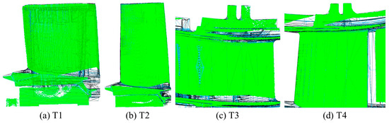
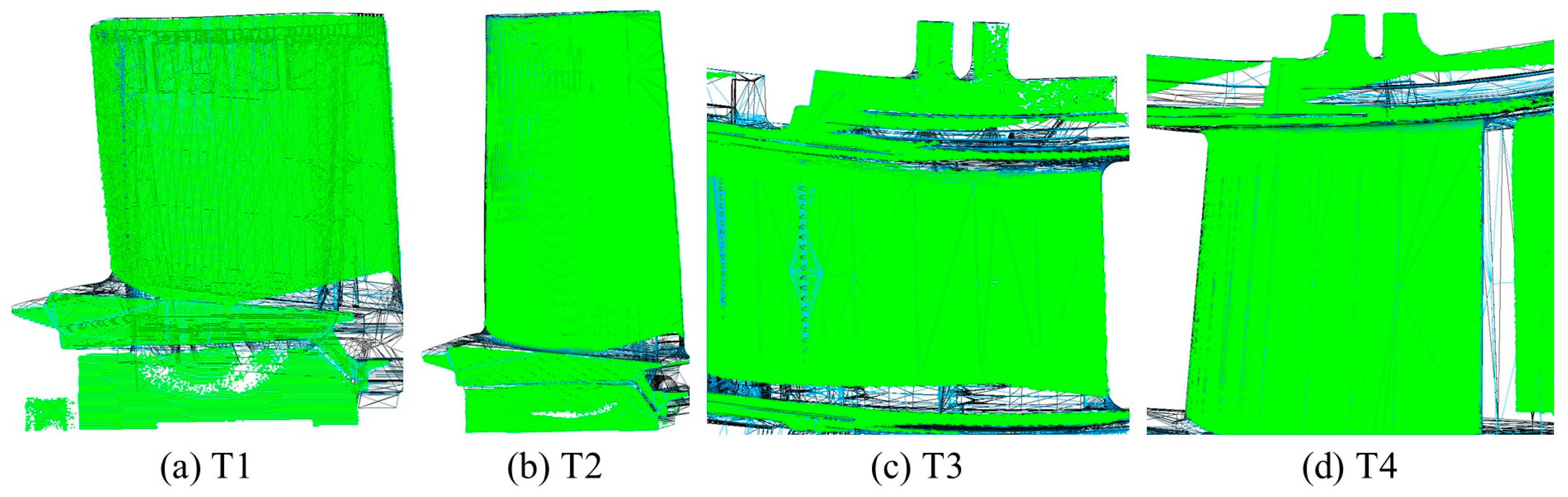
The final registration result ${}_{W_0}{}^{C_0}\mathit{T}$ (referring to Equation (11)) was stored together with the reference point cloud P_ref. The results of each blade were shown in Table 6 and Figure 6, respectively.

Table 6. Initial blade pose calibration results after Trimmed-ICP fine registration.

Blade Type	ICP Fitness Score	Tfine	${}_{{\mathit{W}}_0}{}^{{\mathit{C}}_0}\mathit{T}={\left({\mathit{T}}_{\mathit{fine}}\cdot {\mathit{T}}_{\mathit{coarse}}\right)}^{-1}$	${}_{{\mathit{W}}_0}{}^{\mathit{E}}\mathit{T}={}_{\mathit{B}}{}^{\mathit{E}}\mathit{T}\cdot {}_{\mathit{L}}{}^{\mathit{B}}\mathit{T}\cdot {}_{{\mathit{C}}_0}{}^{\mathit{L}}\mathit{T}\cdot {}_{{\mathit{W}}_0}{}^{{\mathit{C}}_0}\mathit{T}$
T1	0.2468	0.5602, 0.2905, −0.0990 0.0056°, 0.0202°, 0.2170°	−10.7822, 116.1317, 16.0352 19.0834°, 81.1772°, −71.2116°	−10.7822, 116.1317, 16.0352 19.0834°, 81.1772°, −71.2116°
T2	0.2108	1.2443, −0.4509, −0.8133 0.2280°, −0.0000°, 0.4959°	−10.1308, 117.8742, 25.2768 24.0731°, 84.2151°, −115.8532°	−10.1308, 117.8742, 25.2768 24.0731°, 84.2151°, −115.8532°
T3	0.1435	−0.0401, 0.1230, 0.3487 0.4090°, 0.0803°, 0.2191°	14.6950, −5.2912, −1.7166 124.1511°, 81.0798°, −33.9913°	14.6950, −5.2912, −1.7166 124.1511°, 81.0798°, −33.9913°
T4	0.1490	−0.7841, −0.0758, 0.2317 0.2450°, 0.1490°, −0.1130°	10.2214, −37.8425, 10.5870 93.2586°, 44.9915°, 177.7775°	10.2214, −37.8425, 10.5870 93.2586°, 44.9915°, 177.7775°

Figure 6. Alignment of the reference point cloud with the blade mesh model after fine registration.

3.3.3. Calibration Quality Verification

Since no external metrology equipment (e.g., CMM, photogrammetry, or laser tracker) was available in the industrial cell, the initial calibration quality was verified through the following internal consistency checks:

(1)

Registration fitness score. The RMS point-to-point distance between the aligned point cloud and the mesh model at ICP convergence was 0.2468 mm for T1, 0.2108 mm for T2, 0.1435 mm for T3, and 0.1490 mm for T4, indicating that the two clouds agree to the sub-millimeter level across all blade types, as shown in Table 6.

(2)

Visual inspection. The aligned point cloud was overlaid on the mesh model and visually inspected to ensure that the airfoil curvature, platform geometry, and root features were correctly aligned without systematic offsets; see Figure 6 for a representative registration result.

(3)

Hand-eye consistency verification. To assess the consistency of the calibration chain and kinematic consistency of the hand–eye transformation ${}_L{}^B\mathit{T}$, this matrix was re-derived from the calibration data of four different blades using the coordinate loop closure constraint, as shown in Figure 7. Because several quantities inside the loop were themselves obtained from the calibration, the test establishes the consistency of the chain rather than an independent measure of accuracy. The verification follows the closed-loop principle: first, the workpiece coordinate frame is constructed via the forward kinematics equation ${}_{W_0}{}^E\mathit{T}={}_B{}^E\mathit{T}\cdot {}_L{}^B\mathit{T}\cdot {}_{C_0}{}^L\mathit{T}\cdot {}_{W_0}{}^{C_0}\mathit{T}$; then, the hand–eye transformation is inversely recovered using ${}_L{}^B\mathit{T}={}_E{}^B\mathit{T}\cdot {}_{W_0}{}^E\mathit{T}\cdot {}_{C_0}{}^{W_0}\mathit{T}\cdot {}_L{}^{C_0}\mathit{T}$. The four (T1, T2, T3, T4) recomputed results were compared element-wise with the calibration reference ${}_L{}^B\mathit{T}$.

Figure 7. Coordinate loop closure verification of the hand–eye transformation.

As shown in Table 7, statistical analysis shows that the maximum comprehensive translational deviation (Euclidean distance) is 0.0323 mm, the maximum rotational vector deviation is 0.0057°, and the average comprehensive translational deviation is only 0.0144 mm. This confirms that even when different blades are measured with re-clamping errors, the system maintains highly stable coordinate solutions, thereby verifying the kinematic consistency of the entire calibration chain and the good generalization performance of the hand–eye parameters.

Table 7. Loop-closure consistency verification of the hand–eye transformation.

Blade Type	${}_{\mathit{L}}{}^{\mathit{B}}\mathit{T}={}_{\mathit{E}}{}^{\mathit{B}}\mathit{T}\cdot {}_{{\mathit{W}}_0}{}^{\mathit{E}}\mathit{T}\cdot {}_{{\mathit{C}}_0}{}^{{\mathit{W}}_0}\mathit{T}\cdot {}_{\mathit{L}}{}^{{\mathit{C}}_0}\mathit{T}$	Pose Deviation (vs. Reference)	Overall Translation Error (mm)
T1	1027.4304, 0.4477, 1624.7973, 0.1101°, 0.1730°, 89.3735°	0.0008, 0.0090, 0.0107, 0.0016°, 0.0012°, 0.0014°	0.0140
T2	1027.4291, 0.4491, 1624.8084, 0.1093°, 0.1712°, 89.3741°	0.0005, 0.0076, 0.0004, 0.0008°, 0.0006°, 0.0008°	0.0076
T3	1027.4297, 0.4877, 1624.8170, 0.1074°, 0.1692°, 89.3806°	0.0001, 0.0310, 0.0090, 0.0011°, 0.0026°, 0.0057°	0.0323
T4	1027.4295, 0.4531, 1624.8086, 0.1090°, 0.1717°, 89.3744°	0.0001, 0.0036, 0.0006, 0.0005°, 0.0001°, 0.0005°	0.0037
Max.		0.0008, 0.0310, 0.0107, 0.0016°, 0.0026°, 0.0057°	0.0323

Table note: Calibrated Hand-Eye Pose ${}_L{}^B\mathit{T}$ = 1027.4296, 0.4567, 1624.8080, 0.1085°, 0.1718°, 89.3749°. The overall translation error is $\sqrt{\Delta x^2+\Delta y^2+\Delta z^2}.$

The registration strategies were compared on identical, identically preprocessed inputs (Table 8). With identity initialization, which corresponds to the compensation case, the deployed Trimmed-ICP succeeded on all four blade types, whereas standard ICP, point-to-plane ICP, GICP, and LM-ICP succeeded on three, two, two, and three of the four, at lower computation cost. Both feature-based coarse methods failed on every blade type and on every large-offset case and required one to two orders of magnitude more computation time, which is the practical reason why the reference-scan strategy avoids coarse registration altogether.

Table 8. Comparison of registration strategies on identically preprocessed cloud pairs.

Method	Agreement with the Deployed Result	Mean Residual (mm)	Mean Time (s)
Trimmed-ICP (deployed)	4/4	0.452	8.6
ICP	3/4	0.450	1.4
Point-to-plane ICP	2/4	0.458	0.6
GICP	2/4	0.478	0.8
LM-ICP	3/4	0.454	2.0
SAC-IA + FPFH	0/4	2.051	328
SCP + FPFH	0/4	1.123	96

Notes: agreement denotes reproduction of the deployed result within 0.5 mm and 0.5°; the Trimmed-ICP row is the reference. Times are comparable between methods. For applied offsets of 15–45°, Trimmed-ICP recovered the offset in 1 of 12 cases and in none of the others. Super4PCS was not tested: not part of the on-cell library.

3.4. Clamping Error Compensation Validation

3.4.1. Quantifying the Clamping Error Magnitude

The clamping error $∆{\mathit{T}}_i={}_{W_i}{}^{W_0}\mathit{T}\in \mathit{SE}\left(3\right)$ is a rigid-body transformation comprising a translational component ∆t_i ∈ ℝ³ and a rotational component ∆R_i ∈ SO(3). To characterize the severity of the clamping error across multiple pickups, both components must be evaluated quantitatively.

(1)

Translation error. The norm of the translational deviation provides a scalar summary of the positioning error:

$$‖∆{\mathit{t}}_i‖=\sqrt{t_x^2+t_y^2+t_z^2}$$

(13)

This quantity, denoted e_uncomp in the subsequent error analysis, represents the Euclidean distance between the reference workpiece origin and the actual workpiece origin. The per-axis components t_x, t_y, and t_z further reveal directional bias: for instance, a noticeably larger standard deviation along the gripper approach direction may indicate jaw clearance asymmetry, providing actionable information for fixture maintenance.

(2)

Rotation error. From the rotation matrix ∆R_i, the total angular deviation θ(∆R_i) is extracted via the axis-angle relationship:

$$\theta (∆{\mathit{R}}_i)=\arccos \left({\displaystyle \frac{\mathrm{tr}\left(∆{\mathit{R}}_i\right)-1}{2}}\right)$$

(14)

where tr(⋅) denotes the matrix trace. The quantity θ(∆R_i) represents the magnitude of rotation about the equivalent axis and is independent of the axis direction. The per-axis Euler angles r_x, r_y, r_z extracted from ∆R_i complement this scalar metric by resolving the rotation into physically meaningful components aligned with the robot end-effector axes.

(3)

Practical significance for grinding. While ‖∆t_i‖ (e_uncomp) and θ(∆R_i) characterize the error at the workpiece coordinate origin, the trajectory error at a surface point p on the blade has an additional rotational contribution. For a point at radial distance r = ‖p‖ (Table 3) from the workpiece origin, the rotation θ induces a tangential displacement of approximately rsinθ. This amplification effect is particularly significant for large turbine blades: a seemingly modest angular error of 1° produces a tip displacement exceeding 2.6 mm for a blade with a characteristic radius of 150 mm. Therefore, both the translational and rotational components of the clamping error must be monitored and compensated to ensure uniform coating removal across the entire blade surface.

Because no external metrology was available, the registration estimate was additionally verified against a known ground truth: the reference cloud was displaced by a program-generated rigid transformation and registered back onto the unperturbed reference. Because the perturbation is generated by the test program, it never passes through the registration, and the comparison therefore provides an independent measure of the estimation error. Over sweeps of 0.5–15 mm and 0.5–10° along and about each scanner axis on all four types, the estimate reproduced the applied perturbation to within 0.5 mm and 0.5° throughout for translations within the scan plane and rotations about the blade stacking axis, and over a narrower range along the fixture plane normal.

3.4.2. Qualitative Assessment of Compensation Effectiveness

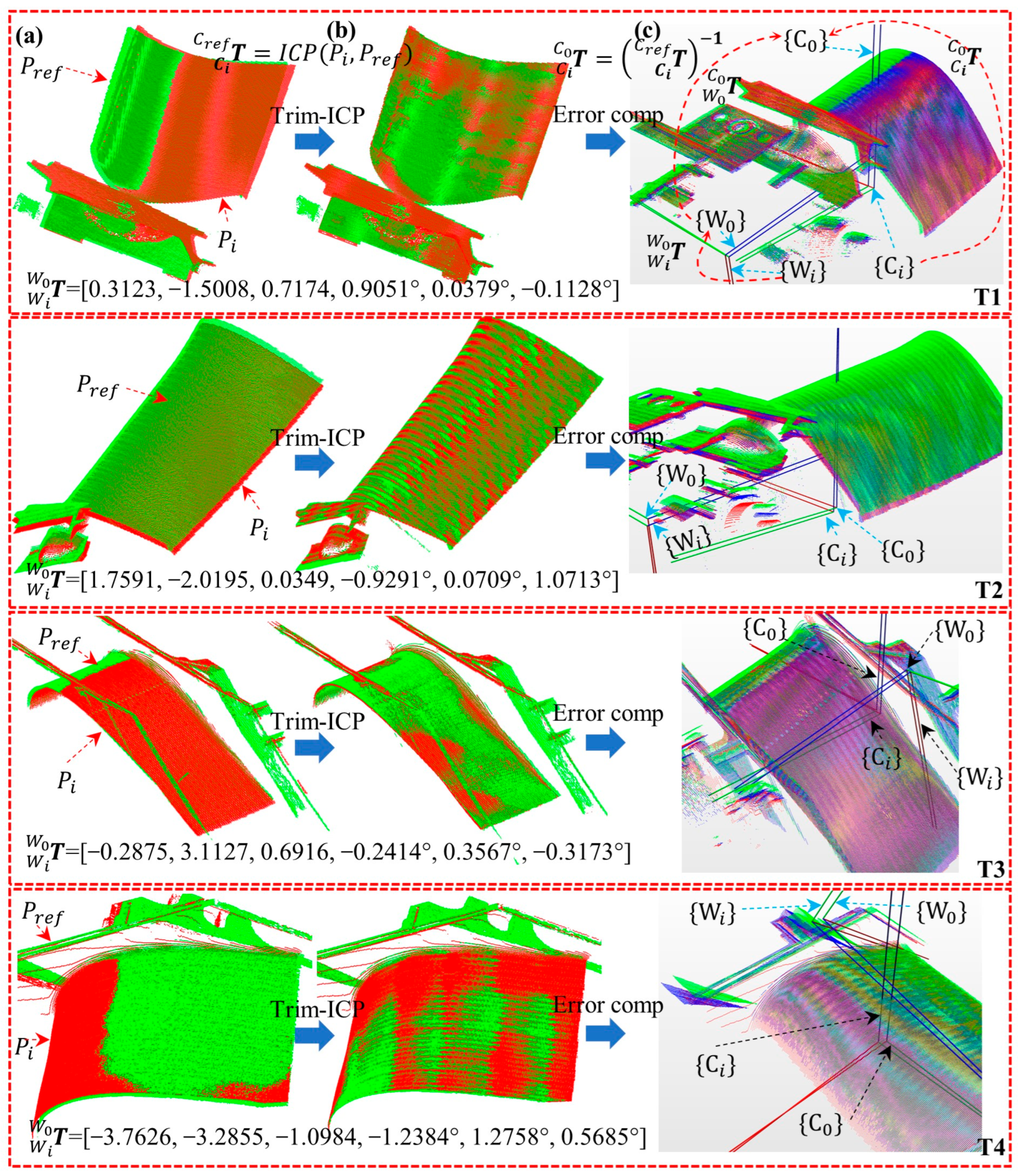
To visually assess the effectiveness of the proposed compensation, Figure 8 presents representative point cloud registration results before and after error compensation for all four blade types. Each subfigure contains three overlay views: (a) The reference point cloud P_ref (displayed in green) and the current scan P_i before compensation (displayed in red), illustrating the initial misalignment caused by the clamping error; (b) P_ref and the compensated point cloud ${\mathit{P}}_{\mathit{comp}}={}_{C_i}{}^{C_0}\mathit{T}\cdot {\mathit{P}}_i$, demonstrating the alignment after ICP registration; and (c) the corresponding workpiece coordinate systems {W₀} and {W_i} before and after compensation, showing the corrective rigid-body transformation.

Figure 8. Qualitative comparison of point cloud registration before and after clamping error compensation for four blade types. For each type, the left panel (a) shows the uncompensated overlay P_ref vs. P_i, the center panel (b) shows the compensated overlay, and the right panel (c) shows the error between workpiece coordinate frame {W} and point cloud frame {C}.

Across all four blade types, the uncompensated point clouds exhibit noticeable translational and rotational offsets relative to the reference P_ref, particularly visible at the blade tip and leading/trailing edge regions where geometric curvature is highest. After applying the proposed compensation, the two pointclouds overlap to within the sensor noise level, confirming that the Trim-ICP registration accurately recovers the clamping error. The residual misalignment is uniform and on the order of the ICP fitness score ε_fit, with no visible systematic bias.

The workpiece coordinate system visualization further reveals that the clamping error is dominated by translation along the gripper approach direction (as shown in Figure 8c). The compensation effectively realigns the workpiece frame to its reference pose, providing a correct basis for subsequent trajectory remapping.

3.4.3. Quantitative Analysis of Compensation

This section presents a comprehensive quantitative evaluation of the clamping error compensation method across the 530 experimental trials, structured along five analysis dimensions.

(1)

Point cloud displacement ${}_{C_i}{}^{C_0}\mathit{T}$ and workpiece clamping error ${}_{W_i}{}^{W_0}\mathit{T}$. The transformation ${}_{C_i}{}^{C_0}\mathit{T}$ represents the rigid-body displacement between the reference point cloud and the current scan, directly output by the Trim-ICP fine registration. According to Equation (6), ${}_{W_i}{}^{W_0}\mathit{T}$ is related to ${}_{C_i}{}^{C_0}\mathit{T}$ through a similarity transform by ${}_{{\mathrm{W}}_0}{}^{C_0}\mathit{T}$. The point cloud displacement ${}_{C_i}{}^{C_0}\mathit{T}$ is transformed into the workpiece clamping error ${}_{W_i}{}^{W_0}\mathit{T}$ expressed in the blade frame. Table 9 summarizes the translational and rotational components of ${}_{C_i}{}^{C_0}\mathit{T}$, ${}_{W_i}{}^{W_0}\mathit{T}$, and ${‖∆{\mathit{t}}_i‖}_W$/${‖∆{\mathit{t}}_i‖}_C$ across all valid trials. The translational displacement of ${}_{C_i}{}^{C_0}\mathit{T}$ ranges from 1.30 to 3.38 mm, and the rotational displacement from 0.66° to 0.90°. These values are consistent with the mechanical tolerance analysis of the pneumatic gripper and blade-fixture system and remain well within the convergence basin of ICP.

Table 9. Point cloud displacement ${}_{C_i}{}^{C_0}\mathit{T}$ statistics.

Blade Type	N	${‖∆{\mathit{t}}_{\mathit{i}}‖}_{\mathit{C}}$ Mean (mm)	${‖∆{\mathit{t}}_{\mathit{i}}‖}_{\mathit{C}}$ Max (mm)	${‖∆{\mathit{t}}_{\mathit{i}}‖}_{\mathit{W}}$ Mean (mm)	${‖∆{\mathit{t}}_{\mathit{i}}‖}_{\mathit{W}}$ Max (mm)	θ(∆Ri) Mean (°)	θ(∆Ri) Max (°)	${‖∆{\mathit{t}}_{\mathit{i}}‖}_{\mathit{W}}$/${‖∆{\mathit{t}}_{\mathit{i}}‖}_{\mathit{C}}$ Mean ± SD
T1	140	3.38	9.61	2.0316	8.3296	0.90	1.41	0.54 ± 0.17
T2	125	2.02	8.23	1.3582	8.1424	0.84	2.13	0.61 ± 0.27
T3	145	1.30	4.06	1.3682	4.1338	0.66	1.98	1.07 ± 0.07
T4	120	1.89	4.84	2.1564	6.0138	0.72	1.97	1.15 ± 0.19

(2)

Comparison between ${}_{C_i}{}^{C_0}\mathit{T}$ and ${}_{W_i}{}^{W_0}\mathit{T}$. The translational norms differ systematically depending on the blade type. A comparison of ${‖∆{\mathit{t}}_i‖}_W$ and ${‖∆{\mathit{t}}_i‖}_C$ reveals an important geometric distinction. As shown in Table 9, the ratio $‖{}_{W_i}{}^{W_0}\mathit{t}‖/‖{}_{C_i}{}^{C_0}\mathit{t}‖$ was computed for each trial. The overall mean ratio across all 530 valid trials was 0.84 ± 0.33. For T3 and T4 blades, the ratio was close to or slightly above unity (1.07 ± 0.07 and 1.15 ± 0.19, respectively), indicating that the workpiece frame origin is located close to the point-cloud centroid and thus the rotational contribution to the translational error is negligible. In contrast, for the blade T1 and T2, ${‖∆{\mathit{t}}_i‖}_W$ is systematically smaller than ${‖∆{\mathit{t}}_i‖}_C$ (mean ratio 0.54 for T1 and 0.61 for T2). This reduction arises because the workpiece coordinate origin is offset from the blade centroid, and the rotational component of the clamping error partially cancels the translational displacement in the workpiece frame. The rotational components of ${}_{W_i}{}^{W_0}\mathit{T}$ and ${}_{C_i}{}^{C_0}\mathit{T}$ are verified to be identical across all trials (|θ_W − θ_C| ≤ 10⁻⁶), confirming that the rotation angle is invariant under the similarity transform of Equation (6), while the translational component is modulated by the lever-arm distance between the two reference points. These observations highlight that reporting only the point-cloud registration error ${‖∆{\mathit{t}}_i‖}_C$ may overestimate or underestimate the actual trajectory error at the grinding surface, depending on the geometric configuration; the workpiece-frame error ${‖∆{\mathit{t}}_i‖}_W$ is the physically relevant quantity for trajectory compensation.

(3)

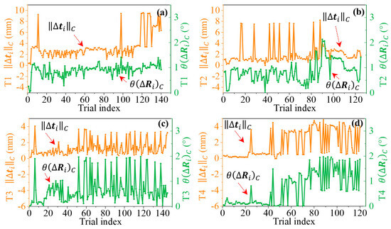
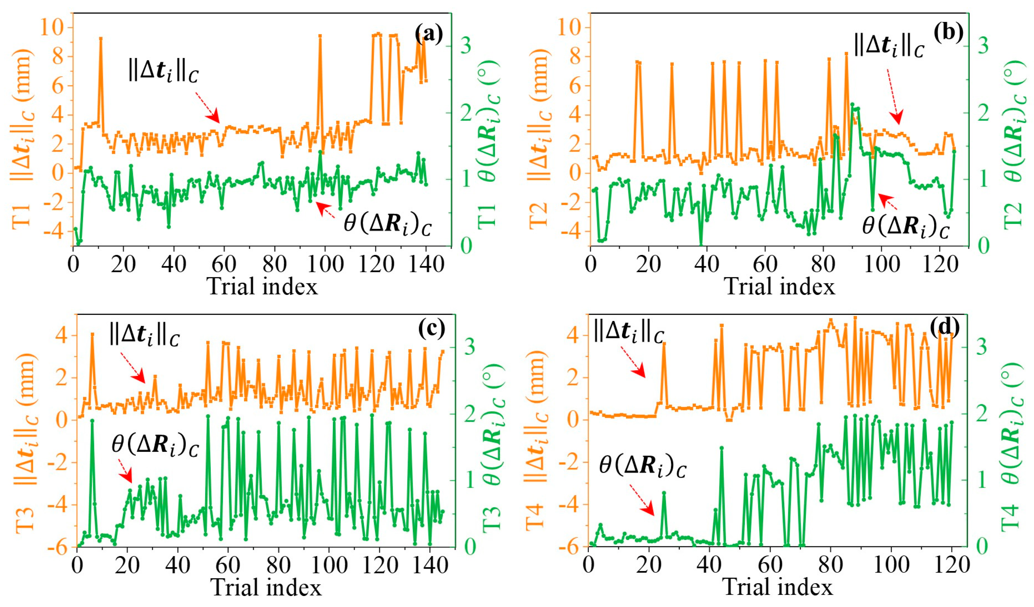
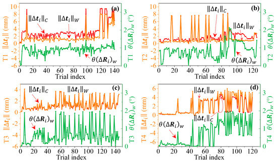
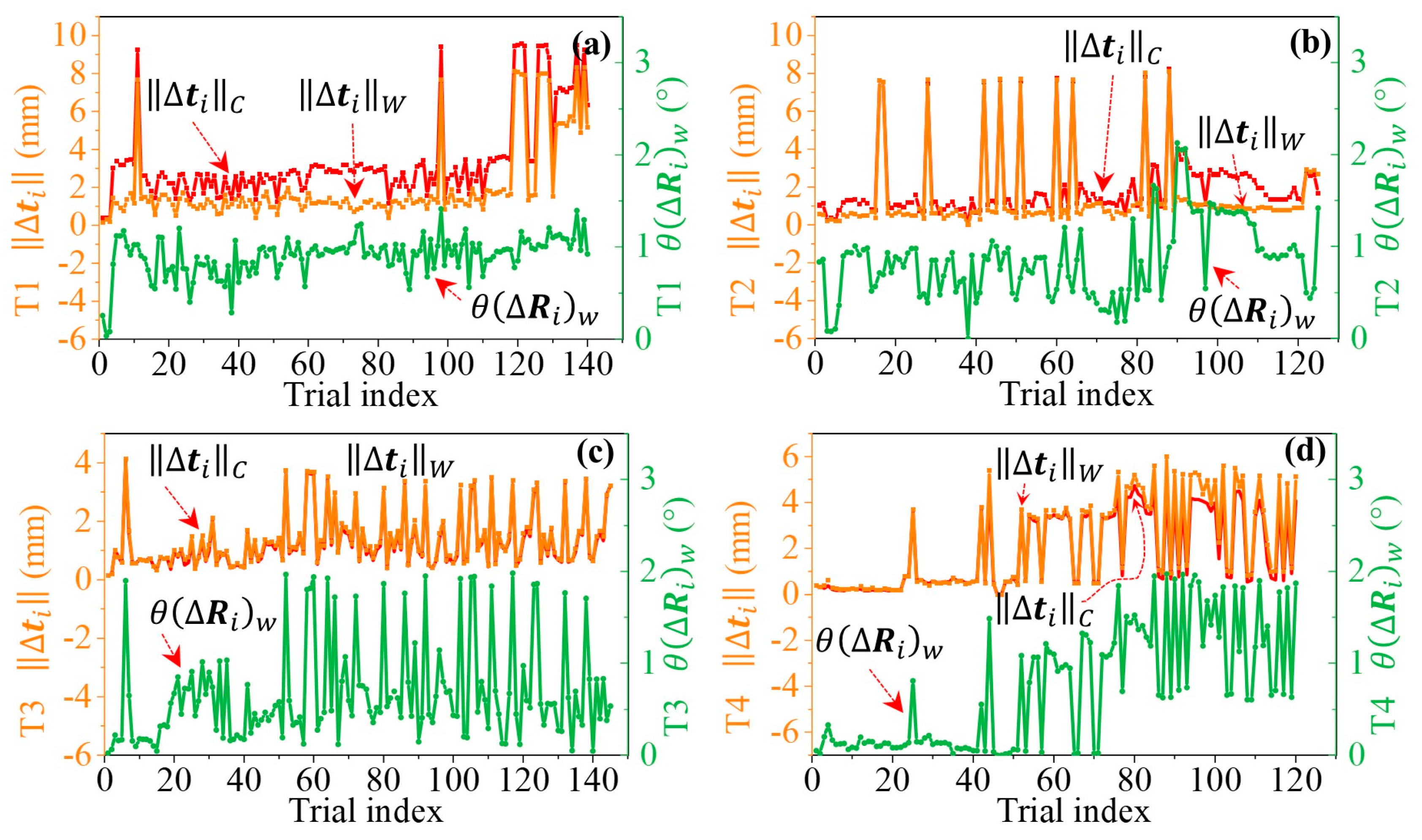
Trend of clamping error over repeated pickups. To investigate whether the clamping error exhibits a systematic increase over repeated use, potentially due to cumulative fixture wear or gripper jaw degradation, the quantities ‖∆t_i‖ and θ(∆R_i) were plotted against the pickup sequence index (i.e., the chronological trial order) for each blade type independently; the corresponding plots were shown in Figure 9 and Figure 10, respectively. Since each blade type was tested over a different time period, the pickup index provides a normalized measure of cumulative usage that enables consistent cross-type comparison.

Figure 9. Plots of ${‖∆{\mathit{t}}_i‖}_C$ and $\theta {\left(∆{\mathit{R}}_i\right)}_C$ against pickup index for each blade type. (a) T1; (b) T2; (c) T3; (d) T4.

Figure 10. Comparable plots of ${‖∆{\mathit{t}}_i‖}_C$, ${‖∆{\mathit{t}}_i‖}_W$, and $\theta {\left(∆{\mathit{R}}_i\right)}_W$ against pickup index for each blade type. (a) T1; (b) T2; (c) T3; (d) T4.

Fixture wear may exhibit step-like degradation after discrete damage events rather than gradual drift. The relationship between trial index and error magnitude is not expected to be linear. The Spearman rank correlation coefficient ρ was employed as a non-parametric measure of monotonic trend. Table 10 summarizes the half-split comparison and Spearman ρ for all four blade types. Since the trials were acquired sequentially with the same robot, fixture, and gripper, they are not independent samples; ρ is therefore reported as a descriptive measure of monotonic association rather than as an inferential test.

Table 10. Trend analysis of clamping error magnitude over repeated pickups.

Blade Type	N	${‖∆{\mathit{t}}_{\mathit{i}}‖}_{\mathit{C}}$ Mean (mm)			${‖∆{\mathit{t}}_{\mathit{i}}‖}_{\mathit{W}}$ Mean (mm)			Spearman ρ		p; 95% CI
		1st half	2nd half	All	1st half	2nd half	All	${‖∆{\mathit{t}}_i‖}_C$	${‖∆{\mathit{t}}_i‖}_W$	-
T1	140	2.47	4.30	3.38	1.26	2.81	2.03	+0.56	+0.48	9.6 × 10−13; [0.43, 0.66]
T2	125	1.76	2.27	2.02	1.35	1.37	1.36	+0.53	+0.58	1.5 × 10−10; [0.40, 0.65]
T3	145	1.16	1.43	1.30	1.23	1.51	1.37	+0.31	+0.31	1.5 × 10−4; [0.16, 0.45]
T4	120	0.92	2.86	1.89	0.96	3.35	2.16	+0.70	+0.74	3.8 × 10−19; [0.60, 0.78]

Notes: “1st half” and “2nd half” split the trial sequence at the median index. ρ is the Spearman rank correlation between trial index and error norm, with the p-value and 95% confidence interval from the Fisher z-transformation. Lag-1 autocorrelation/Durbin–Watson: 0.67/0.63, 0.01/1.99, 0.06/1.84, and 0.40/1.18 for T1–T4 (DW ≈ 2, no serial dependence).

As shown in Figure 9a–d and Table 10, the point-cloud displacement norm ${‖∆{\mathit{t}}_i‖}_C$ exhibited a statistically meaningful increasing trend for all blade types: T1 (ρ = +0.56), T2 (ρ = +0.53), T3 (ρ = +0.31), and T4 (ρ = +0.70). The corresponding workpiece error norm ${‖∆{\mathit{t}}_i‖}_W$ followed the same pattern with comparable Spearman coefficients, as shown in Figure 10a–d. The monthly breakdown further corroborates this trend: for T1, the mean ${‖∆{\mathit{t}}_i‖}_C$ rose from 0.31 mm (February 2025) to 2.64 mm (May 2025) and ultimately to 6.47 mm (January 2026); for T4, it progressed systematically from 0.25 mm (December 2024) to 2.94 mm (July 2025). T2 exhibited a milder increase, with the mean ${‖∆{\mathit{t}}_i‖}_C$ ranging from 0.81 mm to 2.30 mm over the observation period. These results are consistent with fixture and gripper jaw wear progressively degrading the repeatability of the clamping operation, and the magnitude of the error becomes substantial enough after several months of production to warrant online compensation. The wear itself was not measured, and no maintenance record was kept, so the association cannot be separated from elapsed time or from adjustments made to the cell during the campaign. All such inevitable errors are detectable and compensable by the online error compensation algorithm proposed in this work, which is a prerequisite for any long-term reliable automated grinding system.

(4)

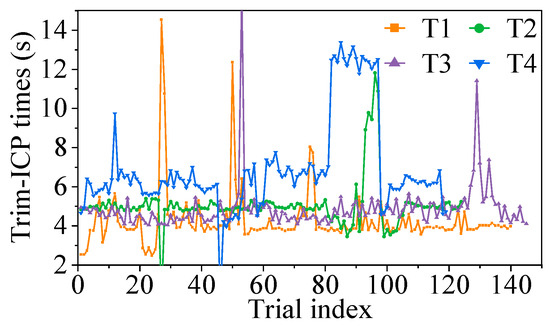
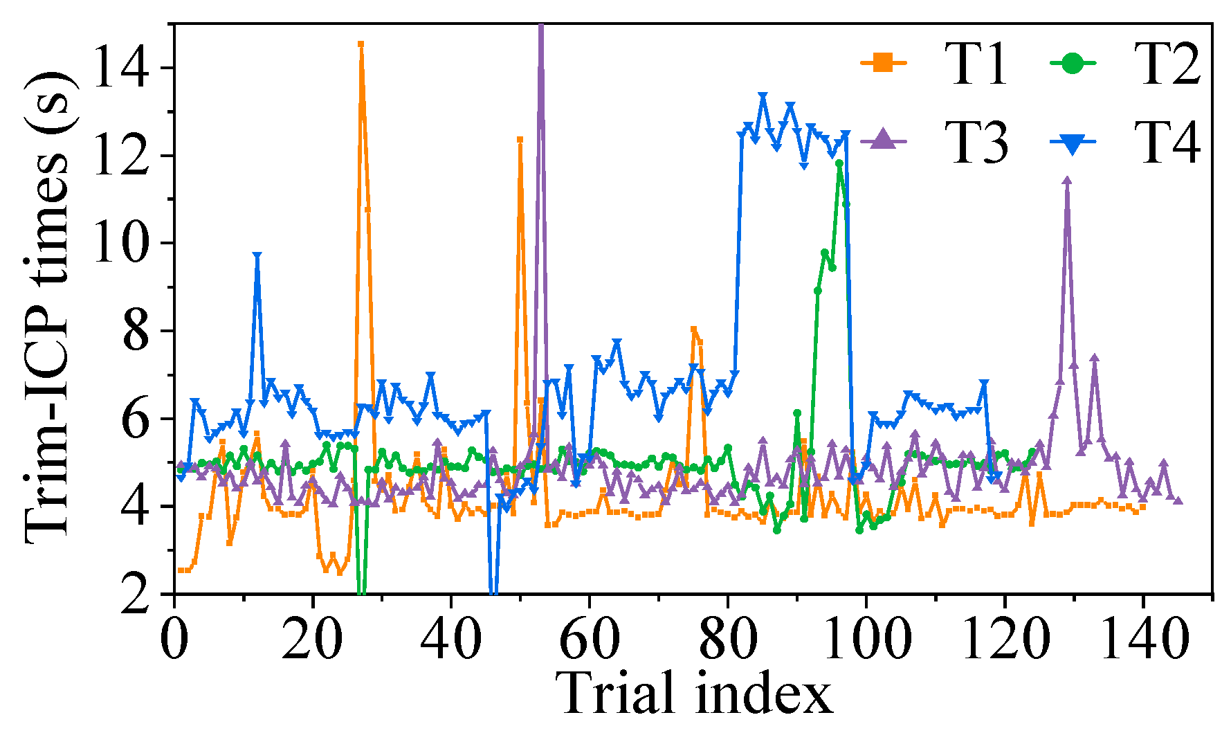
Analysis of registration time across trials. The total compensation pipeline time (point cloud loading, voxel downsampling, ICP registration, and pose update) was recorded for each trial. Figure 11 presents the ICP registration time for each clamping trial, plotted in chronological order for the four blade types (T1, T2, T3, T4). Across the 528 trials with a complete timing record, the registration time remained stable and showed no systematic increasing or decreasing trend with trial index, indicating consistent algorithmic performance throughout the entire production batch. The compensation adds no separate process step: it is executed at the scanning station during the dwell already required to acquire the scan, and the compensated pose is passed to the controller before the blade is moved to the grinding station.

Figure 11. Computation time trend over trial index for each blade type.

The computation time statistics are summarized in Table 11. The slightly higher mean time for T4 is attributed to its larger point-cloud size and more complex blade geometry, which increases the number of ICP iterations needed for convergence. The majority of trials exhibited registration times clustered tightly around their respective means, with standard deviations below 1.5 s for all blade types. Isolated data points with anomalously short registration times (e.g., 0.06 s for T4 and 0.08 s for T2) or moderately prolonged times (e.g., 14.5 s for T1 and 16.1 s for T3) were observed sporadically. These outliers are attributed to occasional system latency or abnormal interruption of the registration process rather than to any degradation of the ICP algorithm itself. Excluding these sporadic anomalies, the registration time remained within a narrow band of approximately 2.5~7.0 s for T1, 4.0~7.0 s for T2, 4.0~7.0 s for T3, and 4.5~10.0 s for T4, demonstrating that the proposed ICP-only compensation method is both computationally efficient and robust for online industrial deployment.

Table 11. ICP computation time statistics (seconds).

Blade Type	N	Mean (s)	Std (s)
T1	140	4.25	1.46
T2	124	5.04	1.23
T3	145	4.86	1.21
T4	119	6.92	2.41

Notes: two of the 530 valid trials were excluded from the timing statistics because their acquisition was interrupted, leaving the 528 trials reported here (124 for T2 and 119 for T4).

3.5. Coating Grinding Quality

To evaluate the practical effectiveness of the proposed clamping error compensation method, the coating thickness and surface roughness before and after robotic belt grinding were measured on production turbine blades. Because the YSZ thermal barrier coating must not be subjected to destructive testing, all measurements were performed non-destructively using a contact-type coating thickness gauge (Phynix Surfix, PHYNIX Sensortechnik GmbH, Neuss, Germany) and a portable surface roughness tester (Mitutoyo SJ-210, Mitutoyo Corporation, Kawasaki, Japan). Two complementary measurement campaigns were conducted: a spatially dense manual measurement on a small batch to validate removal uniformity, and a high-throughput automatic measurement on a large batch to establish statistical confidence in process consistency.

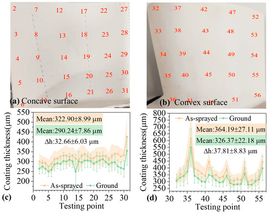
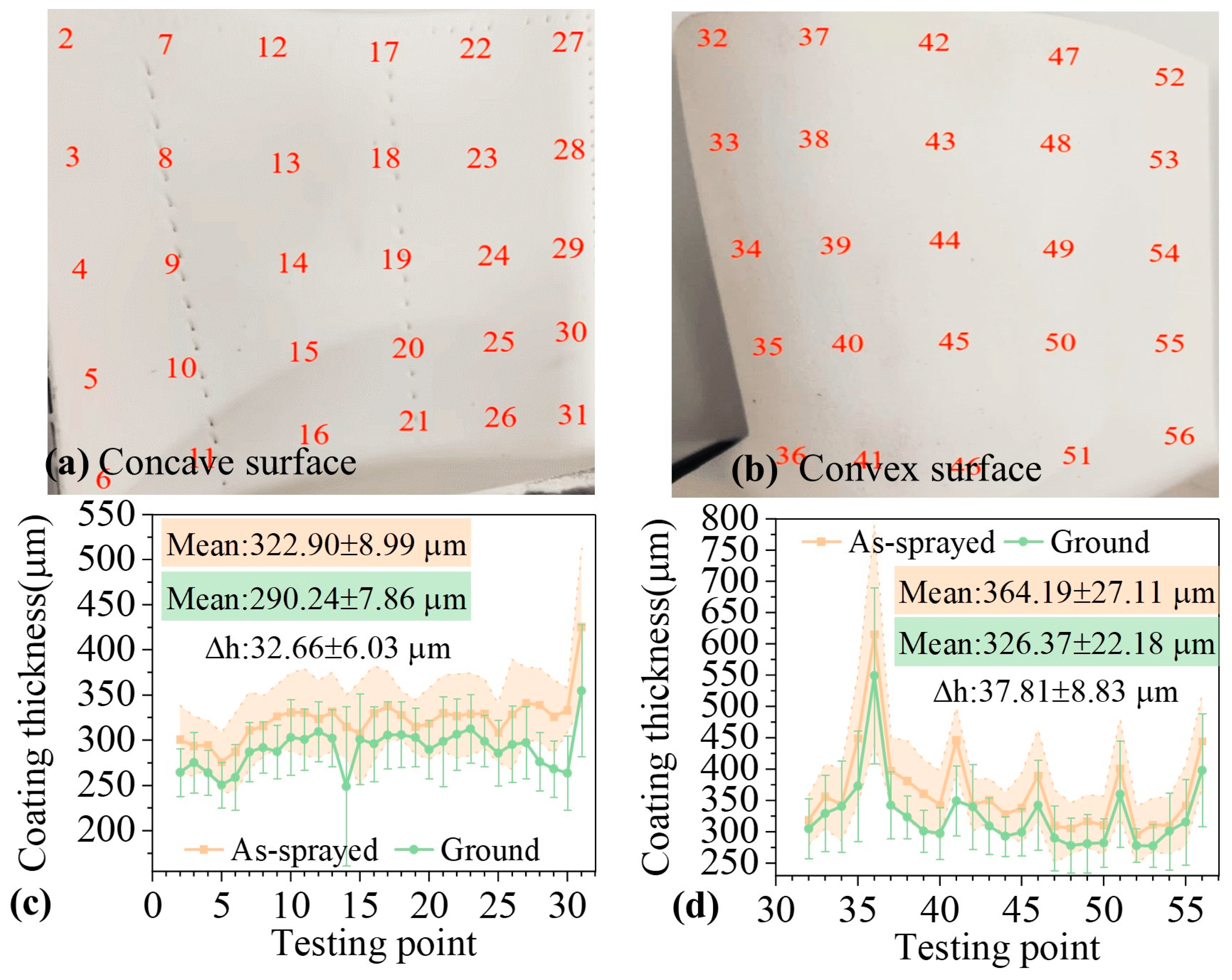
Manual measurement of coating thickness distribution. Six blades were manually measured at 56 predefined sampling points distributed across both the concave and convex surfaces, as illustrated in Figure 12a,b. The as-sprayed and post-grinding thickness values at each point, averaged over the six blades, are plotted in Figure 12c,d. On the concave side, the mean as-sprayed coating thickness was 322.90 ± 8.99 μm, which was reduced to 290.24 ± 7.86 μm after grinding, corresponding to a mean material removal of 32.66 ± 6.03 μm. On the convex side, the as-sprayed thickness was 364.19 ± 27.11 μm, reduced to 326.37 ± 22.18 μm, yielding a mean removal of 37.81 ± 8.83 μm. The final removal amounts on both sides differed by only approximately 5 μm, so that the removal was highly uniform across the geometrically asymmetric surfaces. Because all six blades were ground with the compensation active, this measurement establishes the uniformity achieved by the compensated process. Visual inspection of all ground surfaces under magnification confirmed a smooth, rounded morphology free of cracking, spallation, or over-grinding defects (Figure 12).

Figure 12. (a,b) Surface conditions and measurement locations on the concave and convex surfaces post-grinding. (c,d) Thickness distribution of the coating at the corresponding locations before and after grinding.

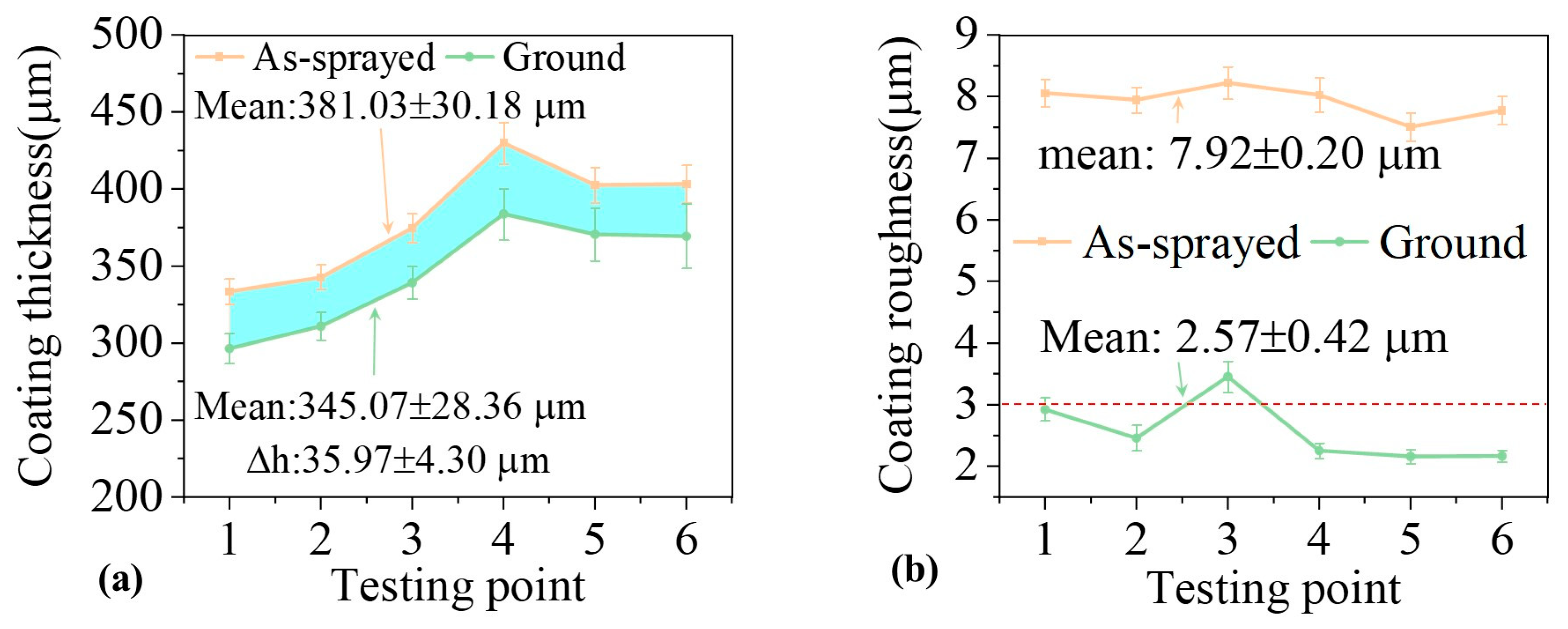
Statistical validation of thickness control and surface roughness. While the manual measurements provide spatially resolved thickness profiles, the per-point sample size (n = 6) limits the statistical power for assessing process repeatability. To address this, the automated measurement capability integrated into the grinding system was employed to record the coating thickness and surface roughness at six fixed locations (three on each of the concave and convex surfaces) on 118 consecutively processed T1 blades. The automated positioning ensures that the identical physical location is measured on every blade, thereby capturing the true blade-to-blade variation. The summarized results are presented in Figure 13.

Figure 13. (a) Thickness and (b) surface roughness of YSZ coatings before and after grinding (data from 118 T1 blades).

The mean coating thickness removal across all 118 T1 blades was 35.97 ± 4.30 μm, which agrees closely with the manual measurement results (32.66~37.81 μm) and confirms the stability of the material removal process under the proposed compensation scheme. With respect to surface quality, the grinding process produced a substantial improvement: the mean surface roughness Ra decreased from 7.92 ± 0.20 μm in the as-sprayed condition to 2.57 ± 0.42 μm after grinding, corresponding to an average reduction of 5.35 ± 0.27 μm. The industrial acceptance criterion requires the roughness at each measurement location to be below Ra 3.0 μm. Five of the six locations met it; the sixth, on the convex surface, averaged 3.45 μm over the 118 blades and exceeded it, while the overall distribution remained tightly concentrated around the mean. Furthermore, no instances of coating delamination, excessive thinning below the minimum allowable thickness, or incomplete coverage were observed across the entire batch. What the compensation acts upon is the placement of the tool path rather than the roughness produced by the abrasive itself. An uncompensated path deviation of millimeters is therefore two orders of magnitude larger than the removal depth, which would place the tool outside the intended cut for a large part of the airfoil. This establishes that compensation is a necessary condition for the observed removal uniformity, although the absolute roughness level is governed by the abrasive specification and process parameters.

The manual and automatic measurements show that the system, operating with the proposed compensation, achieved (i) uniform coating removal across both concave and convex surfaces, (ii) surface roughness within the design specification at five of the six measurement locations, and (iii) these metrics were maintained over a production run of more than one hundred T1 blades. Because no uncompensated control group was available, the results characterize the compensated process as a whole rather than isolating the contribution of the compensation.

A limitation of this research is the absence of a control group. The ideal design would comprise at least three groups, grinding without online compensation, grinding after conventional coarse-to-fine manual registration, and the proposed reference-scan method, so that the effect on coating quality could be isolated. This was not possible on the commissioned cell, and the comparison is therefore listed as the primary item of future work.

4. Discussion

4.1. Forward Error Propagation Modeling

The trajectory error is separated into three levels: the localization error, i.e., the error in the estimated workpiece pose; the trajectory command error, i.e., the error remaining at the tool once the localization error has been transferred to the path; and the surface tool error, contributed by the process itself through the deviation of the blade from its nominal shape and the geometric and wear state of the abrasive tool. This model addresses the first level, for which four sources are identified, as summarized in Table 12. They originate in physically distinct subsystems and are identified by separate measurement channels, so they are treated as uncorrelated; only ${\epsilon }_{\mathit{clamp}}^i$ varies per blade pickup, the other three being approximately constant within a batch. Each is bounded and small enough for a first-order treatment.

Table 12. Error sources in the robotic grinding system.

Symbol	Error Pose	Source	Nature	Typical Magnitude	Compensated?
εh	δTh	Hand-eye calibration error	Systematic, slowly drifting	≈0.1 mm ≈0.05 deg	No
εc	δTc	Initial blade poses calibration error	Systematic	≈(0.1~0.3) mm	No
εk	δTk	Robot kinematic error	Systematic	≈(0.3~1.0) mm	No
${\epsilon }_{\mathit{clamp}}^i$	ΔTclamp	i-th clamping error	Random (per pickup)	Bounded by fixture and gripper tolerances; increases with wear	Yes

The total post-compensation trajectory error is dominated by three systematic sources:

$${\epsilon }_{\mathit{total}}^2\cong {\epsilon }_h^2+{\epsilon }_c^2+{\epsilon }_k^2$$

(15)

Equation (15) is a conservative bound rather than a variance sum, because the three terms are bounded systematic offsets rather than zero-mean random variables. The clamping error is thereby decoupled from the error budget, converting a random per-blade error into a systematic per-batch error determined by calibration quality; the rotation–translation interaction is treated at the waypoint level in Equation (20).

For a trajectory waypoint ${}^{W_0}P_w$ in {W₀}, the nominal position in {E} is:

$${}^{E}P_{w,\mathit{no}}={}_B{}^E\mathit{T}\cdot {}_L{}^B\mathit{T}\cdot {}_{C_0}{}^{\mathrm{L}}\mathit{T}\cdot {}_{W_0}{}^{C_0}\mathit{T}\cdot {}^{W_0}P_w={}_B{}^E\mathit{T}\cdot {}_L{}^B\mathit{T}\cdot {}_{W_0}{}^{C_0}\mathit{T}\cdot {}^{W_0}P_w$$

(16)

The actual position without compensation is:

$${}^{E}P_{w,\mathit{uncomp}}=\left(\delta {\mathit{T}}_k\cdot {}_B{}^E\mathit{T}\right)\cdot \left(\delta {\mathit{T}}_h\cdot {}_L{}^B\mathit{T}\right)\cdot \left(\Delta {\mathit{T}}_{\mathit{clamp}}\right)\cdot \left(\delta {\mathit{T}}_c\cdot {}_{W_0}{}^{C_0}\mathit{T}\right)\cdot {}^{W_0}P_w$$

(17)

With compensation, using the ICP estimate ${}_{C_i}{}^{C_0}\mathit{T}$:

$${}^{E}P_{w,\mathit{comp}}=\left(\delta {\mathit{T}}_k\cdot {}_B{}^E\mathit{T}\right)\cdot \left(\delta {\mathit{T}}_h\cdot {}_L{}^B\mathit{T}\right)\cdot (\Delta {\mathit{T}}_{\mathit{clamp}}\cdot {}_{C_i}{}^{C_0}\mathit{T})\cdot \left(\delta {\mathit{T}}_c\cdot {}_{W_0}{}^{C_0}\mathit{T}\right)\cdot \left({}^{W_0}P_w\right)$$

(18)

4.2. Compensation Error Analysis

The uncompensated trajectory error is dominated by the clamping displacement. Although the true clamping error ΔT_clamp, in Equation (17), cannot be directly measured in the industrial setting without auxiliary metrology equipment, its magnitude is estimated by ICP as $‖\widehat{\Delta t}‖$, the translational norm of the ICP output. The uncompensated position error at any trajectory waypoint is therefore:

$$e_{\mathit{uncomp}}\cong ‖\widehat{\Delta t}‖$$

(19)

After applying the compensation transformation ${}_{C_i}{}^{C_0}\mathit{T}$ according to Equation (18), the residual error arises from the imperfect cancellation $\Delta {\mathit{T}}_{\mathit{clamp}}\cdot {}_{C_i}{}^{C_0}\mathit{T}\ne \mathit{I}$. Since both P_i and P_ref are acquired by the same sensor under identical viewing conditions, the residual misalignment is characterized by the ICP convergence residual.

Let ε_fit denote the RMS fitness score at ICP convergence, the root-mean-square point-to-point distance between P_i and P_ref after registration, directly reported by the ICP solver. Let θ_res denote the residual angular error of the imperfect cancellation. For a trajectory waypoint ${}^{W_0}P_w$ at distance $r=‖{}^{W_0}P_w‖$ from the workpiece frame origin, the compensated position error is bounded by:

$$e_{\mathit{comp}}\left({}^{W_0}P_w\right)\le {\epsilon }_{\mathit{fit}}+r\sin \left({\theta }_{\mathit{res}}\right)$$

(20)

The first term, ε_fit, accounts for the translational residual that affects all waypoints uniformly. The second term, rsin(θ_res), captures the amplification of residual rotation with distance from the origin: a small angular error produces a proportionally larger positional deviation at the blade tip than near the root. The residual angular error θ_res can be estimated from the repeatability of the ICP rotation estimates. Over N repeated clamping trials, the per-axis standard deviations of the Euler angles extracted from $\widehat{\Delta R_i}$ characterize the angular estimation precision. Taking the root-sum-of-squares of these standard deviations as θ_res yields a conservative upper bound. The compensation effectiveness is quantified by the error reduction ratio. Here, the ratio is evaluated from the mean error magnitudes rather than as the average of the per-trial ratios, which is ill-conditioned when the denominator is small.

$$\eta ={\displaystyle \frac{e_{\mathit{uncomp}}-e_{\mathit{comp}}}{e_{\mathit{uncomp}}}}\times 100\%$$

(21)

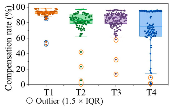
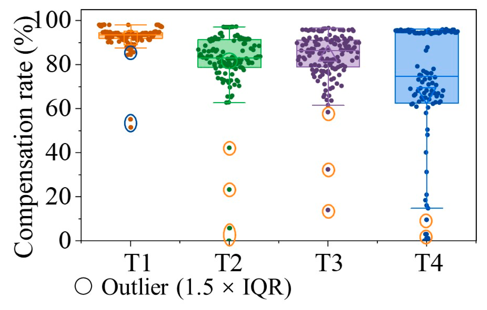
Figure 14 presents the compensation rate as a function of trial index for the four blade types, comprising 530 valid clamping trials in total. The mean compensation rate exceeded 89% for all four blade types, with values of 94.7% (T1, 140 trials), 89.0% (T2, 125 trials), 89.6% (T3, 145 trials) and 90.1% (T4, 120 trials). For the vast majority of trials, the compensation rate exceeded 70%, indicating that the online compensation consistently removed the dominant component of the clamping error. The lower mean rate for T4 is attributed to its relatively small uncompensated error (mean 1.89 mm combined with a blade radius r = 160 mm), which leaves less absolute margin for improvement once the fixed residual bound e_comp is accounted for. Isolated trials exhibiting negative or near-zero compensation rates correspond to cases where the measured clamping error (e.g., below 0.2 mm) was already comparable to the compensation residual bound, i.e., the clamping repeatability was so high that the uncompensated error was already at the level of the measurement uncertainty. These cases are not indicative of compensation failure but rather reflect the physical limit of achievable accuracy. Table 13 summarizes the aggregate statistics of the uncompensated clamping error, the compensated residual and the compensation ratio for the four blade types, including the root-mean-square and mean absolute errors, the 95th percentile and the fraction of trials within a given tolerance. The uncompensated clamping error varies by more than an order of magnitude between pickups, as the tolerance fractions in Table 13 show. The compensated residual e_comp lies between 0.135 mm and 0.223 mm for all four blade types.

Figure 14. Boxplot of the compensation rate η for the four blade types. Notes: the box spans the interquartile range, the horizontal line is the median, and the whiskers extend to the most extreme values within 1.5 × IQR.

Table 13. Clamping error and compensation statistics over 530 valid pickup trials.

Blade Type	N	euncomp Mean ± SD (mm)	RMSE (mm)	MAE (mm)	P95 (mm)	Max (mm)	euncomp (mm)	η (%)
T1	140	3.383 ± 2.215	4.039	3.383	9.438	9.607	0.179	94.7
T2	125	2.020 ± 1.845	2.731	2.020	7.568	8.226	0.223	89.0
T3	145	1.297 ± 0.937	1.598	1.297	3.363	4.061	0.135	89.6
T4	120	1.888 ± 1.695	2.532	1.888	4.461	4.844	0.188	90.1
All	530	2.152 ± 1.896	2.867	2.152	7.000	9.607	-	91

Notably, the compensation rate showed no correlation with trial index, so compensation performance did not degrade as the fixture wore. This is not in conflict with the increase in the raw clamping error: e_uncomp reflects the mechanical interface and grows with wear, whereas e_comp is bounded by the registration precision, independently of the magnitude corrected. The method thus converts a random per-pickup error of up to several millimeters into a calibration-bound residual an order of magnitude smaller.

5. Conclusions

This paper presented an automated clamping error compensation method for robotic grinding of turbine blade thermal barrier coatings, addressing the bottleneck of manual coarse registration in batch production. The core innovation is a reference-scan-based registration strategy: the first blade in each batch is calibrated once with manual assistance, and the resulting reference point cloud is subsequently used to localize every new pickup through Trimmed-ICP fine registration alone. Because clamping errors are bounded by the mechanical constraints of the gripper and fixture system and therefore lie inside the ICP convergence basin, coarse registration is no longer required, converting a manual, operator-dependent step into a fully automated procedure.

The main contributions are threefold. First, the reference-based ICP framework eliminates the coarse registration bottleneck and enables full automation of the batch production workflow. Second, an error propagation model quantitatively demonstrates that the proposed compensation decouples the random per-pickup clamping error from the systematic calibration error budget, so that the localization component of the trajectory error is governed by calibration quality rather than by the clamping operation. Third, extensive experiments validate the method across 530 pickup trials on four blade types, achieving a mean compensation rate of 91%, post-compensation residuals below 0.2 mm, and a valid-registration rate of 98.5% (530 of 538 records) with no solver failures. Coating quality assessment on 118 T1 blades further confirms uniform thickness removal, with Ra ≤ 3.0 μm met at five of six measurement locations (one convex-side location reached 3.45 μm).

The method has three limitations: it requires one manual coarse registration per batch, the blade geometry must remain unchanged between the reference and compensation scans, and the reference scan must provide sufficient geometric coverage to constrain all six degrees of freedom. Independent validation is limited, because no CMM, laser tracker, or photogrammetric system was available in the commissioned cell and no uncompensated control group could be produced after hand-over. Future work will investigate deep-learning-based methods for fully automatic initial coarse registration, extend the framework to in-process re-scanning during grinding, and integrate and develop information-theoretic metrics for optimal reference scan path selection.

References

- Pisarenko, Z.; Simchenko, N.; Ivanov, L.; Xie, W.; Nasyrova, G. Prerequisites, opportunities and risks for the future development of nanotechnology at the global level. Nanotechnol. Constr. A Sci. Internet-J. 2025, 17, 775–786. [Google Scholar] [CrossRef] [Scilit]
- Li, Z.; Qu, S.; Sun, Y.; Gong, Y.; Chu, D.; Yao, P.; Li, Z.; Xu, X. Robot grinding: From frontier hotspots to key technologies and applications. Intell. Sustain. Manuf. 2025, 2, 10027. [Google Scholar] [CrossRef] [Scilit]
- Zhu, D.; Feng, X.; Xu, X.; Yang, Z.; Li, W.; Yan, S.; Ding, H. Robotic grinding of complex components: A step towards efficient and intelligent machining-challenges, solutions, and applications. Robot. Comput.-Integr. Manuf. 2020, 65, 101908. [Google Scholar] [CrossRef] [Scilit]
- Basak, A.; Celis, J.-P.; Vardavoulias, M.; Matteazzi, P. Effect of nanostructuring and Al alloying on friction and wear behaviour of thermal sprayed WC-Co coatings. Surf. Coat. Technol. 2012, 206, 3508–3516. [Google Scholar] [CrossRef] [Scilit]
- Chen, T.; Dong, S.; Cai, Z.; Deng, C.; Cao, X. Study on robot trajectory planning and coating thickness prediction for plasma spraying on complex surface. J. Manuf. Process. 2024, 131, 1046–1060. [Google Scholar] [CrossRef] [Scilit]
- Yang, F.; Cai, Z.; Chen, Y.; Dong, S.; Deng, C.; Niu, S.; Zeng, W.; Wen, S. A robotic polishing trajectory planning method combining reverse engineering and finite element mesh technology for aero-engine turbine blade TBCs. J. Therm. Spray Technol. 2022, 31, 2050–2067. [Google Scholar] [CrossRef] [Scilit]
- Chen, Z.; Cai, Z.; Chen, T.; Deng, C.; Niu, S.; Wang, C.; Qu, D.; Ma, Z.; Hu, Y. A non-contact calibration method of workpiece coordinate system for aero-engine blade-robotic grinding system. Proc. Inst. Mech. Eng. Part B J. Eng. Manuf. 2025, 239, 1994–2006. [Google Scholar] [CrossRef] [Scilit]
- Liang, X.; Cai, Z.; Zeng, C.; Mu, Z.; Li, Z.; Yang, F.; Chen, T.; Dong, S.; Deng, C.; Niu, S. A robotic polishing trajectory planning method for TBCs of aero-engine turbine blade using measured point cloud. Ind. Robot Int. J. Robot Res. Appl. 2022, 50, 275–286. [Google Scholar] [CrossRef] [Scilit]
- Li, J.; Chen, M.; Jin, X.; Chen, Y.; Dai, Z.; Ou, Z.; Tang, Q. Calibration of a multiple axes 3-D laser scanning system consisting of robot, portable laser scanner and turntable. Optik 2011, 122, 324–329. [Google Scholar] [CrossRef] [Scilit]
- Tabb, A.; Ahmad Yousef, K.M. Solving the robot-world hand-eye(s) calibration problem with iterative methods. Mach. Vis. Appl. 2017, 28, 569–590. [Google Scholar] [CrossRef] [Scilit]
- Zhang, Z. A flexible new technique for camera calibration. IEEE Trans. Pattern Anal. Mach. Intell. 2000, 22, 1330–1334. [Google Scholar] [CrossRef] [Scilit]
- Usamentiaga, R.; García, D.F.; Molleda, J. Efficient registration of 2D points to CAD models for real-time applications. J. Real-Time Image Process. 2018, 15, 329–347. [Google Scholar] [CrossRef] [Scilit]
- Rusu, R.B.; Blodow, N.; Marton, Z.C.; Beetz, M. Aligning point cloud views using persistent feature histograms. In Proceedings of the 2008 IEEE/RSJ International Conference on Intelligent Robots and Systems, Nice, France, 22–26 September 2008; pp. 3384–3391. [Google Scholar] [CrossRef] [Scilit]
- Rusu, R.B.; Blodow, N.; Beetz, M. Fast Point Feature Histograms (FPFH) for 3D registration. In Proceedings of the 2009 IEEE International Conference on Robotics and Automation, Kobe, Japan, 12–17 May 2009; pp. 3212–3217. [Google Scholar] [CrossRef] [Scilit]
- Aiger, D.; Mitra, N.J.; Cohen-Or, D. 4-points congruent sets for robust pairwise surface registration. In Proceedings of the SIGGRAPH ‘08: Special Interest Group on Computer Graphics and Interactive Techniques Conference, Los Angeles, CA, USA, 11–15 August 2008; Volume 27, pp. 1–10. [Google Scholar] [CrossRef] [Scilit]
- Mellado, N.; Aiger, D.; Mitra, N.J. Super 4PCS: Fast global pointcloud registration via smart indexing. Comput. Graph. Forum 2014, 33, 205–215. [Google Scholar] [CrossRef] [Scilit]
- Yang, J.; Li, H.; Campbell, D.; Jia, Y. Go-ICP: A globally optimal solution to 3D ICP point-set registration. IEEE Trans. Pattern Anal. Mach. Intell. 2016, 38, 2241–2254. [Google Scholar] [CrossRef] [Scilit]
- Yang, H.; Shi, J.; Carlone, L. TEASER: Fast and certifiable point cloud registration. IEEE Trans. Robot. 2021, 37, 314–333. [Google Scholar] [CrossRef] [Scilit]
- Besl, P.J.; McKay, N.D. Method for registration of 3-D shapes. IEEE Trans. Pattern Anal. Mach. Intell. 1992, 14, 239–256. [Google Scholar] [CrossRef] [Scilit]
- Rusinkiewicz, S.; Levoy, M. Efficient variants of the ICP algorithm. In Proceedings of the International Conference on 3-D Digital Imaging and Modeling, Quebec City, QC, Canada, 28 May–1 June 2001; pp. 145–152. [Google Scholar] [CrossRef] [Scilit]
- Segal, A.; Haehnel, D.; Thrun, S. Generalized-ICP. Robotics: Science and Systems 2009. Available online: https://api.semanticscholar.org/CorpusID:231748613 (accessed on 1 September 2026).
- Serafin, J.; Grisetti, G. NICP: Dense normal based point cloud registration. In Proceedings of the 2015 IEEE/RSJ International Conference on Intelligent Robots and Systems (IROS), Hamburg, Germany, 28 September–2 October 2015; pp. 742–749. [Google Scholar] [CrossRef] [Scilit]
- Pomerleau, F.; Colas, F.; Siegwart, R.; Magnenat, S. Comparing ICP variants on real-world data sets. Auton. Robots 2013, 34, 133–148. [Google Scholar] [CrossRef] [Scilit]
- Nubiola, A.; Bonev, I.A. Absolute calibration of an ABB IRB 1600 robot using a laser tracker. Robot. Comput.-Integr. Manuf. 2013, 29, 236–245. [Google Scholar] [CrossRef] [Scilit]
- Lightcap, C.; Hamner, S.; Schmitz, T.; Banks, S. Improved positioning accuracy of the PA10-6CE robot with geometric and flexibility calibration. IEEE Trans. Robot. 2008, 24, 452–456. [Google Scholar] [CrossRef] [Scilit]
- Zhou, P.; Zhou, Y.; Xie, Q.; Zhao, H. Adaptive force control for robotic grinding of complex blades. IOP Conf. Ser. Mater. Sci. Eng. 2019, 692, 012008. [Google Scholar] [CrossRef] [Scilit]
- Li, Z.; Sun, H.; Yang, J.; Ding, H. High-accuracy compensation for profile errors in robotic compliant grinding by force adjustment. J. Manuf. Process. 2025, 157, 411–423. [Google Scholar] [CrossRef] [Scilit]
- Moeller, C.; Schmidt, H.C.; Koch, P.; Boehlmann, C.; Kothe, S.; Wollnack, J.; Hintze, W. Real time pose control of an industrial robotic system for machining of large scale components in aerospace industry using laser tracker system. SAE Int. J. Aerosp. 2017, 10, 100–108. [Google Scholar] [CrossRef] [Scilit]
- Ge, J.; Deng, Z.; Wang, S.; Li, Z.; Liu, W.; Nie, J. Vision Sensing-Based Online Correction System for Robotic Weld Grinding. Chin. J. Mech. Eng. 2023, 36, 125. [Google Scholar] [CrossRef] [Scilit]
- Chetverikov, D.; Svirko, D.; Stepanov, D.; Krsek, P. The trimmed iterative closest point algorithm. In Proceedings of the International Conference on Pattern Recognition, Quebec City, QC, Canada, 11–15 August 2002; Volume 3, pp. 545–548. [Google Scholar] [CrossRef] [Scilit]
Disclaimer/Publisher’s Note: The statements, opinions and data contained in all publications are solely those of the individual author(s) and contributor(s) and not of MDPI and/or the editor(s). MDPI and/or the editor(s) disclaim responsibility for any injury to people or property resulting from any ideas, methods, instructions or products referred to in the content. |
© 2026 by the authors. Licensee MDPI, Basel, Switzerland. This article is an open access article distributed under the terms and conditions of the Creative Commons Attribution (CC BY) license.