


Abstract
Hwang developed inventory models with amelioration items and applied the graphical method to locate the optimal solution. In this study, we derive an analytical method to find two local maximum points and one local minimum point. Our maximum profit is greatly superior to that of Hwang, because his maximum profit is about 0.246% of ours. The local maximum point near the starting point (denoted as ) is almost impossible to discoverby the numerical method, illustrating the effectiveness of our analytical method.
MSC:
90B05
1. Introduction
Hwang [1] was the first to study the amelioration effect for inventory models. He constructed two inventory systems, (i) the Economic Ordering Quantity (EOQ) model and (ii) the Partially Selling Quantity (PSQ) model, with ameliorated items such that the storage items will self-reproduce, for example, like fish being raised in a closed pond. After his publication, Hwang [1] has been cited 163 times, indicating that many researchers paid attention to this topic of interest. However, most of them concentrated on their new models, and they, therefore, did not examine Hwang [1] in detail. For example, Malekitabar et al. [2] developed a two-echelon inventory system, consisting of a supplier and a farmer with a feeding function for rainbow trout, and Hwang [1] only appeared once in their Introduction.
There are only two papers that studied Hwang [1] with respect to his solution procedure: Chou et al. [3] and Tuan et al. [4]. Chou et al. [3] examined the EOQ model proposed by Hwang [1] under the restriction , where the purchase cost is greater than the amelioration cost, to derive an inclusiveresolution procedure. Tuan et al. [4] also studied the EOQ model proposed by Hwang [1], under the restriction , where the purchase cost is less than the amelioration cost. Depending on (a) , (b) , and (c) , Tuan et al. [4] obtained a complete solution structure.
Consequently, up untilnow, no papers have further discussed the PSQ model proposed by Hwang [1]. To fulfill this research gap, in this study, we will provide a rigorous mathematical procedure to find all local extreme points: two local maximum points and one local minimum point to enhance the graphical method proposed by Gupta [5], and then applied by Hwang [1].
The main contribution of this paper is twofold. First, we will provide a solid mathematical algorithm to find all critical points for the objective function studied by Hwang [1], and then decide on a local minimum point and two local maximum points. Second, we will illustrate that purely applying a numerical algorithm to search for the global maximum point is not reliable to demonstrate the effectiveness of the analytical algorithm.
This study is organized as follows. We briefly review those related papers of Hwang [1], Chou et al. [3], and Tuan et al. [4] in Section 1. We introduce notation and assumptions in Section 2. We provide a brief reviewing for solution algorithms of related papers in Section 3. We develop our new solution algorithm in Section 4 to derive two local maximum points and one local minimum point. We study the same numerical example proposed by Hwang [1] in Section 5 to indicate that our resultshows a significantimprovementoverthat of Hwang [1]. In Section 6, we point out that relying solely on a numerical algorithm to locate the global maximum point without prior analytical investigation may result in certain local extreme points being overlooked. We conclude our discussion in Section 8.
2. Notation and Assumptions
We use the same notation as Hwang [1] with several of our proposed new expressions. To shorten the formula expression, we define five new auxiliary functions: , , , , and .
is related to the first derivation of the objective function. is related to the first derivation of . The purpose of , and is to present a solvable solution algorithm.
, , and are related to the sign of , helping us to solve .
These notations of the partial selling quantity model of Hwang [1] and our new assumptions are listed in the following.
denotes the amelioration rate with (1/day) where denotes the scale parameter and denotes the shape parameter.
denotes the average total profit per unit time that consists of selling revenue, ordering cost, holding cost, and the ameliorating cost for our second (₩/day).
denotes the total amelioration amount, with
where is the amelioration amount during the time interval .
denotes an auxiliary function, with
denotes another auxiliary function to simplify the derivations and help us to locate the solution of , with
denotes another auxiliary function to simplify the derivations and help us to locate the solution of , with
denotes the amelioration cost (₩/kg).
denotes the holding cost (₩/kg/day).
denotes the ordering cost (₩).
denotes an auxiliary function, with
such that .
denotes a second auxiliary function, with
such that .
denotes the inventory level (kg).
denotes the selling price per item.
denotes the constant demand rate (kg/day).
denotes the extra quantity to be sold at , with .
denotes the parameter to denote the time of amelioration (day).
denotes the cycle time (day).
denotes the solution of , for .
denotes the solution of , for and , which are critical points for the objective function, with and , and with . We will show that and are local maximum points, and is a local minimum point.
denotes the optimal solution (day). We will derive the following: .
3. Review of the Related Model
ThePSQ model starts with an initial inventory level, , and the amelioration effect causes the inventory level to continuously increase. Since the holding cost increases with the inventory level, the extra accumulated production is sold at in an amount of . At time , the next replacement cycle begins with an initial inventory level of .
The inventory model with amelioration items satisfies the differential equation with respect to the inventory level:
denotes the scale parameter and denotes the shape parameter that followsthe Weibull distribution for amelioration items, where denotes the demand rate.
With the integration factor , we obtain the next result:
such that we multiplyboth sides of Equation (1) by to both sides of Equation (1) toderive
We compare Equations (2) and (3), and then takethe integration to show that
where is the integration constant.
According to Equation (4), we derive that . Hwang [1] studied the partial selling quantity model under the restriction .
We obtain
and
under the restriction
We compute the followingholding cost:
with the purchasing cost, , and the setup cost, .
Inthe previous three related papers of Hwang [1], Chou et al. [3], and Tuan et al. [4], all of them applied an approximated holding cost as follows,
In the following, we explain the amelioration phenomenon. For a small time interval, denoted as , we designate the amelioration amount as and then we show that
The total amelioration amountis denoted as , and then
According to Equation (10), we rewrite Equation (11) as follows:
We recall the mean value theorem (Thomas and Finney [6]) to rewrite Equation (12) as follows:
where is a point in the small interval .
We can convert the Riemann sum of Equation (13) into a finite integration such that
According to Equation (14), the amelioration cost is evaluated as
Hwang [1] developed his partial selling quantity modelto maximize the average total profit. We refer to his objective function:
We must point out that the goal is to maximize the average total profit, such that the notation of “TC” in Equation (16) is questionable. Hence, we change from “TC” to “ATP”.
We recall Equation (6) to derive the following objective function:
with
We will present our solution algorithm in the next section.
4. Our New Solution Algorithm
We plug Equation (18) into Equation (17) to obtain the following objective function:
The partial selling quantity model proposed by Hwang [1] satisfies the restriction with the extra quantity to be sold at .
We recall the numerical example proposed by Hwang [1], with , , , , , , , and , and we evaluate to derive
We consult the work ofHwang [1], finding that, owing to the graphical method proposed by Gupta [5], he derived ( is revised to ) and .
According to Equation (19), we derive
revealingthat the estimation proposed by the graphical method of Gupta [5] is not accurate, whichmotivates us to study Hwang [1] in detail.
We observe Equation (17) to solve , implying that
If , then that results in
and then, we imply that
We compare Equations (20), (21) and (24) to conclude that if ,
Hence, we can reduce our domain from , an infinite domain, to a finite domain:
We summarize our results in the following lemma.
Lemma 1.
The searching domain is reduced from an infinite region to a finite region . The maximum problem becomes solvable.
Based on Equation (19), we derive
where is an auxiliary function to simplify the expression, with
We thendetermine the intervals that are positive or negative for . If we directly study , further examination becomes too difficult.
Thus, we consider an auxiliary function, , that has the same sign as .
According to Equation (28), we obtain
where is a second auxiliary function to simplify the expression, with
We thendecide the positive or negative intervals for . If we directly study , further examination becomes too difficult.
Thus, we consider another auxiliary function, , that has the same sign as .
Motivated by Equation (30), we assume the third auxiliary function, denoted as , such that
We derive , and , and then we can claim that if , then .
To simplify the expression, we define
We try to solve , and then we evaluate
such that if , then
We begin to show that , for .
On the other hand, we compute at to derive
We define another auxiliary function, denoted as , with
and then we define as the solution of to obtain
and then we derive .
For , we know that
Thus, we combine Equations (32), (34), (36) and (37) to derive
for .
We compute
and
Consequently, for , referring to Equations (32), (35), (36), (40) and (41), we evaluate
Therefore, we derive
for .
We combine our results of Equations (39) and (43) to derive the next lemma.
Lemma 2.
When Hence, we can shrink the searching region for .
According to Lemma 2, we reduce the examining domain of from to .
We compute that , and , and then we test whether or not there is a positive value for ; nextwe find that .
Hence, we derive that has two solutions, denoted as and , with , and . We estimate that
and
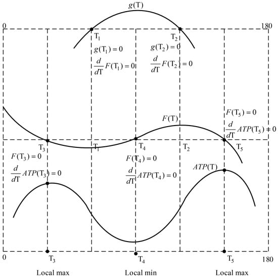
Please refer to Figure 1 at the end of this paper, at the upper picture, for the graph of to show which shows that , and are the two zeros of . will be a local minimum point for , and will be a local maximum point for . From the sign of , we know the monotonic properties of .
Figure 1.
The upper picture: . The middle picture: . The lower picture: .
We summarize our findings in the next lemma.
Lemma 3.
We prove that has two solutions, denoted as , and , with .
Thus, we obtain that for , and , . On the other hand, for , .
We recall Equation (29); it shows that and have the same sign, implying that for , and , .
On the other hand, for , .
Hence, we derive that is a decreasing function for , and . On the other hand, for , is an increasing function.
Consequently, we evaluate that , , , and .
Therefore, we know that F have hasthree solutions, denoted as ,, and , such that , , and ; we derive the following:
and
Please refer to Figure 1 at the end of this paper, the middle picture, for the graph of to show that , , and are the three zeros of . will isa local minimum point for . and will beare two local maximum points for . From the sign of , we know the monotonic properties of .
We summarize our findings in the next lemma.
Lemma 4.
We prove that has three solutions, denoted as ,, and , with . Thus, we find the candidates for local extreme points of the goal function.
Consequently, we obtain that for , and , . On the other hand, for , and , .
We recall Equation (27) to imply that and F have the same solution. Thus, ,, and are three critical solutions for the objective function .
We apply Equation (27) again to show that and F have the same sign, implying that for , and , . On the other hand, for , and , .
Therefore, we show that for , and , is an increasing function, and on the other hand, for , and , is a decreasing function. Thus, we prove that , and are two local maximum points, and is a local minimum point.
Please refer to Figure 1 at the end of this paper, the lower picture, for the graph of to showshowing that is a local minimum point, is a local minimum point, and is a local maximum point. and are two candidates for the global maximum point.
We summarize our findings in the next lemma.
Lemma 5.
We prove that and are two local maximum points, and is a local minimum point. Thus, we finish the classification of critical points.
Finally, we compare
and
to decide the global maximum point
We summarize our findings in the next theorem.
Theorem 1.
We prove that is the global maximum point.
Based on Equations (49) and (50), we concludethat , and then the maximum point is ; the replenishment cycle is about five months.
However, if happens, the maximum point is days (about s), which might be an optimal solution for the stock market. It is not a reasonable optimum for an amelioration model (such as raising fish).
Therefore, verifying that would be an interesting topic for future study.
5. Comparison Between OurFindings and Hwang’s
We compare our findings with Hwang’s [1]. Based on Hwang’s [1] data he claimed that , ( is revised to ), and that was derived by the graphical method proposed by Gupta [5].
We recall Equation (21) to show that we obtain , which indicates that the estimate from the graphical method proposed by Gupta [5] is far from the accurate value.
We estimate the percentage improvement using the following two methods:
and
The computation of Equation (52) is based on the maximum point given by Hwang [1]. By contrast, the computation in Equation (53) is based on the maximum value given by Hwang [1]. We have taken the average of the results of Equations (52) and (53) and found that Hwang [1]’s profit is only 0.246% of ours.
Such inventory models are complicated, so there is no closed-form optimal solution; consequently, the maximum point and maximum value must be derived by numerical methods. However, providing a solid analytical study before conducting numerical experiments will help researchers find the optimal solution.
We admit that the integrations containing exponential terms, such as “, are not integrable for obtaining a closed-form solution. However, we apply the Riemann sum to approximate the finite integration to obtain a very close estimation.
Comparing our results of , and , to Huang’s shows that our result is significantly superior to that of Hwang [1].
The above discussion reveals that our analytical approach can help researchers find the local maximum points , and , and then, by comparing them to and , those researcherscan determinethe global maximum solution. This shows the effectiveness of our analytical derivations.
6. Analytical Results to Support the Numerical Algorithm
In this section, we illustrate that without prior analytical evidence, relying solely on a numerical algorithm can fail to reveal critical information needed to identify all local extreme points. We demonstrate this issue using a numerical example summarized in Table 1.
Table 1.
Numerical algorithm to compute ATP values.
Consider a series of numerical search approaches with progressively finer resolution (as reflected in Table 1). For example, using only naturalnumber values of (Approach A) yields , , , and .
From these values, one would identify as a local minimum, since decreases from to and then increases at . This outcome is consistent with our analytical finding that is a local minimum (when restricting to integer values, the closest integer to is 3).
Next, consider using a finer grid with step size for (Approach B). This approach yields , , , and . In this case, is found to be strictly decreasing for in , leading one to conclude that no local minimum occurs in that interval (aside from the endpoint).
Similarly, using a step size of (Approach C) for up to continues to show a decreasing trend in for in . Using an even finer step of (Approach D) up to also yields a monotonically decreasing over .
Following this pattern, one could continue refining the search. For instance, with step sizes of , , and (Approaches E, F, and G, respectively), the numerical algorithm would still indicate that decreases throughout the intervals , , and , respectively.
However, we suspect that few researchers would extend a purely numerical search to such extremely fine resolutions. Indeed, computing at , , , and , (see Equations (52)–(55) below) reveals a different outcome: namely, that is a local maximum point.
and
to find that is a local maximum point.
is so close to zero that it would be exceedingly difficult to discover by numerical methods alone without any analytical guidance in advance.
Thus, relying solely on a numerical approach—without analytical insight indicating the existence of a local extremum near zero—could lead one to stop the search prematurely (e.g., before the partition grid is refined to the order of ) and consequently fail to detect the local maximum at .
By contrast, our analytical results (in particular, recall Lemma 4, which ensures to provide prior knowledge of a local extremum in the interval . Armed with this insight, we had the confidence to refine the grid sufficiently (down to ). As expected—using the analytic guidance as a compass for the numerical exploration—the computation (Equations (52)–(55)) successfully located the previously elusive local maximum at .
7. The Limitations of Our Study
After Lemma 2, we derive that , , and . We then claim that has two solutions, denoted as and with , and .
The above assertion is correct but incomplete. Based on the Intermediate Value Theorem of a continuous function, since , and , we know that has at least one solution for , which is an existence property.
However, in our study, we did not consider the uniqueness property; that is, there is only one solution for with .
Therefore, proving the uniqueness property for with , and , respectively, would be an interesting research topic for further study.
8. Conclusions
We not only present an analytical examination for Hwang [1] to find two local maximum points and one local minimum point, but also point out that, depending on the numerical algorithm without a solid mathematical analysis to indicate where to locate extreme points, it is sometimes very challenging to find those critical points by numerical algorithm. Studying Gupta’s method in detail to understand the bottleneck and weakness of this graphical approach would be an interesting research topic.Our study will help practitioners realize this kind of inventory system with amelioration items.
Funding
This research received no external funding.
Data Availability Statement
We used the same numerical example in Hwang [1].
Conflicts of Interest
The author declares no conflicts of interest.
References
- Hwang, H.S. A study on an inventory model for items with Weibull ameliorating. Comput. Ind. Eng. 1997, 33, 701–704. [Google Scholar] [CrossRef] [Scilit]
- Malekitabar, M.; Yaghoubi, S.; Gholamian, M.R. A novel mathematical inventory model for growing-mortal items (case study: Rainbow trout). Appl. Math. Model. 2019, 71, 96–117. [Google Scholar] [CrossRef] [Scilit]
- Chou, S.; Chouhuang, W.T.; Lin, J.S.; Chu, P. An analytic solution approach for the economic order quantity model with Weibull ameliorating items. Math. Comput. Model. 2008, 48, 1868–1874. [Google Scholar] [CrossRef] [Scilit]
- Tuan, H.W.; Lin, S.C.; Julian, P. Improvement for Amelioration Inventory Model with Weibull Distribution. Math. Probl. Eng. 2017, 2017, 8946547. [Google Scholar] [CrossRef] [Scilit]
- Gupta, N.K. Effect of lead time on inventory—A working result. J. Oper. Res. Soc. 1979, 30, 477–481. [Google Scholar]
- Thomas, G.B.; Finney, R.L. Calculus with Analytic Geometry, 9th ed.; Addison-Wesley Publishing Company: Reading, MA, USA, 1996. [Google Scholar]

Disclaimer/Publisher’s Note: The statements, opinions and data contained in all publications are solely those of the individual author(s) and contributor(s) and not of MDPI and/or the editor(s). MDPI and/or the editor(s) disclaim responsibility for any injury to people or property resulting from any ideas, methods, instructions or products referred to in the content. |
© 2026 by the author. Licensee MDPI, Basel, Switzerland. This article is an open access article distributed under the terms and conditions of the Creative Commons Attribution (CC BY) license.