Path Planning in Sparse Reward Environments: A DQN Approach with Adaptive Reward Shaping and Curriculum Learning

Abstract

Deep reinforcement learning (DRL) has shown great potential in path planning tasks. However, in sparse reward environments, DRL still faces significant challenges such as low training efficiency and a tendency to converge to suboptimal policies. Traditional reward shaping methods can partially alleviate these issues, but they typically rely on hand-crafted designs, which often introduce complex reward coupling, make hyperparameter tuning difficult, and limit generalization capability. To address these challenges, this paper proposes Curriculum-guided Learning with Adaptive Reward Shaping for Deep Q-Network (CLARS-DQN), a path planning algorithm that integrates Adaptive Reward Shaping (ARS) and Curriculum Learning (CL). The algorithm consists of two key components: (1) ARS-DQN, which augments the DQN framework with a learnable intrinsic reward function to reduce reward sparsity and dependence on expert knowledge; and (2) a curriculum strategy that guides policy optimization through a staged training process, progressing from simple to complex tasks to enhance generalization. Training also incorporates Prioritized Experience Replay (PER) to improve sample efficiency and training stability. CLARS-DQN outperforms baseline methods in task success rate, path quality, training efficiency, and hyperparameter robustness. In unseen environments, the method improves task success rate and average path length by 12% and 26%, respectively, demonstrating strong generalization. Ablation studies confirm the critical contribution of each module.

1. Introduction

Path planning is a fundamental issue in robotics research and holds a significant position in studies of robotics, artificial intelligence, and related fields. The path planning problem can be described as follows: Given an agent and the environment, the task is to plan a collision-free path from start to target, while optimizing relevant performance metrics such as path length and travel time [1,2].

In recent years, DRL has emerged as a promising new alternative to traditional algorithms in the field of path planning. In comparison to traditional algorithms, DRL exhibits significant advantages. References [3,4,5,6] compare various DRL algorithms with traditional methods across multiple application scenarios. The experimental results show that DRL algorithms outperform traditional ones in terms of computational efficiency and task performance, indicating strong potential in DRL for path planning.

However, classical DRL methods still face challenges in solving path planning problems, one of the most significant being the issue of sparse rewards. Reward signals are often extremely sparse in path planning environments, only provided when the agent completes the task or performs illegal actions (e.g., collisions). Since the initial policy is random, the agent can hardly receive effective feedback, making the training process particularly challenging. Sparse rewards can significantly slow down the learning process of reinforcement algorithms, and may even prevent convergence entirely [7].

To address this issue, researchers have conducted extensive studies. One widely adopted solution to sparse rewards is reward shaping. Reward shaping involves altering the environment’s native reward function by incorporating additional reward or penalty signals to better guide agent learning [8]. The most common form of reward shaping today is manually designed, relying on expert domain knowledge to define reward signals that provide supplementary guidance to the agent. References [9,10,11] introduced intrinsic reward mechanisms that promote exploratory behavior in agents. These methods evaluate the agent’s familiarity with a state by either counting the number of times the state has been visited or by predicting the next state and computing the error between the predicted and actual state. The less familiar the agent is with a visited state, the higher the intrinsic reward it receives, thereby encouraging exploration. References [12,13,14] propose heuristic-based intrinsic rewards tailored to specific optimization objectives. These methods incorporate factors such as the agent’s speed, movement direction, and distances to the goal or obstacles. During navigation, the agent receives positive rewards for behaviors that align with task goals (such as moving toward the target or avoiding obstacles) and penalties otherwise. This guides the agent toward learning desired behaviors more effectively.

However, the aforementioned methods still present certain limitations. Introducing additional intrinsic rewards often leads to complex coupling within the reward function. In a shared spatial domain, intrinsic and extrinsic rewards may conflict or interfere with one another, forming spatial coupling. Moreover, since the path planning problem is essentially a sequential decision-making process, the evolution of spatial configurations is also influenced by temporal factors, thereby resulting in intricate spatio-temporal coupling among various components of the reward. This coupling poses significant challenges to the design of effective reward functions. Due to such dependencies, the agent’s policy becomes extremely sensitive to changes in reward weight parameters. Inappropriate parameter tuning can easily trap the agent in suboptimal strategies. Designing a suitable reward function heavily relies on the expertise of human designers and often involves tedious manual tuning processes. Additionally, the effectiveness of the reward design can only be assessed after training is completed. These characteristics make manual reward shaping both labor-intensive and time-consuming [2,8].

In addition, DRL methods in path planning are also prone to the problem of overfitting. As demonstrated in [15], DRL models exhibit a form of “memorization.” Through extensive training within a single environment, the model tends to memorize the optimal path that yields the highest reward in that specific setting. While this leads to excellent performance in the training environment, the model’s effectiveness may deteriorate drastically when tested in unfamiliar environments. This phenomenon indicates that DRL models are susceptible to overfitting to specific training environments. Rather than acquiring generalizable capabilities, the model often learns to exploit particular environmental patterns to maximize reward.

Among value-based DRL methods, Q-learning represents a fundamental approach that learns action-value functions to guide decision-making. Deep Q-Networks (DQNs) extend Q-learning by employing deep neural networks to approximate Q-functions, enabling effective learning in high-dimensional state spaces [16]. DQNs have demonstrated remarkable success across various applications, including autonomous systems and multi-agent scenarios [17].

Based on the above, we propose CLARS-DQN, a novel DRL-based path planning algorithm for sparse reward environments. To address the challenges of reward coupling and high manual design cost in traditional reward shaping, CLARS-DQN adopts adaptive reward shaping originally proposed in [18]. This method parameterizes the reward function and learns it via meta-learning during training. This approach enables the agent to learn the intrinsic reward function autonomously during training, significantly reducing the reliance on expert knowledge and manual tuning for reward design. While recent advances [18,19] have extended adaptive reward shaping to both policy-based and value-based RL, its application to path planning remains unexplored. The original method in [18], however, is on-policy and suffers from low sample efficiency and instability due to correlated samples. To overcome this, we propose ARS-DQN, which integrates adaptive reward shaping with DQN and employs PER to break sample correlations and prioritize informative transitions, thereby improving stability and efficiency. To further enhance generalization, we incorporate curriculum learning, training the agent on tasks of increasing difficulty. This human-inspired strategy allows the agent to master basic skills in simple environments before progressing to more complex scenarios, thus improving robustness and avoiding local optima [20].

In summary, CLARS-DQN consists of two main components: (1) ARS-DQN, which combines adaptive reward shaping with DQN and PER for efficient and stable training; and (2) a curriculum learning strategy that gradually increases task complexity to foster generalizable policies.

The main contributions of this work are:

1.

Introducing adaptive reward shaping to DRL-based path planning, reducing manual design effort and reward coupling.

2.

Proposing ARS-DQN, which integrates adaptive reward shaping with DQN and PER to enhance robustness and training efficiency.

3.

Incorporating curriculum learning to improve generalization by gradually increasing task difficulty.

4.

Demonstrating through extensive experiments that CLARS-DQN outperforms baselines in efficiency, generalization, and robustness, with ablation studies validating the necessity of each component.

2. MDP for Path Planning

The path planning problem is modeled as a Markov Decision Process (MDP) defined by the tuple $(S,A,\pi ,P,R)$, where S is the set of all possible states, A is the set of actions, $\pi \left(a\right|s)$ is the policy, $P\left(s^{\prime }\right|s,a)$ is the state transition probability, and $R(s,a)$ is the reward function. The agent aims to maximize the expected cumulative reward:

$$G_t=\sum _{k=0}^{T-t}{\gamma }^{k}R(s_{t+k},a_{t+k}),$$

(1)

where $\gamma \in (0,1)$ is the discount factor. In this work, the environment is a 2D grid ($L\times W$) with N static obstacles. Each cell is labeled as obstacle, start, goal, or empty. The agent starts and ends at random traversable positions, and the state is represented by a $L\times W$ matrix. The agent selects from four discrete actions: $\{up,down,left,right\}$, with each moving one step in the corresponding direction. Actions are encoded numerically. Invalid actions terminate the episode. The reward function includes extrinsic and intrinsic components. The extrinsic reward is:

$$r_{ex}=\left\{\begin{array}{cc}-{\lambda }_1,\hfill & \mathrm{collision}\hfill \\ {\lambda }_2,\hfill & \mathrm{goal}\mathrm{reached}\hfill \\ -{\lambda }_3,\hfill & \mathrm{normal}\mathrm{move}\hfill \end{array}\right.$$

(2)

where ${\lambda }_1,{\lambda }_2,{\lambda }_3>0$. The total reward is:

$$r=r_{ex}+w·r_{in},$$

(3)

where $r_{in}$ is the intrinsic reward, adaptively updated during training, and w is its weight.

3. Method

We begin by presenting the overall workflow of the CLARS-DQN algorithm. The complete framework is illustrated in Figure 1. The proposed method consists of two key components: ARS-DQN and Curriculum Learning. During training, the agent interacts with the environment to collect experience samples. In each interaction step, we feed the current state of the environment into the agent. The intrinsic reward function computes the intrinsic rewards for all possible actions under the current state. Simultaneously, the agent employs a Q-network to estimate the state-action values (Q-values) for all actions and selects the action with the highest estimated value according to the $\epsilon -$ greedy policy. The environment then transitions to a new state based on the chosen action. After each interaction, the agent stores the collected experience as a tuple $\left(s_t,a_t,r_{in},r_{ex},s_{t+1}\right)$ in an experience replay buffer. Subsequently, the agent samples mini-batches from the buffer, computes the gradients for both the DQN and the intrinsic reward function, and updates their parameters accordingly. Curriculum Learning divides the training process into three stages, with the difficulty of the tasks increasing progressively. Initially, we train the agent in a environment with small number of obstacles to acquire basic navigation skills. As training proceeds, the number of obstacles is gradually increased to encourage the agent to learn effective obstacle-avoidance strategies in more complex environments.

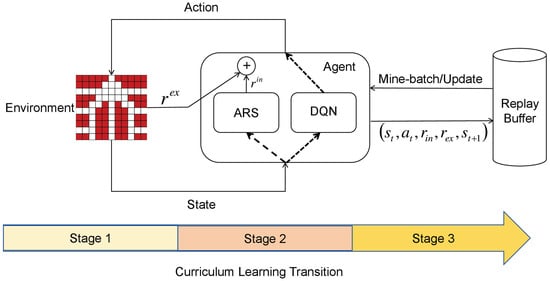
Figure 1. CLARS-DQN Framework.

Notation.

We use the following notation throughout.

• $\theta$: policy parameters;
• $\eta$: intrinsic reward parameters;
• $r^{ex}$: extrinsic reward;  
• $r^{in}$: intrinsic reward;  
• $r^{ex+in}$: the sum of extrinsic reward and intrinsic reward;  
• ${\xi }^i$: the ith trajectory; $\left(s_0^i,a_0^i,s_1^i,a_1^i,···,s_H^i\right)$;  
• ${\xi }_t^i$ = $\left(s_t^i,a_t^i,s_{t+1}^i,a_{t+1}^i,···,s_H^i\right)$;  
• $J^{ex}=E_{\theta }\left[{\sum }_{t=0}^{\infty }{\gamma }^t{r}_t^{ex}\right]$;  
• $G^{ex}\left(s_t,a_t\right)={\sum }_{i=t}^{\infty }{\gamma }^{i-t}{r}_i^{ex}$;  
• $G_h^{ex+in}\left(s_t,a_t\right)={\sum }_{i=t}^{t+h}{\gamma }^{i-t}{r}_i^{ex+in}$.

3.1. Adaptive Reward Shaping

The goal of adaptive reward shaping is to enable the agent to autonomously learn an appropriate intrinsic reward function during training, thereby providing additional guidance beyond the sparse extrinsic signals. The intrinsic reward function is implemented using a neural network. This method incorporates the concept of meta-learning, where the intrinsic reward function is continually adjusted to influence the agent’s policy learning, ultimately optimizing its performance on the actual task—maximizing cumulative extrinsic rewards. In practice, the parameters of the intrinsic reward function are updated by computing its meta-gradient with respect to the cumulative extrinsic reward, i.e.,

$${\eta }^{\prime }=\eta +\alpha ·{\nabla }_{\eta }{J}^{ex}.$$

(4)

In the LIRPG method, this meta-gradient is computed using the chain rule. The algorithm first computes the gradient of the policy with respect to the extrinsic reward, and then the gradient of the intrinsic reward with respect to the policy parameters [19], as follows:

$${\nabla }_{\eta }{J}^{ex}={\nabla }_{\theta }{J}^{ex}·{\nabla }_{\eta }\theta ,$$

(5)

where the first term $\left({\nabla }_{\theta }{J}^{ex}\right)$ can be sampled as:

$${\nabla }_{\theta }{J}^{ex}\approx G^{ex}\left(a_t,s_t\right)·{\nabla }_{\theta }log{\pi }_{\theta }\left(a_t|s_t\right),$$

(6)

according to the policy gradient theorem of Sutton et al. [21]. The second term $\left({\nabla }_{\eta }\theta \right)$ can be written as:

$${\nabla }_{\eta }\theta =\alpha {\nabla }_{\eta }{G}_h^{ex+in}·{\nabla }_{\theta }log{\pi }_{\theta }\left(a_t|s_t\right),$$

(7)

according to the meta-gradient derivations in [22,23,24], where $\alpha$ is the policy learning rate.

However, this method relies on policy gradients, which limits its applicability to policy-based reinforcement learning methods. For value-based methods such as Q-learning, it is not feasible to compute the gradient of the intrinsic reward with respect to the policy, since the actions are selected based on Q-values rather than a parameterized policy.

To address this limitation, we conduct a two-stage derivation. First, we follow [18] to derive the meta-gradient in value-based methods form (Equations (8)–(13)). Then, we extend this derivation by introducing softmax policy approximation, which enables the use of softmax to approximate $\epsilon -greedy$ policy while maintaining theoretical validity. This extension allows the method to be applied in settings where actions are selected using $\epsilon -greedy$ policy, with the softmax approximation used only for gradient computation during parameter updates.

$${\pi }_{\theta }\left(a|s\right)={\displaystyle \frac{exp\left(\theta \left(s,a\right)\right)}{{\sum }_{b\in A}exp\left(\theta \left(s,b\right)\right)}}.$$

(8)

To enable the application of ARS to value-based methods, we need to eliminate the dependency of policy gradients. This goal is achieved through softmax policy approximation. We assume that the policy can be represented in softmax form as in Equation (8), where $\theta \left(s,a\right)$ is the parameter for state action pair $\left(s,a\right)$.

Then we introduce a critic network to estimate the value of a given state s and define the advantage functions:

$$A_{r^{\mathrm{ex}+\mathrm{in}},h}^{{\pi }_k}(s,a)=Q_{r^{\mathrm{ex}+\mathrm{in}},h}^{{\pi }_k}(s,a)-V_{r^{\mathrm{ex}+\mathrm{in}},h}^{{\pi }_k}\left(s\right);$$

(9)

$$A_{r^{\mathrm{ex}}}^{{\pi }_k}(s,a;r^{\mathrm{ex}})=Q_{r^{\mathrm{ex}}}^{{\pi }_k}(s,a;r^{\mathrm{ex}})-V_{r^{\mathrm{ex}}}^{{\pi }_k}(s;r^{\mathrm{ex}}),$$

(10)

where:

$$V_{r^{\mathrm{ex}+\mathrm{in}},h}^{{\pi }_k}\left(s\right)=\sum _a{\pi }_k\left(a\right|s)Q_{r^{\mathrm{ex}+\mathrm{in}},h}^{{\pi }_k}(s,a);$$

(11)

$$V_{r^{\mathrm{ex}}}^{{\pi }_k}(s;r^{\mathrm{ex}})=\sum _a{\pi }_k\left(a\right|s)Q_{r^{\mathrm{ex}}}^{{\pi }_k}(s,a;r^{\mathrm{ex}}).$$

(12)

The gradient term in Equation (5) takes the following form:

$$\eta ·{\mathbb{E}}_{s\sim d^{{\pi }_k},a\sim {\pi }_k}\left[d^{{\pi }_k}(s,a)·A_r^{\pi }(s,a;r^{\mathrm{ex}})·\left[{\nabla }_{\eta }\left(r^{in}(s,a)-{\mathbb{E}}_{\pi \left(b\right|s)}\left[r^{in}(s,b)\right]\right)\right]\right],$$

(13)

where $d^{{\pi }_k}(s,a)=d^{{\pi }_k}\left(s\right)·{\pi }_k\left(a\right|s)$ is the state-action joint distribution.

This approach does not require computing policy gradients, making it applicable to any class of reinforcement learning algorithms, including value-based ones [18].

Softmax Policy Approximation in $ϵ$-Greedy Settings

A potential concern is the compatibility between the softmax policy approximation used for gradient computation and the $ϵ$-greedy action selection used during DQN training. We address this concern both theoretically and empirically by establishing a crucial distinction between two different stages of the learning process. In the action selection stage, where the agent interacts with the environment, we use the $ϵ$-greedy strategy to select actions. Specifically, with probability $(1-ϵ)$, the agent selects the greedy action $arg{max}_{a}Q(s,a)$, and with probability $ϵ$, it randomly selects an action. In contrast, during the gradient computation stage for parameter updates, we employ softmax policy approximation solely for computing meta-gradients. This softmax approximation is used exclusively for gradient computation and does not affect action selection during environment interaction.

The following theorem establishes the theoretical validity of softmax approximation under $ϵ$-greedy action selection. Let ${\pi }_{ϵ}\left(a\right|s)=(1-ϵ)·\mathbf{1}[a=arg{max}_{b}Q(s,b)]+ϵ/\left|A\right|$ denote the $ϵ$-greedy policy, and let ${\pi }_{\tau }\left(a\right|s)=exp(Q(s,a)/\tau )/{\sum }_{b}exp(Q(s,b)/\tau )$ denote the softmax policy used for gradient computation. We define the true gradient as $g_{\mathrm{true}}={\mathbb{E}}_{s\sim \rho ,a\sim {\pi }_{ϵ}}[{\nabla }_{\theta }log{\pi }_{\tau }\left(a\right|s)·R^{\mathrm{total}}]$ and the softmax approximation gradient as ${\widehat{g}}_{\mathrm{softmax}}={\mathbb{E}}_{s\sim \rho ,a\sim {\pi }_{\tau }}[{\nabla }_{\theta }log{\pi }_{\tau }\left(a\right|s)·R^{\mathrm{total}}]$.

When using $ϵ$-greedy action selection with exploration rate $ϵ>0$, the softmax policy approximation provides an effective gradient estimate for meta-gradient computation. Specifically, when the temperature parameter $\tau$ satisfies $\tau =O\left(ϵ\right)$, there exists a constant C such that the gradient estimation error is bounded by:

$$\parallel g_{\mathrm{true}}-{\widehat{g}}_{\mathrm{softmax}}\parallel \le C·ϵ.$$

(14)

The proof analyzes the gradient difference in two phases. In the exploitation phase, which occurs with probability $(1-ϵ)$, the $ϵ$-greedy policy selects $arg{max}_{a}Q(s,a)$. When $\tau \to 0$, the softmax policy also converges to $arg{max}_{a}Q(s,a)$, making the two policies consistent in this phase with zero error. In the exploration phase, which occurs with probability $ϵ$, the $ϵ$-greedy policy uniformly randomly selects actions, while the softmax policy still concentrates on high Q-value actions. The difference in this phase is bounded by $O(ϵ/|A\left|\right)$. The total error is therefore $(1-ϵ)·0+ϵ·O(1/|A\left|\right)=O\left(ϵ\right)$. The complete proof is provided in Appendix A.

In practice, we set $\tau =ϵ$. This ensures that in the exploitation phase, the softmax policy is consistent with the greedy component of the $ϵ$-greedy policy. In the exploration phase, the error remains bounded by $O\left(ϵ\right)$, and the total error is bounded and does not affect convergence. This practical implementation demonstrates that the softmax approximation can be effectively used for gradient computation while maintaining compatibility with $ϵ$-greedy action selection during training.

3.2. ARS-DQN

Building on the meta-gradient computation framework developed in Section 3.1, we integrate adaptive reward shaping with the DQN framework to develop ARS-DQN. During training, we update both the Q-network and the intrinsic reward function iteratively, forming a bi-level optimization problem. Specifically, the DQN update corresponds to the inner optimization, which aims to maximize the sum of the cumulative extrinsic and intrinsic rewards. In each training iteration, we first update the parameters of the Q-network. The loss function of Q-network is defined as:

$$L\left(\theta \right)={\displaystyle \frac{1}{N}}\sum _1^N{\left[r^{ex+in}+\gamma ·\underset{a_{t+1}\in A}{max}Q\left(s_{t+1},a_{t+1}|{\theta }^{-}\right)-Q\left(s_t,a_t|\theta \right)\right]}^2.$$

(15)

where ${\theta }^{-}$ is the parameters of target network. After updating the Q-network, we hold its parameters fixed and update the intrinsic reward function using the meta-gradient formulation described in Equation (13), based on the current Q-values. Simultaneously, a critic network is trained to estimate the value of states, and its loss function is defined as:

$$L\left({\theta }_v\right)=smoothL1\left(V\left(s_t\right),G^{ex}\left(s_t,a_t\right)\right).$$

(16)

The complete training process is illustrated in the pseudocode shown in Algorithm 1 from line 13 to line 22. To improve training efficiency, we adopt PER for sample selection within the DQN framework. PER assigns sampling probabilities based on the importance of each experience, ensuring that transitions with higher learning value are sampled more frequently. This enhances the agent’s ability to learn from critical experiences, improving convergence speed. Moreover, unlike on-policy methods used in [18,19], experience replay enables repeated use of the same transition samples, increasing sample efficiency and breaking the temporal correlations between consecutive samples. This leads to more stable and robust parameter updates during training.

3.3. Curriculum-Guided Training Strategy

Curriculum learning draws inspiration from the human learning process, whereby learners progress from simple to complex tasks. During training, the agent first interacts with and learns in a simple environment. Once it acquires a basic capability for policy learning, the complexity of the environment is gradually increased. This incremental strategy enables the agent to ultimately acquire the ability to perform path planning tasks in complex environments. In this study, we adopt a three-stage curriculum learning paradigm. In the first stage, the agent is trained in an environment without any obstacles. At this stage, the agent primarily learns how to find a path from the start to the goal without interference. In the second stage, a small number of regularly distributed and sparsely placed static obstacles are introduced into the environment. The policy obtained from the first stage is fine-tuned in this new environment, allowing the agent to acquire basic obstacle-avoidance capabilities. In the third stage, the environment is significantly more challenging, containing densely packed obstacles and predominantly narrow or curved paths. The final agent policy is obtained through training in this environment. Progression from one stage to the next is conditional on the agent achieving a predefined task success rate. In this work, we set the success threshold to 80%; once the agent’s success rate in the current stage exceeds this value, training proceeds to the next stage.

3.4. CLARS-DQN

Algorithm 1 presents the pseudocode of the CLARS-DQN algorithm. During initialization, we employ the convolutional neural network (CNN) with the same architecture for the Q-network, the intrinsic reward function network, and the critic network. These networks take the two-dimensional environmental state tensor as input. Both the Q-network and the intrinsic reward function output a one-dimensional vector whose length equals the size of the action space, representing the state-action values and the intrinsic reward values for each action, respectively. The critic network outputs a scalar that estimates the value of the input state. During training, to enhance stability, the intrinsic reward function is updated less frequently than the Q-network. Specifically, the Q-network is updated for multiple iterations before a single update is applied to the intrinsic reward network.

Algorithm 1 CLARS-DQN

1: Hyperparameters: PER buffer B with size $B_{max}$; extrinsic reward $r^{ex}$; learning rates $\left\{{\alpha }_{\theta },{\alpha }_{\eta }\right\}$; discount factor $\gamma$; update rates $\left\{N_r,N_{\pi },N_e\right\}$; evaluate metric S; threshold $S_{th}$; environment list = $\left[en{v}_1,en{v}_2,en{v}_3\right]$ 2: Initialization: Initialize the parameters for Q-network $\theta$, the intrinsic reward $\eta$ and its critic V 3: $stage=1$ 4: $env=en{v}_{stage}$ 5: for  $k=1,2,\dots ,K$  do 6:     if $kmod{N}_e=0$ then 7:         evaluate current training model using 100 random test case and calculate success rate S 8:         if $S>=S_{th}$ then 9:              $stage=stage+1$ 10:            $env\leftarrow en{v}_{stage}$ 11:       end if 12:     end if 13:     if $kmod{N}_{\pi }=0$ then 14:         sample transitions from buffer B 15:         update Q-network $\theta$ using sampled transitions as in Equation (15) 16:     end if 17:     RL agent interact with env to obtain a new trajectory ${\xi }^k$ 18:     Store ${\xi }^k$ in the buffer B 19:     if $kmod{N}_r=0$ then 20:         sample transitions from buffer B 21:         update intrinsic reward parameter $\eta$ using sampled transitions as in Equation (13) 22:         update critic parameter V using sampled transitions as in Equation (16) 23:     end if 24: end for 25: Output: Q-network ${\theta }_K$

In practice, we define two hyperparameters $N_Q$ and $N_R$ to control the number of update steps, where $N_R<N_Q$. After training, the parameters ${\theta }_k$ of the Q-network are used as the final decision-making policy for the agent.

4. Experimental Evaluation

The proposed algorithm and simulation environment were implemented using Python 3.10 and PyTorch 2.1.0, and all training was conducted on an Intel Xeon E5-2630v3 CPU. Following the design in [25], we constructed three types of map environments with increasing levels of complexity: the blank layout, the rectangular layout, and the fishbone layout. These maps vary in terms of obstacle quantity and spatial density, leading to progressively more challenging path planning tasks. In accordance with the curriculum learning framework, CLARS-DQN was trained sequentially on the three map types—from the simplest (blank) to the most complex (fishbone). In contrast, all baseline models were trained directly on the fishbone map without prior curriculum stages. To validate the effectiveness of CLARS-DQN, we compared it against standard DQN and several DRL algorithms incorporating different reward shaping strategies [2,10,13].

Baseline Models:

• IDDQN [13]: Based on DQN, IDDQN introduces a heuristic-driven reward term that ensures alignment between the reward function and the model’s optimization objectives, thereby improving the safety and efficiency of path planning.
• EPPE-DQN: The EPPE framework [2] dynamically adjusts the weights of multiple reward components and the learning rate during training to address reward entanglement in DRL. We integrate EPPE into the DQN architecture using the hyperparameter settings recommended in [2].
• Count-based DQN [10]: This method provides the agent with intrinsic rewards based on state visitation counts. Less frequently visited (i.e., more novel) states yield higher rewards, encouraging thorough exploration. We implement this strategy on top of DQN as a baseline.

All baseline models were configured with the same neural network architecture and hyperparameters as CLARS-DQN to ensure fair comparison and eliminate the influence of irrelevant factors. The hyperparameter settings used by CLARS-DQN are listed in Table 1. We evaluate model performance using two metrics: Success Rate (SR) and Average Path Length (APL). SR is defined as the number of successful task completions divided by the total number of tasks. APL is the total path length over all episodes divided by the number of tasks. For episodes where the agent fails to reach the target, the path length is counted as the maximum allowable episode length (Max Length per episode).

Table 1. Hyperparameter Settings.

Hyperparameter	Value
Learning rate (${\alpha }_{\theta },{\alpha }_{\eta }$)	0.001
Discount factor ($\gamma$)	0.97
Batch size	64
Replay buffer size	${10}^5$
Policy network update frequency ($N_{\pi }$)	20
Target network update frequency	100
Intrinsic reward update frequency ($N_{\eta }$)	100
Intrinsic reward weight coefficient	0.1
Max Length per episode	72
Map size	$25\times 25$

4.1. Experimental Results and Analysis

We first trained CLARS-DQN and all baseline models, and the resulting reward curves are shown in Figure 2. The x-axis represents the number of training episodes and the y-axis indicates the agent’s average cumulative reward.

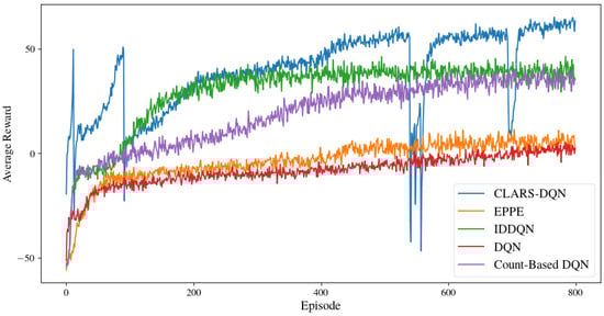
Figure 2. Average reward value of CLARS-DQN model and baseline models.

From the reward curves, it is evident that standard DQN performs poorly in environments with sparse rewards. All reward shaping methods demonstrate performance improvements over vanilla DQN, and the reward curves of the three baseline models exhibit similar trends. At the beginning of training, the agents’ policies are nearly random, resulting in large negative rewards. As training progresses, the agents gradually gain an initial understanding of the environment, leading to a rapid increase in cumulative reward during the early stages. After a temporary plateau, the cumulative rewards continue to rise and eventually converge near their respective maximum values.

However, after convergence, a significant performance gap emerges between CLARS-DQN and the baseline models. Among the baselines, EPPE-DQN performs the worst—only marginally better than vanilla DQN. This observation suggests that while manually designed reward shaping functions can enhance the training efficiency and final performance of DRL models, they may be susceptible to local optima. Additionally, their applicability across different task scenarios can be limited, as determining suitable reward weight coefficients often requires considerable manual tuning. In contrast, CLARS-DQN significantly outperforms all baselines in both training efficiency and final performance, converging to a solution close to the global optimum. These results highlight the effectiveness of CLARS-DQN in enhancing model performance and addressing the reward coupling problem inherent in traditional reward shaping methods.

To more comprehensively evaluate the performance of each model, we conducted tests in both the training environments and unseen environments. The results are shown in Table 2 and Table 3. Table 2 indicates that CLARS-DQN outperforms the baseline models in terms of both task success rate and average path length. Compared to the best-performing baseline, CLARS-DQN improves the task success rate and average path length by 2% and 7.4%, respectively. In addition, experimental results show that the single-step inference time of CLARS-DQN is comparable to that of the baseline models. For the design of the unseen environments, we followed the setup in [26] and created five maps that were not used during training: Chevron warehouse, Discrete cross aisle warehouse, Diagonal cross-aisle warehouse, Flying-V warehouse, and Leaf warehouse. We evaluated all models on these maps and reported the average performance metrics in Table 3. The results demonstrate that CLARS-DQN maintains strong performance in unseen environments, indicating better generalization capabilities compared to the baseline models. Specifically, it improves the task success rate and average path length by 12% and 26%, respectively, compared to the best-performing baseline.

Table 2. Performance of models on training environment.

Model	SR	APL
CLARS-DQN	0.99	21.30
IDDQN	0.97	22.88
Count-Based DQN	0.94	25.40
EPPE-DQN	0.64	38.44
DQN	0.59	41.46

Table 3. Performance of models on unseen environment.

Model	SR	APL
CLARS-DQN	0.98	23.96
IDDQN	0.86	30.20
Count-Based DQN	0.81	29.92
EPPE-DQN	0.47	47.00
DQN	0.24	59.66

When using the adaptive reward shaping method, the agent’s reward function includes a weight parameter w (see Equation (3)). To further evaluate the robustness of the adaptive reward shaping method with respect to hyperparameters, we trained ARS-DQN in the same simulation environment while adjusting the weight parameter of the adaptive reward term. We then observed how the model performed under different values of this parameter. For comparison, we used IDDQN (the best-performing baseline model) as a reference. The experimental results are shown in Figure 3.

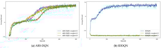
Figure 3. Average reward value of ARS-DQN and IDDQN under different weight coefficient.

We observed that for DQN with ARS, although the convergence speeds varied when the weight parameter was set to 0.1, 0.3, and 0.5, the maximum cumulative rewards achieved after convergence were similar across all three settings. In contrast, the IDDQN model exhibited significantly degraded performance when the reward weight was set to 0.3 or 0.5, indicating that compared to manually designed intrinsic rewards, the adaptive reward exhibits stronger robustness to the weight parameter. This suggests that it is easier to obtain a suitable weight value with lower manual tuning effort.

While a complete theoretical proof remains open, preliminary analysis suggests that ARS reduces reward coupling and achieves weight robustness through two interconnected mechanisms. First, the meta-learning process that optimizes intrinsic rewards to maximize extrinsic rewards implicitly normalizes the intrinsic reward scale to align with the extrinsic reward scale, reducing spatial and temporal coupling that arises from scale mismatch [18,19]. This implicit normalization mechanism, consistent with the optimal rewards framework [27], enables the learned intrinsic reward to automatically adjust its magnitude inversely to the weight parameter w, such that the product $w·R_{\eta }$ remains approximately stable across different w values. Second, the meta-gradient update uses advantage functions (relative differences) rather than absolute reward values, which reduces sensitivity to scale changes introduced by different w values, consistent with principles from potential-based reward shaping theory [28]. This relative structure, combined with the adaptive nature of learned intrinsic rewards, enables dynamic decoupling where the intrinsic reward can learn state- and time-dependent signals that automatically avoid conflicts with extrinsic rewards, unlike fixed manually-designed rewards. We hypothesize that these mechanisms collectively reduce reward coupling by enabling the intrinsic reward to adapt both spatially (across different states) and temporally (during training), thereby reducing the sensitivity of the total reward function to weight variations.

This hypothesis is supported by our observation that learned intrinsic rewards exhibit different magnitudes when trained with different w values, and is consistent with empirical robustness observations in related adaptive reward shaping methods [18]. Rigorous proofs remain challenging due to the complexity of meta-learning dynamics in bi-level optimization settings [29]. Future work should investigate formal characterization of these decoupling mechanisms and explore adaptive weight learning to eliminate manual tuning.

4.2. Computational Efficiency Analysis

This section analyzes the computational efficiency of ARS-DQN compared to standard DQN and other baseline methods, focusing on training time and memory overhead.

4.2.1. Training Time Analysis

To evaluate the computational efficiency, we measured the training time per 100 episodes for ARS-DQN and baseline methods on the same hardware configuration. Table 4 shows the training time comparison.

Table 4. Training Time Comparison: Time per 100 Episodes.

Method	Time per 100 Episodes (s)
DQN	8.83
IDDQN	8.96
EPPE-DQN	9.17
Count-Based DQN	9.40
ARS-DQN	11.04

ARS-DQN requires 11.04 s per 100 episodes compared to 8.83 s for standard DQN. This represents a 25.0% overhead per 100 episodes. This overhead is higher than other baseline methods (IDDQN: 1.5%, EPPE-DQN: 3.8%, Count-Based DQN: 6.5%), which is expected as ARS-DQN introduces additional components for adaptive reward learning.

ARS-DQN time breakdown: To better understand the time overhead, we analyzed the time breakdown of ARS-DQN per 100 episodes. Table 5 shows that the ARS-specific components account for 1.99 s (18.0% of total time) per 100 episodes, while the DQN base components account for 0.54 s (4.9% of total time). The majority of training time (77.1%, 8.51 s) is spent on other operations such as environment interaction, experience replay sampling, and data processing.

Table 5. ARS-DQN Training Time Breakdown per 100 Episodes.

Component	Time per 100 Episodes (s)	Percentage (%)
DQN base operations	0.54	4.9
ARS additional operations	1.99	18.0
Other operations	8.51	77.1
Total ARS-DQN	11.04	100.0
Standard DQN	8.83	-
Additional Overhead	2.21	25.0

The 18.0% time overhead from ARS-specific components per 100 episodes is acceptable because:

• The absolute additional time per 100 episodes (2.21 s) is minimal in practice.
• Although the per-episode overhead is 25.0%, ARS-DQN achieves faster convergence (see Section 4.1), potentially requiring fewer total episodes to reach the target performance, which may offset the per-episode overhead.
• The performance benefits demonstrated in Section 4.1 justify this modest overhead.

4.2.2. Memory Overhead Analysis

Table 6 shows the memory usage for network parameters in DQN and ARS-DQN.

Table 6. Memory Usage Comparison: Network Parameters.

Network Component	DQN (MB)	ARS-DQN (MB)
Q-network	9.61	9.61
Target network	9.61	9.61
Intrinsic reward network	-	9.61
Critic network	-	9.60
Total Network Parameters	19.22	38.43
Additional Parameters (ARS-DQN)	-	19.21
Memory Overhead	-	100.0%

ARS-DQN requires 38.43 MB for network parameters compared to 19.22 MB for standard DQN, representing a 100.0% overhead (doubling the parameter memory). The additional 19.21 MB is used for the intrinsic reward network (9.61 MB) and critic network (9.60 MB).

4.2.3. Efficiency Trade-Offs

The efficiency trade-off is favorable: a 25.0% per-episode time overhead and 100.0% parameter memory overhead (but only 4% of total memory) result in substantial performance improvements. The absolute overhead per 100 episodes (2.21 s) and additional memory (19.21 MB) are negligible in practice, making ARS-DQN practical for real-world path planning applications.

4.3. Ablation Study

To evaluate the contribution of each component in CLARS-DQN, we conducted ablation studies, and the results are shown in Figure 4.

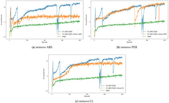
Figure 4. Ablation study: Results when removing module ARS, PER, and CL, respectively.

As illustrated in Figure 4a, the ARS module has the most significant impact on the model’s final performance. With the ARS module, training efficiency is greatly improved, and the cumulative reward obtained after convergence is notably higher than that of the model without ARS. This demonstrates the critical role of ARS in guiding policy iteration and helping the agent acquire near-optimal policies. Comparing the reward curves in Figure 4b, we observe that the inclusion of the PER module has minimal effect on the model’s final performance after convergence. However, at each stage of curriculum learning, models with the PER module achieve faster cumulative reward growth, indicating that PER positively contributes to training efficiency by prioritizing the selection of more informative samples and enabling the model to optimize its policy more rapidly. As shown in Figure 4c, models that include the CL module exhibit improvements in both training efficiency and performance. The reward curves converge more quickly, and the final cumulative rewards are higher compared to models without CL. We also evaluated the generalization ability of the ablation models in unseen environments, as shown in Table 7. The results indicate that both ARS and CL significantly enhance the model’s generalization performance. Among them, ARS plays a decisive role in improving the model’s final performance. During training, the PER module improves training efficiency and contributes modestly to enhancing generalization capability.

Table 7. Performance of models in ablation experiments.

Model	SR	APL
CLARS-DQN	0.98	23.96
without ARS	0.59	41.62
without CL	0.79	33.24
without PER	0.91	26.46

5. Conclusions

To address the challenge of path planning in sparse reward environments, this paper proposes the CLARS-DQN algorithm. First, to overcome the issues of reward coupling and the difficulty of manually tuning reward shaping functions, the algorithm integrates adaptive reward shaping with the DQN framework. Second, to further enhance training efficiency and generalization ability, we employ a curriculum learning strategy to train the DRL model and incorporate the PER method during training. Experimental results demonstrate that the proposed approach achieves superior performance in terms of generalization capability, sample efficiency, and path quality. Moreover, the method exhibits strong robustness to the weighting parameter of the intrinsic reward term, significantly simplifying the hyperparameter tuning process. In future work, we plan to extend our method to environments with continuous action spaces and dynamic changes, as well as to explore its application in multi-agent scenarios.

References

- Wang, B.; Liu, Z.; Li, Q.; Prorok, A. Mobile robot path planning in dynamic environments through globally guided reinforcement learning. IEEE Robot. Autom. Lett. 2020, 5, 6932–6939. [Google Scholar] [CrossRef]
- Zhao, W.; Zhang, Y.; Xie, Z. EPPE: An Efficient Progressive Policy Enhancement framework of deep reinforcement learning in path planning. Neurocomputing 2024, 596, 127958. [Google Scholar] [CrossRef]
- Li, X.; Liang, X.; Wang, X.; Wang, R.; Shu, L.; Xu, W. Deep reinforcement learning for optimal rescue path planning in uncertain and complex urban pluvial flood scenarios. Appl. Soft Comput. 2023, 144, 110543. [Google Scholar] [CrossRef]
- Lin, X.; McConnell, J.; Englot, B. Robust unmanned surface vehicle navigation with distributional reinforcement learning. In Proceedings of the 2023 IEEE/RSJ International Conference on Intelligent Robots and Systems (IROS), Detroit, MI, USA, 1–5 October 2023; pp. 6185–6191. [Google Scholar]
- Angulo, B.; Panov, A.; Yakovlev, K. Policy optimization to learn adaptive motion primitives in path planning with dynamic obstacles. IEEE Robot. Autom. Lett. 2022, 8, 824–831. [Google Scholar] [CrossRef]
- Zheng, S.; Liu, H. Improved multi-agent deep deterministic policy gradient for path planning-based crowd simulation. IEEE Access 2019, 7, 147755–147770. [Google Scholar] [CrossRef]
- Ang, W.; Bai, C.; Cai, C.; Zhao, Y.; Liu, P. Survey on sparse reward in deep reinforcement learning. Comput. Sci. 2020, 47, 182–191. [Google Scholar]
- Ibrahim, S.; Mostafa, M.; Jnadi, A.; Salloum, H.; Osinenko, P. Comprehensive overview of reward engineering and shaping in advancing reinforcement learning applications. IEEE Access 2024, 12, 175473–175500. [Google Scholar] [CrossRef]
- Shi, H.; Shi, L.; Xu, M.; Hwang, K.S. End-to-end navigation strategy with deep reinforcement learning for mobile robots. IEEE Trans. Ind. Inform. 2019, 16, 2393–2402. [Google Scholar] [CrossRef]
- Tang, H.; Houthooft, R.; Foote, D.; Stooke, A.; Chen, X.; Duan, Y.; Schulman, J.; DeTurck, F.; Abbeel, P. #Exploration: A study of count-based exploration for deep reinforcement learning. In Proceedings of the Advances in Neural Information Processing Systems 30 (NeurIPS), Long Beach, CA, USA, 4–9 December 2017. [Google Scholar]
- Burda, Y.; Edwards, H.; Storkey, A.; Klimov, O. Exploration by random network distillation. arXiv 2018, arXiv:1810.12894. [Google Scholar] [CrossRef]
- Yan, C.; Chen, G.; Li, Y.; Sun, F.; Wu, Y. Immune deep reinforcement learning-based path planning for mobile robot in unknown environment. Appl. Soft Comput. 2023, 145, 110601. [Google Scholar] [CrossRef]
- Bai, Z.; Pang, H.; He, Z.; Zhao, B.; Wang, T. Path planning of autonomous mobile robot in comprehensive unknown environment using deep reinforcement learning. IEEE Internet Things J. 2024, 11, 22153–22166. [Google Scholar] [CrossRef]
- Wu, C.; Yu, W.; Li, G.; Liao, W. Deep reinforcement learning with dynamic window approach based collision avoidance path planning for maritime autonomous surface ships. Ocean Eng. 2023, 284, 115208. [Google Scholar] [CrossRef]
- Zhang, C.; Vinyals, O.; Munos, R.; Bengio, S. A study on overfitting in deep reinforcement learning. arXiv 2018, arXiv:1804.06893. [Google Scholar] [CrossRef]
- Hafiz, A.M. A survey of deep q-networks used for reinforcement learning: State of the art. In Intelligent Communication Technologies and Virtual Mobile Networks: Proceedings of ICICV 2022, Tirunelveli, India, 10–11 February 2022; Springer: Singapore, 2022; pp. 393–402. [Google Scholar]
- Cederle, M.; Fabris, M.; Susto, G.A. A Distributed Approach to Autonomous Intersection Management via Multi-Agent Reinforcement Learning. In Proceedings of the 27th European Conference on Artificial Intelligence, Santiago de Compostela, Spain, 19–24 October 2024. [Google Scholar]
- Devidze, R.; Kamalaruban, P.; Singla, A. Exploration-guided reward shaping for reinforcement learning under sparse rewards. Adv. Neural Inf. Process. Syst. 2022, 35, 5829–5842. [Google Scholar]
- Zheng, Z.; Oh, J.; Singh, S. On learning intrinsic rewards for policy gradient methods. In Proceedings of the Advances in Neural Information Processing Systems 31, Montréal, QC, Canada, 3–8 December 2018. [Google Scholar]
- Yin, Y.; Chen, Z.; Liu, G.; Yin, J.; Guo, J. Autonomous navigation of mobile robots in unknown environments using off-policy reinforcement learning with curriculum learning. Expert Syst. Appl. 2024, 247, 123202. [Google Scholar] [CrossRef]
- Sutton, R.S.; McAllester, D.; Singh, S.; Mansour, Y. Policy gradient methods for reinforcement learning with function approximation. In Proceedings of the Advances in Neural Information Processing Systems 12, Denver, CO, USA, 29 November–4 December 1999. [Google Scholar]
- Andrychowicz, M.; Denil, M.; Gomez, S.; Hoffman, M.W.; Pfau, D.; Schaul, T.; Shillingford, B.; De Freitas, N. Learning to Learn by Gradient Descent by Gradient Descent. In Proceedings of the Advances in Neural Information Processing Systems, Barcelona, Spain, 5–10 December 2016. [Google Scholar]
- Santoro, A.; Bartunov, S.; Botvinick, M.; Wierstra, D.; Lillicrap, T. Meta-Learning with Memory-Augmented Neural Networks. In Proceedings of the International Conference on Machine Learning, New York, NY, USA, 20–22 June 2016. [Google Scholar]
- Nichol, A.; Achiam, J.; Schulman, J. On First-Order Meta-Learning Algorithms. arXiv 2018, arXiv:1803.02999. [Google Scholar]
- Luo, L.; Zhao, N.; Zhu, Y.; Sun, Y. A* guiding DQN algorithm for automated guided vehicle pathfinding problem of robotic mobile fulfillment systems. Comput. Ind. Eng. 2023, 178, 109112. [Google Scholar] [CrossRef]
- Masae, M.; Glock, C.H.; Vichitkunakorn, P. A method for efficiently routing order pickers in the leaf warehouse. Int. J. Prod. Econ. 2021, 234, 108069. [Google Scholar] [CrossRef]
- Singh, S.; Lewis, R.L.; Barto, A.G.; Sorg, J. Intrinsically motivated reinforcement learning: An evolutionary perspective. IEEE Trans. Auton. Ment. Dev. 2010, 2, 70–82. [Google Scholar] [CrossRef]
- Ng, A.Y.; Harada, D.; Russell, S. Policy invariance under reward transformations: Theory and application to reward shaping. In Proceedings of the International Conference on Machine Learning, Bled, Slovenia, 27–30 June 1999; Volume 99, pp. 278–287. [Google Scholar]
- Franceschi, L.; Frasconi, P.; Salzo, S.; Grazzi, R.; Pontil, M. Bilevel programming for hyperparameter optimization and meta-learning. In Proceedings of the International Conference on Machine Learning, PMLR, Stockholm, Sweden, 10–15 July 2018; pp. 1568–1577. [Google Scholar]
Disclaimer/Publisher’s Note: The statements, opinions and data contained in all publications are solely those of the individual author(s) and contributor(s) and not of MDPI and/or the editor(s). MDPI and/or the editor(s) disclaim responsibility for any injury to people or property resulting from any ideas, methods, instructions or products referred to in the content. |
© 2026 by the authors. Licensee MDPI, Basel, Switzerland. This article is an open access article distributed under the terms and conditions of the Creative Commons Attribution (CC BY) license.