Tradeoff Between Speed and Memory Requirements for Decoding of Prefix-Free Codes

Abstract

For the decoding of prefix-free codes such as Huffman code, we present a tradeoff between the decoding speed and memory requirements that results in an adapted decoding algorithm. Our decoding experiments on different codes demonstrate that the Pareto front of non-dominated solutions from different parameters comprises known solutions and solutions from our adapted algorithm. Each Pareto front comprises five solutions from our adapted algorithm next to five known solutions with a single table and one known solution with all possible tables. Compared to the fastest known solution with all possible tables, our adapted algorithm can achieve only 3.8% runtime overhead with only 66% of the memory requirements. Compared to a known solution with only one table, our adapted algorithm achieves up to 10% runtime improvement with three tables instead of one table. We conclude that our algorithm gives developers more and better choices to balance decoding speed and memory requirements.

1. Introduction

Prefix-free codes such as Huffman code are often used in source encoding [1]. Hence, efficient decoding algorithms of such codes are important. Recent developments have focused on decoding multiple chunks of long encoded strings in parallel, cf. e.g., [2]. For the sequential decoding of one chunk, the classic method is to repeatedly follow the path in the code tree until a symbol on a leaf is reached [3]. More efficient methods use a decoding table, yet provision of a single table with a u-bit index is seldom mentioned (we found it in a German textbook [4]), possibly because it only leads to an average progress per table lookup of $u-\overline{\delta }$, where $\overline{\delta }$ is the average length of an incomplete codeword at the end of the u bits and implies varying shift widths. We will refer to this method as one-table method below. Choueka et al. [5] and Sieminski [6] presented a method where for each possible incomplete codeword, a separate table is provided that decodes a u-bit string preceded by this incomplete codeword, achieving a progress of u bits per table lookup at the price of multiple tables, i.e., increased memory consumption. We will refer to this method as the all-table method below.

Especially in embedded systems, memory requirements are still a design constraint similar to processing speed. For example, video and audio decoding for mobile devices provides a challenge with respect to computational effort, which is related to energy consumption [7], and with respect to memory requirements [8]. Hence, we are investigating the tradeoff between decoding speed and memory requirements and adapt the all-table method by not providing all possible tables but only the ones that are mostly accessed in order to reduce memory requirements with the minimum reduction in decoding speed. We refer to this method as some-table method (with a parameter specifying the target number of tables) below. We give two heuristics to find the best selection of tables for a given code and a target number of tables, where the complex heuristic is based on a Markov chain analysis.

In experiments, we construct the Pareto front (using decoding speed and memory requirements for tables as the two dimensions to be minimized simultaneously) of non-dominated solutions from the one-table method, the all-table method, and the some-table method for different values of u and different target numbers of tables in the case of the some-table method. We can demonstrate for different codes that the Pareto front comprises solutions both from known approaches (one-table and all-table methods) and from our some-table method, thus giving developers more and better choices to choose a decoding algorithm with the best memory requirement for a given decoding speed or with the best decoding speed for a given memory requirement.

Hence, the contributions of our present research can be summarized as follows.

• We present a new algorithm (some-table method) where the number of decoding tables can be configured between the minimum (one-table method) and maximum (all-table method) memory consumption.
• We present two heuristics for how to select a targeted number of tables from the all-table method for maximizing decoding speed.
• We provide an implementation of all three methods and conduct experiments. For each value of the parameter u, the number of bits used for a table-lookup, we demonstrate that the different numbers of tables provide a tradeoff between memory consumption and decoding speed, thus increasing the possible options for application developers.
• While previous experiments focused on a particular value of the parameter u, we perform experiments for a range of values of the parameter u and construct a Pareto front of non-dominated solutions that optimize decoding speed and table memory requirements. The presence of the some-table method in the Pareto front that mostly replaces the all-table method illustrates that the some-table methods indeed provide additional optimal design choices for application developers that did not exist previously.

The remainder of this article is structured as follows. Section 2 introduces notations and algorithms from previous work that we will base our proposal on. In Section 3, we present our proposal that uses multiple tables, yet not all possible tables, as in previous work, together with an analysis and information on how to find the best selection of tables. Section 4 reports on the results of our experiments, while Section 5 discusses related work. Section 6 provides a conclusion and gives an outlook on future work.

2. Background

2.1. Notations

For a binary string $x\in {\{0,1\}}^{*}$, we denote the length of the string by $\left|x\right|$, and we denote the concatenation of two strings x and y by $xy$ or—for accentuation—by $x|y$. The unique binary string with length 0, the empty word, is denoted by $\epsilon$, with $\epsilon |x=x|\epsilon =x$ for any binary string $x\in {\{0,1\}}^{*}$.

For a binary string $x=x_0\cdots x_{n-1}$, a string $x^{\prime }$ is called a prefix of x if $x^{\prime }=x_0\cdots x_{k-1}$ for some $k\in \{0,1,\dots ,n\}$, denoted by $x^{\prime }=pr{f}_k\left(x\right)$. If $k<n$, $x^{\prime }$ is called a proper prefix. This means that $\epsilon$ is a proper prefix of any non-empty binary string x, while a string $x^{\prime }=x$ is a prefix, but not a proper prefix, of itself. The rest of the string without the prefix is called the suffix (of length $n-k$) and denoted by $su{f}_{n-k}\left(x\right)$ or, if the length $\left|x\right|$ is not explicitly mentioned, by $su{f}_{-k}\left(x\right)$.

A binary string x of length $u=\left|x\right|\ge 1$ can be interpreted as an integer in the range 0 to $2^u-1$. We will denote this integer by $i=⟨x⟩$. Inversely, each integer i in the range 0 to $2^u-1$ can be represented by a binary string x of length u. We will denote this binary string by $x=bi{n}_u\left(i\right)$.

2.2. Prefix-Free Codes and Decodable Strings

Let $\mathrm{\Sigma }$ be a finite source (or symbol) alphabet and $c:\mathrm{\Sigma }\to {\{0,1\}}^{*}$ a binary code. We consider prefix-free codes, i.e., codes where no codeword is a prefix of another codeword [1]. Such codes are normally described by a code tree, i.e., a binary tree with $\left|\mathrm{\Sigma }\right|$ leaves that are marked with the symbols, and where all edges are marked with 0 or 1 so that the sequence of marks along the unique path from tree root to any leaf corresponds to the codeword of the symbol on that leaf.

For a symbol sequence $s_0,\dots ,s_{n-1}$ with $s_i\in \mathrm{\Sigma }$ and a string $\Delta \in {\{0,1\}}^{*}$ that is a proper prefix of some codeword $c\left(s\right)$, the binary string

$$y:=y(s_0,\dots ,s_{n-1},\Delta )=c\left(s_0\right)\cdots c\left(s_{n-1}\right)\Delta \in {\{0,1\}}^{*}$$

(1)

can be decoded uniquely into

$$dec\left(y\right)=n,s_0,\dots ,s_{n-1},\Delta .$$

An arbitrary binary string $y\in {\{0,1\}}^{*}$ is of the form in Equation (1) so that it can be decoded. For strings y that are not of this form, we extend the function $dec$ via $dec\left(y\right)=-1,\epsilon$ to denote undecodable strings. For a general prefix-free code c, such undecodable strings can occur. An example of such an undecodable string is $y=0100$ for a symbol alphabet $\mathrm{\Sigma }=\{A,B\}$ and a code $c\left(A\right)=01$, $c\left(B\right)=11$. There is no possibility to partition y into the form of Equation (1) as 00 is neither a codeword nor the prefix of a codeword. For a Huffman code c and any other prefix-free code where the inner nodes of the code tree always have two children, every binary string y is of the form in Equation (1), cf. Lemma 1 in [9], so that we consider undecodable binary strings only optionally.

2.3. Decoding by Tree Traversal and Table Lookup

Assume a binary string x, which is a sequence of codewords as the encoding result of a prefix-free code, which is now to be decoded. We have observed that decoding is treated in far fewer textbooks than code construction or encoding, although decoding is more frequent than construction and encoding for transmission with stable symbol distribution or data compression [1]. The straightforward decoding starts at the root of the Huffman tree and follows the edge marked with the value of the next bit of the string, until it reaches a leaf. Then a symbol is decoded and can be output, while the decoding starts again at the root. Yet, for each bit of x, an access to a tree node and following an edge is needed.

Faster decoding algorithms use a precomputed table with $2^u$ entries and strive to decode u bits of binary string x at once. While acceleration through a table to us seems straightforward, we found this method only mentioned (as standard acceleration method) in one textbook in the German language [4]. The pre-computation consists of generating a table $D^u$ with $D^u\left[⟨x⟩\right]=dec\left(x\right)$ for each u-bit binary string x. This means that each possible string of u bits is decoded via pa re-computed function $dec$ as far as possible. A consequence is that u must be as least as large as the longest codeword, as this codeword must be decoded in one table access:

$$u\ge u_{min}=\underset{s\in \mathrm{\Sigma }}{max}\left|c\left(s\right)\right|.$$

(2)

The pseudo-code for the pre-computation is shown in Algorithm 1.

Algorithm 1: Pre-computation of table $D^u$ with $2^u$ entries, indexed with $u\ge u_{min}$ bits from codeword sequence encoded by given prefix-free code c with code tree $(T,r)$, where each entry consists of a list of symbols that can be decoded from u-bit index, plus the number of bits at the end of the index that cannot be decoded completely.

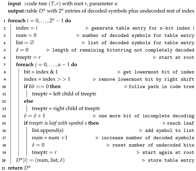The formulation of the precomputation is a simplification compared to the definition of the function $dec$, which not only stores the number of bits that cannot be completely decoded but even stores those bits themselves. We omitted this as it is not needed here and the extension is straightforward (cf. Section 2.4).

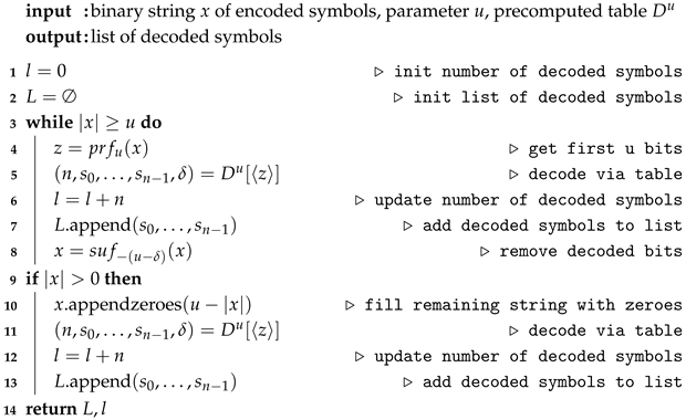
To decode a binary string x with encoded symbols, we can use u bits as the index into the table, receiving again the decoded symbols from this table entry together with the number $\delta$ of bits that could not be decoded completely (cf. Algorithm 1), and shifting x by $u-\delta$ bits. This is repeated until fewer than u bits are left of x. They are artificially expanded by bits with a value 0 to obtain u bits for a final decoding step. The pseudo-code of the one-table method is shown in Algorithm 2.

Line 8 in Algorithm 2 seems to assume that we can shift arbitrarily long bit sequences. However, as bit strings are often stored as sequences of bytes, with eight bits of the string in each byte, it is helpful if the start of the string is held in a window, i.e., a register variable of fixed length, so that shifts will only affect this variable. If the window runs empty, it gets refilled from the remaining bit string with one or more of the following bytes. In this case, lines 4 and 10 will also work on the window variable and not on the bit string x itself.

The space for the table is $u+2$ bytes per table entry (cf. line 5 in Algorithm 2): at most u symbols can be decoded if there is a codeword of 1 bit length, and each symbol index $s_i$ needs 1 byte if we consider the source symbol alphabets of size at most 256. Next to the sequence of the identifiers of decoded symbols, the number n of decoded symbols and the number $\delta$ of bits of the incompletely decoded rest are stored. As there is one table of $2^u$ entries, the space complexity of the one-table method is

$$m_{one}\left(u\right)=2^u(u+2)\mathrm{bytes}.$$

(3)

The time complexity of the decoding (we skip the pre-computation as it is only performed once) is determined by the number of iterations of the loop in lines 3 to 8 of Algorithm 2. The number of loops is

$$t_{one}\left(u\right)=O\left({\displaystyle \frac{\left|x\right|}{u-\overline{\delta }}}\right),$$

(4)

where $\overline{\delta }$ is the average value of $\delta$ as the progress is $u-\delta$ bits per loop. For a fixed input length $\left|x\right|$, the time is largely dependent on u. If u is notably larger than the maximum codeword length, $u-\overline{\delta }$ will approach u as $\delta$ is always smaller than a codeword length, and for longer bit sequences, there are more and more possibilities that the codeword lengths add up to u or $u-1$, so $\overline{\delta }$ will become smaller with larger u. The values of $\delta$ will depend on the particular code used. For example, a code with codewords 0, 10, 110, 111 resulting from symbols appearing with frequencies $2^{-1},2^{-2},2^{-3},2^{-3}$ will lead to encoded strings where 0 and 1 appear with equal frequency and also identical bi-gram frequencies for all bit-pair possibilities. In this case, the minimum $u=\left|\mathrm{\Sigma }\right|-1=3$. The corresponding decoding table is shown in Table 1. While it seems that one can compute $\overline{\delta }$ via $0·5/8+1·2/8+2·1/8=1/2$ as each entry has the same probability from the above argument, the situation is actually more complex. If $\delta =2$ in the case of 011, then the next index will be either 110 or 111, and the next $\delta$ will be 0. As the $\delta$ in each step only depends on the previous one, a simple Markov chain can be employed, which results in $\overline{\delta }=2/5$.

Table 1. Decoding table for example code and $u=3$. For illustration, the incompletely decoded rest $\Delta$ is also indicated.

Index	No. Decoded Symbols	Decoded Symbols	$\mathit{\delta }$/$\mathbf{\Delta }$
000	3	$s_0,s_0,s_0$	0/$\epsilon$
001	2	$s_0,s_0$	1/1
010	2	$s_0,s_1$	0/$\epsilon$
011	1	$s_0$	2/11
100	2	$s_1,s_0$	0/$\epsilon$
101	1	$s_1$	1/1
110	1	$s_2$	0/$\epsilon$
111	1	$s_3$	0/$\epsilon$

Algorithm 2: Decoding of binary string x that is encoded by code c, using precomputed table $D^u$.

2.4. Variant with Many Tables

In the previous code, the progress in a step is only $u-\overline{\delta }$ bits because some bits at the end of a u-bit piece cannot be completely decoded, and $\overline{\delta }$ is the average of this number given the symbol distribution.

Choueka et al. [5] and Sieminski [6] independently proposed a variant that can proceed by u bits in each step. The price is a larger number of tables. During the precomputation, for each possible prefix $\pi$ of a codeword, a table $D_{\pi }^u$ is generated via $D_{\pi }^u\left[i\right]=dec\left(\pi \right|bi{n}_u\left(i\right))$ for each $i=0,1,\dots ,2^u-1$, alternatively put as $D_{\pi }^u\left[⟨x⟩\right]=dec\left(\pi \right|x)$ for each u-bit binary string x. Now the decoding of a long codeword can be postponed from one step, where the prefix of this codeword is the incomplete rest $\Delta$, to the next step, where this rest becomes the context $\pi =\Delta$ of that next decoding step. As a consequence, u can be smaller than the maximum codeword length, which might make up for the storage increase through the multiple tables. The pseudo-code for generating table $D_{\pi }^u$ is a generalization of the pseudo-code for the table $D^u=D_{\epsilon }^u$, which only needs to be modified in few places:

• Line 2 in Algorithm 1 now reads
  index = $\pi \left|\right(i<<\left|\pi \right|)$
  as the prefix $\pi$ is set into the lowermost bits of the index, and the normal index (the binary representation of i) is put in the next bits.
• Line 7 of Algorithm 1 now reads
  foreach  $j=0,\dots ,u+\left|\pi \right|-1$  do
  as also the bits of the context $\pi$ are to be considered for decoding.

Instead of table entries only storing the number of bits that are not completely decoded, those bits are additionally stored directly as per the definition of the function $dec$. This is achieved by using a second index variable that is only shifted by $\delta$ bits when a leaf is reached. Then, the content of this variable can be stored in line 20 of Algorithm 1.

Then, if some incompletely decoded bits remain at the end of one decoding step of a binary string x, those bits serve to select the table that is used in the next decoding step. The pseudo-code for the all-table decoding is shown in Algorithm 3.

We observe that not all prefixes of all codewords (corresponding to inner nodes of the code tree) might occur in practice, so some tables might never be used. If, for instance, a code produces only codewords of lengths 2 and 4 and $u=8$, then only the two-bit prefixes of four-bit codewords could appear, but one-bit and three-bit prefixes cannot. The realistic maximum set $S_{max}$ can be found iteratively during the pre-computation itself. Start with $S_{max}=\left\{\epsilon \right\}$. When $D_{\epsilon }^u$ is computed, you obtain an initial set of incomplete codewords from all values of $\Delta$ occurring in that table, which are added to the set S. When computing the corresponding tables for these values, some more values $\Delta$ might occur in these tables for which no table has been computed yet. These are also added to the set S and the corresponding tables are computed again. This loop continues until no further value $\Delta$ is found, for which no table has been computed yet.

Algorithm 3: Decoding of binary string x that is encoded by code c using precomputed tables $D_{\pi }^u$ for each possible proper prefix $\pi$ of each codeword in code c.

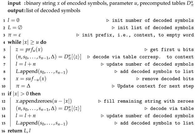The space requirements here are $u+3$ bytes per table entry (cf. line 6 in Algorithm 3): $u+1$ bytes for the decoded symbols and their number, and two bytes to represent $\Delta$ and $\delta =|\Delta |$. Each table has $2^u$ entries, and there is a table for each possible prefix, i.e., for each inner node of the code tree, of which there exist $|S_{max}|$. Thus, the space complexity of the all-table method is

$$m_{all}\left(u\right)=\left|S_{max}\right|·2^u(u+3)\mathrm{bytes}.$$

(5)

The time complexity is

$$t_{all}\left(u\right)=O\left({\displaystyle \frac{\left|x\right|}{u}}\right),$$

(6)

as the progress per iteration is u bits. The constant in the O-notation is similar to that of the one-table method, compare lines 4 to 8 in Algorithm 2 and lines 5 to 10 in Algorithm 3.

For the same value of u, the all-table method is faster than the one-table method for the price of a higher table space requirement. Yet, within limits, the user is free to choose u. From Equations (3) and (5), we see that the space requirements of the all-table method with parameter u will roughly correspond to the space requirements of the one-table method with parameter $u+{\log }_2\left(\right|S_{max}\left|\right)-1$. Hence, as long as $\overline{\delta }$ for the one-table method is smaller than ${\log }_2\left(\right|S_{max}\left|\right)-1$, the one-table method is faster than the all-table method with similar table space requirements.

3. Decoding with Some Tables

3.1. Proposed Algorithm

Some of the tables in the all-table method might only be needed rarely, so we propose a mix between the two systems: the some-table method that uses more than only table $D_{\epsilon }^u$ of the one-table method, yet fewer tables than the complete set $S_{max}$ of the all-table method.

Let $S\subset {\{0,1\}}^{*}$ be a finite set of binary strings that at least comprises the empty string $\epsilon$. In a pre-processing stage that resembles the pre-processing in the all-table, we compute tables $D_{\pi }^u$ for each $\pi \in S$. The choice of S and the choice of u will influence the runtime of the decoding algorithm below and will be subject to constraints to guarantee correctness of the decoding algorithm (cf. Section 3.2).

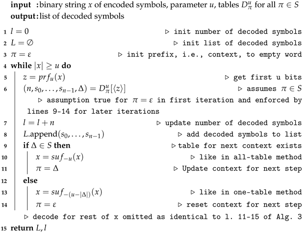
Our decoding algorithm strives to decode u bits of binary string x once in most of the steps: if an incompletely decoded rest $\Delta$ has one step, that becomes the context $\pi =\Delta$ of the next step, in S; then, the next step works as in the all-table method. Yet, if $\pi \notin S$, then x can only be shifted by $u-|\Delta |$ bits as in the one-table method from Section 2.3 and the next step accesses $D_{\epsilon }^u$. The pseudo-code of the some-table method is shown in Algorithm 4.

Algorithm 4: Decoding of binary string x that is encoded by code c using precomputed tables $D_{\pi }^u$ for each prefix $\pi \in S$.

3.2. Analysis

The correctness of Algorithm 4 immediately follows from the explanation in the previous section, as long as $u\ge u_{min}$, because then at least one symbol can be decoded in each execution of the WHILE loop.

The speed (for fixed u) follows from the possible choices of S. A minimum variant corresponds to the one-table method of Section 2.3 and uses $S_{min}=\left\{\epsilon \right\}$. In that case, any incomplete codeword at the end of a u-bit string, i.e., $\Delta \ne \epsilon$ in the result from the table lookup in line 6 will not be in S. Consequently, the condition in the IF statement (line 9) will be false, so that the incomplete codeword is not removed from the rest of the string to be decoded (line 13). This reduces the progress per iteration to the average number of bits for complete symbols in a u-bit string, which equals $u-\overline{\delta }$, where $\overline{\delta }$ is the average over the lengths $\delta$ in the table entries. The advantage of this variant is its small memory footprint. Only one table $D_{\epsilon }^u$ with $2^u$ entries is needed.

With a maximum variant $S=S_{max}$, the condition of the IF-statement in line 9 will always be true, and the progress will be u bits per iteration. The price to pay is the storage requirement for a larger number of tables $D_{\pi }^u$.

For any set S in between, i.e., $\left\{\epsilon \right\}\subset S\subset S_{max}$, the speed and memory requirements will be in between the two extremes (the one-table method and all-table method) and thus can be used to balance storage requirements and decoding speed by an appropriate choice of S. The user will choose the size of S according to the targeted table space requirements. Among all possible sets S of this chosen size $s_{target}$, the user should choose the set that maximizes the average progress per iteration. If $S_{max}$ itself is small, then the number of possible sets of the target size will also be small:

$$\left({\displaystyle \genfrac{}{}{0pt}{}{|S_{max}|-1}{s_{target}-1}}\right)$$

(7)

where 1 is subtracted as $\epsilon$ must be in S and thus only $s_{target}-1$ elements of $S_{max}\setminus \left\{\epsilon \right\}$ can be chosen. In this case, all of these can be analyzed with regard to their speed and the best set chosen. For larger sets $S_{max}$, this is not feasible anymore due to the combinatorial explosion in Equation (7). In this case, a very simple heuristic consists of counting how often each value of $\Delta$ occurs in table $D_{\epsilon }^u$, ranking the $\Delta$ in descending order of frequency, and choosing the $s_{target}$ tables $D_{\Delta }^u$ for the best-ranked values of $\Delta$. This heuristic assumes that most often, table $D_{\epsilon }^u$ is used and that each entry of this table is used with similar frequency. So the frequencies of the different values of $\Delta$ mostly determine how often tables other than $D_{\epsilon }^u$ are used, and the user chooses to provide those tables that are used most frequently to maximize the number of iterations where the progress is u. Implicitly, the heuristic also assumes that after use of another table, the next iteration will return to table $D_{\epsilon }^u$ again, which is a consequence from the assumption that $D_{\epsilon }^u$ is used most often. A more detailed heuristic is provided in the next subsection.

To provide an argument about the minimum requirements for u, we first refine the algorithm in the case $\Delta \notin S$ (lines 13 to 14). In this case, we can pre-compute the longest proper prefix of $\Delta$ that is an element of S. If the length of that proper prefix is k, then we would only leave the rest of $\Delta$ after that prefix as part of the not yet decoded string x, i.e., $x=su{f}_{-(u-|\Delta |+k)}\left(x\right)$ in line 13, and choose the next context as the proper prefix, i.e., $\pi =pr{f}_k(\Delta )$ in line 14, so that $\pi \in S$ holds true when reaching line 6 in the next iteration. The exact influence on speed will depend on the particular code used and on the distribution of the binary strings to be decoded, yet the progress will never be fewer bits per step than in the one-table variant.

We might also try to optimize speed and storage using a more detailed analysis for the choice of u. If we can reduce u by 1, then the storage requirements for each table $D_{\pi }^u$ are halved! For $x\notin S$, let $lp{p}_S\left(x\right)$ be the longest proper prefix of x that is contained in set S. Then, with the refinement above, the correctness of the algorithm is guaranteed as long as

$$u\ge \underset{x\in c\left(\mathrm{\Sigma }\right)}{max}\left|x\right|-|lp{p}_S\left(x\right)|,$$

(8)

i.e., if for every codeword $x\in c\left(\mathrm{\Sigma }\right)$, there is a table where this codeword can be decoded as the prefix $\pi$ of the table concatenated where the index string of the table entry is at least as long as the codeword. Thus, we can provide a better bound for the size of tables. The right side of Equation (8) will never be larger than the maximum length of any codeword (our previous lower bound for u) and will match that bound if $S=\left\{\epsilon \right\}$. However, already when for all codewords of maximum length a prefix of length 1 is in S, the bound is better.

As an example, consider an alphabet $\mathrm{\Sigma }=\{A,\dots ,H\}$ of size $\left|\mathrm{\Sigma }\right|=8$ with a Huffman code $c\left(A\right)=0$, $c\left(B\right)=10,\dots ,c\left(G\right)=1111110$, $c\left(H\right)=1111111$. The maximum codeword length is 7. Yet, already for $S=\{\epsilon ,1,11\}$, we can use $u\ge 5$, and the three tables $D_{\epsilon }^5$, $D_1^5$ and $D_{11}^5$ together will be smaller than the table $D_{\epsilon }^7$ that is required by the one-table method. With $S=\{\epsilon ,11,1111\}$, even $u\ge 3$ is possible.

To summarize, the space complexity of the some-table method is

$$m_{some}(u,S)=\left|S\right|·2^u(u+3)\mathrm{bytes},$$

(9)

with the advantage that the user can choose the size of S in the range between 1 (one-table method) and $|S_{max}|$ (all-table method). The time complexity is

$$t_{some}\left(u\right)=O\left({\displaystyle \frac{\left|x\right|}{u-\overline{{\delta }^{\prime }}}}\right),$$

(10)

where ${\delta }^{\prime }=|\Delta |$ is averaged over all values occurring during the decoding of a long string and can be determined analytically by a Markov chain analysis for a particular code. For example, the simple code with codewords 0, 10, 110, 111 for $u=3$ and $S=\{\epsilon ,1\}$ leads to $\overline{{\delta }^{\prime }}=1/8$, which is smaller than $\overline{\delta }=2/5$ for the one-table method.

One can also extend the algorithm to handle prefix codes with the possibility of undecodable strings. In this case, after the table lookup in line 6, we would have to add a line that checks if $n<0$ and aborts the decoding in this case.

3.3. Heuristic to Determine Set S

The simple heuristic of the previous subsection used a number of assumptions that need not be true for a particular code. Hence, a more elaborate heuristic should take the specifics of a code into account to determine which tables from the set $S_{max}$ are used most often, as these serve to maximize the decoding speed.

To assess the frequency of use, we represent all tables from set $S_{max}$ as nodes in a directed graph. Each edge in the graph from table $D_{\pi }^u$ to table $D_{{\pi }^{\prime }}^u$ is annotated with the probability $p_{\pi ,{\pi }^{\prime }}$ that those two tables are used in subsequent steps. To compute these probabilities, we first compute the probability of each u-bit index in each table $D_{\pi }^u$ from the given code. For Huffman codes where symbol probabilities are $2^{-1}$, $2^{-2}$,…, or in situations where an encrypted bit string is to be decoded into a symbol alphabet [9], each index value will be equiprobable, yet the situation will be different for other codes. Subssequently, we will check the value $\Delta$ in each table entry that will determine ${\pi }^{\prime }$, and we sum the table entry probabilities per $\Delta$. Put formally, let $p_{\pi ,x}$ be the probability that the u-bit entry x is chosen in table $D_{\pi }^u$, and let $U_{\pi ,{\pi }^{\prime }}$ be the set of all indices x such that entry $D_{\pi }^u\left(x\right)$ comprises ${\pi }^{\prime }$ as incompletely decoded rest $\Delta$. Then, $p_{\pi ,{\pi }^{\prime }}$ can be computed via

$$p_{\pi ,{\pi }^{\prime }}=\sum _{x\in U_{\pi ,{\pi }^{\prime }}}{p}_{\pi ,x}.$$

(11)

For our assumed situation of a maximal unbalanced code 0, 10, 110, …, $p_{\pi ,{\pi }^{\prime }}$ corresponds to the number of entries in $D_{\pi }^u$ with $\Delta ={\pi }^{\prime }$, divided by $2^u$.

This graph is a Markov chain with transition probabilities, which we can solve to obtain the stationary probabilities, i.e., the probability how frequently each table will be used. Given the number of tables to be used, i.e., the targeted size of set S, we choose the $\left|S\right|$ most frequently used tables.

A bit of care is necessary, however. We must ensure that Equation (8) is still fulfilled. If exclusion of a table from set S would lead to the situation that this bound is violated, we must keep this table and instead exclude a more frequently used table from S, which does not lead to such violation. This could be carried out by repeated removal of the table with the lowest frequency that does not violate Equation (8).

Even if the probabilities $p_{\pi ,{\pi }^{\prime }}$ are accurate, the transition probabilities of the removed table $D_{\pi }^u$ will change to transition probabilities of the table $D_{lpp\left(\pi \right)}^u$. Yet the probabilities of different entries of that table change as well. If $D_{1111}$ is removed in our example code and replaced by $D_{11}$, then whenever previously $D_{1111}$ had been accessed, now $D_{11}$ is accessed, yet the first two bits of the index are 11 and are not randomly equi-distributed as assumed before. Stationary probabilities thus may change as well. Therefore, the heuristic only uses the stationary probabilities of the tables from set $S_{max}$ to order the tables for removal, and does not recompute the probabilities.

3.4. Pareto-Optimal Selection of Variant

For a given code c, the some-table method is really a large family of variants (also comprising one-table and all-table methods) parameterized in the choice of u and S, subject to the constraints imposed by Equation (8). Each variant of the family can be characterized by its memory requirements (number of tables multiplied by the number of entries of each table multiplied by the space for each entry) and its speed (average number of decoding steps for a long encoded binary string x).

So in a two-dimensional diagram with speed and memory on the axes, the variants will be points in the plane. We are interested in seeing the Pareto front, i.e., the set of non-dominated points and whether the majority of those are from existing variants (one-table or all-table methods) or from our proposed some-table method. In two-dimensional Pareto optimization with minimum targets, a solution $(x,y)$ is dominated by another solution $(x^{\prime },y^{\prime })\ne (x,y)$ if $x^{\prime }\le x$ and $y^{\prime }\le y$; i.e., if the latter solution needs either less time or less memory and is not worse than the dominated solution in the other parameter. If a solution is not dominated by any other solution, then it is non-dominated.

To compute the Pareto front, we might use all possible sets S with $\left\{\epsilon \right\}\subset S\subset S_{max}$, or we might only use the set S that leads to best speed for each possible size $s_{target}$, where $1\le s_{target}\le \left|S_{max}\right|$ to include one-table and all-table methods, or we might use the set computed by one of the heuristics for each possible size $s_{target}$. Only the first two methods will lead to a complete Pareto front. The last method can be used to approximate the Pareto front for large symbol alphabets with long codewords, where the combinatoric explosion makes using all possible sets S infeasible.

3.5. Limitations

The some-table method inherits an important advantage from the all-table method: it can be applied for u-bit indices where u is shorter than the maximum codeword length, the lower bound on u for the one-table method. This is especially useful for codes with long codewords, which can either occur because the symbol set is large or because the symbol frequencies are imbalanced. In such a case, using the one-table method might be infeasible due to the required table size. For example, with an alphabet of size 20 and symbol frequencies $2^{-i}$, the corresponding Huffman code will have codewords $0,10,\dots ,1\cdots 10,1\cdots 11$ where the maximum codeword length is $u_{min}=19$. The minimum table space for the one-table method is $m_{one}\left(19\right)\approx 11·{10}^6$ bytes, which might be prohibitive. In this case, the average progress per iteration of about 18 bits cannot be realized. In contrast, with the set $S=\{\epsilon ,1,1111111111\}$ the some-table method can use $u=9$ with a table space of $m_{some}\left(9\right)\approx 18.5·{10}^3$ bytes and still achieve an average progress of close to 9 bits per iteration.

At the same time, the some-table method is more space-efficient than the all-table method, as the number of tables is configurable between 2 and $|S_{max}|-1$, in many cases without a notable loss in speed. This may allow the some-table method to use a set S of size $|S_{max}|/2$ and apply parameter $u+1$ with about the same table space as the all-table method yet with better speed.

The limitation of the method comes in situations where $u>u_{min}$. In some cases, the $\overline{\delta }$ of the one-table method for parameter u might be less than 1, meaning that the some-table method with parameter $u-1$ cannot be faster than the one-table method and even with only two tables needs about the same table space. If u gets large compared to the maximum codeword length, the chances that a sequence of codewords fits into u bits or $u-1$ bits increases, as there are more possible combinations, so $\delta$ is either 0 or 1 and thus $\overline{\delta }<1$. Furthermore, as $\delta$ is bounded from above by the maximum codeword length, i.e., $\delta <u_{min}$, then with growing u, the value of $\overline{\delta }<u_{min}$ will become less and less relevant. Still, even for $u>u_{min}$, there are cases where the some-table method can be helpful. For example, with $u=8$ and a code where codeword lengths are 3 and 6 and the long codewords have one common prefix 111 of length 3, the value of $\delta$ will always be 2 or 5 for the one-table method, leading to progress below 6 bits per iteration. In contrast, the some-table method with $u=7$ and 4 additional tables ($S=\{\epsilon ,0,1,1110,1111\}$) will improve the speed yet needs $2.5$ times the table space compared to the one-table method. We admit that this might be seen as a corner case, as $u=9$ for the one-table method will result in $\delta =0$ for all cases except when two codewords of length 6 come in sequence, which results in $\delta =3$, at the price of only twice the table space.

4. Experiments

4.1. Experiment Design

In our experiments, we use two Huffman codes for very different situations. The first alphabet has a very small number of symbols ($\left|\mathrm{\Sigma }\right|=4$) with probabilities 0.5, 0.25, 0.125, 0.125 that are optimally suited for Huffman encoding. This code corresponds to the example code that we used in Section 2 and Section 3. The second situation still uses a small number of symbols ($\left|\mathrm{\Sigma }\right|=6$), which have a Zipf distribution [10] that models to some extent the frequency of letters in languages [11].

For each code, and for each method and u ranging from 2 to 8 (for the one-table method, we start u with the length of the longest codeword, cf. Section 2), we construct the needed tables and determine the best set S for each size between $|S_{min}|$ and $|S_{max}|$.

For each code, we generate 10 different strings to be decoded, each comprising 1000 symbols that are randomly chosen according to the probability distribution used to construct the code.

To execute experiments, we created a sequential implementation in Java (Compiler/Language Version 21.0.7). To measure runtimes, we used a machine with Intel^® Core™ Ultra 7 165U processor (12 cores, 4.9 GHz max. operating frequency), 32-Gigabyte main memory and Linux Mint operating system (Version 22.2 Cinnamon). Our runtime measurements only include the decoding of a string; all necessary tables have been computed before.

For each code, input string, and method, we repeat the decoding experiment ${10}^4$ times and compute the average decoding time and standard deviation (in all cases below 5% of the average, i.e. sufficiently small). Together with the memory requirements for the tables, which are $(u+3)2^u$ bytes per table (cf. explanation for Equation (5)), we construct the Pareto front as explained in Section 3.4.

4.2. Symbols with Optimal Geometric Distribution

For the Huffman code on four symbols with probabilities 0.5, 0.25, 0.125, 0.125, the codewords are 0, 10, 110, 111. Hence, the all-table method will use three tables $T_{\epsilon }^u$, $T_1^u$ and $T_{11}^u$, as $\epsilon$, 1 and 11 are the sole proper prefixes of codewords and actually appear as incompletely decoded codewords, i.e., $S_{max}=\{\epsilon ,1,11\}$, cf. e.g. Table 1 for $u=3$. The some-table method can leave out either the middle or the last of those tables as $T_{\epsilon }^u$ must be present. Neither heuristic indicates a clear favorite as to which table to leave out, as the Markov chain is not uniquely solvable and the table $T_{\epsilon }^u$ has about as many entries with $\Delta =1$ as with $\Delta =11$. Hence, we explore both solutions in the experiment.

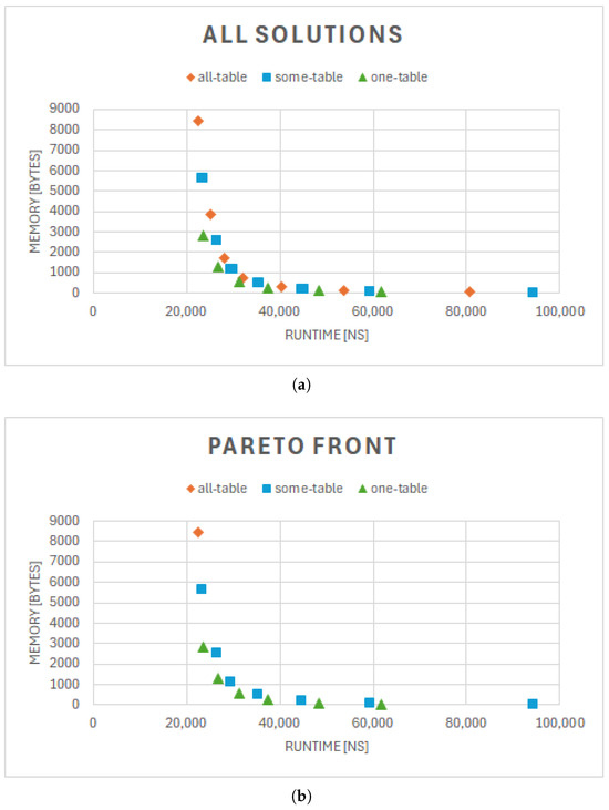
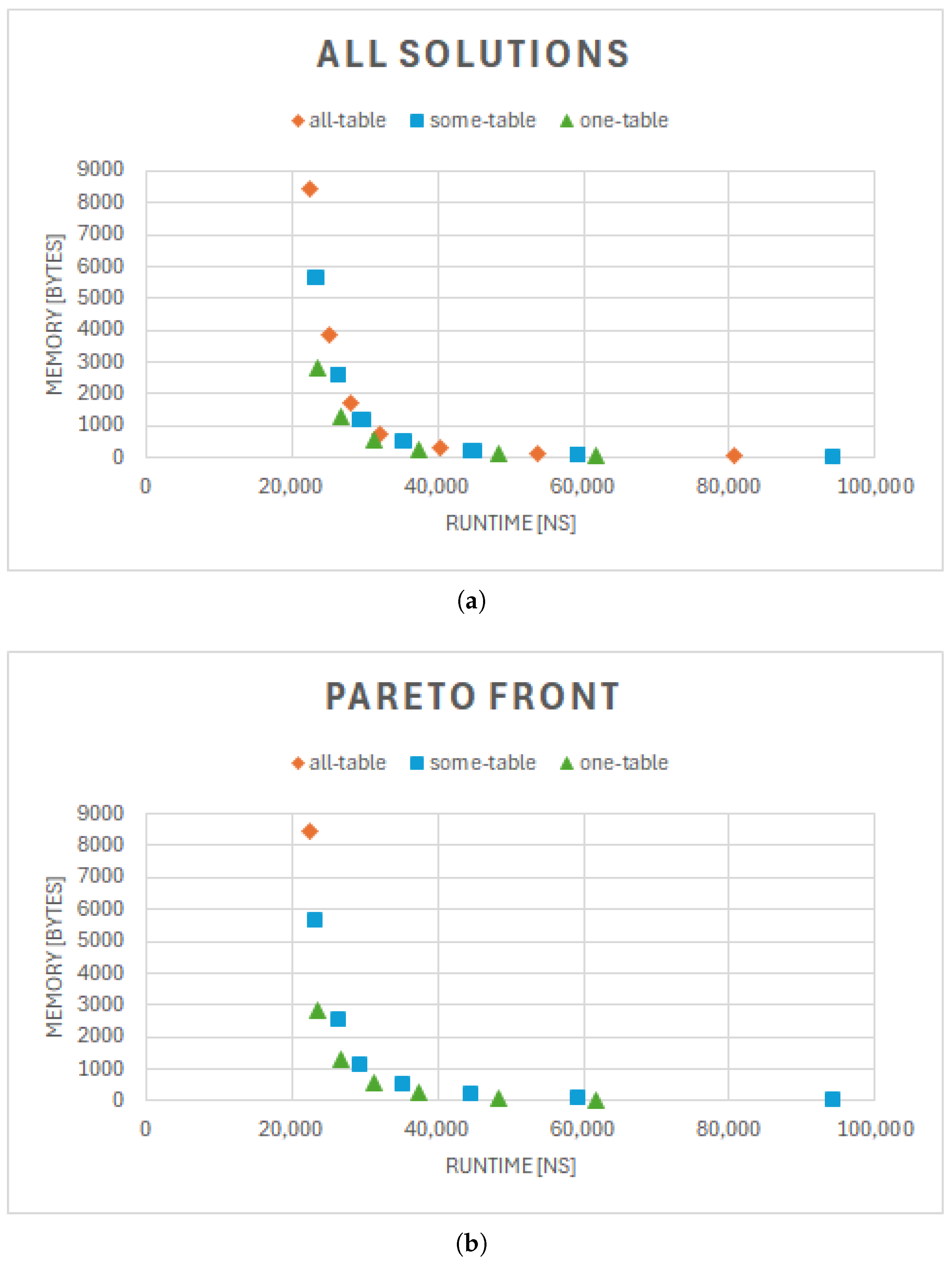
Figure 1 depicts runtime (averaged over all 10 strings to be decoded, and here the standard deviation is below 5% of the average) and table memory requirements of all tested solutions, together with the Pareto front resulting from these. From panel (a), we see that for each value of u, the all-table method with three tables is faster than the some-table method with two tables, which is faster than the one-table method with one table, which in turn is faster than the all-table method for $u-1$. This result confirms common wisdom that using larger tables and more tables improves speed. Additionally, the one-table method for $u=3$ (which is the minimum as there are codewords with this length) is already twice as fast as the method based on tree traversal, which we also implemented for comparison yet which we did not include in the figure.

Figure 1. (a) Runtime and table memory requirements for one-table, all-table and some-table methods with $u=2$ to 8 for Huffman code on 4 symbols with geometric distribution. (b) Pareto front of solutions in panel (a).

From panel (b), we see that the Pareto front only comprises one solution from the all-table method (point with highest memory consumption), which is for $u=8$, so that it is most likely only present because we did not consider $u=9$. For each u, we have a some-table solution and a one-table solution as part of the Pareto front, which indicates that the some-table method helps to provide more (and partly better) solutions on the Pareto front and thus helps the user to find a better compromise between speed and memory requirements.

If we consider each string to be decoded individually, the results are a little more diverse. For one string, both some-table methods are a bit slower than the one-table method for $u=3,5,7,8$. For another string, both some-table methods are a bit slower than the one-table method for $u=8$. For six further strings, one some-table method is a bit slower than the one-table method for one value of u, where the value of u differs for those strings ($u=3,5,7,8,8,8$).

When we compare the two some-table methods, the difference in speed is small, with each one being faster about half the time.

4.3. Symbols with Zipf Distribution

Here we use an alphabet with six symbols, where the probability of a symbol i is proportional to $1/i$ [10], i.e., the probabilities are $1/(i·H_i)$ where $H_i$ is the i-th harmonic number, resulting in probabilities $60/147$, $30/147$, $20/147$, $15/147$, $12/147$, $10/147$. The codewords of the corresponding Huffman code are 0, 100, 101, 110, 1110, 1111. Here, $S_{max}=\{\epsilon ,1,10,11,111\}$ so that the all-table method will use five tables, while the some-table method can use from two to four tables. Solving the Markov Chain for $u=2$ results in stationary properties of $4/9$ for $T_{\epsilon }$, $2/9$ for $T_1$ and $1/9$ for each further table. Thus, the some-table method will definitely use $T_{\epsilon }$ and $T_1$ and choose one or two of the other tables if the target number of tables is three or four, respectively.

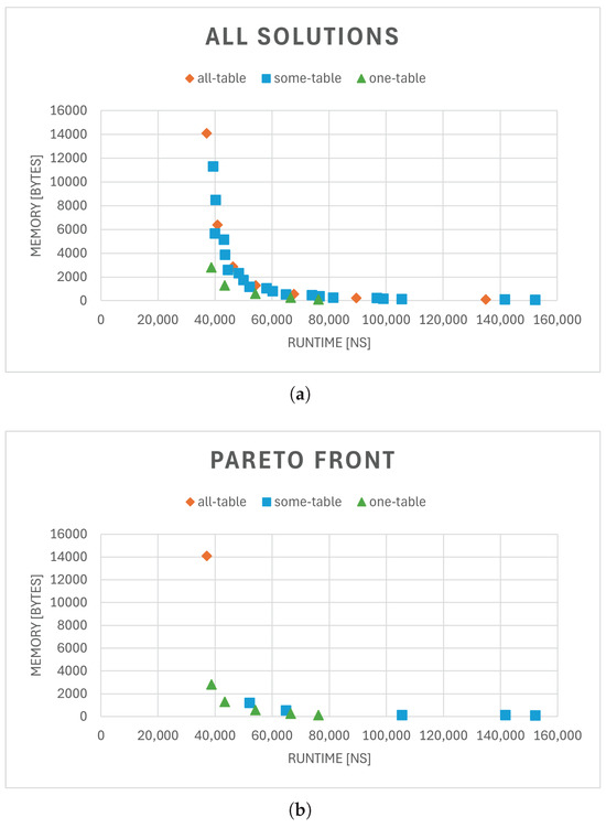
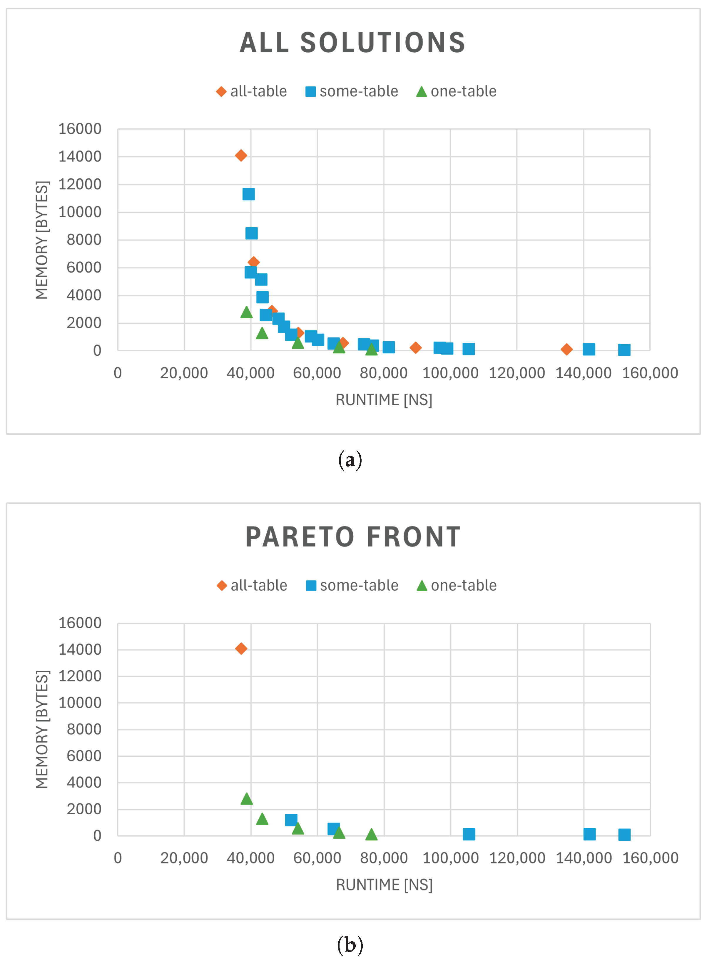
Figure 2 depicts runtime (averaged over all 10 strings to be decoded, where the standard deviation is below 5% of the average) and table memory requirements of all tested solutions, together with the Pareto front resulting from these. The Pareto front depicts a situation quite similar to the previous code: only one contribution from the all-table method, while the some-table method for different values of u mixes with the one-table method.

Figure 2. (a) Runtime and table memory requirements for the one-table, all-table and some-table methods with $u=2$ to 8 for Huffman code on 6 symbols with Zipf distribution. (b) Pareto front of solutions in panel (a).

Generally, the runtime relation is as it is before for a fixed value of u: the all-table method is the fastest, the some-table method gets slower with fewer tables, and the one-table method is the slowest. However, in some cases, the some-table method with only two tables is slower than the one-table table ($u=4$, $u=7$) and for $u=8$, only the some-table method with four tables matches the performance of the one-table method. Surprisingly, albeit not related to the some-table method, the performance of the one-table method for $u=6$ is similar to the performance of the all-table method for $u=5$, although the latter has more than twice the number of table elements than the former.

4.4. Discussion

The all-table method, although presented in previous works as the best acceleration method for the decoding of Huffman codes, does not really show in the Pareto fronts of the considered codes. In contrast, the one-table method, although seldom mentioned in textbooks or articles (cf. Section 5), has been stronger than expected and comprises a notable part of the Pareto fronts. The some-table method proved useful in filling the Pareto front and giving the user more choice to balance performance and memory requirements.

Our evaluation has been limited, as only two different codes, each with a small number of symbols, have been investigated. Also, as the number of tables to choose from in the heuristic is rather small, the appropriateness of the heuristics could not be tested fully.

5. Related Work

Decoding of prefix-free codes is not treated in all textbooks that we consulted. If mentioned, textbooks normally describe decoding by tree traversal. The one-table method is mentioned in only one textbook in thte German language [4], yet it is described as the usual acceleration of decoding. The all-table method is described in a textbook on compression [1] with a reference to [5].

The all-table variant is known from [5,6]. Both works mention the possibility of using a parameter u that is smaller than the maximum codeword length, so that $u=8$ for a byte-oriented software implementation is possible even if longer codewords exist. However, the possibility of our intermediate variants with some but not all tables is not mentioned in either paper. Choueka et al. [5] at least mention using reduced tables, i.e., tables of smaller size for cases where a prefix $\Delta$ at the end of one u-bit chunk is a prefix to only one codeword $w=\Delta |\mathrm{\Gamma }$ so that in table $D_{\Delta }^u$, only entries starting with $\mathrm{\Gamma }$ will be used, and consequently, that table can be reduced to size $2^{u-\left|\mathrm{\Gamma }\right|}$. Thus, their proposal can rather be seen as a post-optimization step applicable to the all-table and some-table methods.

Speed acceleration for Huffman decoding in recent years has focused on parallel decoding of different parts of longer codeword sequences on multicore processors, GPUs, and FPGAs [2,12,13], exploiting the self-synchronizing property of Huffman codes [14,15]. Iyer et al. [16] use multiple code trees, yet for different parts of a longer string to encode and decode in parallel. However, none of these works tries to improve on the decoding routine of a single decoding thread in software or decoding instance in hardware. So none strives to restrict shifts to fixed widths, e.g., bytes, in most instances, and none features tables that can be smaller than given from the maximum codeword length. Hwang et al. [8] at least mention the problem of memory consumption in Huffman decoding, yet for an embedded hardware accelerator.

Dynamic encoding and decoding, where the code tree is constructed with the data, is handled in [17], while we investigate static decoding, where decoding tables can be optimized.

While further improvements are possible for Huffman codes (e.g., by exploiting additional properties of canonical Huffman codes, cf. [18]), our algorithm works for any prefix-free code given by a binary code tree. If the code tree comprises inner nodes with only one child, non-decodable strings are possible, yet our decoding algorithm can also detect these. We summarize the related work in Table 2.

Table 2. Summary of related work.

Ref.	Year	Difference
[5]	1985	Reduced table size but no reduction in number of tables
[2]	2018	Parallel decoding on GPU, no improvement for single thread
[8]	2021	Reduction of memory consumption, yet for embedded hardware accelerator
[13]	2023	Parallel decoding on Multicore, no improvement for single thread
[12]	2024	Parallel decoding on FPGA, no improvement for single thread
[16]	2025	Multiple code trees/tables, yet for different input parts
[17]	2025	Investigates dynamic decoding

6. Conclusions and Future Work

We presented an algorithm to decode binary strings with sequences of codewords from a prefix-free code such as a Huffman code. The algorithmic design profited in decoding speed from using multiple tables and improved memory requirements by not using all tables, as in Chuoeka et al.’s and Sieminski’s all-table approaches [5,6]. Still, the new approach also kept the property of all-table approaches where the number of bits for the table index could be smaller than the length of the longest codeword, which reduced memory requirements for larger alphabet sizes where quite long codewords for seldom-used symbols exist.

Our evaluation with realistic codes (from geometric and Zipf distributions) demonstrated that in a two-dimensional Pareto front (where both decoding time and memory consumption should be minimized), configurations of our algorithm comprised about half of the non-dominated solutions in the Pareto front, while the all-table approach only appeared once. Hence, our algorithm could give developers more and better choices to balance decoding speed and memory requirements.

Future work will evaluate the performance of our algorithm for prefix-free codes other than Huffman codes, such as Shannon–Fano codes and other distributions of encoded symbols. Furthermore, we would like to investigate the applicability to codes that are not prefix-free but almost prefix-free and uniquely decodable.

References

- Salomon, D. Data Compression—The Complete Reference, 4th ed.; Springer: Berlin/Heidelberg, Germany, 2007. [Google Scholar]
- Weißenberger, A.; Schmidt, B. Massively Parallel Huffman Decoding on GPUs. In Proceedings of the 47th International Conference on Parallel Processing, ICPP 2018, Eugene, OR, USA, 13–16 August 2018; pp. 27:1–27:10. [Google Scholar] [CrossRef] [Scilit]
- Huffman, D.A. A Method for the Construction of Minimum-Redundancy Codes. Proc. IRE 1952, 40, 1098–1101. [Google Scholar] [CrossRef] [Scilit]
- Hoffmann, D.W. Einführung in die Informations–und Codierungstheorie, 2nd ed.; Springer: Berlin/Heidelberg, Germany, 2023. [Google Scholar]
- Choueka, Y.; Klein, S.T.; Perl, Y. Efficient Variants of Huffman Codes in High Level Languages. In Proceedings of the 8th Annual International ACM SIGIR Conference on Research and Development in Information Retrieval, Montréal, QC, Canada, 5–7 June 1985; pp. 122–130. [Google Scholar] [CrossRef] [Scilit]
- Sieminski, A. Fast Decoding of the Huffman Codes. Inf. Process. Lett. 1988, 26, 237–241. [Google Scholar] [CrossRef] [Scilit]
- Yoon, S.; Jun, S.; Cho, Y.; Lee, K.; Jang, H.; Han, T.H. Optimized Lossless Embedded Compression for Mobile Multimedia Applications. Electronics 2020, 9, 868. [Google Scholar] [CrossRef] [Scilit]
- Hwang, G.B.; Cho, K.N.; Han, C.Y.; Oh, H.W.; Yoon, Y.H.; Lee, S.E. Lossless Decompression Accelerator for Embedded Processor with GUI. Micromachines 2021, 12, 145. [Google Scholar] [CrossRef] [Scilit] [PubMed]
- Rajba, P.; Keller, J.; Mazurczyk, W. Entropy-Aware Secret Data Embedding for Network Storage Channels. In Proceedings of the International Conference on Availability, Reliability and Security (ARES 2025) International Workshops, Ghent, Belgium, 11–14 August 2025; pp. 327–345. [Google Scholar] [CrossRef] [Scilit]
- Zipf, G.K. The Psychobiology of Language; Houghton-Mifflin: New York, NY, USA, 1935. [Google Scholar]
- Piantadosi, S. Zipf’s word frequency law in natural language: A critical review and future directions. Psychon. Bull. Rev. 2014, 21, 1112–1130. [Google Scholar] [CrossRef] [Scilit] [PubMed]
- Liao, Y.; Wu, J.; Lu, W.; Li, X.; Yan, G. PHD: Parallel Huffman Decoder on FPGA for Extreme Performance and Energy Efficiency. In Proceedings of the 61st ACM/IEEE Design Automation Conference, DAC 2024, San Francisco, CA, USA, 23–27 June 2024; pp. 6:1–6:6. [Google Scholar] [CrossRef] [Scilit]
- Sarangi, S.; Baas, B.M. Energy-efficient canonical Huffman decoders on many-core processor arrays and FPGAs. Integration 2023, 88, 156–165. [Google Scholar] [CrossRef] [Scilit]
- Ferguson, T.J.; Rabinowitz, J.H. Self-synchronizing Huffman codes. IEEE Trans. Inf. Theory 1984, 30, 687–693. [Google Scholar] [CrossRef] [Scilit]
- Freiling, C.F.; Jungreis, D.S.; Théberge, F.; Zeger, K. Almost all complete binary prefix codes have a self-synchronizing string. IEEE Trans. Inf. Theory 2003, 49, 2219–2225. [Google Scholar] [CrossRef] [Scilit]
- Iyer, K.V.; Seshadri, K.; Srinivasulu, K. An Advancement in Huffman Coding with a Potential for Parallel Decoding. Concurr. Comput. Pract. Exp. 2025, 37, e70096. [Google Scholar] [CrossRef] [Scilit]
- Guguloth, E.; Vadtya, S.; Kudithi, T.; Shanmugam, M.R.; Banoth, A.N. FPGA implementation of high throughput encoder and decoder design of lossless canonical Huffman machine. Results Eng. 2025, 26, 105037. [Google Scholar] [CrossRef] [Scilit]
- Belu, S.; Coltuc, D. Fast Canonical Huffman Decoder. In Proceedings of the 14th International Conference on Communications, COMM 2022, Bucharest, Romania, 16–18 June 2022; pp. 1–6. [Google Scholar] [CrossRef] [Scilit]
Disclaimer/Publisher’s Note: The statements, opinions and data contained in all publications are solely those of the individual author(s) and contributor(s) and not of MDPI and/or the editor(s). MDPI and/or the editor(s) disclaim responsibility for any injury to people or property resulting from any ideas, methods, instructions or products referred to in the content. |
© 2025 by the authors. Licensee MDPI, Basel, Switzerland. This article is an open access article distributed under the terms and conditions of the Creative Commons Attribution (CC BY) license.