Kleene Algebra to Compute Invariant Sets of Dynamical Systems

Abstract

In this paper, we show that a basic fixed point method used to enclose the greatest fixed point in a Kleene algebra will allow us to compute inner and outer approximations of invariant-based sets for continuous-time nonlinear dynamical systems. Our contribution is to provide the definitions and theorems that will allow us to make the link between the theory of invariant sets and the Kleene algebra. This link has never be done before and will allow us to compute rigorously sets that can be defined as a combination of positive invariant sets. Some illustrating examples show the nice properties of the approach.

1. Introduction

In this paper, we deal with a dynamical system $\mathcal{S}$ defined by the following state equation:

$$\mathcal{S}:\dot{\mathbf{x}}\left(t\right)=\gamma \left(\mathbf{x}\left(t\right)\right)$$

(1)

where $\mathbf{x}\left(t\right)\in {\mathbb{R}}^n$ is the state vector and $\gamma :{\mathbb{R}}^n\mapsto {\mathbb{R}}^n$ is the evolution function of $\mathcal{S}$ [1,2]. Denote by ${\mathit{\phi }}_{\mathit{\gamma }}$ the flow map of (1); i.e., with the initial vector ${\mathbf{x}}_0=\mathbf{x}\left(0\right)$, the system $\mathcal{S}$ reaches the state ${\mathit{\phi }}_{\mathit{\gamma }}\left(t,{\mathbf{x}}_0\right)$ at time t. Our goal is to compute invariant sets [3] associated to the system with an algebraic approach, which is new in this context. Moreover, we propose to compute sets that can be expressed as a combination (union, intersection, image by a function, etc.) of invariant sets. In the application section of this paper, we will show why computing such combinations may be important in practice.

In particular, we will show the link between problems that can be expressed in terms of invariant sets and the Kleene algebra, the elements of which are automorphisms of a lattice [4]. We will take advantage of this algebraic structure to derive new efficient algorithms that are able to solve problems involving invariant sets that were not possible to compute with existing methods.

Our approach does not only provide a method to compute invariant sets. However, it allows us to compute sets that can be defined as a combination of invariant sets, which is the main contribution. We decided to explore an algebraic approach in order to get an elegant formalization of the problem resolution, as shown in several examples at the end of this paper.

A specific type of invariant set will be considered: the positive invariant set, which is an important concept in control [5], fault detection [6], safety [7], verification [8,9], or reachability [10].

A set $\mathbb{A}$ is positive invariant of (1) if we have

$$\mathbf{a}\in \mathbb{A},t\ge 0\Rightarrow {\mathit{\phi }}_{\mathit{\gamma }}\left(t,\mathbf{a}\right)\in \mathbb{A}.$$

(2)

The set of all positive invariant sets is a complete lattice; i.e., the union and the intersection of two positive invariant sets is positive invariant. A consequence is that given a set $\mathbb{A}$, the notion of the greatest positive invariant set contained in$\mathbb{X}$and smallest positive invariant set enclosing$\mathbb{A}$ can be defined. For instance, the greatest positive invariant set for (1) included in $\mathbb{A}$ is given by

$${\mathrm{Inv}}^{+}\left(\mathit{\gamma },\mathbb{A}\right)=\left\{\mathbf{a}|\forall t\ge 0,{\mathit{\phi }}_{\mathit{\gamma }}\left(t,\mathbf{a}\right)\in \mathbb{A}\right\}.$$

(3)

Methods exist to characterize positive invariant sets for specific cases such as for instance when $\mathit{\gamma }$ is linear [11,12,13] or discrete time [14]. Outer approximation can be computed by providing a model for approximation [15] or support functions [16]. Moreover, most approximations correspond to convex sets such as ellipsoids, zonotopes [17], or polytopes. These linear-based approaches can be extended to hybrid linear systems [18,19,20].

For continuous-time nonlinear systems, computing invariant sets is much more difficult, and different types of approaches can be extracted from the literature.

• The first approach is based on sampling. It has been used for instance by Saint Pierre [21] to rigorously compute viability kernel, which is a specific type of controlled invariant set. Bobiti and Lazar [22] also used a sampling-based method for stability verification of both continuous and discrete-time nonlinear systems. To get guaranteed results, an interval integration is often needed (see e.g., [23,24,25]).
• The second approach is based on Lyapunov theory [3,26] and is convenient for proving asymptotic stability of problems with an infinite time horizon. The principle is to find a parameter vector $\mathbf{p}$ or a Lyapunov-like function $V(\mathbf{p},\mathbf{x})$ such that the set

  $$\left\{\mathbf{x}\right|V(\mathbf{p},\mathbf{x})=0\mathrm{and}\dot{V}(\mathbf{p},\mathbf{x})\ge 0\}$$

  is empty. In such a case, the set $\mathbb{S}\left(\mathbf{p}\right)=\left\{\mathbf{x}\right|V(\mathbf{p},\mathbf{x})\le 0\}$ defines a positive invariant set. The function that is generally chosen for $V(\mathbf{p},\mathbf{x})$ is polynomial in the $x_i$’s and linear in the $p_j$’s. When $\mathit{\gamma }$ is polynomial, this choice for $V(\mathbf{p},\mathbf{x})$ makes it possible to use LMI/SOS/interval resolution techniques, which can be efficient when a low-dimensional approximation exists. This approach relies on assumptions such as the knowledge of an equilibrium point [27] or the polynomial property of the dynamics of the system [28], which is not always realistic.
• The third approach is based is based on occupation measures, which are adapted to a finite time horizon [27]. Now, it can also consider problems with infinite time horizon at the price of technical difficulties [29].
• The fourth approach is based a polygonal decomposition of the state space [30,31] and corresponds to the approach we will consider in the paper. For instance, in [30], a triangulated region yields an index filtration for a Morse decomposition of the flow on the system [32], which approximates the flow arbitrarily closely.

Different solvers such as SpaceEx [33,34] are available to compute numerically such invariant sets.

The paper proposes to compute inner and outer approximations of invariant sets in the general case where the system is continuous-time and nonlinear. More than that, it introduces for the first time an approach based on the Kleene algebra to compute sets that can be defined as operations on invariant sets. A possible application is the path planning and avoid problem [35], where we search for the set of all initial conditions for trajectories starting from of set $\mathbb{A}$ reaching the set $\mathbb{B}$ while avoiding the set $\mathbb{C}$. It is not possible to solve this type of problem rigorously using existing approaches.

This paper is organized as follows. Section 2 recalls some notions on lattices that will be needed to understand the Kleene algebra in Section 3. Then, the specific case where the elements of the Kleene algebra are made with automorphism is considered in Section 4. The link with invariant sets in dynamical systems is introduced in Section 5. Some illustrative test cases are given in Section 6. Section 7 concludes the paper.

2. Lattices

Invariant sets have a lattice structure [36], and this will allow us to formalize our problem in an algebraic form. This section recalls some classical definitions on lattices and provides some illustrations to understand the basic principles that are needed to understand our methodology.

2.1. Definitions

A lattice $\left(\mathcal{L},\le ,\wedge ,\vee \right)$ is a partially ordered set, closed under least upper and greatest lower bounds [37]. The least upper bound of x and y is called the join and is denoted by $x\vee y$. The greatest lower bound is called the meet and is written as $x\wedge y$.

A lattice $\mathcal{E}$ is complete if for all (finite or infinite) subsets $\mathcal{A}$ of $\mathcal{E}$, the least upper bound $\vee \mathcal{A}$ and the greatest lower bound $\wedge \mathcal{A}$ belong to $\mathcal{E}$. We define the top and the bottom of $\mathcal{E}$ as $\top =\vee \mathcal{E}$ and $\perp =\wedge \mathcal{E}$. A sublattice of a lattice $\left(\mathcal{L},\le \right)$ is a nonempty subset of $\mathcal{L}$ that is a lattice with the same meet and join operations ∨ and ∧ as $\mathcal{L}$.

2.2. Machine Lattice

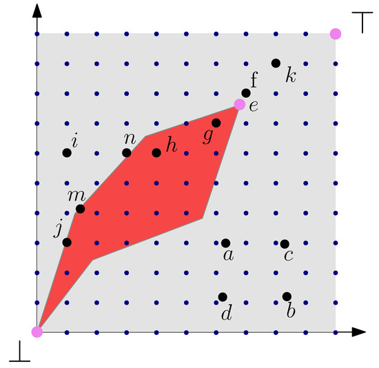
Consider a complete lattice $\left(\mathcal{L},\le ,\wedge ,\vee \right)$. A machine lattice $\left({\mathcal{L}}_M,\le ,\wedge ,\vee \right)$ of $\mathcal{L}$ is a complete sublattice of $\left(\mathcal{L},\le ,\wedge ,\vee \right)$ which is finite (thus, we can store it in the memory of a computer [38]). Moreover, both $\mathcal{L}$ and ${\mathcal{L}}_M$ have the same top ⊤ and bottom ⊥. This is illustrated by Figure 1, which can be interpreted as follows.

Figure 1. The grid corresponds to the machine lattice ${\mathcal{L}}_M$ associated to the lattice $\mathcal{L}$.

• The gray square represents $\mathcal{L}$.
• The element k is greater than f, since it is at its top right.
• The grid made with blue dots corresponds to ${\mathcal{L}}_M$.
• The variables $a,b,c,d$ all belong to $\mathcal{L}$, and we have $c=a\vee b$ and $d=a\wedge b$.
• The red polygon $\mathcal{P}$ is a sub-lattice of $\mathcal{L}$. Its bottom is ${\perp }_{\mathcal{P}}=\perp$ and its top is ${\top }_{\mathcal{P}}=e$.
• The element $i\in \mathcal{L}$ is inside $\left[{\perp }_{\mathcal{P}},{\top }_{\mathcal{P}}\right]$. Thus, there exists an element n in $\mathcal{P}$ which corresponds to the smallest element in $\mathcal{P}$, which is larger than i. There exists also an element m in $\mathcal{P}$ that corresponds to the greatest element in $\mathcal{P}$, which is smaller than i.
• The smallest machine interval containing e is $\left[g,f\right]$.

Remark 1.

In our context, the lattice $\mathcal{L}$ will correspond to the set of all subsets of ${\mathbb{R}}^n$ and ${\mathcal{L}}_M$ to the set of all machine sets (or mazes [39,40]). In Figure 1, the red polygon could represent the set of all positive invariant sets included in the set represented by e. The figure could also illustrate that given a set $\mathbb{A}$, there exists a smallest invariant set that contains $\mathbb{A}$, and there exists a largest element in $\mathcal{P}$, which is included in $\mathbb{A}$.

3. Kleene Algebra

The invariant sets of a dynamical system can be defined as fixed points of monotonic operators, which can be formalized elegantly using a Kleene algebra. The basic notions related to Kleene algebras are recalled in this section.

3.1. Definition

A Kleene algebra $\left(\mathcal{K},+,·,\ast \right)$ is a set $\mathcal{K}$ together with two binary operations $+:\mathcal{K}\times \mathcal{K}\to \mathcal{K}$ and $·:\mathcal{K}\times \mathcal{K}\to \mathcal{K}$ and one function $\ast :\mathcal{K}\to \mathcal{K}$, so that the axioms listed in the Table 1 are satisfied.

Table 1. Axioms/definitions of a star-continuous Kleene algebra.

Kleene algebra	$\left(\mathcal{K},+,·,\ast \right)$
Addition	$a+b$
Product	$a·b$
Associativity	$a+(b+c)=(a+b)+c$
	$a·(b·c)=(a·b)·c$
Commutativity	$a+b=b+a$
Distributivity	$a·(b+c)=(a·b)+(a·c)$
	$(b+c)·a=(b·a)+(c·a)$
Zero	$a+0=a$
One	$a·1=1·a=a$
Annihilation	$a·0=0·a=0$
Idempotence	$a+a=a$
Partial order	$a\le b\iff a+b=b$
Kleene star	$a^{\ast }=1+a+a·a+a·a·a+\dots$

The literature contains several inequivalent definitions of Kleene algebras and related algebraic structures [41]. Our definition differs when we introduce the Kleene operator: we assume star-continuity, which is needed as soon as infinite cardinal sets are considered.

Probably the mainstream definition is that of Kozen in [42], where the Kleene operator is defined formally by the following properties

$$\begin{array}{c}1+a{a}^{\ast }\le a^{\ast }\\ 1+a^{\ast }a\le a^{\ast }\\ ax\le x\Rightarrow a^{\ast }x\le x\\ xa\le x\Rightarrow x{a}^{\ast }\le x\end{array}$$

and the star-continuity is defined by

$$\begin{array}{c}x{a}^{\ast }y=\sum _{i\ge 0}x{a}^{i}y.\end{array}$$

Now, if we take $x=y=1,$ we get

$$a^{\ast }=1·a^{\ast }·1=\sum _{i\ge 0}1·a^i·1=\sum _{i\ge 0}{a}^i.$$

which corresponds to our definition.

The following proposition illustrates the fact that applying a Kleene star operator to a amounts to computing a fixed point. This will be used later in the algorithms.

Proposition 1.

Given a star continuous Kleene algebra $\left(\mathcal{K},+,·,\ast \right)$, we have

$${\left(1+a\right)}^{\infty }=\underset{i\to \infty }{lim}{\left(1+a\right)}^i=a^{\ast }$$

(4)

where

$$\begin{array}{ccc}{a}^0& =& 1\\ a^{i+1}& =& a·a^i\\ a^{\infty }& =& \underset{i\to \infty }{lim}{a}^i& (\mathit{if}\mathit{it}\mathit{exists})\end{array}$$

Proof. 

We first show by induction that

$${\left(1+a\right)}^n=\sum _{i\in \{0,n\}}{a}^i.$$

(5)

Assume that the proposition is true for $n.$ We have

$$\begin{array}{ccc}{\left(1+a\right)}^{n+1}& =& \left(1+a\right){\left(1+a\right)}^n\hfill \\ & \stackrel{\left(5\right)}{=}& \left(1+a\right)·\sum _{i\in \{0,n\}}{a}^i\hfill \\ & =& \left(\sum _{i\in \{0,n\}}{a}^i+a·\sum _{i\in \{0,n\}}{a}^i\right)\hfill \\ & =& \left(\sum _{i\in \{0,n\}}{a}^i+\sum _{i\in \{0,n\}}{a}^{i+1}\right)\hfill \\ & =& \left(\sum _{i\in \{0,n\}}{a}^i+\sum _{i\in \{1,n+1\}}{a}^i\right)\hfill \\ & =& \sum _{i\in \{0,n+1\}}{a}^i.\hfill \end{array}$$

Since the two sequences involved in (5) are equal, they have the same limit. Therefore,

$$\underset{n\to \infty }{lim}{\left(1+a\right)}^n=\underset{n\to \infty }{lim}\left(\sum _{i\in \{0,n\}}{a}^i\right)=\sum _{i\in \{0,\dots ,\infty \}}{a}^i=a^{\ast }.$$

□

3.2. Intervals

Consider a star-continuous Kleene algebra $\left(\mathcal{K},+,·,\ast \right)$. It is equipped with the order relation ≤ defined by $a\le b\iff a+b=b$ (see Table 1). We consider $\left({\mathcal{K}}_M,\le ,\wedge ,\vee \right)$ a machine lattice of $\mathcal{K}$ with respect to ≤, i.e.,

$$\begin{array}{ccccc}\left(i\right)& & a\wedge b& =& max\left\{c\in {\mathcal{K}}_M|c\le a,c\le b\right\}\\ & & & =& \sum \left\{c\in {\mathcal{K}}_M|c\le a,c\le b\right\}\\ \left(ii\right)& & a\vee b& =& min\left\{c\in {\mathcal{K}}_M|a\le c,b\le c\right\}\\ & & & =& a+b.\end{array}$$

The max and min are used since ${\mathcal{K}}_M$ is finite. To prove (i) we consider $c,d$ in ${\mathcal{K}}_M$. We have

$$\begin{array}{ccc}\left\{\begin{array}{c}c\le a\wedge b\\ d\le a\wedge b\end{array}\right.& \Rightarrow & \left\{\begin{array}{c}c\le a,c\le b\\ d\le a,d\le b\end{array}\right.\\ & \Rightarrow & \left\{\begin{array}{c}c+d\le a+a\\ c+d\le b+b\end{array}\right.\\ & \Rightarrow & \left\{\begin{array}{c}c+d\le a\\ c+d\le b\end{array}\right.\\ & \Rightarrow & \begin{array}{c}c+d\le a\wedge b\end{array}\end{array}$$

such that $c\le a,c\le b$ and $d\le a,d\le b$. To check that $a\vee b=a+b$ (in (ii)), it suffices to observe that $a\le a+b$ and that $b\le a+b$.

It can be shown that $\left({\mathcal{K}}_M,+,·,\ast \right)$ is also a Kleene algebra. Note that since ${\mathcal{K}}_M$ is finite, it is obviously star-continuous.

Definition 1.

An interval of $\left(\mathcal{K},+,·,\ast \right)$ is a subset $\left[a\right]$ of $\mathcal{K}$ that can be written as

$$\left[a\right]=\left[a^{-},a^{+}\right]=\left\{a\in \mathcal{K}|a^{-}\le a\le a^{+}\right\}$$

where $a^{-},a^{+}$ belong to ${\mathcal{K}}_M$.

Note that both ∅ and $\mathcal{K}$ are intervals of $\mathcal{K}$. Thus, an interval arithmetic similar to that proposed by Moore [43] for real numbers can be derived. This will be used later to compute with quantities defined as expressions of fixed point operators. As a consequence, if $a\in \left[a\right]=\left[a^{-},a^{+}\right]$, $b\in \left[b\right]=\left[b^{-},b^{+}\right]$, we have

$$\begin{array}{ccc}{\left[a^{-},a^{+}\right]}^{\ast }& =& \left[{\left(a^{-}\right)}^{\ast },{\left(a^{+}\right)}^{\ast }\right]\\ \left[a^{-},a^{+}\right]+\left[b^{-},b^{+}\right]& =& \left[a^{-}+b^{-},a^{+}+b^{+}\right]\\ \left[a^{-},a^{+}\right]·\left[b^{-},b^{+}\right]& =& \left[a^{-}·b^{-},a^{+}·b^{+}\right].\end{array}$$

(6)

due to the monotonicity of the operators $+,·,\ast$.

4. Kleene Algebra of Automorphisms

The notions presented in Section 2 and Section 3 can be seen as direct extensions of existing algebraic approaches related to lattices and Kleene algebra. In this section, we introduce automorphism-based Kleene algebras [4], which will allow us to make a first bridge between algebraic tools and invariant sets of nonlinear dynamical systems.

4.1. Automorphisms

Given a complete lattice $\left(\mathcal{L},\le ,\wedge ,\vee ,\perp ,\top \right)$, an automorphism of $\mathcal{L}$ is a function f:$\mathcal{L}\to \mathcal{L}$ such that

$$\begin{array}{ccccc}\left(\mathrm{i}\right)& & f\left(\top \right)& =& \top \\ \left(\mathrm{ii}\right)& & f\left(a\wedge b\right)& =& f\left(a\right)\wedge f\left(b\right)\end{array}.$$

(7)

As we will see later (see, e.g., Table 2), no property is assumed concerning the operator ∨.

Table 2. The set of automorphisms forms a star-continuous Kleene algebra.

Kleene Algebra	$\left(\mathcal{A}\left(\mathcal{L}\right),\wedge ,\circ ,\ast \right)$
Addition	$f\wedge g$
Product	$f\circ g$
Associativity	$f\wedge \left(g\wedge h\right)=\left(f\wedge g\right)\wedge h$
	$f\circ \left(g\circ h\right)=\left(f\circ g\right)\circ h$
Commutativity	$f\wedge g=g\wedge f$
Distributivity	$f\circ \left(g\wedge h\right)=\left(f\circ g\right)\wedge \left(f\circ h\right)$
	$\left(g\wedge h\right)\circ f=\left(g\circ f\right)\wedge \left(h\circ f\right)$
Zero	$f\wedge \top =f$
One	$f\circ \mathrm{Id}=\mathrm{Id}\circ f=f$
Annihilation	$f\circ \top =\top$
Idempotency	$f\wedge f=f$
Partial order	$f\ge g\iff f\wedge g=g$
Kleene star	$f^{\ast }=\mathrm{Id}\wedge f\wedge f^2\wedge f^3\wedge \dots$

We denote by $\mathcal{A}\left(\mathcal{L}\right)$ the set of automorphisms of $\mathcal{L}$.

Proposition 2.

If $f,g$ are in $\mathcal{A}\left(\mathcal{L}\right)$, then:

$$\begin{array}{c}\begin{array}{ccc}\left(\mathrm{i}\right)& & a\le b\Rightarrow f\left(a\right)\le f\left(b\right)\hfill \\ \left(\mathrm{ii}\right)& & f\wedge g\in \mathcal{A}\left(\mathcal{L}\right)\hfill \\ \left(\mathrm{iii}\right)& & f\circ g\in \mathcal{A}\left(\mathcal{L}\right)\hfill \\ \left(\mathrm{iv}\right)& & \mathrm{Id}\wedge f\wedge f^2\wedge f^3\wedge \dots \in \mathcal{A}\left(\mathcal{L}\right)\hfill \end{array}\end{array}$$

(8)

where the function $f\wedge g$ is defined by $\left(f\wedge g\right)\left(a\right)=f\left(a\right)\wedge f\left(a\right).$

Proof. 

(i) We have

$$\begin{array}{ccc}a\le b& \iff & a=b\wedge a\hfill \\ & \Rightarrow & f\left(a\right)=f\left(b\wedge a\right)\hfill & & \hfill \\ & \iff & f\left(a\right)=f\left(b\right)\wedge f\left(a\right)\hfill & & (\mathrm{see} \text{Eq} 7,\mathrm{ii})\hfill \\ & \Rightarrow & f\left(a\right)\le f\left(b\right).\hfill \end{array}$$

(9)

(ii) We have $\left(f\wedge g\right)\left(\top \right)=\top \wedge \top =\top$. Moreover,

$$\begin{array}{ccc}\left(f\wedge g\right)\left(a\wedge b\right)& =& \left(f\left(a\wedge b\right)\right)\wedge \left(g\left(a\wedge b\right)\right)\hfill \\ & =& f\left(a\right)\wedge f\left(b\right)\wedge g\left(a\right)\wedge g\left(b\right)\hfill \\ & =& \left(f\wedge g\right)\left(a\right)\wedge \left(f\wedge g\right)\left(b\right)\hfill \end{array}$$

(10)

(iii) We have $f\circ g\left(\top \right)=f\left(\top \right)=\top$. Moreover,

$$\begin{array}{ccc}\left(f\circ g\right)\left(a\wedge b\right)& =& f\left(g\left(a\right)\wedge g\left(b\right)\right)\\ & =& \left(f\circ g\right)\left(a\right)\wedge \left(f\circ g\right)\left(b\right)\end{array}$$

(11)

(iv) It corresponds to the Kleene operator and is a direct consequence of (ii), (iii). □

Proposition 3.

Assume that for $f\in \mathcal{A}\left(\mathcal{L}\right)$, $f^{\ast }=\mathrm{Id}\wedge f\wedge f^2\wedge f^3\wedge \dots$ exists (star-continuity assumption), then the set $\left(\mathcal{A}\left(\mathcal{L}\right),\wedge ,\circ ,\ast \right)$ is a Kleene algebra.

Proof. 

We need to check all properties of Table 2. In the two tables, the symbols of the operators changed: + corresponds to ∧, * corresponds to ∘, and ≥ corresponds to ≤. To prove the distributivity $f\circ \left(g\wedge h\right)=\left(f\circ g\right)\wedge \left(f\circ h\right)$, we proceed as follows:

$$\begin{array}{ccc}f\circ \left(g\wedge h\right)\left(a\right)& =& f\circ \left(g\left(a\right)\wedge h\left(a\right)\right)\\ & \stackrel{(7,ii)}{=}& \left(f\circ g\right)\left(a\right)\wedge \left(f\circ h\right)\left(a\right).\end{array}$$

(12)

All other properties can be proved similarly. □

Remark 2.

The relation order for automorphism has been chosen backward (i.e., ≥ instead of ≤). This choice is motivated by the fact that the inclusion order will be used later, and we will have the following correspondences: $\le \leftrightarrow \subset ,\wedge \leftrightarrow \cap$.

Proposition 4.

The fixed points of $\mathrm{Id}\wedge f$ correspond to that of $f^{\ast }$,i.e.,

$$\mathrm{Fix}\left(f^{\ast }\right)=\left\{a|f^{\ast }\left(a\right)=a\right\}=\mathrm{Fix}\left(\mathrm{Id}\wedge f\right)$$

(13)

Proof. 

The proof is decomposed in two parts. In the first part, we prove that $\mathrm{Fix}\left(\mathrm{Id}\wedge f\right)\subset \mathrm{Fix}\left(f^{\ast }\right)$ and in the second part, we prove the inverse.

(1)

We have

$$\begin{array}{ccc}(\mathrm{Id}\wedge f)\left(x\right)=x& \Rightarrow & \forall i\ge 1,{(\mathrm{Id}\wedge f)}^i\left(x\right)=x\\ & \Rightarrow & {(\mathrm{Id}\wedge f)}^{\infty }\left(x\right)=x\\ & \iff & f^{\ast }\left(x\right)=x\end{array}$$

since, from (4), we have ${\left(\mathrm{Id}\wedge f\right)}^{\infty }=f^{\ast }$. Thus, $\mathrm{Fix}\left(\mathrm{Id}\wedge f\right)\subset \mathrm{Fix}\left(f^{\ast }\right).$

(2)

We now want to prove the inverse inclusion: $\mathrm{Fix}\left(f^{\ast }\right)\subset \mathrm{Fix}\left(\mathrm{Id}\wedge f\right)$.

We first prove by induction that

$$\forall i\ge 0,{(\mathrm{Id}\wedge f)}^i\ge {(\mathrm{Id}\wedge f)}^{i+1}.$$

(14)

From the partial order property of Table 2, we have

$$\mathrm{Id}\ge (\mathrm{Id}\wedge f)\iff \mathrm{Id}\wedge (\mathrm{Id}\wedge f)=\mathrm{Id}\wedge f$$

(15)

since $\mathrm{Id}\wedge (\mathrm{Id}\wedge f)=(\mathrm{Id}\wedge \mathrm{Id})\wedge f=\mathrm{Id}\wedge f$, we get that the right-hand side of (15) is true and thus $\mathrm{Id}\ge \mathrm{Id}\wedge f$ is true. This means that for $i=0,$ (14) is true.

Assume now that (14) is true for i, let us check that it is true for $i+1.$ From Proposition 2 (i), we get that

$$f\ge g\Rightarrow h\circ f\ge h\circ g.$$

With the substitution $f\to {(\mathrm{Id}\wedge f)}^i,g\to {(\mathrm{Id}\wedge f)}^{i+1},h\to \mathrm{Id}\wedge f$, we get

$${(\mathrm{Id}\wedge f)}^i\ge {(\mathrm{Id}\wedge f)}^{i+1}\Rightarrow (\mathrm{Id}\wedge f)\circ {(\mathrm{Id}\wedge f)}^i\ge (\mathrm{Id}\wedge f)\circ {(\mathrm{Id}\wedge f)}^{i+1}.$$

Since (14) is true for i, we get

$${(\mathrm{Id}\wedge f)}^{i+1}\ge {(\mathrm{Id}\wedge f)}^{i+2},$$

thus, we have proved (14).

From (14), we get ${(\mathrm{Id}\wedge f)}^i$ is a decreasing sequence and thus

$$\mathrm{Id}\ge (\mathrm{Id}\wedge f)\ge {(\mathrm{Id}\wedge f)}^i\ge {(\mathrm{Id}\wedge f)}^{\infty }.$$

Take a fixed point x of ${(\mathrm{Id}\wedge f)}^{\infty }$, we get

$$x\ge (\mathrm{Id}\wedge f)\left(x\right)\ge {(\mathrm{Id}\wedge f)}^{\infty }\left(x\right)=x,$$

thus, $(\mathrm{Id}\wedge f)\left(x\right)=x$, which implies that x is also a fixed point of $\mathrm{Id}\wedge f$. □

Since f is a monotonic, so is $\mathrm{Id}\wedge f$ and $f^{\ast }$. From the Knaster–Tarski theorem, we deduce that $\mathrm{Fix}\left(f^{\ast }\right)$ is a complete sublattice of $\mathcal{L}$.

4.2. Factorization

In this paper, we want to compute expressions involving the Kleene star operator. For efficiency reasons, we want to avoid reaching the fixed point each time the star operator is used. Ideally, we would like to have a unique fixed point to be reached. For this, we need to transform an expression containing several stars into an expression with only one star. Equivalently, we want to factorize the fixed point operator as much as possible. For this, we can use the factorization rules such as [42]:

$$\begin{array}{c}{f}^{\ast }\wedge f^{\ast }=f^{\ast }\\ f^{\ast }\circ f^{\ast }=f^{\ast }\\ {\left(f^{\ast }\right)}^{\ast }=f^{\ast }\\ {\left(f^{\ast }\wedge g^{\ast }\right)}^{\ast }={\left(f\wedge g\right)}^{\ast }\end{array}$$

(16)

but we can do more. Assume for instance that we have to compute

$$f^{\ast }\left(a\right)\wedge g^{\ast }\left(b\right),$$

(17)

we understand that it is not necessary to compute $f^{\ast }\left(a\right)$ and $g^{\ast }\left(b\right)$ independently to finally observe that we get ⊥. For instance, we may have spent a lot of time to compute accurately $f^{\ast }\left(a\right)$ and a few milliseconds to get that $g^{\ast }\left(b\right)=\perp$ to finally reach the conclusion that $f^{\ast }\left(a\right)\wedge g^{\ast }\left(b\right)=\perp$. As a result, we need to develop some specific algorithms taking into account that calling closures has a cost. The factorization allows us to reduce several fixed point iterations into a single one. This can be used to increase the speed of convergence of fixed point algorithms.

4.3. Intervals

Given a lattice $\left(\mathcal{L},\le ,\wedge ,\vee \right)$ and an automorphism $f\in \mathcal{A}\left(\mathcal{L}\right)$, we want to compute $f^{\ast }\left(a\right)$ where $a\in \mathcal{L}$. We consider also a machine lattice ${\mathcal{L}}_M$ of $\mathcal{L}$. An automorphism of ${\mathcal{L}}_M$ is called a machine automorphism. As seen in SubSection 3.2, since $\mathcal{A}\left(\mathcal{L}\right)$ is a Kleene algebra, we can define intervals in $\mathcal{A}\left(\mathcal{L}\right)$.

Definition 2.

An interval of $\mathcal{A}\left(\mathcal{L}\right)$ is a subset $\left[f\right]$ of $\mathcal{A}\left(\mathcal{L}\right)$, which can be written as

$$\left[f\right]=\left[f^{-},f^{+}\right]=\left\{f\in \mathcal{A}\left(\mathcal{L}\right)|f^{-}\le f\le f^{+}\right\}$$

(18)

where $f^{-},f^{+}$ belong to $\mathcal{A}\left({\mathcal{L}}_M\right)$.

Proposition 5.

We have

$$\begin{array}{c}\mathit{Fix}\left({\left(f^{-}\right)}^{\ast }\right)\subset {\mathcal{L}}_M\cap \mathit{Fix}\left(f^{\ast }\right)\subset \mathit{Fix}\left({\left(f^{+}\right)}^{\ast }\right).\hfill \end{array}$$

(19)

Proof. 

Let us first prove the first inclusion. First, since ${\left(f^{-}\right)}^{\ast }\in \mathcal{A}\left({\mathcal{L}}_M\right)$, all its fixed points are inside ${\mathcal{L}}_M$. We have

$$\begin{array}{ccc}a\in \mathrm{Fix}\left({\left(f^{-}\right)}^{\ast }\right)& \Rightarrow & {\left(f^{-}\right)}^{\ast }\left(a\right)=a,\\ & \iff & a\wedge f^{-}\left(a\right)=a& & (\mathrm{see} (13\left)\right)\hfill \\ & \Rightarrow & a\wedge f\left(a\right)\ge a& & (\sin \mathrm{ce}{f}^{-}\le f)\hfill \\ & \iff & a\wedge f\left(a\right)=a& & (\sin \mathrm{ce}a\wedge x\le a)\hfill \\ & \iff & f^{\ast }\left(a\right)=a& & (\mathrm{see} (13\left)\right).\hfill \end{array}$$

Let us now prove the second inclusion. We have

$$\begin{array}{cc}& a\in {\mathcal{L}}_M\cap \mathrm{Fix}\left(f^{\ast }\right)\\ \Rightarrow & f^{\ast }\left(a\right)=a,a\in {\mathcal{L}}_M\\ \iff & a\wedge f\left(a\right)=a,a\in {\mathcal{L}}_M& (\mathrm{see} (13\left)\right)\\ \Rightarrow & a\wedge f^{+}\left(a\right)\ge a& (\sin \mathrm{ce}f\le f^{+})\\ \iff & a\wedge f^{+}\left(a\right)=a& (\sin \mathrm{ce}a\wedge x\le a)\\ \iff & {\left(f^{+}\right)}^{\ast }\left(a\right)=a& (\mathrm{see} (13\left)\right)\end{array}$$

□

Theorem 1.

If $a\in \left[a^{-},a^{+}\right]$, where $a^{-},a^{+}$ both belong to ${\mathcal{L}}_M$, then

$$\begin{array}{ccc}\left(\mathrm{i}\right)& & f^{\ast }\left(a\right)\in \left[{\left(f^{-}\right)}^{\ast }\left(a^{-}\right),{\left(f^{+}\right)}^{\ast }\left(a^{+}\right)\right]\hfill \\ \left(\mathrm{ii}\right)& & f^{\ast }\circ {\left(f^{-}\right)}^{\ast }\left(a^{-}\right)={\left(f^{-}\right)}^{\ast }\left(a^{-}\right)\hfill \\ \left(\mathrm{iii}\right)& & f^{\ast }\left(a\right)\le {\left(\mathit{Id}\wedge f^{+}\right)}^i\left(a^{+}\right),\forall i\ge 0\hfill \end{array}$$

(20)

Remark 3.

The membership relation (i) means that we are able to compute in a finite time an enclosure of the fixed point $f^{\ast }\left(a\right)$. Relation (ii) states that the fixed point obtained by ${\left(f^{-}\right)}^{\ast }$ is a fixed point of $f^{\ast }$. However, this is not true for ${\left(f^{+}\right)}^{\ast }$. Relation (iii) tells us that at each iteration i, we have an upper bound for the solution $f^{\ast }\left(a\right)$, but we need to reach the fixed point to get a lower approximation ${\left(f^{-}\right)}^{\ast }\left(a^{-}\right)$ of $f^{\ast }\left(a\right)$.

Proof. 

(i) is a consequence of the fact that $f^i\left(a\right)\in \left[{\left(f^{-}\right)}^i\left(a^{-}\right),{\left(f^{+}\right)}^i\left(a^{+}\right)\right]$.

(ii) Since ${\left(f^{-}\right)}^{\ast }\circ {\left(f^{-}\right)}^{\ast }\left(a^{-}\right)={\left(f^{-}\right)}^{\ast }\left(a^{-}\right)$, the quantity ${\left(f^{-}\right)}^{\ast }\left(a^{-}\right)$ is a fixed point of ${\left(f^{-}\right)}^{\ast }$. Now, from (19), we have $\mathrm{Fix}\left({\left(f^{-}\right)}^{\ast }\right)\subset \mathrm{Fix}\left(f^{\ast }\right).$ Therefore, ${\left(f^{-}\right)}^{\ast }\left(a^{-}\right)$ is also a fixed point of $f^{\ast }$, i.e., $f^{\ast }\circ {\left(f^{-}\right)}^{\ast }\left(a^{-}\right)={\left(f^{-}\right)}^{\ast }\left(a^{-}\right)$.

(iii) We have

$$\begin{array}{ccccc}{f}^{\ast }\left(a\right)& =& {\left(\mathrm{Id}\wedge f\right)}^{\infty }\left(a\right)& \le & {\left(\mathrm{Id}\wedge f\right)}^i\left(a\right)\\ & \le & {\left(\mathrm{Id}\wedge f^{+}\right)}^i\left(a\right)& \le & {\left(\mathrm{Id}\wedge f^{+}\right)}^i\left(a^{+}\right)\end{array}$$

□

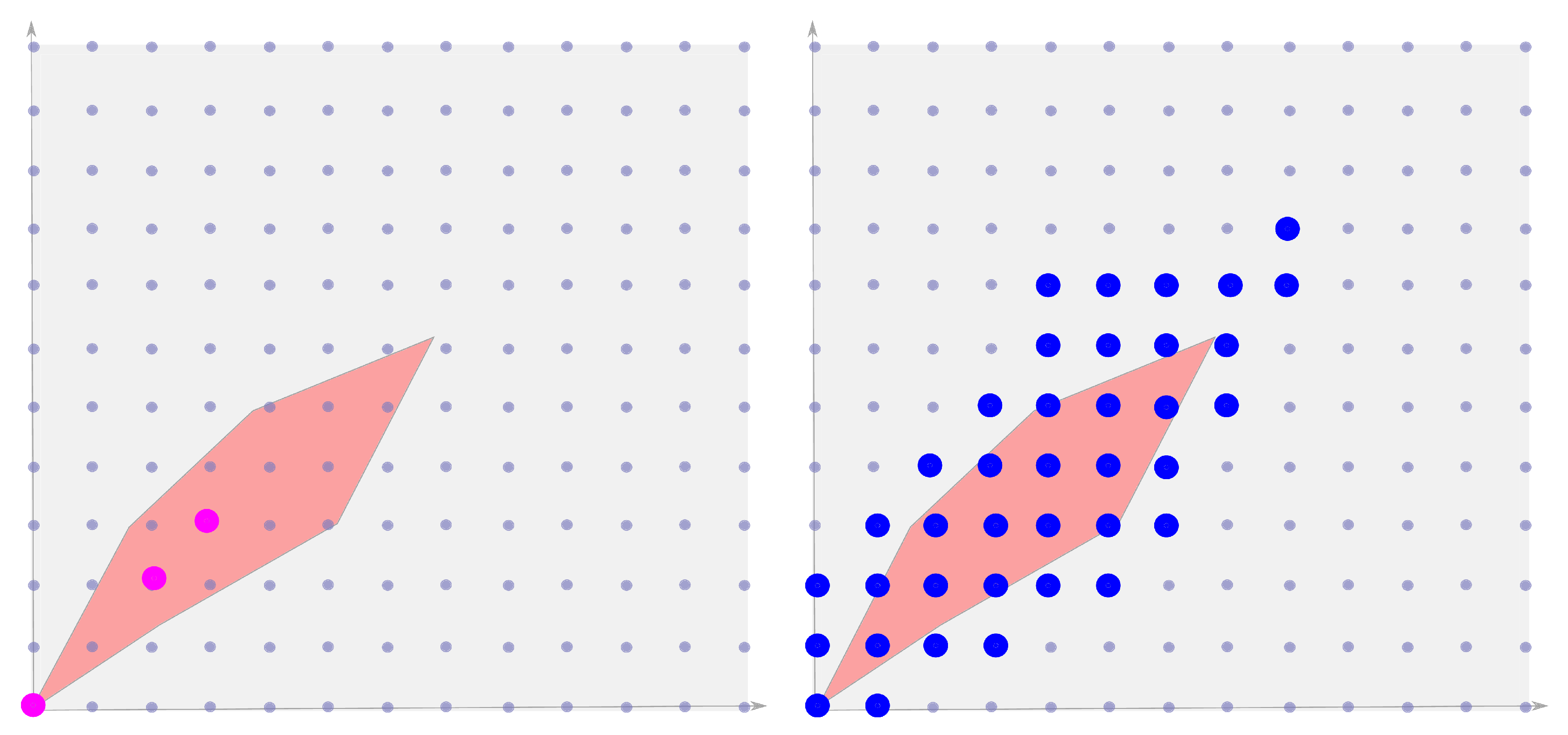
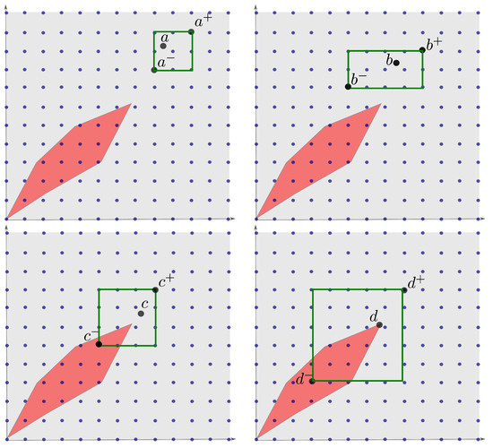
The inclusion (iii) is illustrated by Figure 2 where the grid corresponds to ${\mathcal{L}}_M$, the magenta points correspond to $\mathrm{Fix}\left({\left(f^{-}\right)}^{\ast }\right)$, the blue points correspond to $\mathrm{Fix}\left({\left(f^{+}\right)}^{\ast }\right)$, and the light red polygon corresponds to $\mathrm{Fix}\left(f^{\ast }\right)$.

Figure 2. Fixed points $\mathrm{Fix}\left({\left(f^{-}\right)}^{\ast }\right)$ in magenta, $\mathrm{Fix}\left({\left(f^{+}\right)}^{\ast }\right)$ in blue, and $\mathrm{Fix}\left(f^{\ast }\right)$ is the light red polygon.

4.4. Algorithm to Find the Greatest Fixed Point

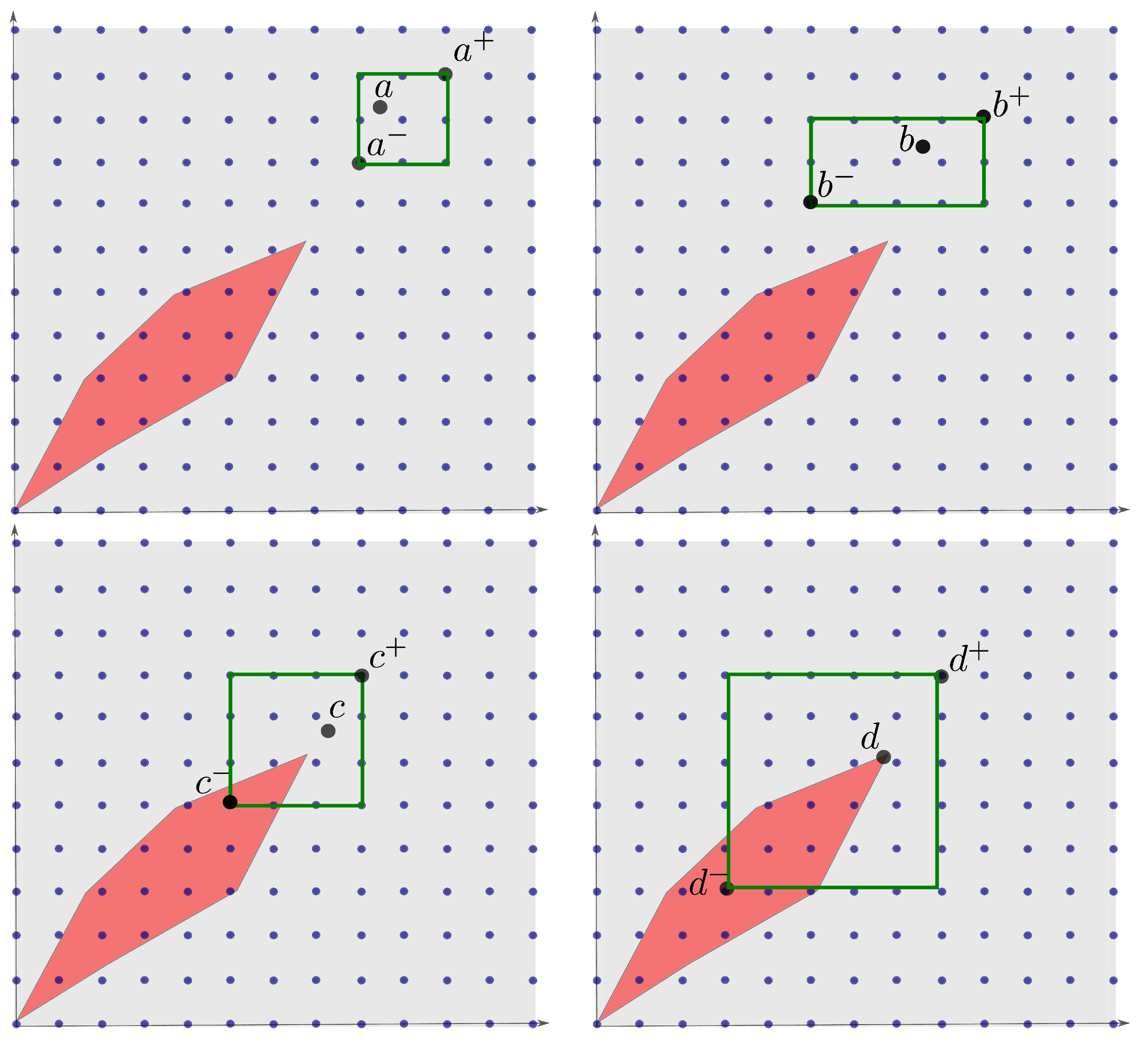
We propose here an interval algorithm [44] to compute $f^{\ast }\left(a\right)$, where $a\in \left[a\right]=\left[a^{-},a^{+}\right]$. We assume that we have an interval $\left[f\right]=\left[f^{-},f^{+}\right]$ containing f, where $f^{-},f^{+}$ belong to $\mathcal{A}\left({\mathcal{L}}_M\right)$. From Equation (20), we know that

$$f^{\ast }\left(a\right)\in \left[{\left(f^{-}\right)}^{\ast }\left(a^{-}\right),{\left(\mathrm{Id}\wedge f^{+}\right)}^i\left(a^{+}\right)\right].$$

(21)

To compute $f^{\ast }\left(a\right)$, we apply the sequence of interval operations defined by

$$\begin{array}{ccc}\left[x\right]\left(i+1\right)& =& \left(\mathrm{Id}\wedge \left[f\right]\right)\left(\left[x\right]\left(i\right)\right)\\ \left[x\right]\left(0\right)& =& \left[a\right]\end{array}$$

(22)

up to the fixed point. From Theorem 1, we get a guaranteed approximation of $f^{\ast }\left(a\right)$. Since ${\mathcal{L}}_M$ is finite, the algorithm always terminates. The principle of the algorithm is illustrated by Figure 3. First, a is approximated by an interval $\left[a^{-},a^{+}\right]$ of $\mathcal{A}\left({\mathcal{L}}_M\right)$. Then, we compute $\left(\mathrm{Id}\wedge \left[f\right]\right)\left(\left[a\right]\right)$, which corresponds to $\left[b\right]=\left[b^{-},b^{+}\right]$. Then, we compute $\left(\mathrm{Id}\wedge \left[f\right]\right)\left(\left[b\right]\right)$, which corresponds to $\left[c\right]=\left[c^{-},c^{+}\right]$. The last subfigure corresponds to the fixed point interval $\left[d\right]=\left(\left[f^{\ast }\right]\right)\left(\left[a\right]\right)$ which contains the solution $f^{\ast }\left(a\right)$.

Figure 3. Algorithm that computes an approximation of $f^{\ast }\left(a\right),a\in \left[a\right]$.

The sequence (4) provides a guaranteed enclosure for the solution, and the accuracy is related to the precision we used to define the machine lattice ${\mathcal{L}}_M$. Once the algorithm terminates, if we are not satisfied by the quality of the approximation, we should restart from the beginning by redefining ${\mathcal{L}}_M$ with a finer level of granularity.

Remark 4.

In our implementation, a multi-scale approach is used for more efficiency and more accuracy: once the fixed point interval $\left[d^{-},d^{+}\right]$ is reached, we build a new grid inside the interval $\left[d^{-},d^{+}\right]$. We also combine with an inflation process, which increases $d^{-}$ without overtaking the solution d. More precisely, in Figure 3, we may increase $d^{-}$ top-right still staying inside the red polygon in order to get a more accurate approximation for the solution d. We called this process inflation, since in the context of this paper, the points of the figure correspond to subsets of ${\mathbb{R}}^n$ equipped with the order relation is ⊂. When we increase d, we may understand that we inflate the set corresponding to $d^{-}$ still being included in the solution set corresponding to d.

5. Application to Dynamical Systems

In this section, we show that the previous algorithm can directly be used to compute invariant sets of continuous-time dynamical systems. Furthermore, we will show that we are able to compute sets that can be defined as a combination of invariant sets.

5.1. Greatest Positive Invariant

Consider the system $\mathcal{S}$ defined by Equation (1). The power set $\mathcal{P}\left({\mathbb{R}}^n\right)$ of the state space ${\mathbb{R}}^n$ and equipped with $\cap ,\cup$ is a lattice. We denote by $\left(\mathcal{A}\left(\mathcal{P}\left({\mathbb{R}}^n\right)\right),\cap ,\circ ,\ast \right)$ the associated set of automorphisms. We want to find an automorphism $\overrightarrow{f}$ in $\mathcal{A}\left(\mathcal{P}\left({\mathbb{R}}^n\right)\right)$ that can be enclosed between two machine automorphisms and such that ${\overrightarrow{f}}^{\ast }\left(\mathbb{A}\right)$ corresponds to the greatest positive invariant set included in $\mathbb{A}$, i.e.,

$$\begin{array}{ccc}{\overrightarrow{f}}^{\ast }\left(\mathbb{A}\right)& =& \left\{\mathbf{a}\in \mathbb{A}|\forall t\ge 0,{\mathit{\phi }}_{\mathit{\gamma }}(t,\mathbf{a})\in \mathbb{A}\right\}\end{array}$$

(23)

We may find some tools for that such as CAPD [24] or a tube approach [45] devoted to this type of problem. Now, these types of approaches only consider a finite time integration and are unable to compute the fixed point (23) in a reasonable time as shown in [46,47]. Therefore, it is important to build an automorphism $\overrightarrow{f}$, which is fast to evaluate and that will converge quickly. This can be done by using an Eulerian positive predictor [10], which analyzes the geometry of the vector field associated to the dynamic $\dot{\mathbf{x}}\left(t\right)=\mathit{\gamma }\left(\mathbf{x}\left(t\right)\right)$ of the system without performing any time integration. We propose to use a discretization of the state space using mazes [31]. Mazes correspond to a polygonal decomposition of the state space coupled with an interval enclosure for $\mathit{\gamma }\left(\mathbf{x}\right)$, which is valid inside the corresponding polygon. This decomposition by mazes can be interpreted as an interval of dynamics with a lower bound and an upper bound. The polygonal representation associated to the maze is a discrete object that can be represented in the memory of the computer by floating point numbers. It will be used to approximate from inside and from outside the sequence of sets that should converge in a finite number of iterations to the invariant set we want to compute. Equivalently, the polygonal representation corresponds to the machine lattice we use in our implementation to represent subsets of ${\mathbb{R}}^n$.

5.2. Paths

Definition 3.

Given a point$\mathbf{a}$and the system$\mathcal{S}:\dot{\mathbf{x}}\left(t\right)=\mathit{\gamma }\left(\mathbf{x}\left(t\right)\right)$. The path associated to $\mathbf{a}$ is defined as

$${\Psi }_{\mathit{\gamma }}\left(\mathbf{a}\right)=\left\{\mathbf{z}|\forall \epsilon >0,\exists t_1>0,\parallel {\mathit{\phi }}_{\mathit{\gamma }}(t_1,\mathbf{a})-\mathbf{z}\parallel \le \epsilon \right\}.$$

(24)

Equivalently, we can write

$${\Psi }_{\mathit{\gamma }}\left(\mathbf{a}\right)={\mathit{\phi }}_{\mathit{\gamma }}\left(\left[0,\infty \right],\mathbf{a}\right).$$

(25)

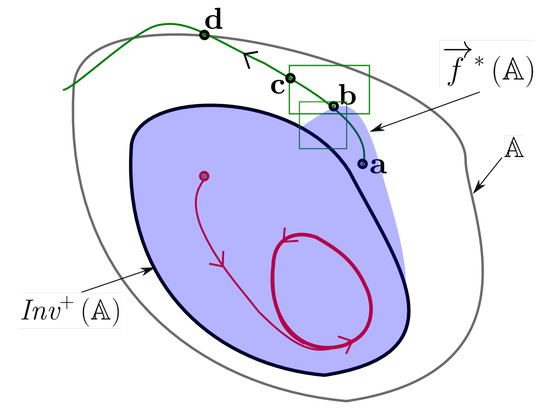
The path ${\Psi }_{\mathit{\gamma }}\left(\mathbf{a}\right)$ is a closed set and contains the equilibrium points or cycles to which the system will converge from $\mathbf{a}$.

Definition 4. 

(Path inside a region). Consider the system (1), a region $\mathbb{Y}$, and a point $\mathbf{a}\in \mathbb{Y}.$ We define the path inside $\mathbb{Y}$ as ${\Psi }_{\mathit{\gamma }|\mathbb{Y}}\left(\mathbf{a}\right)$ where the function $\mathit{\gamma }|\mathbb{Y}$ is defined as

$$\left(\mathit{\gamma }|\mathbb{Y}\right)\left(\mathbf{x}\right)=\left\{\begin{array}{ccc}\mathit{\gamma }\left(\mathbf{x}\right)& & \mathrm{if}\mathbf{x}\in \mathbb{Y}\\ \mathbf{0}& & \mathit{otherwize}\end{array}\right.$$

(26)

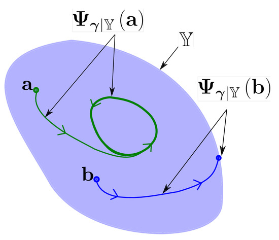
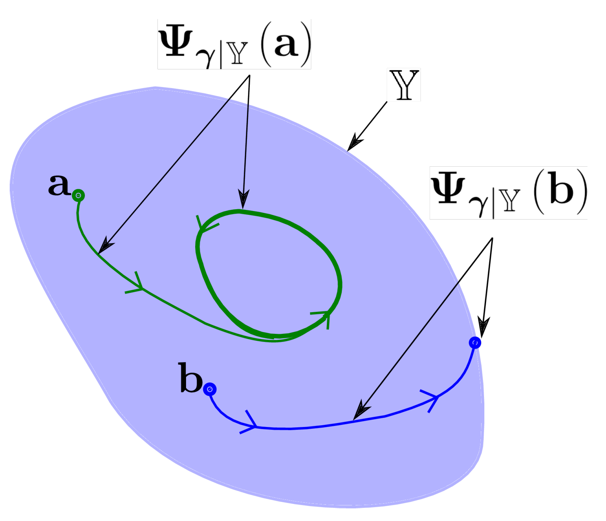
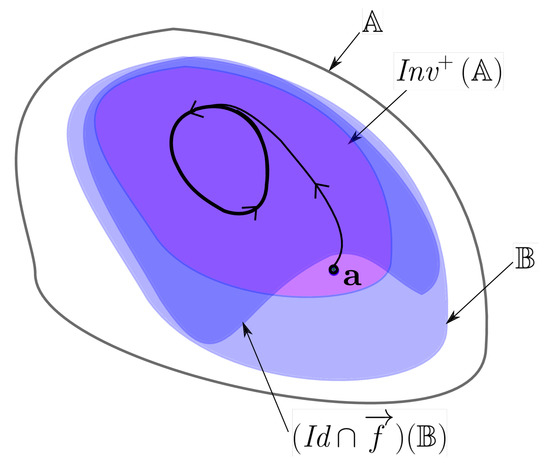
This notion is illustrated by Figure 4 where two trajectories starting from $\mathbf{a}$ and $\mathbf{b}$ are represented. The path ${\Psi }_{\mathit{\gamma }|\mathbb{Y}}\left(\mathbf{a}\right)$ contains a limit cycle, whereas ${\Psi }_{\mathit{\gamma }|\mathbb{Y}}\left(\mathbf{b}\right)$ stops at the boundary of $\mathbb{Y}$.

Figure 4. Illustration of the definition of a path inside a region.

5.3. Cover and Automorphism

In this section, we define the automorphism $\overrightarrow{f}$ that we will use to solve our problems involving invariant sets. It will be based on the notion of cover that we now define. A cover $\mathcal{P}$ is a collection of open boxes of ${\mathbb{R}}^n$ whose union is ${\mathbb{R}}^n$. Denote by $\mathcal{P}\left(\mathbf{x}\right)$ the union of all boxes of $\mathcal{P}$ containing $\mathbf{x}$.

Proposition 6.

If $\mathbb{A}$ is closed, we have

$$\mathbf{a}\in {\mathrm{Inv}}^{+}\left(\mathbb{A}\right)\Rightarrow {\Psi }_{\mathit{\gamma }|\mathcal{P}\left(\mathbf{a}\right)}\left(\mathbf{a}\right)\subset \mathbb{A}.$$

where ${\mathit{Inv}}^{+}\left(\mathbb{A}\right)$ is the largest positive invariant set included in $\mathbb{A}$.

Proof. 

We have

$$\begin{array}{ccc}\mathbf{a}\in {\mathrm{Inv}}^{+}\left(\mathbb{A}\right)& \Rightarrow \hfill & \forall t\ge 0,{\mathit{\phi }}_{\mathit{\gamma }}\left(t,\mathbf{a}\right)\in \mathbb{A}\hfill \\ & \Rightarrow \hfill & \forall t\ge 0,{\mathit{\phi }}_{\mathit{\gamma }|\mathcal{P}\left(\mathbf{a}\right)}\left(t,\mathbf{a}\right)\in \mathbb{A}\hfill \\ & \Rightarrow \hfill & {\Psi }_{\mathit{\gamma }|\mathcal{P}\left(\mathbf{a}\right)}\left(\mathbf{a}\right)\subset \mathbb{A}\hfill \end{array}$$

□

Theorem 2.

Consider the system $\mathcal{S}:\dot{\mathbf{x}}\left(t\right)=\mathit{\gamma }\left(\mathbf{x}\left(t\right)\right)$, a closed set $\mathbb{A}$, and a cover $\mathcal{P}$ of the state space. The set-valued function defined by

$$\begin{array}{ccc}\overrightarrow{f}\left(\mathbb{A}\right)& =& \left\{\mathbf{x}|{\Psi }_{\mathit{\gamma }|\mathcal{P}\left(\mathbf{x}\right)}\left(\mathbf{x}\right)\subset \mathbb{A}\right\}\end{array}$$

(27)

is an automorphism. We call $\overrightarrow{f}\left(\mathbb{A}\right)$ the forward Eulerian predictor, since it predicts where the state will go for one step. Now, the step is not temporal (as for Lagrangian predictors) but spacial and related to the cover $\mathcal{P}$.

Proof. 

First, note that we have $\overrightarrow{f}\left({\mathbb{R}}^n\right)={\mathbb{R}}^n$. Moreover,

$$\begin{array}{ccc}\overrightarrow{f}\left(\mathbb{A}\cap \mathbb{B}\right)& =& \left\{\mathbf{x}|{\Psi }_{\mathit{\gamma }|\mathcal{P}\left(\mathbf{x}\right)}\left(\mathbf{x}\right)\subset \mathbb{A}\cap \mathbb{B}\right\}\hfill \\ & =& \left\{\mathbf{x}|\left({\Psi }_{\mathit{\gamma }|\mathcal{P}\left(\mathbf{x}\right)}\left(\mathbf{x}\right)\subset \mathbb{A}\right)\right.\hfill \\ & & \mathrm{and}\left.\left({\Psi }_{\mathit{\gamma }|\mathcal{P}\left(\mathbf{x}\right)}\left(\mathbf{x}\right)\subset \mathbb{B}\right)\right\}\hfill \\ & =& \left\{\mathbf{x}|{\Psi }_{\mathit{\gamma }|\mathcal{P}\left(\mathbf{x}\right)}\left(\mathbf{x}\right)\subset \mathbb{A}\right\}\hfill \\ & & \cap \left\{\mathbf{x}|{\Psi }_{\mathit{\gamma }|\mathcal{P}\left(\mathbf{x}\right)}\left(\mathbf{x}\right)\subset \mathbb{B}\right\}\hfill \\ & =& \overrightarrow{f}\left(\mathbb{A}\right)\cap \overrightarrow{f}\left(\mathbb{B}\right).\hfill \end{array}$$

(28)

□

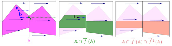
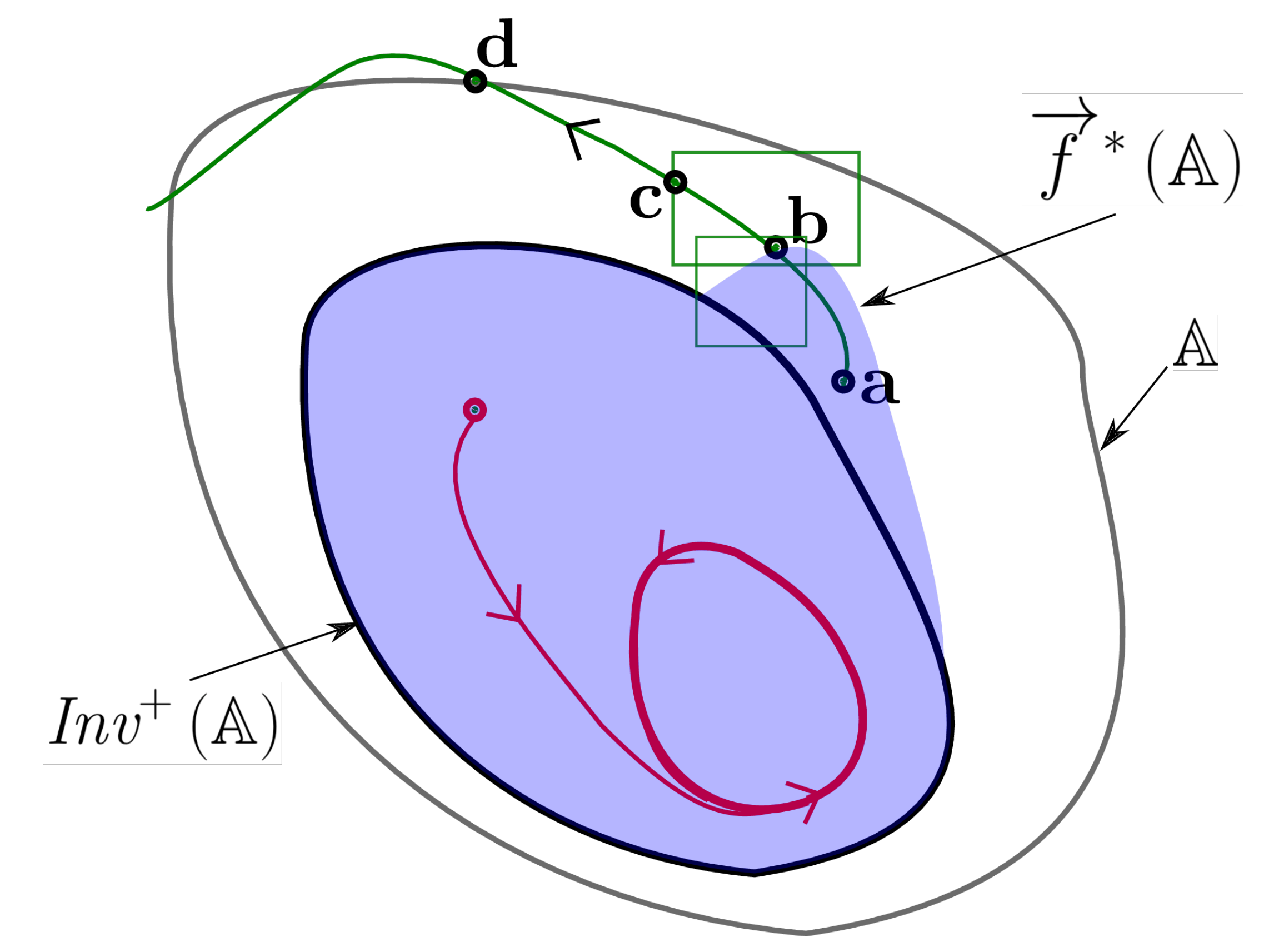
This is illustrated by Figure 5 in the case where $\mathit{\gamma }\left(\mathbf{x}\right)$, represented by its blue arrow vector field, is constant and oriented to the right. The polygonal set on the first sub-figure represents $\mathbb{A}$. In this figure, the cover is made with two boxes, which are open and overlap (just a little) on their boundaries. Now, this overlapping is not represented for the sake of clarity.

Figure 5. Forward Eulerian predictor $\overrightarrow{f}\left(\mathbb{A}\right)$ eliminating points that will escape from $\mathbb{A}$.

In the figure $\mathbf{a}\in \mathbb{A}$, $\mathcal{P}\left(\mathbf{a}\right)$ is made with a single box (the left one). The set ${\Psi }_{\mathit{\gamma }|\mathcal{P}\left(\mathbf{a}\right)}\left(\mathbf{a}\right)$ is represented by the blue dotted segment starting from $\mathbf{a}$. Since ${\Psi }_{\mathit{\gamma }|\mathcal{P}\left(\mathbf{a}\right)}\left(\mathbf{a}\right)$ is not a subset of $\mathbb{A}$, $\mathbf{a}\notin \overrightarrow{f}\left(\mathbb{A}\right)$. It means from Proposition 6 that $\mathbf{a}\notin {\mathrm{Inv}}^{+}\left(\mathbb{A}\right)$, and this is why it can be removed. We have $\mathbf{b}\in \mathbb{A}$ and ${\Psi }_{\mathit{\gamma }|\mathcal{P}\left(\mathbf{b}\right)}\left(\mathbf{b}\right)$ is the blue dotted segment starting from $\mathbf{b}$. Since ${\Psi }_{\mathit{\gamma }|\mathcal{P}\left(\mathbf{b}\right)}\left(\mathbf{b}\right)\subset \mathbb{A}$, we have $\mathbf{b}\in \overrightarrow{f}\left(\mathbb{A}\right)$. For point $\mathbf{c}\in \mathbb{A}$, the set $\mathcal{P}\left(\mathbf{c}\right)$ is made with the two boxes, instead of one for $\mathcal{P}\left(\mathbf{a}\right)$ and $\mathcal{P}\left(\mathbf{b}\right)$. As a result, ${\Psi }_{\mathit{\gamma }|\mathcal{P}\left(\mathbf{c}\right)}\left(\mathbf{c}\right)$, the left dotted green segment is not a subset of $\mathbb{A}$. Thus, $\mathbf{c}\notin \overrightarrow{f}\left(\mathbb{A}\right)$. Since $\mathbf{c}\in {\Psi }_{\mathit{\gamma }|\mathcal{P}\left(\mathbf{b}\right)}\left(\mathbf{b}\right)$ and $\mathbf{c}\notin \overrightarrow{f}\left(\mathbb{A}\right)$, we conclude that ${\Psi }_{\mathit{\gamma }|\mathcal{P}\left(\mathbf{b}\right)}\left(\mathbf{b}\right)$ is not inside $\mathbb{A}\cap \overrightarrow{f}\left(\mathbb{A}\right)$. Thus, $\mathbf{b}\notin \mathbb{A}\cap \overrightarrow{f}\left(\mathbb{A}\right)\cap {\overrightarrow{f}}^2\left(\mathbb{A}\right)$. It is eliminated, since it cannot be an element of ${\mathrm{Inv}}^{+}\left(\mathbb{A}\right)$.

5.4. Invariant Set

In this section, we now show that the automorphism is linked to invariant sets by a Kleene star operator. More precisely, we will show that ${\mathrm{Inv}}^{+}\left(\mathbb{A}\right)={\overrightarrow{f}}^{\ast }\left(\mathbb{A}\right).$ As a consequence, an interval evaluation of ${\overrightarrow{f}}^{\ast }\left(\mathbb{A}\right)$ will allow us to have an inner and an outer approximation of an invariant set ${\mathrm{Inv}}^{+}\left(\mathbb{A}\right)$.

Theorem 3.

The set ${\overrightarrow{f}}^{\ast }\left(\mathbb{A}\right)$ contains the greatest positive invariant subset of $\mathbb{A}$, i.e.,

$${\mathit{Inv}}^{+}\left(\mathbb{A}\right)\subset {\overrightarrow{f}}^{\ast }\left(\mathbb{A}\right).$$

(29)

Proof. 

The proof is by contradiction. Assume that (6) is false. Thus, there exists the largest integer i such that ${\mathrm{Inv}}^{+}\left(\mathbb{A}\right)\subset \mathbb{B}={(\mathrm{Id}\cap \overrightarrow{f})}^i\left(\mathbb{A}\right)$. Equivalently, there exists $\mathbf{a}$ (see Figure 6) such that

$$\left\{\begin{array}{ccc}\left(\mathrm{i}\right)& & \mathbf{a}\in \mathbb{B}\hfill \\ \left(\mathrm{ii}\right)& & \mathbf{a}\notin \left(\mathrm{Id}\cap \overrightarrow{f}\right)\left(\mathbb{B}\right)\hfill \\ \left(\mathrm{iii}\right)& & \mathbf{a}\in {\mathrm{Inv}}^{+}\left(\mathbb{B}\right)\hfill \end{array}\right.$$

(30)

now

$$\left(\mathrm{Id}\cap \overrightarrow{f}\right)\left(\mathbb{B}\right)=\left\{\mathbf{x}\in \mathbb{B}|{\Psi }_{\mathit{\gamma }|\mathcal{P}\left(\mathbf{x}\right)}\left(\mathbf{x}\right)\subset \mathbb{B}\right\},$$

(31)

thus

$$\left\{\begin{array}{ccc}\mathbf{a}\in {\mathrm{Inv}}^{+}\left(\mathbb{B}\right)& & (\mathrm{see} (30,\mathrm{iii}\left)\right)\hfill \\ {\Psi }_{\mathit{\gamma }|\mathcal{P}\left(\mathbf{a}\right)}\left(\mathbf{a}\right)\not\subset \mathbb{B}& & (\sin \mathrm{ce} (30,\mathrm{ii}\left)\right)\hfill \end{array}\right.$$

(32)

which is inconsistent with Proposition 6. □

Figure 6. An inconsistent situation that can never occur where $\mathbf{a}\in {\mathrm{Inv}}^{+}\left(\mathbb{A}\right)\mathrm{but}\mathbf{a}\notin {\overrightarrow{f}}^{\ast }\left(\mathbb{A}\right)$.

Theorem 4.

We have

$${\overrightarrow{f}}^{\ast }\left(\mathbb{A}\right)\subset {\mathit{Inv}}^{+}\left(\mathbb{A}\right).$$

(33)

Proof. 

The proof is by contradiction, i.e., we assume that ${\overrightarrow{f}}^{\ast }\left(\mathbb{A}\right)\not\subset {\mathrm{Inv}}^{+}\left(\mathbb{A}\right)$. In such a case, there exists $\mathbf{a}\in {\overrightarrow{f}}^{\ast }\left(\mathbb{A}\right),$ which is not in ${\mathrm{Inv}}^{+}\left(\mathbb{A}\right)$, as illustrated by Figure 7. For such a point $\mathbf{a}$, the trajectory ${\mathit{\phi }}_{\mathit{\gamma }}(t,\mathbf{a}),t\ge 0$ leaves ${\overrightarrow{f}}^{\ast }\left(\mathbb{A}\right)$ at the point $\mathbf{b}={\mathit{\phi }}_{\mathit{\gamma }}(t_b,\mathbf{a})$ for some $t_b>0$ and then leaves $\mathbb{A}$ at point $\mathbf{d}$. In the figure, the set ${\Psi }_{\mathit{\gamma }|\mathcal{P}\left(\mathbf{b}\right)\cap \mathbb{A}}\left(\mathbf{b}\right)$ corresponds to the trajectory between $\mathbf{b}$ and $\mathbf{c}$. Therefore, we can write

$$\begin{array}{ccccc}\left(i\right)& & \mathbf{b}& \in & \mathrm{boundary}\left({\overrightarrow{f}}^{\ast }\left(\mathbb{A}\right)\right)\\ \left(ii\right)& & \mathbf{b}& \notin & \left(\mathrm{Id}\cap \overrightarrow{f}\right)\left({\overrightarrow{f}}^{\ast }\left(\mathbb{A}\right)\right)\end{array},$$

(34)

however, also, there exists a neighborhood ${\mathcal{V}}_{\mathbf{b}}$ of $\mathbf{b}$ such that

$$\forall {\mathbf{b}}^{\prime }\in {\mathcal{V}}_{\mathbf{b}},{\mathbf{b}}^{\prime }\notin \underset{={\overrightarrow{f}}^{\ast }\left(\mathbb{A}\right)}{\underbrace{\left(\mathrm{Id}\cap \overrightarrow{f}\right)\left({\overrightarrow{f}}^{\ast }\left(\mathbb{A}\right)\right)}}$$

(35)

which is inconsistent with (34, (i)). □

Figure 7. An impossible situation where $\mathbf{a}\notin {\mathrm{Inv}}^{+}\left(\mathbb{A}\right)\mathrm{but}\mathbf{a}\in {\overrightarrow{f}}^{\ast }\left(\mathbb{A}\right)$ that is used in the proof of Theorem 4.

Corollary 1.

The set-valued function

$$\begin{array}{ccc}\overleftarrow{f}\left(\mathbb{A}\right)& =& \left\{\mathbf{x}|\Psi {}_{-\mathit{\gamma }|\mathcal{P}\left(\mathbf{x}\right)}\left(\mathbf{x}\right)\subset \mathbb{A}\right\}\end{array}$$

(36)

is an automorphism. Moreover, ${\overleftarrow{f}}^{\ast }\left(\mathbb{A}\right)$ corresponds to the greatest negative invariant subset of $\mathbb{A}$, i.e.,

$${\overleftarrow{f}}^{\ast }\left(\mathbb{A}\right)={\mathit{Inv}}^{+}\left(-\mathit{\gamma },\mathbb{A}\right)\stackrel{\left(3\right)}{=}\left\{\mathbf{a}|\forall t\ge 0,{\mathit{\phi }}_{\mathit{\gamma }}\left(-t,\mathbf{a}\right)\in \mathbb{A}\right\}.$$

(37)

6. Test Cases

We consider here several test cases in order to illustrate the principle and the efficiency of our approach. We can note that our method is limited to small-dimension systems because of the exponential complexity of the algorithm w.r.t. the dimension. This is indeed the case for all safe methods dealing with non-convex solution sets.

6.1. Negative Invariant

We consider here a problem treated in [30] involving the Van der Pol system:

$$\left\{\begin{array}{ccc}{\dot{x}}_1\hfill & =\hfill & x_2\hfill \\ {\dot{x}}_2\hfill & =\hfill & \left(1-x_1^2\right)·x_2-x_1.\hfill \end{array}\right.$$

(38)

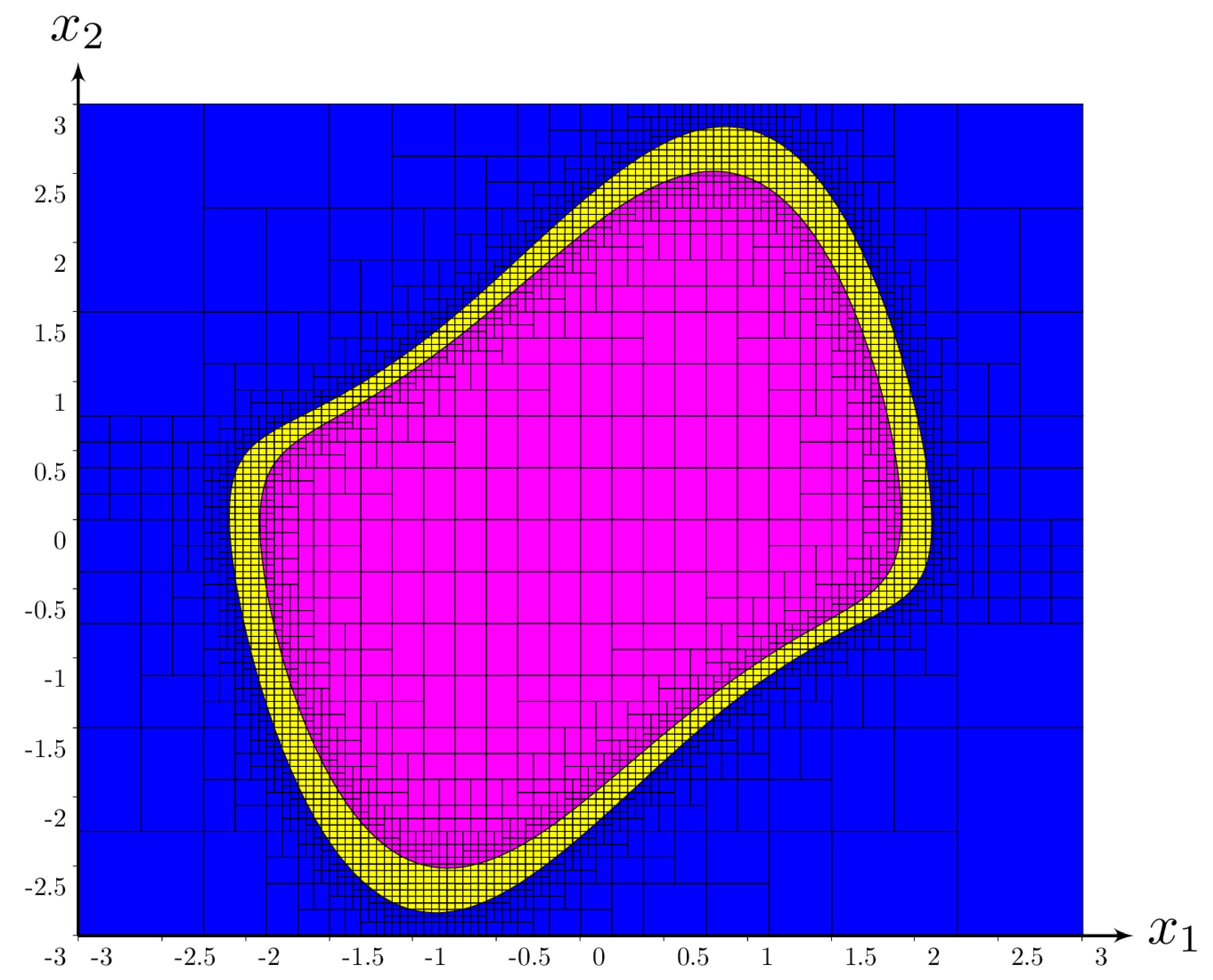
Let us take for initial box $\mathbb{A}=\left[-3,3\right]\times \left[-3,3\right]$. To compute the greatest negative invariant subset $\mathbb{X}$ of $\mathbb{A}$, we compute $\left[{\overleftarrow{f}}^{\ast }\right]\left(\mathbb{A}\right)$, where $\overleftarrow{f}$ is the automorphism defined by 36 and $\left[{\overleftarrow{f}}^{\ast }\right]$ is a machine interval enclosure for ${\overleftarrow{f}}^{\ast }$ (see Equation (21)). The resulting approximation is illustrated by Figure 8, which is obtained in less than 5 s on a standard laptop (all the computations were performed on an Intel i5-3320M@2.6 GHz with 8 GB of RAM). The magenta part corresponds to the inner approximation ${\mathbb{X}}^{-}$ of $\mathbb{X}$. From (19), we know that ${\mathbb{X}}^{-}$ (magenta) is a negative invariant set. The outer approximation ${\mathbb{X}}^{+}$ corresponds to the union of the yellow and the magenta zones. Note that ${\mathbb{X}}^{+}$ may not be negative invariant.

Figure 8. Approximation of the greatest negative invariant set included in the frame box $\mathbb{A}$.

6.2. Forward Reach Set

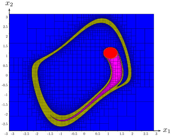
Given the system (38), the forward reach set [48] of a set $\mathbb{A}$ is defined by

$$\begin{array}{ccc}\mathrm{Fwd}\left(\mathbb{A}\right)& =& \left\{\mathbf{x}|\exists t\ge 0,{\mathit{\phi }}_{\mathit{\gamma }}\left(-t,\mathbf{x}\right)\in \mathbb{A}\right\}\\ & =& \overline{\left\{\mathbf{x}|\forall t\ge 0,{\mathit{\phi }}_{\mathit{\gamma }}\left(-t,\mathbf{x}\right)\in \overline{\mathbb{A}}\right\}}\\ & \stackrel{\left(37\right)}{=}& \overline{{\overleftarrow{f}}^{\ast }\left(\overline{\mathbb{A}}\right)}\end{array}$$

(39)

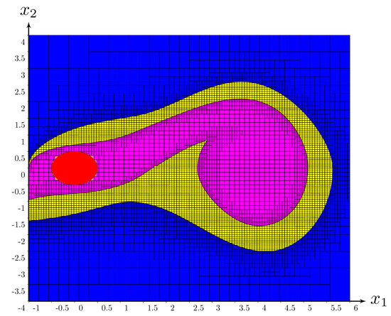
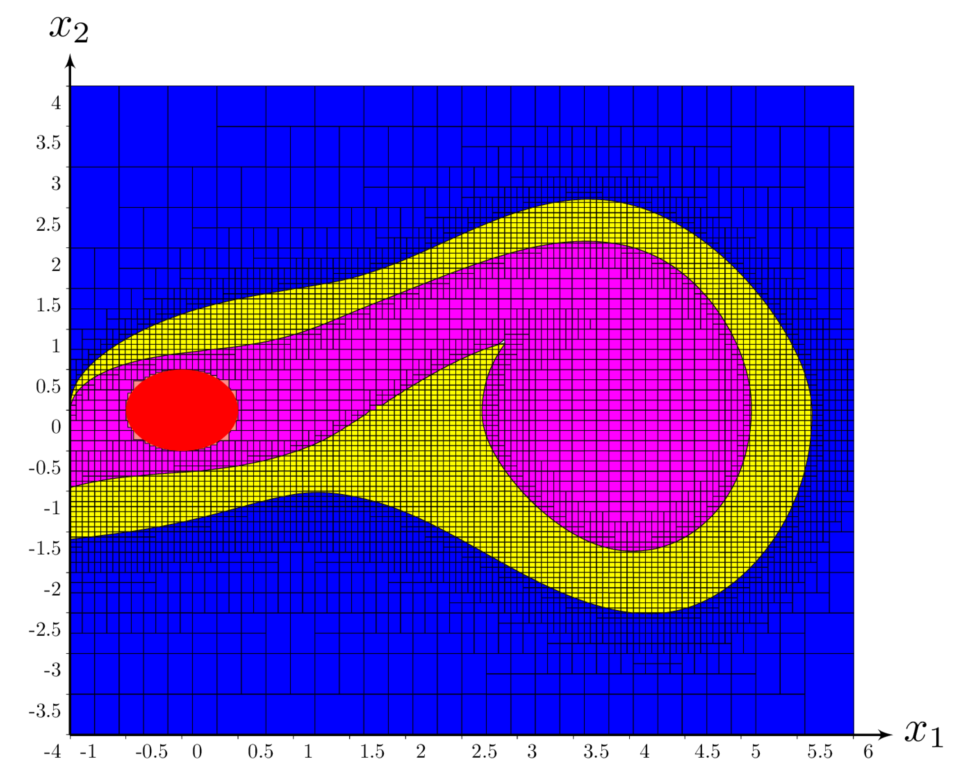
We obtain in less than 4 s, with $\mathbb{A}=\left\{\left(x_1,x_2\right)\in {\mathbb{R}}^2|{\left(x_1-1.2\right)}^2+{\left(x_2-1\right)}^2\le 0.3{}^2\right\}$, the approximation illustrated by Figure 9. The frame box is $\left[-3,3\right]\times \left[-3,3\right].$ Note that we were able to get a non-empty inner approximation of Fwd$\left(\mathbb{A}\right)$ that was not possible with existing interval base methods such as [49]. Similar results could have been obtained using flow* [50], but to have the guarantee to enclose the whole trajectory, we need to deal with an infinite horizon, whereas the Taylor-based method (used in Flow*) is devoted to predict the trajectory for a limited time horizon.

Figure 9. Forward reach set associated with the red disk $\mathbb{A}$ for an infinite time horizon.

6.3. Backward Reach Set

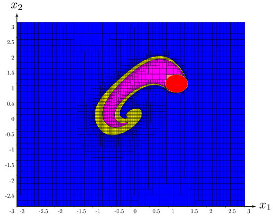
Given a set $\mathbb{A}$, the backward reach set is defined by

$$\begin{array}{ccc}\mathrm{Bwd}\left(\mathbb{A}\right)& =& \left\{\mathbf{x}|\exists t\ge 0,{\mathit{\phi }}_{\mathit{\gamma }}\left(t,\mathbf{x}\right)\in \mathbb{A}\right\}\\ & =& \overline{\left\{\mathbf{x}|\forall t\ge 0,{\mathit{\phi }}_{\mathit{\gamma }}\left(t,\mathbf{x}\right)\in \overline{\mathbb{A}}\right\}}\\ & \stackrel{\left(23\right)}{=}& \overline{{\overrightarrow{f}}^{\ast }\left(\overline{\mathbb{A}}\right)}\end{array}$$

(40)

For the system (38), we get in less than 4 s the approximation of $\mathrm{Bwd}\left(\mathbb{A}\right)$, as illustrated by Figure 10. The frame box is $\left[-3,3\right]\times \left[-3,3\right]$.

Figure 10. Forward reach set associated with the red disk $\mathbb{A}$.

6.4. Control Forward Reach Set

Consider the system:

$$\mathcal{S}:\dot{\mathbf{x}}\left(t\right)=\mathit{\gamma }\left(\mathbf{x}\left(t\right),u\right),u\in \left\{u_0,u_1\right\}$$

(41)

where u is the control that can be chosen asynchronously inside the set $\left\{0,1\right\}$. Given an initial state set $\mathbb{A}$, we want to compute the set $\mathbb{X}$ of all states that can be reached from $\mathbb{A}$ [51]. We have

$$\begin{array}{ccc}\mathbb{X}& =& {\left({\mathrm{Forw}}_{u=u_1}\circ {\mathrm{Forw}}_{u=u_0}\right)}^{\infty }\left(\mathbb{A}\right)\end{array}.$$

(42)

Equivalently, $\mathbb{X}$ can be defined as the limit of the sequence

$$\begin{array}{ccc}\mathbb{X}\left(k+1\right)& =& {\mathrm{Forw}}_{u=u_1}\left({\mathrm{Forw}}_{u=u_0}\left(\mathbb{X}\left(k\right)\right)\right)\\ \mathbb{X}\left(0\right)& =& \mathbb{A}\end{array},$$

(43)

thus,

$$\begin{array}{ccc}\overline{\mathbb{X}}\left(k+1\right)& =& {\overleftarrow{f_1}}^{\ast }\left(\overline{{\mathrm{Forw}}_{u=u_0}\left(\mathbb{X}\left(k\right)\right)}\right)\\ & =& {\overleftarrow{f_1}}^{\ast }\left(\overline{\overline{{\overleftarrow{f_0}}^{\ast }\left(\overline{\mathbb{X}\left(k\right)}\right)}}\right)\\ & =& {\overleftarrow{f_1}}^{\ast }\circ {\overleftarrow{f_0}}^{\ast }\left(\overline{\mathbb{X}\left(k\right)}\right).\end{array}$$

(44)

Therefore, we have:

$$\overline{\mathbb{X}}=\underset{k\to \infty }{lim}\overline{\mathbb{X}}\left(k\right)={\left({\overleftarrow{f_1}}^{\ast }\circ {\overleftarrow{f_0}}^{\ast }\right)}^{\ast }\left(\overline{\mathbb{A}}\right)={\left(\overleftarrow{f_1}\circ \overleftarrow{f_0}\right)}^{\ast }\left(\overline{\mathbb{A}}\right)$$

(45)

and finally,

$$\mathbb{X}=\overline{{\left(\overleftarrow{f_1}\circ \overleftarrow{f_0}\right)}^{\ast }\left(\overline{\mathbb{A}}\right)}.$$

(46)

We consider as an example the car on the hill system [47] where

$$\left\{\begin{array}{cc}{\dot{x}}_1=\hfill & x_2\hfill \\ {\dot{x}}_2=\hfill & -9.81sin(0.55sin\left(1.2x_1\right)-0.6sin\left(1.1x_1\right))\hfill \\ & -0.7x_2+u\hfill \end{array}\right.$$

with the set $\mathbb{A}=\left\{(x_1,x_2)\in {\mathbb{R}}^2|x_1^2+x_2^2\le 0.5{}^2\right\}$ and $u\in \{-1,1\}$. We get in less than 10 s the approximation illustrated by Figure 11, where the frame box is $[-1,6]\times [-4,4]$.

Figure 11. Inner and outer approximation of the control forward reach set.

6.5. Minimal Robust Positive Invariant Set

The example is a continuous-time version of the example taken from [52]. We consider the system described by

$$\left\{\begin{array}{cc}{\dot{x}}_1=\hfill & 0.2x_1+0.2x_2-x_1\hfill \\ {\dot{x}}_2=\hfill & -0.2x_1+0.5x_2+\omega -x_1\hfill \end{array}\right.$$

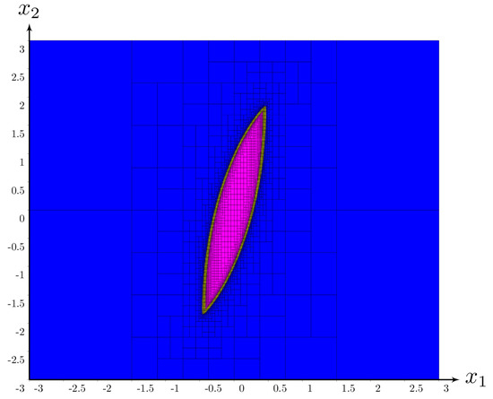
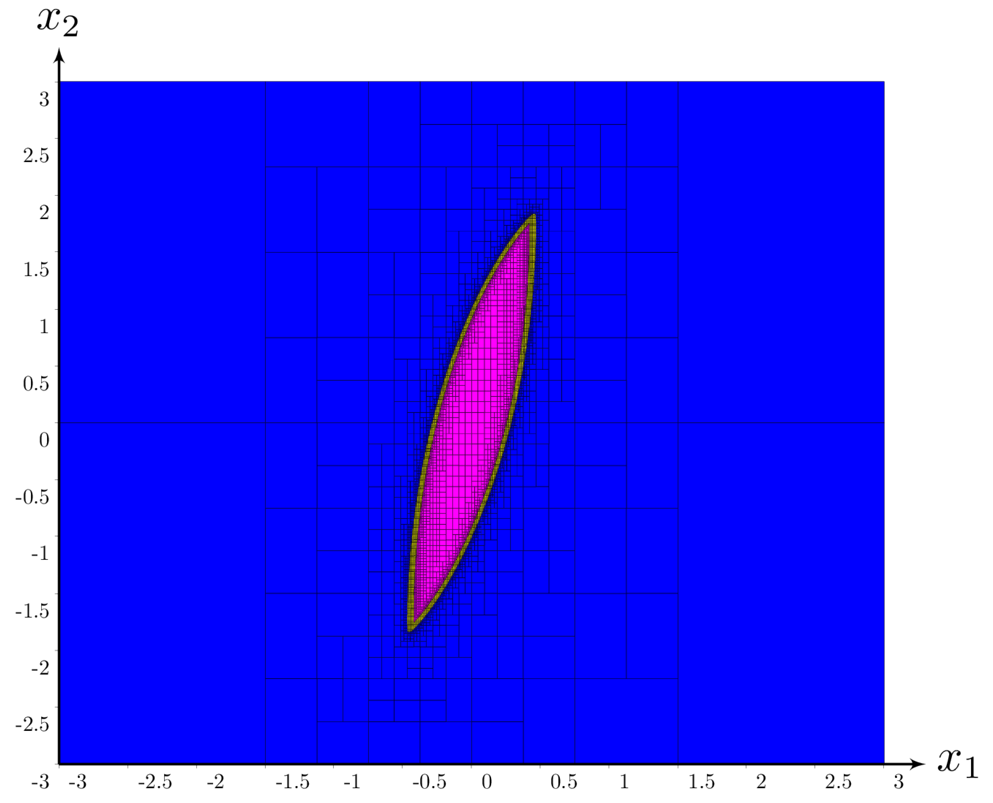
where $\omega \in \left[\omega \right]=\left[-1,1\right]$ is the perturbation. The system has the form $\dot{\mathbf{x}}\left(t\right)=\mathit{\gamma }\left(\mathbf{x}\left(t\right),\omega \right)$. We want to compute the smallest set $\mathbb{X}$ containing $\mathbf{0}$ such that the system cannot escape. This set corresponds to the minimal robust positively invariant set [53] and is known to be difficult to compute. Moreover, no method exists in the literature to get a guaranteed inner approximation for nonlinear continuous-time systems. Now, this problem is similar to the previous one except that the control u is now replaced by a perturbation $\omega$, and we can use the same method. In 2 s, we obtain the approximation illustrated by Figure 12 where the frame box is $\left[-3,3\right]\times \left[-3,3\right]$.

Figure 12. Approximation of the smallest positive invariant set containing $\mathbf{0}$.

6.6. Path Planning

Given the system (38) and three sets

$$\left\{\begin{array}{cc}\mathbb{A}:\hfill & {\left(x_1-0.8\right)}^2+{\left(x_2-1.3\right)}^2\le {\left(0.4\right)}^2\hfill \\ \mathbb{B}:\hfill & \left[1.35,1.45\right]\times \left[-0.2,0\right]\hfill \\ \mathbb{C}:\hfill & \left[0.74,1.2\right]\times \left[-1.5,-1.06\right]\hfill \end{array}\right..$$

Let us find the set $\mathbb{X}$ of all points corresponding to a path that starts from $\mathbb{A}$, avoids $\mathbb{B}$, and reaches $\mathbb{C}$. It corresponds to a path planning problem [54,55] for which interval analysis has been shown to be particularly efficient [56,57,58]. We have

$$\begin{array}{ccc}\mathbb{X}& =& {\mathrm{Forw}}_{\mathit{\gamma }|\overline{\mathbb{B}}}\left(\mathbb{A}\right)\cap {\mathrm{Back}}_{\mathit{\gamma }|\overline{\mathbb{B}}}\left(\mathbb{C}\right)\\ & =& \overline{\overleftarrow{f_{\mathit{\gamma }|{\overline{\mathbb{B}}}^{\ast }}}\left(\overline{\mathbb{A}}\right)}\cap \overline{\overrightarrow{f_{\mathit{\gamma }|{\overline{\mathbb{B}}}^{\ast }}}\left(\overline{\mathbb{C}}\right)}\end{array}$$

(47)

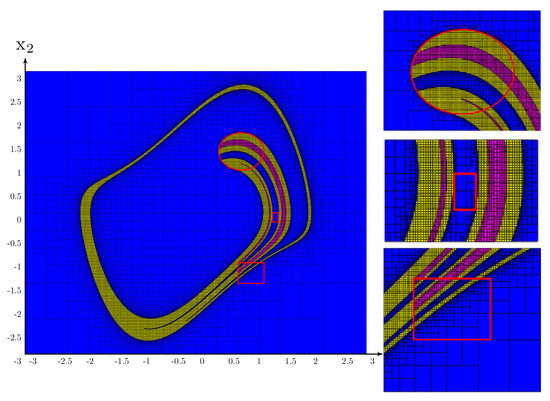
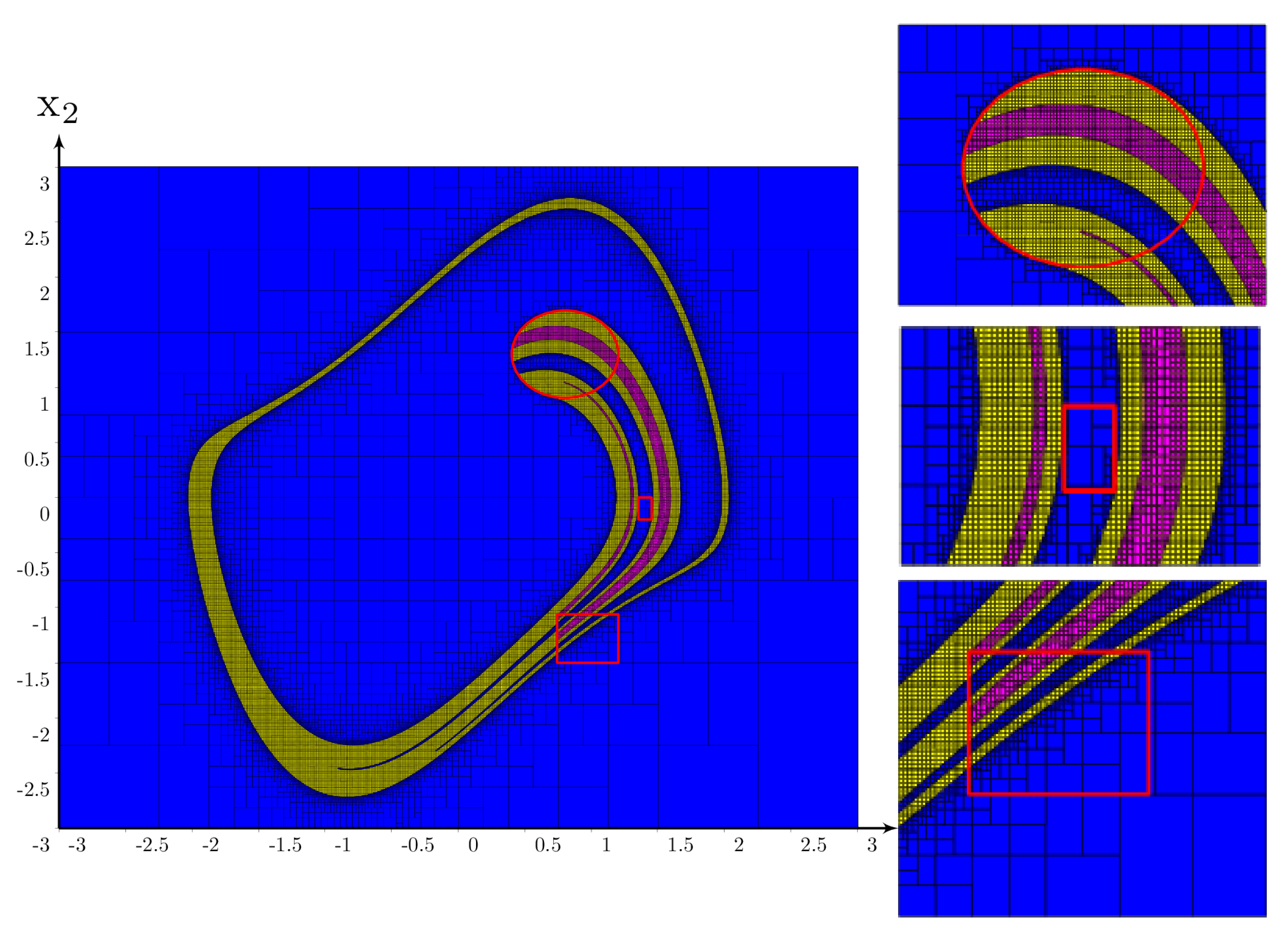
and thus our methodology applies. The result, depicted on Figure 13 left, was obtained in less than 38 s for a search box $[-3,3]\times [-3,3]$. The three images on the right show on several zooms around $\mathbb{A},\mathbb{B},\mathbb{C}$ that a non-empty inner approximation was obtained, which was not possible with existing solvers.

Figure 13. Paths starting from $\mathbb{A}$, avoiding $\mathbb{B}$, and reaching $\mathbb{C}$.

7. Conclusions

In this paper, we have proposed a new approach to compute invariant sets of continuous-time dynamical systems. Our contributions are the following:

• A link between Kleene algebra and invariant sets. This allowed us to derive a simple fixed point method able to compute guaranteed inner and outer approximations of invariant sets.
• The treatment of toy examples for which no other existing approach is able to deal with.

The approach uses the fact that a suited automorphism has been found for a dynamical system described by a deterministic state equation.

Moreover, our formalism allowed us to compute sets that can be defined as combinations (intersection, union, complementary, image by automorphism) of invariant sets. This combination can be interpreted as a first step toward what could be called an invariant algebra, i.e., an algebra the atoms of which are positive invariant sets of dynamical systems. This algebra transforms a complex problem such as the reach and avoid problem without developing a complex algorithm with properties that are difficult to analyze. Instead, our algebra yields a simple expression operating in our invariant algebra.

Our approach can directly be extended to discrete time system and the algorithm, based on a formal expression, remains unchanged. Only atoms (i.e., the automorphisms) have to be adapted. For a discrete time system of the form $\mathbf{x}(k+1)=\mathit{\gamma }\left(\mathbf{x}\right(k\left)\right)$, the automorphism is even simpler, since it could be $\mathbb{X}\mapsto \mathit{\gamma }\left(\mathbb{X}\right)=\left\{\mathbf{y}\right|\exists \mathbf{x}\in \mathbb{X},\mathbf{y}=\mathit{\gamma }\left(\mathbf{x}\right)\}$. Thus, we get an approach similar to that proposed in [59] where the set invariance is used to prove properties of discrete-time dynamical systems in a context of temporal logic.

In our approach, we have chosen a structure that is a Kleene algebra. It captures many properties we have when we deal with invariant sets. Now, some properties are forgotten by the Kleene algebra. For instance, for our continuous-time systems, we have the property $\overrightarrow{f}\circ \overrightarrow{f}\supset \overrightarrow{f}$. From this property, we may get some other simplifications that could be used to increase the efficiency of the resolution.

The Python code with all examples is made available at (1 March 2022): https://www.ensta-bretagne.fr/lemezo/pyinvariant/pyinvariant.html.

References

- Jaulin, L. Automation for Robotics; ISTE: Eugene, OR, USA, 2015. [Google Scholar]
- Jaulin, L. Mobile Robotics; ISTE: Eugene, OR, USA, 2015. [Google Scholar]
- Blanchini, F.; Miani, S. Set-Theoretic Methods in Control; Springer Science & Business Media: Berlin/Heidelberg, Germany, 2007. [Google Scholar]
- Esik, Z.; Fahrenberg, U.; Legay, A.; Quaas, K. An Algebraic Approach to Energy Problems II, The Algebra of Energy Functions. Acta Cybern. 2017, 23, 229–268. [Google Scholar] [CrossRef] [Scilit]
- Wan, J.; Vehi, J.; Luo, N. A numerical approach to design control invariant sets for constrained nonlinear discrete-time systems with guaranteed optimality. J. Glob. Optim. 2009, 44, 395–407. [Google Scholar] [CrossRef] [Scilit]
- Olaru, S.; Dona, J.D.; Seron, M.; Stoican, F. Positive invariant sets for fault tolerant multisensor control schemes. Int. J. Control 2010, 83, 2622–2640. [Google Scholar] [CrossRef] [Scilit]
- Althoff, D.; Althoff, M.; Scherer, S. Online Safety Verification of Trajectories for Unmanned Flight with Offline Computed Robust Invariant Sets. In Proceedings of the IEEE/RSJ International Conference on Intelligent Robots and Systems, Hamburg, Germany, 28 September–2 October 2015. [Google Scholar]
- Asarin, E.; Dang, T.; Maler, O. The d/dt tool for verification of hybrid systems. In Proceedings of the International Conference on Computer Aided Verification, Los Angeles, CA, USA, 21–24 July 2002; pp. 365–370. [Google Scholar]
- Tabuada, P. Verification and Control of Hybrid Systems: A Symbolic Approach; Springer: Berlin/Heidelberg, Germany, 2009. [Google Scholar]
- Mitchell, I. Comparing forward and backward reachability as tools for safety analysis. In Hybrid Systems: Computation and Control; Bemporad, A., Bicchi, A., Buttazzo, G., Eds.; Springer: Berlin/Heidelberg, Germany, 2007; pp. 428–443. [Google Scholar]
- Tahir, F.; Jaimoukha, M. Low-Complexity Polytopic Invariant Sets for Linear Systems Subject to Norm-Bounded Uncertainty. IEEE Trans. Autom. Control 2015, 60, 1416–1421. [Google Scholar] [CrossRef] [Scilit]
- Roux, P.; Jobredeaux, R.; Garoche, P.; Feron, E. A generic ellipsoid abstract domain for linear time invariant systems. In Proceedings of the Hybrid Systems: Computation and Control, HSCC’12, Beijing, China, 17–19 April 2012; pp. 105–114. [Google Scholar]
- Bertsekas, D. Infinite-time reachability of state-space regions by using feedback Control. IEEE Trans. Autom. Control 1972, 17, 604–613. [Google Scholar] [CrossRef] [Scilit]
- Athanasopoulos, N.; Smpoukis, K.; Jungers, R. Invariant Sets Analysis for Constrained Switching Systems. IEEE Control Syst. Lett. 2017, 1, 256–261. [Google Scholar] [CrossRef] [Scilit]
- Allamigeon, X.; Gaubert, S.; Goubault, E.; Putot, S.; Stott, N. A fast method to compute disjunctive quadratic invariants of numerical programs. Acm Trans. Embed. Comput. Syst. 2017, 6, 1–19. [Google Scholar] [CrossRef] [Scilit]
- Guernic, C.L.; Girard, A. Reachability analysis of linear systems using support functions. Nonlinear Anal. 2009, 4, 250–262. [Google Scholar] [CrossRef] [Scilit]
- Ghorbal, K.; Goubault, E.; Putot, S. A logical product approach to zonotope intersection. In Computer Aided Verification, CAV 2010; Touili, T., Cook, B., Jackson, P., Eds.; Springer: Edinburgh, UK, 2010. [Google Scholar]
- Asarin, E.; Dang, T.; Girard, A. Hybridization methods for the analysis of non-linear systems. Acta Inform. 2007, 7, 451–476. [Google Scholar] [CrossRef] [Scilit]
- Girard, A. Computation and stability analysis of limit cycles in piecewise linear hybrid systems. In Proceedings of the 1st IFAC Conference on Analysis and Design of Hybrid Systems, St Malo, France, 16–18 June 2003; pp. 181–186. [Google Scholar]
- Sankaranarayanan, S.; Dang, T.; Ivancic, F. Symbolic model checking of hybrid systems using template polyhedra. Tacas Lect. Notes Comput. Sci. 2008, 4963, 188–202. [Google Scholar]
- Saint-Pierre, P. Approximation of the viability kernel. Appl. Math. Optim. 1994, 29, 187–209. [Google Scholar] [CrossRef] [Scilit]
- Bobiti, R.; Lazar, M. Automated-Sampling-Based Stability Verification and DOA Estimation for Nonlinear Systems. IEEE Trans. Autom. Control 2018, 63, 3659–3674. [Google Scholar] [CrossRef] [Scilit]
- Goubault, E.; Mullier, O.; Putot, S.; Kieffer, M. Inner approximated reachability analysis. In Proceedings of the 17th International Conference on Hybrid Systems: Computation and Control, HSCC’14, Berlin, Germany, 15–17 April 2014; pp. 163–172. [Google Scholar]
- Wilczak, D.; Zgliczynski, P. Cr-Lohner algorithm. Schedae Inform. 2011, 20, 9–46. [Google Scholar]
- Goubault, E.; Putot, S. Forward Inner-Approximated Reachability of Non-Linear Continuous Systems. In Proceedings of the 20th International Conference on Hybrid Systems: Computation and Control, Pittsburgh, PA, USA, 18–20 April 2017; Association for Computing Machinery: New York, NY, USA, 2017; pp. 1–10. [Google Scholar] [CrossRef] [Scilit]
- Giesl, P.; Hafstein, S. Review on computational methods for Lyapunov functions. Discret. Contin. Dyn. Syst. 2015, 8, 2291–2331. [Google Scholar]
- Henrion, D.; Korda, M. Convex computation of the region of attraction of polynomial control systems. IEEE Trans. Autom. Control 2013, 59, 297–312. [Google Scholar] [CrossRef] [Scilit]
- Ratschan, S.; She, Z. Providing a Basin of Attraction to a Target Region of Polynomial Systems by Computation of Lyapunov-like Functions. SIAM J. Control Optim. 2010, 48, 4377–4394. [Google Scholar] [CrossRef] [Scilit]
- Oustry, A.; Tacchi, M.; Henrion, D. Inner approximations of the maximal positively invariant set for polynomial dynamical systems. IEEE Control Syst. Lett. 2019, 3, 733–738. [Google Scholar] [CrossRef] [Scilit]
- Boczko, E.; Kalies, W.; Mischaikow, K. Polygonal approximation of flows. Topol. Its Appl. 2007, 154, 2501–2520. [Google Scholar] [CrossRef] [Scilit]
- Mézo, T.L.; Jaulin, L.; Zerr, B. An interval approach to compute invariant sets. IEEE Trans. Autom. Control 2017, 62, 4236–4243. [Google Scholar] [CrossRef] [Scilit]
- Conley, C. Isolated Invariant Sets and the Morse Index; American Mathematical Society: Providence, RI, USA, 1991. [Google Scholar]
- Frehse, G. PHAVer: Algorithmic Verification of Hybrid Systems. Int. J. Softw. Tools Technol. Transf. 2008, 10, 23–48. [Google Scholar] [CrossRef] [Scilit]
- Frehse, G.; Le Guernic, C.; Donzé, A.; Cotton, S.; Ray, R.; Lebeltel, O.; Ripado, R.; Girard, A.; Dang, T.; Maler, O. SpaceEx: Scalable Verification of Hybrid Systems. In Proceedings of the 23rd International Conference on Computer Aided Verification (CAV), Snowbird, UT, USA, 14–20 July 2011. [Google Scholar]
- LaValle, S. Planning Algorithm; Cambridge University Press: Cambridge, UK, 2006. [Google Scholar]
- Kalies, W.; Mischaikow, K.; Vandervorst, R. Lattice Structures for Attractors. Found. Comput. Math. 2016, 16, 1151–1191. [Google Scholar] [CrossRef] [Scilit]
- Davey, B.A.; Priestley, H.A. Introduction to Lattices and Order; Cambridge University Press: Cambridge, UK, 2002; ISBN 0521784514. [Google Scholar]
- Monniaux, D. The pitfalls of verifying floating-point computations. Acm Trans. Program. Lang. Syst. 2008, 30, 1–12. [Google Scholar] [CrossRef] [Scilit]
- Mézo, T.L.; Jaulin, L.; Zerr, B. Bracketing the solutions of an ordinary differential equation with uncertain initial conditions. Appl. Math. Comput. 2018, 318, 70–79. [Google Scholar]
- Mézo, T.L.; Jaulin, L.; Zerr, B. Bracketing backward reach sets of a dynamical system. Int. J. Control 2019, 93, 2528–2540. [Google Scholar] [CrossRef] [Scilit]
- Kozen, D. On Kleene algebras and closed semirings. In International Symposium on Mathematical Foundations of Computer Science; Springer: Berlin/Heidelberg, Germany, 1990; pp. 26–47. [Google Scholar]
- Kozen, D. A completeness theorem for Kleene algebras and the algebra of regular events. In Proceedings of the Sixth Annual IEEE Symposium on Logic in Computer Science, LICS, Amsterdam, The Netherlands, 15–18 July 1991; pp. 214–225. [Google Scholar]
- Moore, R.E. Interval Analysis; Prentice-Hall: Englewood Cliffs, NJ, USA, 1966. [Google Scholar]
- Lhommeau, M.; Hardouin, L.; Cottenceau, B.; Jaulin, L. Interval Analysis and Dioid: Application to Robust Controller Design for Timed Event Graphs. Automatica 2004, 40, 1923–1930. [Google Scholar] [CrossRef] [Scilit]
- Rohou, S.; Jaulin, L.; Mihaylova, M.; Bars, F.L.; Veres, S. Guaranteed Computation of Robots Trajectories. Robot. Auton. Syst. 2017, 93, 76–84. [Google Scholar] [CrossRef] [Scilit]
- Monnet, D.; Ninin, J.; Jaulin, L. Computing an inner and an outer approximation of the viability kernel. Reliab. Comput. 2016, 22, 138–148. [Google Scholar]
- Lhommeau, M.; Jaulin, L.; Hardouin, L. Capture Basin Approximation using Interval Analysis. Int. J. Adapt. Control Signal Process. 2011, 25, 264–272. [Google Scholar] [CrossRef] [Scilit]
- Dang, T.; Guernic, C.L.; Maler, O. Computing reachable states for nonlinear biological models. Comput. Methods Syst. Biol. 2009, 5688, 126–141. [Google Scholar]
- Ramdani, N.; Nedialkov, N. Computing Reachable Sets for Uncertain Nonlinear Hybrid Systems using Interval Constraint Propagation Techniques. Nonlinear Anal. Hybrid Syst. 2011, 5, 149–162. [Google Scholar] [CrossRef] [Scilit]
- Chen, X. Reachability Analysis of Non-LinearHybrid Systems Using Taylor Models. Ph.D. Thesis, University of Aachen, Aachen, Germany, 2015. [Google Scholar]
- Girard, A.; Guernic, C.L.; Maler, O. Efficient computation of reachable sets of linear time-invariant systems with inputs. Hybrid Syst. Comput. Control 2006, 3927, 257–271. [Google Scholar]
- Meslem, N.; Loukkas, N.; Martinez, J. Using set invariance to design robust interval observers for discrete time linear systems. Int. J. Robust Nonlinear Control 2018, 28, 3623–3639. [Google Scholar] [CrossRef] [Scilit]
- Rakovic, S.V.; Kerrigan, E.C.; Kouramas, K.I.; Mayne, D.Q. Invariant approximations of the minimal robust positively invariant set. IEEE Trans. Autom. Control 2005, 50, 406–410. [Google Scholar] [CrossRef] [Scilit]
- Lozano-Pérez, T. Spatial Planning: A Configuration Space Approach. IEEE Trans. Comput. 1983, 32, 108–120. [Google Scholar] [CrossRef] [Scilit]
- Rungger, M.; Zamani, M. SCOTS: A Tool for the Synthesis of Symbolic Controllers. In Proceedings of the HSCC 2016, Vienna, Austria, 12–14 April 2016. [Google Scholar] [CrossRef] [Scilit]
- Jaulin, L. Path Planning Using Intervals and Graphs. Reliab. Comput. 2001, 7, 1–15. [Google Scholar] [CrossRef] [Scilit]
- Pepy, R.; Kieffer, M.; Walter, E. Reliable Robust Path Planning with Application to Mobile Robots. Int. J. Appl. Math. Comput. Sci. 2009, 19, 413–424. [Google Scholar] [CrossRef] [Scilit]
- Crépon, P.; Panchea, A.; Chapoutot, A. Reliable Motion Plannning for a Mobile Robot. In Proceedings of the IEEE International Conference on Robotic Computing, Laguna Hills, CA, USA, 31 January–2 February 2018. [Google Scholar]
- Belta, C.; Yordanov, B.; Gol, E. Formal Methods for Discrete-Time Dynamical Systems; Studies in Systems, Decision and Control; Springer International Publishing: Berlin/Heidelberg, Germany, 2017. [Google Scholar]
Publisher’s Note: MDPI stays neutral with regard to jurisdictional claims in published maps and institutional affiliations. |
© 2022 by the authors. Licensee MDPI, Basel, Switzerland. This article is an open access article distributed under the terms and conditions of the Creative Commons Attribution (CC BY) license (https://creativecommons.org/licenses/by/4.0/).