Analysis of Explainable Goal-Driven Reinforcement Learning in a Continuous Simulated Environment

Abstract

Currently, artificial intelligence is in an important period of growth. Due to the technology boom, it is now possible to solve problems that could not be resolved previously. For example, through goal-driven learning, it is possible that intelligent machines or agents may be able to perform tasks without human intervention. However, this also leads to the problem of understanding the agent’s decision making. Therefore, explainable goal-driven learning attempts to eliminate this gap. This work focuses on the adaptability of two explainability methods in continuous environments. The methods based on learning and introspection proposed a probability value for success to explain the agent’s behavior. These had already been tested in discrete environments. The continuous environment used in this study is the car-racing problem. This is a simulated car racing game that forms part of the Python Open AI Gym Library. The agents in this environment were trained with the Deep Q-Network algorithm, and in parallel the explainability methods were implemented. This research included a proposal for carrying out the adaptation and implementation of these methods in continuous states. The adaptation of the learning method produced major changes, implemented through an artificial neural network. The obtained probabilities of both methods were consistent throughout the experiments. The probability result was greater in the learning method. In terms of computational resources, the introspection method was slightly better than its counterpart.

1. Introduction

Machine learning has become widespread within the daily life of individuals. Without our realization, more and more algorithms are analyzing and learning to help us with some tasks, such as, recommending personalized movies or music [1], looking for deleted emails [2], facial recognition [3], in medicine [4], and also in autonomous vehicles [5]. Therefore, in some circumstances, it is important that the user understand what information these machine systems or robots are providing; otherwise, they would be unreliable. For example, it would not be useful to have an algorithm that recommended movies we do not like, or, also, it would be serious if a medical system made a faulty negative diagnosis during an evaluation of a patient with cancer. In this context, the role of explainable artificial intelligence is an important role since it consists of tools, techniques, and algorithms that provide the agent with the ability to explain its action to the human intuitively [6,7].

In human–agent interaction scenarios, it is possible that a non-expert user does not understand why the agent makes a specific decision. As a result, some questions may arise on the part of the user under these circumstances: why?; why not?; how?; what?; and if? [8].

As systems may be represented by white, black, and gray-box models [9,10], explainability aims for providing explanations to non-expert users in order to understand decisions taken by an agent represented by a black-box model [11,12]. In the context of Explainable Goal-driven Reinforcement Learning (XGDRL) [13], we might consider a robot in a laboratory that turns to the right at intersection A, but the user does not understand the reason why or how the robot arrived at the solution. Then, the user could ask: Why has it turned to the right? Then, the robot could give the following answer: “I have turned to the right because it is the option with the most possibilities for reaching the goal”. The problem focuses on understanding and trust established between an autonomous system and a non-expert human at the time of the interaction. That is, if the user could understand the reasons provided by the agent [14]. In this situation, the problem highlights the understanding about the decisions where, according to Sado et al. [15], research is still required in this area. Therefore, increasing the explainability of agents would benefit these systems, since any user would be capable of understanding the actions taken while facilitating trust.

2. Explainable Reinforcement Learning

Reinforcement learning (RL) is a machine learning paradigm that solves goal-oriented tasks through iterative interactions with the environment [16]. In each iteration step, the RL agent must choose an action for its current state that must increase the final expected reward. RL has been widely used in human–agent interaction (HAI) studies [17,18], where autonomous systems work with or for humans. In HAI scenarios where trust is important, the explainability of artificial intelligence becomes relevant. Through transparency in the systems, users can become capable of understanding and trusting the decisions made within the systems of an intelligent agent [14]. Explainable artificial intelligence is fundamental for cooperative systems between humans and machines, increasing effectiveness between them. Thus, for example, if an agent recommends to an investor to select the option “X” to buy or invest, the investor may be sure that what the agent suggests is trustworthy since it is capable of explaining the selection. Various studies have been carried out in the field of explainable artificial intelligence. For instance, Adadi and Berrada [19] did a study of this area collecting common terms and classifying the existing explainability methods. Its applicability is recognized in research in areas such as transportation, health, law, finance, and the military. On the other hand, Lamy et al. [20] proposed an explainable artificial intelligence method through the Case-based Reasoning Method (CBR) using the Weighted k-Nearest Neighbor (WkNN) algorithm applied to the diagnosis of breast cancer.

With regard to Explainable Reinfocement Learning (XRL), it seeks to provide the agent with a method to explain itself within the learning process. Different studies approach this from a recommendation system [21], where the different suggestions to be presented to users are enriched. Additionally, other studies are used to control the flight of a drone [22] where explainability involved visual and textual explanations with regard to characteristics obtained. Other studies presented explainability in a friendlier way for the user. For example, Madumal et al. [23] proposed a focus on a causal structural learning model during the goal-driven learning process. The model is used to generate explanations through counterfactual analysis resulting in an explanation of the chain of events. This was used with participants who watched agents play a game of strategy (Starcraft II) in real time. While the video was playing, the participants could ask: “why?” or “why not?” a particular action was taken. Sequeira et al. [24] proposed a method for agents through goal-driven learning through introspective analysis. Three levels of analysis were suggested. In the first place is the collection of information of interest about the surroundings. In the second place is an analysis of the interaction with the surroundings. In third place is combining the results obtained and carrying out a final analysis of these.

Cruz et al. [25] worked on explainable goal-driven learning based on memory. This method has an episodic memory that allowed explanation of decisions with regard to a probability of success that depended on the number of steps to reach the goal. However, problems occurred in complex scenarios because the memory was finite. In this sense, Cruz et al. [26] expanded this research studies by increasing the number of approaches, maintaining the approach based on memory, and adding approaches based on learning and introspection. These used an episodic scenario with deterministic and stochastic transitions. However, it was not directly applicable to continuous situations in the real world.

Recent work from Milani et al. [27] summarizes different methods of explanations in RL algorithms under a new taxonomy based on three main groups:

• Feature importance (FI), which explains the context of an action or what feature influenced the action.
• Learning process and MDP (LPM), which explains the experience influence over the training or the MDP components that led to a specific action.
• Policy level (PL) explains the long-term behavior as a summary of transitions.

Regarding these categories, our work proposes an LPM explanation as a model domain information under a continuous state problem. The proposed method allows the justification of actions selected by the agent to improve trust existing in human-agent surroundings [28].

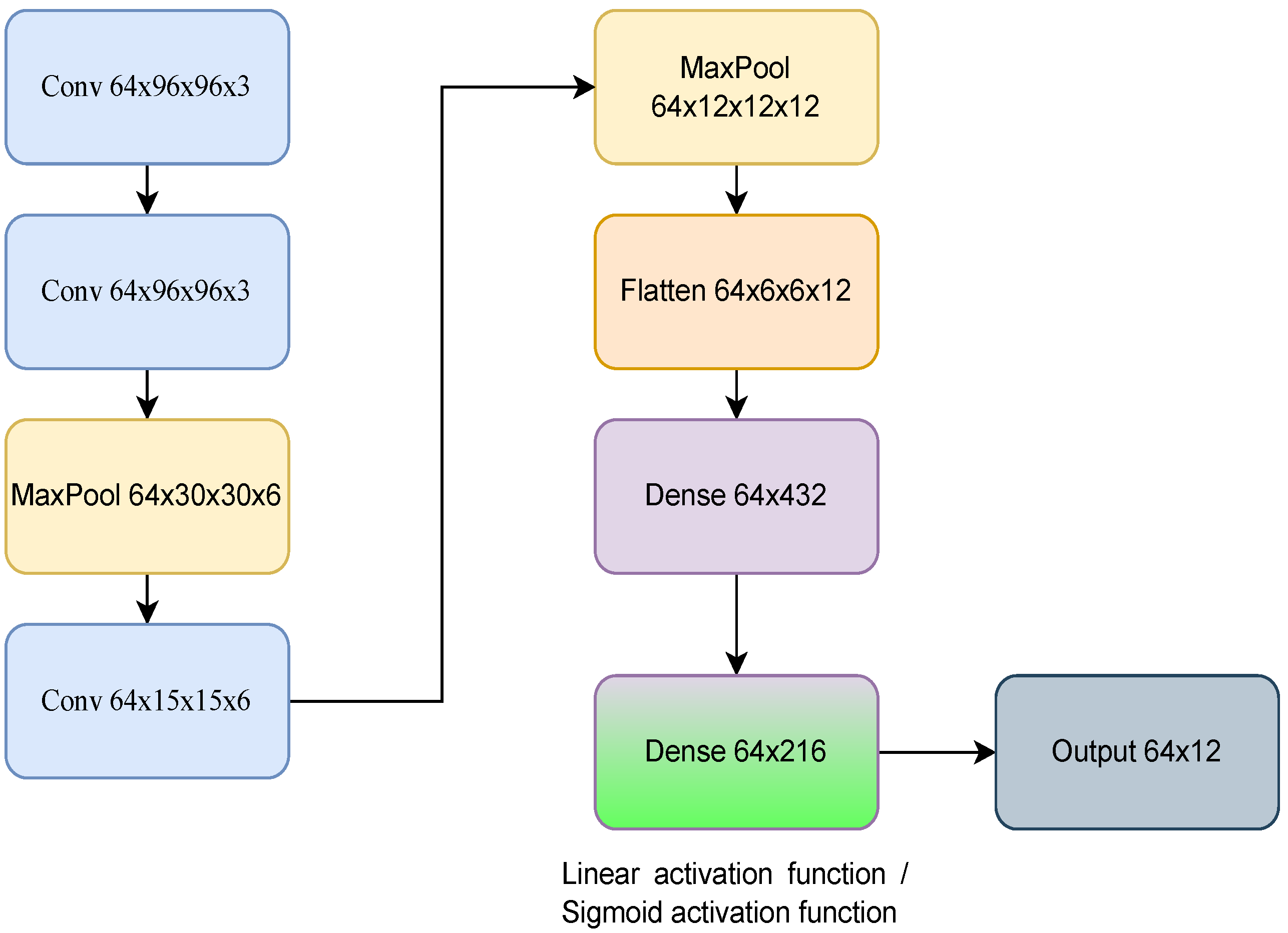
3. Methods and Proposed Architecture

Taking into account the methods based on learning and introspection presented by Cruz et al. [26], an adaptation for a continuous state space was proposed for this study. These methods used the probability of success. This is the probability of reaching the goal in order to provide an explanation with regard to the agent’s decision-making. For instance, an agent executing a task might perform different actions $a_1$ and $a_2$ from a particular state s leading to different probabilities $p_1$ and $p_2$ of completing the task successfully. The probability is linked with the experience the agent has collected during the training and can be estimated using the learning-based and introspection-based methods. Therefore, the learning-based method focused on continuous learning for the probability of success through the ongoing execution of the goal-driven learning algorithm. For the introspection-based method, the Q-values were used in order to infer the probability value of success.

3.1. Learning-Based Method

The learning-based method consisted of using the same idea of goal-driven learning shown in Equation (1), related to temporal-difference algorithms, where $Q(s_t,a_t)$ is the state-action value for a state s and action a at a time t, $\alpha$ is a constant step-size parameter, $r_{t+1}$ is the observed reward, and $\gamma$ is the discount rate parameter. Cruz et al. [26] proposed Equation (2) as a possible solution for calculating the probability of success within discrete environments, where $\mathbb{P}(s_t,a_t)$ is the probability of success for a state s and an action a at a time t, $\alpha$ is a constant step-size parameter and ${\varphi }_{t+1}$ is a binary value representing if the task is completed successfully at a time $t+1$. However, for continuous environments, this equation caused problems because the state space presents infinite possibilities. This made it impossible to use a table of state-action pairs. As a result, we propose working with a parallel artificial neural network and with the same structure used with the algorithm for goal-driven learning that predicts the probability of success.

$$Q(s_t,a_t)\leftarrow Q(s_t,a_t)+\alpha \left[r_{t+1}+\gamma Q(s_{t+1},a_{t+1})-Q(s_t,a_t)\right]$$

(1)

$$\mathbb{P}(s_t,a_t)\leftarrow \mathbb{P}(s_t,a_t)+\alpha [{\varphi }_{t+1}+\mathbb{P}(s_{t+1},a_{t+1})-\mathbb{P}(s_t,a_t)]$$

(2)

The artificial neural network focused on the probability of success used the same structure as that of the DQN algorithm [29], as illustrated in Figure 1. Moreover, the network was updated and used the same loss function as the DQN algorithm. The only difference was that the last dense layer used a sigmoid activation function with the goal of restricting the values in the probability range of 0 and 1. Algorithm 1 shows the implementation of the DQN method with the learning-based approach. In the algorithm, $y_j$ and $y_{pj}$ are the approximate target value for the DQN algorithm and the network used in this method, respectively. $\theta$ are the parameters of the networks. C is the number of steps when the target network is updated with the parameters of the main network, for each case. This number is arbitrarily chosen, for this work has been empirically set to 5. M is the number of episodes. The notation $x_j$ where $x\in \{s,a,r,done\}$ refers to the transition elements within the D memory. The calculation of the probability using this method is illustrated between lines 16 and 18.

3.2. Introspection-Based Method

Cruz et al. [26] proposed Equation (3) to compute the probability of success according to the introspection-based method. This solution consists of estimating the probability using the Q-value through a mathematical transformation, so no additional memory is needed. In the equation, $\sigma$ is a parameter for stochastic transitions (in this case 0). $Q^{\ast }(s,a)$ is the estimated Q-value. $R^T$ is the total reward obtained at the terminal state. ${\left[\dots \right]}_{\widehat{P_S}\ge 0}^{\widehat{P_S}\le 1}$ is the rectification used to restrict the value between $[0,1]$.

For continuous environments, a normalization of the results was proposed instead of limiting it with the equation. The change is illustrated in Equation (4) where $\widehat{p_S}$ relates to the normalization of a probability and $\hat{p}$ computes the probability as shows in Equation (3) without the rectification. Algorithm 2 shows an adaptation of the introspection-based method in addition to the DQN algorithm [29]. In the algorithm, the notation used is as in Algorithm 1. The calculation for the probability of this method was carried out in line 17.

$$\widehat{P_S}\approx {\left[(1-\sigma )·(\frac{1}{2}·log\frac{Q^{\ast }(s,a)}{R^T}+1)\right]}_{\widehat{P_S}\ge 0}^{\widehat{P_S}\le 1}$$

(3)

$$\begin{array}{cc}\hfill \widehat{P_S}& \approx \widehat{p_S}\in \hat{P}\hfill \\ \hfill \widehat{p_S}& =\frac{\hat{p}-min\left(\hat{P}\right)}{max\left(\hat{P}\right)-min\left(\hat{P}\right)}\hfill \\ \hfill \hat{p}& =(1-\sigma )·(\frac{1}{2}·log\frac{Q^{\ast }(s,a)}{R^T}+1)\hfill \end{array}$$

(4)

Algorithm 1 Explainable goal-driven learning approach to calculate the probability of success using the learning-based method.

1: Initialize Q and $\mathbb{P}$ functions   2: Initialize $\hat{Q}$ and $\hat{\mathbb{P}}$ function objectives   3: Initialize memory D with long N   4: for episode 1 to M do   5:     Initialize state queue S with initial state   6:     repeat   7:         $ϵ\leftarrow$ update $ϵ$ with $ϵ$-decay   8:         $s_t\leftarrow$ dequeue current state from S   9:         Select an action $a_t$ according to $s_t$ using policy $ϵ$-greedy 10:         Take action $a_t$, observe reward $r_t$, and next state $s_{t+1}$ 11:         Enqueue next state $s_{t+1}$ into S 12:         Store transition $(s_t,a_t,r_t,s_{t+1},don{e}_t)$ in D 13:         Take a random sample of transitions $(s_j,a_j,r_j,s_{j+1},don{e}_j)$ from D 14:         $y_j=\left\{\begin{array}{cc}{r}_j& \mathrm{if}{s}_{t+1}\mathrm{is}\mathrm{final}\hfill \\ r_j+\gamma {max}_{a^{\prime }}\hat{Q}(s_{j+1},a^{\prime })& \mathrm{otherwise}\hfill \end{array}\right.$ 15:         Update Q with respect to $y_j$ 16:         $y_{pj}=\left\{\begin{array}{cc}{r}_j& \mathrm{if}{s}_{j+1}\mathrm{is}\mathrm{final}\hfill \\ r_j+\gamma {max}_{a^{\prime }}\hat{\mathbb{P}}(s_{t+1},a^{\prime })& \mathrm{otherwise}\hfill \end{array}\right.$ 17:         Update $\mathbb{P}$ related to $y_{pj}$ 18:         Each C steps, ${\theta }_{\hat{Q}}\leftarrow {\theta }_Q$ y ${\theta }_{\hat{\mathbb{P}}}\leftarrow {\theta }_{\mathbb{P}}$ 19:     until $s_t$ is terminal or $r_t$ had been negative 25 times 20: end for 21: Return $Q,\mathbb{P}$

Algorithm 2 Explainable goal-driven reinforcement learning approach for computing the probability of success using the introspection-based method. The algorithm is mainly based on [29] and includes the probabilistic introspection-based method.

1: Initialize function Q   2: Initialize $\hat{Q}$ function objective   3: Initialize memory D with long N   4: for episode 1 to M do   5:     Initialize state queue S with initial state   6:     repeat   7:         $ϵ\leftarrow$ update $ϵ$ with $ϵ$-decay   8:         $s_t\leftarrow$ dequeue current state from S   9:         Select an $a_t$ action according the $s_t$ state using $ϵ$-greedy policy 10:         Take action $a_t$, observe reward $r_t$, and next $s_{t+1}$ state 11:         Enqueue next state $s_{t+1}$ into S 12:         Store the transition $(s_t,a_t,r_t,s_{t+1},don{e}_t)$ in D 13:         Take a random sample of the transitions $(s_j,a_j,r_j,s_{j+1},don{e}_j)$ from D 14:         $y_j=\left\{\begin{array}{cc}{r}_j& \mathrm{if}{s}_{t+1}\mathrm{is}\mathrm{final}\hfill \\ r_j+\gamma {max}_{a^{\prime }}\hat{Q}(s_{j+1},a^{\prime })& \mathrm{otherwise}\hfill \end{array}\right.$ 15:         Update Q related to $y_j$ 16:         Each C steps, ${\theta }_{\hat{Q}}\leftarrow {\theta }_Q$ 17:         $\widehat{P_S}\approx \widehat{p_S}\in \hat{P}$ 18:     until $s_t$ is terminal or $r_t$ had been negative 25 times 19: end for 20: Return $Q,\widehat{P_S}$

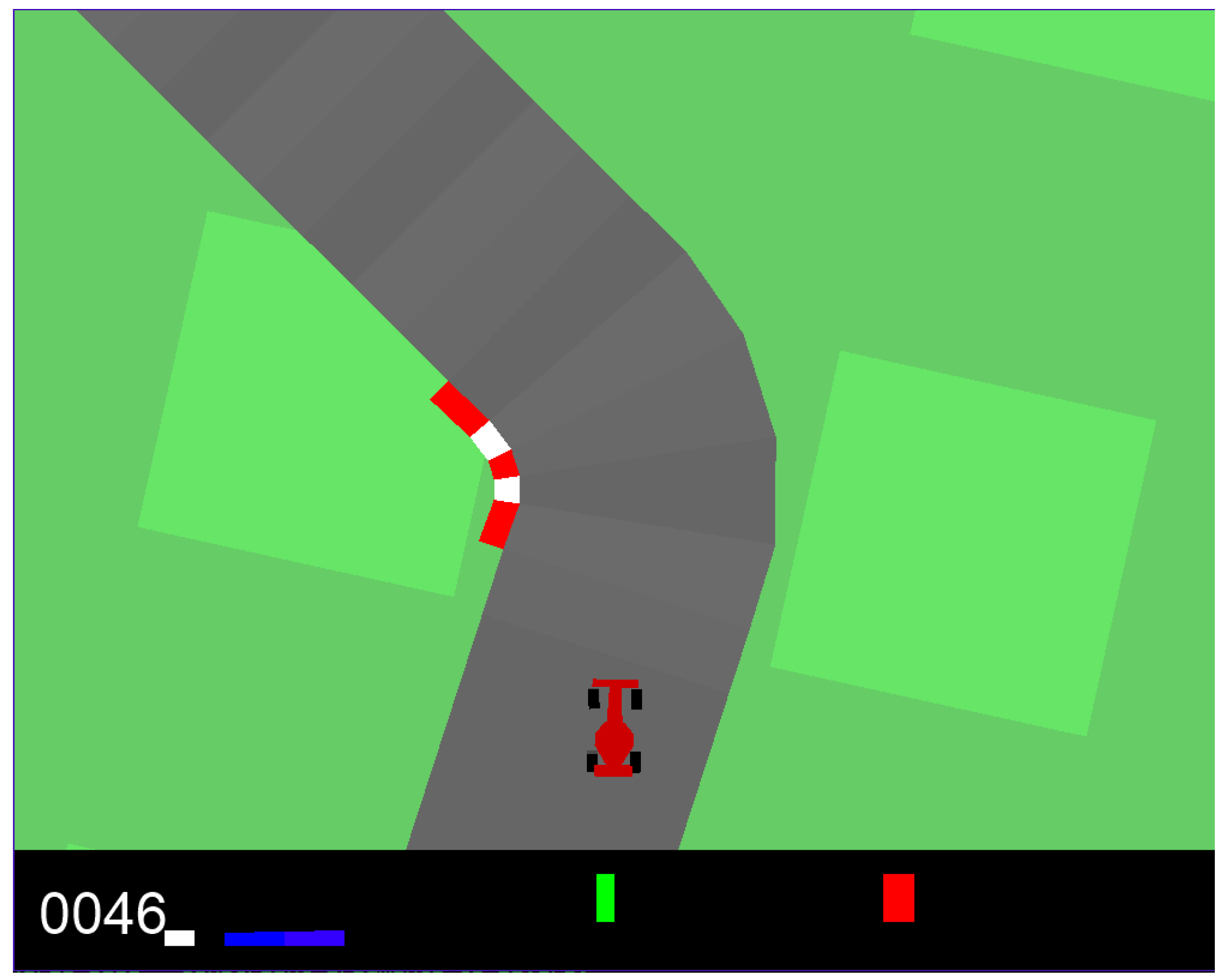
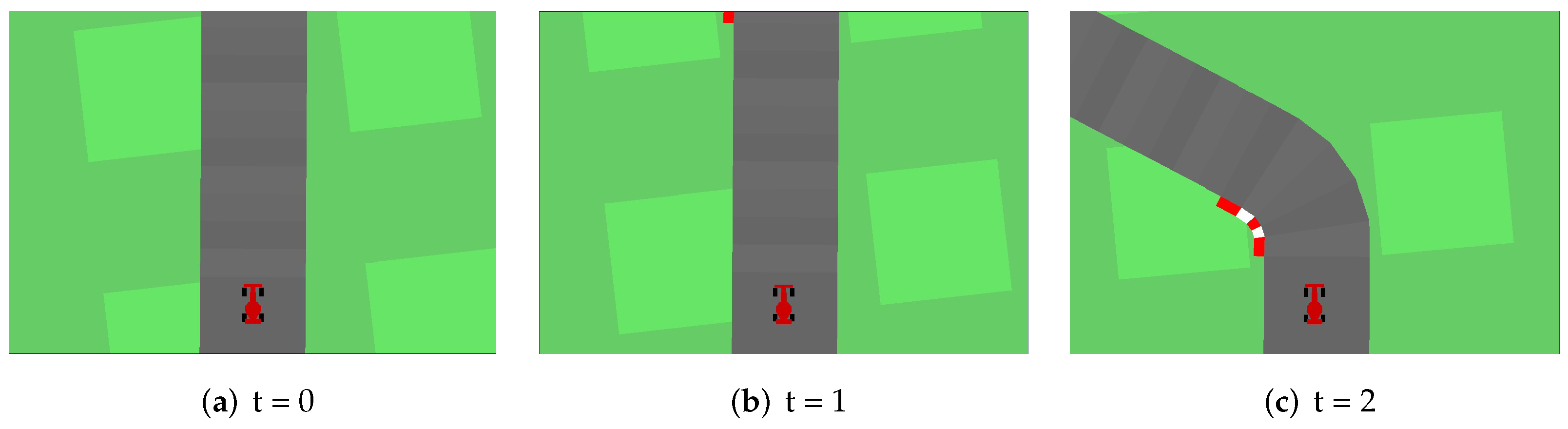
4. Experimental Scenario

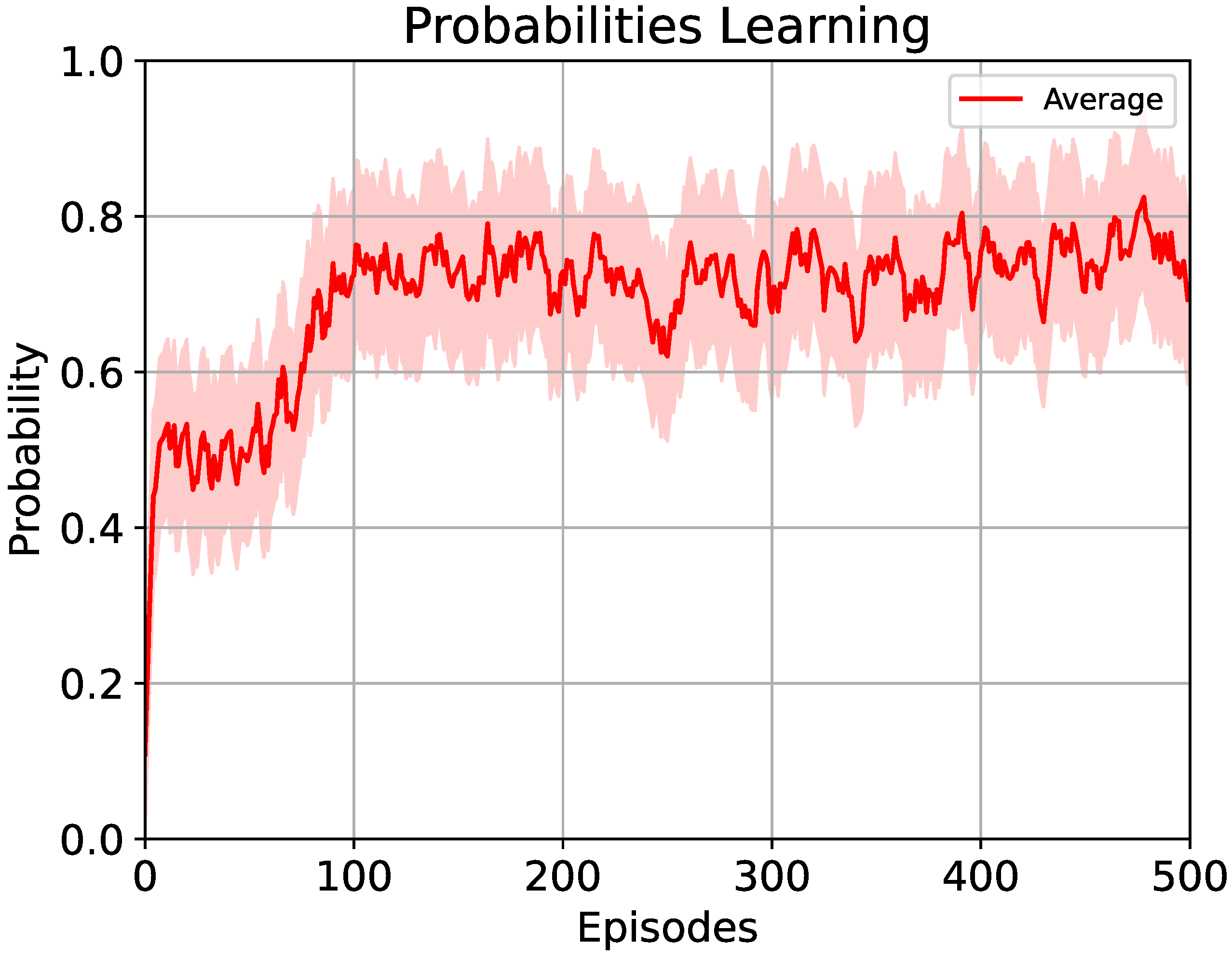
The experimental scenario was implemented using the Open AI Gym library [30]. It facilitated the development of goal-driven learning algorithms. Specifically, the environment that situated the car racing game (see Figure 2) was selected since it is a continuous environment. Deep Q-Network (DQN) was used for learning, and Keras was used to create the neural network. Furthermore, the decay $ϵ$-greedy method was chosen for action selection.

The environment consisted of a race track where a car was controlled by an autonomous agent. The objective was to take a lap around the track. The images of the environment were preprocessed by converting them to a gray scale. Following, the state was represented by three consecutive images of the game (Figure 3). Each image consisted of a matrix of $96\times 96$ pixels, so the state remained represented by a matrix of $96\times 96\times 3$. The initial state of the environment related to a random generation of the race track where the car could start at any point on the track. Actions were carried out with a combination of movements with the steering wheel (−1, 0, 1), acceleration (0 or 1), and braking (0 or 1), resulting in a total of $3\times 2\times 2=12$ possible actions. Therefore, in this work, we have used a continuous state space and a discrete action space.

The reward within the environment is displayed in Equation (5) where $N_B$ represents the number of boxes on the track and f the quantity of frames used. It is important to take into account the implementation included a 50% bonus if the agent used the accelerator without braking.

$$r\left(f\right)=\left\{\begin{array}{cc}1.5\ast (\frac{1000}{N_B}-0.1\ast f)\hfill & \mathrm{Acceleration}\mathrm{without}\mathrm{braking}\hfill \\ \frac{1000}{N_B}-0.1\ast f\hfill & \mathrm{The}\mathrm{opposite}\mathrm{case}\hfill \end{array}\right.$$

(5)

5. Results

Two experiments were conducted for this research. The first experiment focused on adapting the methods for calculating the probability of success for both methods. One agent was trained with the DQN algorithm five times and the learning-based and introspection-based methods were used to compute the probability of success within the experimental scenario. In the second experiment, the use of resources was analyzed. In this regard, one agent was trained using each of the proposed probabilistic methods for three runs. The parameters used during this process included: initial $ϵ=1.0$, $ϵ$-decay ${ϵ}_{decay}=0.9999$, and learning rate $\alpha =0.001$.

5.1. Adaptation of the Explainability Methods

Figure 4 displays the results for the average Q-values for the twelve possible actions of the agent through each of the five training experiments. Furthermore, Figure 5 illustrates the total collected reward for five runs. Both graphs show the values for each agent throughout 500 episodes using the DQN algorithm. Moreover, both graphs are smoothed with the moving averages method with discrete linear convolutions with a set of 30 data. These values are depicted as reference points for analyzing the results for the probability of success.

5.1.1. Learning-Based Method

Results were obtained as shown in Figure 6. These consist of the averages of the probabilities of success for each episode during five training processes. For each agent, an average of the probabilities for all of the actions was computed according to a dedicated artificial neural network. In the first 75 episodes, the average of the probability remained relatively constant $\mathbb{P}\approx 0.5$. Around episode 75, the agents showed an improvement in probability, but stopped at approximately episode 100 with a value of $\mathbb{P}\approx 0.75$. Later, the probability of success fluctuated in the remainder of the training staying close to the value mentioned. This can be interpreted that around episode 500, the agent had a 75% probability of completing the task. Although for the explainability method, the best action to perform is not much relevant, this is decided using the DQN algorithm. Therefore, the results obtained show the probability of success assuming the optimal action for each possible state. For example, if a car racing player would like to ask the agent why on the first curve of the track it turned left instead of right, with the probability of success, the agent might respond: “I have 75% probability of finishing the track if I select this action.” However, if it were to respond with the Q-value, “I have a Q-value $\approx 80$.” For the player of the game, this would make no sense.

Even when the adaptation proposed was related directly to the Q-values, a stepped behavior was observed for the case of probability. However, in the case of Q-values, these are similar to an increasing linear behavior.

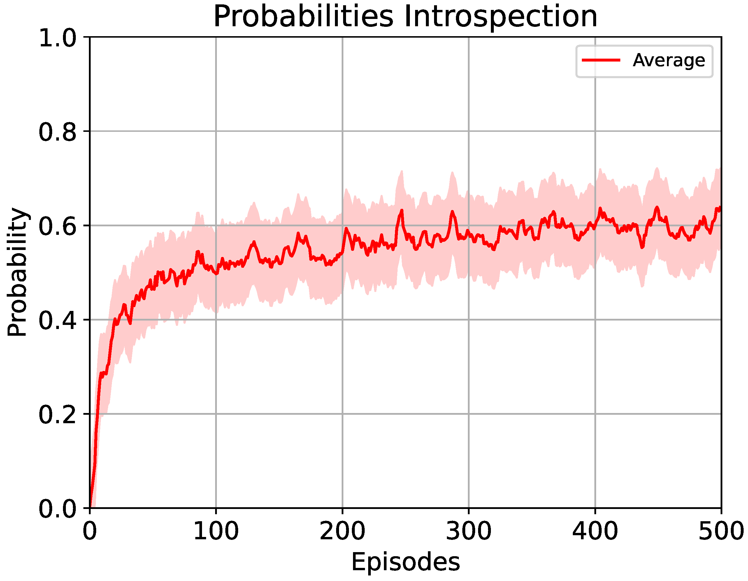
5.1.2. Introspection-Based Method

The results for the introspection-based method are displayed in Figure 7. These consist of the average of the probabilities of success for five training processes during 500 episodes, similar to the previous method. The average of the probabilities was obtained for each agent for the twelve actions calculated with those of Equation (4). An increase in the average of the probability of success in the first 75 episodes reached a value of ${\hat{P}}_S=0.5$. Later, it continued to increase subtly, ending with a probability of success with a value of ${\hat{P}}_S=0.62$. Thus, this could be interpreted that at episode 500, the agent had a 62% probability of completing the task. A logarithmic behavior was observed supported by the function presented in Equation (3). Similarly, the agent could explain to the user that it had, for example, a 62% probability of finishing the track if it continued going straight in the last section instead of turning right. What is important in this sense is that the user understands the decision making.

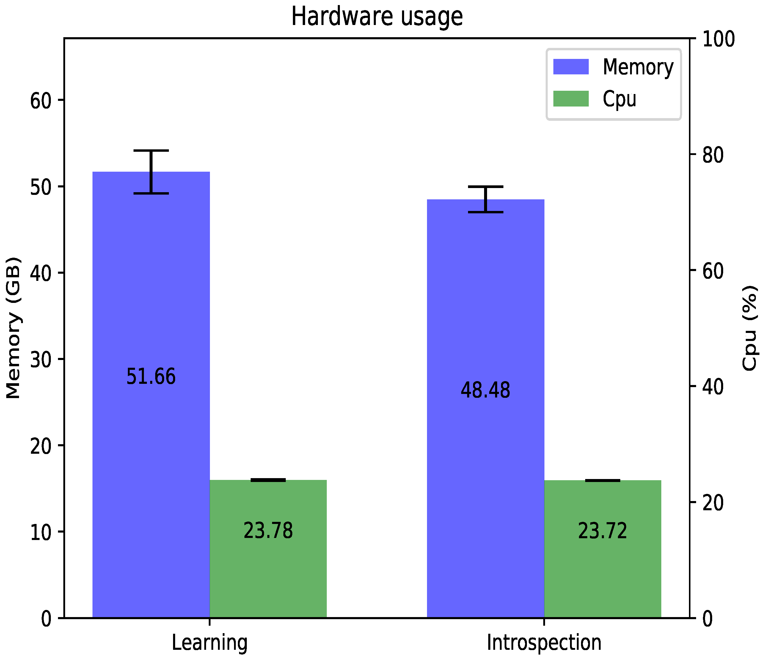
5.2. Use of Resources

An additional experiment was carried out to measure the use of resources of the methods adapted to the continuous environments. This experiment was performed with an agent for each method, each agent was trained three times during 200 episodes. The goal of the experiment was to measure the RAM memory and the use of the processor (CPU). For this, the Python psutil library was consulted.

In the training environment, the agent processed and stored images. Therefore, the amount of memory used for this process was significant. As a result, both experiments were carried out in periods of 40 episodes until the number of episodes completed corresponded to each experiment. Based on these conditions for each agent, the memory used and the use of the CPU were recorded for each of these periods. In the case of memory, all of the periods recorded were added together, and in the case of the CPU, periods were averaged. The computer used for these experiments had a Windows Pro operating system, an Intel^® Core^TM i5-8500 @3 GHz processor, and a two memory RAM HyperX^® FURY 8GB DDR4 2666 MHz.

The results are illustrated in Figure 8, where each method has similar values for use of the CPU. With regard to the memory used for the methods, a slight difference occurred in favor of the introspection-based method with an average of 93% memory occupied and 98% of memory occupied for the learning-based method with a lower standard deviation that indicated greater stability using this resource.

5.3. Discussion

In the learning-based method, changes were made in the tests for adapting to a continuous state space. In principle, the neural network used for probability of success was tried to provide the objective for Equation (2). Thus, the fixed discount factor of 1 was used as it appeared in the equation. In addition, the reward was not used to update the values. Instead, the binary variable corresponded to 0 if the task had not been completed and to a 1 if the task had been completed, designated as $\varphi$.

After a few of the experiments, some inconsistencies were observed in the results, such as the structure of the neural network. It had layers of functions for activating the rectified linear unit (RELU). The probability was not limited between 0 and 1. As a result, the activation of the last layer was changed to a sigmoid with the goal of obtaining values in the interval $[0,1]$. This change did not have good results. Throughout the episodes, the probability remained static with a value of $0.6$.

Finally, the adaptation method, proposed in Section 3, similar to the DQN algorithm, occupied a network to learn the probability of success, maintaining the discount factor and reward for calculating the probability of success. The difference in the last layer had a sigmoid as activation function.

With regard to the introspection-based method, similarly, an attempt was made to implement it as shown in Equation (3). However, the results suggested that the upper limit obstructed part of the results. Then, the normalization of the data was proposed so that it would remain in interval $[0,1]$. Therefore, in Equation (3), the notation ${\left[\dots \right]}_{\widehat{P_S}\ge 0}^{\widehat{P_S}\le 1}$, which represented the rectification, was replaced with the normalization function presented in Equation (4) where $\widehat{P_S}$ corresponded to a set of probability success data calculated with the transformation value of Q and $R^T$.

The learning-based method underwent the most changes due to the replacement of the probability table (discrete) with an artificial neural network (continuous) for learning the probabilities. In addition, the way of calculating the probability was proposed similar to that of the DQN algorithm. However, for the introspection method, the proposal was made to change the rectification of the probability with normalization with the values obtained.

On the other hand, in the context of the second experiment, the a priori estimated that in the learning-based method, resources would be more expensive. However, based on the proposal for this method, RAM memory use remained close to that of the introspection-based method. Since the proposed algorithm in discrete settings occupied a table with the same dimensions as the table for the Q-values, in adapting the learning method, it was replaced by an artificial neural network that substituted memory use for processing use. Even though it was an improvement for memory use, it continued to need more memory than did the introspection-based method.

Given the obtained results including the estimated probability of success using the learning-based and the introspection-based methods as well as the use of resources, we hypothesize that the learning-based method would be preferred in simpler scenarios in which to run a parallel neural network training is not expensive as this gives a better estimation of the probability (as in the car racing game scenario). Contrarily, in more complex scenarios or when the computational resources are limited to run an additional neural network, the introspection-based method should be considered, as the estimation of the probability can be computed directly from the Q-values and, therefore, no additional memory is needed.

6. Conclusions

In this present study, the explainability methods were tested and adapted for a continuous environment: one based on learning and the other based on introspection. Therefore, it was necessary to adapt the methods so that it would be possible to carry them out within a continuous environment. The advantage of estimating the probability of success by the learning-based and introspection-based methods in comparison to a memory-based method [25] is that the latter implies saving the agent’s transitions into a memory to compute the probability of success later on. Although that method is an effective and reliable manner to compute the probability of success, it is very inefficient as the number of transitions grows. This is especially relevant in continuous or real-world scenarios. Therefore, computing an estimation of the probability of success using either the learning-based or introspection-based methods would allow the proposed explainability framework to scale to more complex scenarios.

Two experiments were conducted focused on the explainability methods and their use of resources. In the first case, the learning-based method was associated with the idea of the probability of success learned through the training, but with a change in the way it was performed, obtaining an average of $\mathbb{P}=0.75$ at the end of training. On the other hand, the basis of the introspection-based method was to maintain and change the correction of the normalization of the data resulting in an average of $\widehat{P_S}=0.62$. From these advances, human–agent interaction methods can be improved to become closer to reality. In essence, this could create the trust necessary so that they could function fully. In the second experiment, with respect to the use of resources, the use of the CPU did not present any significant differences between the two methods. However, the learning-based method used more memory with an average of $51.66$ GB for 200 episodes in comparison to $48.48$ GB for the introspection-based method, due to the operation of the second artificial neural network used with the learning-based method.

In this work, we have used the well-known DQN algorithm, however, more efficient RL algorithms should be considered in the future. Although agent performance was not the aim of this work, we hypothesize that a better base RL method may also lead to better explanations. Some algorithms interesting to further explore are Soft Actor-Critic [31] or Rainbow [32] that use previous deep RL methods such as double Q-learning, prioritized replay, dueling networks, multi-step learning, distributional RL, and noisy nets including recommended parameters. Moreover, as we have only used the car racing game scenario with a continuous state space, additional experiments are needed for a comprehensive evaluation in continuous environments, for instance, including those evaluated by Mnih et al. [33] or with continuous action spaces [34]. Nevertheless, our work presents a baseline to further evaluate goal-driven explainability reinforcement learning methods in continuous scenarios.

References

1. Singhal, A.; Sinha, P.; Pant, R. Use of deep learning in modern recommendation system: A summary of recent works. arXiv 2017, arXiv:1712.07525. [Google Scholar] [CrossRef]
2. Bhuiyan, H.; Ashiquzzaman, A.; Juthi, T.I.; Biswas, S.; Ara, J. A survey of existing e-mail spam filtering methods considering machine learning techniques. Glob. J. Comput. Sci. Technol. 2018, 18, 21–29. [Google Scholar]
3. Guo, G.; Zhang, N. A survey on deep learning based face recognition. Comput. Vis. Image Underst. 2019, 189, 102805. [Google Scholar] [CrossRef]
4. Alanazi, H.O.; Abdullah, A.H.; Qureshi, K.N. A critical review for developing accurate and dynamic predictive models using machine learning methods in medicine and health care. J. Med. Syst. 2017, 41, 69. [Google Scholar] [CrossRef]
5. Aradi, S. Survey of deep reinforcement learning for motion planning of autonomous vehicles. IEEE Trans. Intell. Transp. Syst. 2020, 23, 740–759. [Google Scholar] [CrossRef]
6. Das, A.; Rad, P. Opportunities and challenges in explainable artificial intelligence (xai): A survey. arXiv 2020, arXiv:2006.11371. [Google Scholar]
7. Dazeley, R.; Vamplew, P.; Foale, C.; Young, C.; Aryal, S.; Cruz, F. Levels of explainable artificial intelligence for human-aligned conversational explanations. Artif. Intell. 2021, 299, 103525. [Google Scholar] [CrossRef]
8. Lim, B.Y.; Dey, A.K.; Avrahami, D. Why and why not explanations improve the intelligibility of context-aware intelligent systems. In Proceedings of the SIGCHI Conference on Human Factors in Computing Systems, Boston, MA, USA, 4–9 April 2009; pp. 2119–2128. [Google Scholar]
9. Cruz, F.; Acuña, G.; Cubillos, F.; Moreno, V.; Bassi, D. Indirect training of grey-box models: Application to a bioprocess. In International Symposium on Neural Networks; Springer: Berlin/Heidelberg, Germany, 2007; pp. 391–397. [Google Scholar]
10. Naranjo, F.C.; Leiva, G.A. Indirect training with error backpropagation in Gray-Box Neural Model: Application to a chemical process. In Proceedings of the 2010 XXIX International Conference of the Chilean Computer Science Society, Antofagasta, Chile, 15–19 November 2010; pp. 265–269. [Google Scholar]
11. Ayala, A.; Cruz, F.; Fernandes, B.; Dazeley, R. Explainable Deep Reinforcement Learning Using Introspection in a Non-episodic Task. arXiv 2021, arXiv:2108.08911. [Google Scholar]
12. Barros, P.; Tanevska, A.; Cruz, F.; Sciutti, A. Moody Learners-Explaining Competitive Behaviour of Reinforcement Learning Agents. In Proceedings of the 2020 Joint IEEE 10th International Conference on Development and Learning and Epigenetic Robotics (ICDL-EpiRob), Valparaiso, Chile, 7–11 September 2020; pp. 1–8. [Google Scholar]
13. Dazeley, R.; Vamplew, P.; Cruz, F. Explainable reinforcement learning for Broad-XAI: A conceptual framework and survey. arXiv 2021, arXiv:2108.09003. [Google Scholar]
14. Gunning, D.; Aha, D. DARPA’s Explainable Artificial Intelligence (XAI) Program. AI Mag. 2019, 40, 44–58. [Google Scholar] [CrossRef]
15. Sado, F.; Loo, C.K.; Liew, W.S.; Kerzel, M.; Wermter, S. Explainable Goal-Driven Agents and Robots—A Comprehensive Review. arXiv 2020, arXiv:2004.09705. [Google Scholar]
16. Sutton, R.S.; Barto, A.G. Reinforcement Learning: An Introduction; MIT Press: Cambridge, MA, USA, 2018. [Google Scholar]
17. Goodrich, M.A.; Schultz, A.C. Human-Robot Interaction: A Survey, Foundations and Trends in Human-Computer Interaction. 2007. Available online: https://www.researchgate.net/publication/220613473_Human-Robot_Interaction_A_Survey (accessed on 30 January 2022).
18. Millán, C.; Fernandes, B.J.; Cruz, F. Human feedback in Continuous Actor-Critic Reinforcement Learning. In Proceedings of the European Symposium on Artificial Neural Networks, Computational Intelligence and Machine Learning ESANN, Bruges, Belgium, 24–26 April 2019; pp. 661–666. [Google Scholar]
19. Adadi, A.; Berrada, M. Peeking inside the black-box: A survey on explainable artificial intelligence (XAI). IEEE Access 2018, 6, 52138–52160. [Google Scholar] [CrossRef]
20. Lamy, J.B.; Sekar, B.; Guezennec, G.; Bouaud, J.; Séroussi, B. Explainable artificial intelligence for breast cancer: A visual case-based reasoning approach. Artif. Intell. Med. 2019, 94, 42–53. [Google Scholar] [CrossRef] [PubMed]
21. Wang, X.; Chen, Y.; Yang, J.; Wu, L.; Wu, Z.; Xie, X. A reinforcement learning framework for explainable recommendation. In Proceedings of the 2018 IEEE International Conference on Data Mining (ICDM), Singapore, 17–20 November 2018; pp. 587–596. [Google Scholar]
22. He, L.; Aouf, N.; Song, B. Explainable Deep Reinforcement Learning for UAV autonomous path planning. Aerosp. Sci. Technol. 2021, 118, 107052. [Google Scholar] [CrossRef]
23. Madumal, P.; Miller, T.; Sonenberg, L.; Vetere, F. Explainable reinforcement learning through a causal lens. In Proceedings of the AAAI Conference on Artificial Intelligence, New York, NY, USA, 7–12 February 2020; Volume 34, pp. 2493–2500. [Google Scholar]
24. Sequeira, P.; Gervasio, M. Interestingness elements for explainable reinforcement learning: Understanding agents’ capabilities and limitations. Artif. Intell. 2020, 288, 103367. [Google Scholar] [CrossRef]
25. Cruz, F.; Dazeley, R.; Vamplew, P. Memory-based explainable reinforcement learning. In Proceedings of the Australasian Joint Conference on Artificial Intelligence, Adelaide, SA, Australia, 2–5 December 2019; Springer: Berlin/Heidelberg, Germany, 2019; pp. 66–77. [Google Scholar]
26. Cruz, F.; Dazeley, R.; Vamplew, P. Explainable robotic systems: Understanding goal-driven actions in a reinforcement learning scenario. Neural Comput. Appl. 2021. [Google Scholar] [CrossRef]
27. Milani, S.; Topin, N.; Veloso, M.; Fang, F. A Survey of Explainable Reinforcement Learning. arXiv 2022, arXiv:2202.08434. [Google Scholar]
28. Heuillet, A.; Couthouis, F.; Díaz-Rodríguez, N. Explainability in deep reinforcement learning. Knowl.-Based Syst. 2021, 214, 106685. [Google Scholar] [CrossRef]
29. Mnih, V.; Kavukcuoglu, K.; Silver, D.; Rusu, A.; Veness, J.; Bellemare, M.G.; Graves, A.; Riedmiller, M.; Fidjeland, A.K.; Ostrovski, G.; et al. Human-level control through deep reinforcement learning. Nature 2015, 518, 529–533. [Google Scholar] [CrossRef]
30. Brockman, G.; Cheung, V.; Pettersson, L.; Schneider, J.; Schulman, J.; Tang, J.; Zaremba, W. Openai gym. arXiv 2016, arXiv:1606.01540. [Google Scholar]
31. Haarnoja, T.; Zhou, A.; Abbeel, P.; Levine, S. Soft actor-critic: Off-policy maximum entropy deep reinforcement learning with a stochastic actor. In Proceedings of the International Conference on Machine Learning, Stockholm, Sweden, 10–15 July 2018; pp. 1861–1870. [Google Scholar]
32. Hessel, M.; Modayil, J.; Van Hasselt, H.; Schaul, T.; Ostrovski, G.; Dabney, W.; Horgan, D.; Piot, B.; Azar, M.; Silver, D. Rainbow: Combining improvements in deep reinforcement learning. In Proceedings of the Thirty-Second AAAI Conference on Artificial Intelligence, New Orleans, LA, USA, 2–7 February 2018. [Google Scholar]
33. Mnih, V.; Kavukcuoglu, K.; Silver, D.; Graves, A.; Antonoglou, I.; Wierstra, D.; Riedmiller, M. Playing atari with deep reinforcement learning. arXiv 2013, arXiv:1312.5602. [Google Scholar]
34. Gupta, J.K.; Egorov, M.; Kochenderfer, M. Cooperative multi-agent control using deep reinforcement learning. In Proceedings of the International Conference on Autonomous Agents and Multiagent Systems, São Paulo, Brazil, 8–12 May 2017; Springer: Berlin/Heidelberg, Germany, 2017; pp. 66–83. [Google Scholar]
Figure 1. Diagram of the neural network used to calculate the Q-values using the DQN algorithm and the probability of success using the learning-based method. When computing the probability of success, the neural architecture used a sigmoid activation function in the last dense layer in order to restrict the output values between 0 and 1. Three consecutive 96 × 96 gray images of the car racing game are used as inputs.
Algorithms 15 00091 g001
Figure 2. Experimental scenario. In the image from left to right, colors depict velocity (white), the four ABS sensors (blue and purple), the position of the steering wheel (green), and the gyroscope (red).
Algorithms 15 00091 g002
Figure 3. The input is represented by three consecutive images of 96 × 96 (matrix of 96 × 96 × 3 ) from the car racing game. The images in the figure are examples since they were previously processed in a gray scale.
Algorithms 15 00091 g003
Figure 4. Averaged Q-values for five runs using the DQN algorithm during 500 episodes. The Q-values are averaged for each episode considering twelve possible actions. The results are smoothed in a window of 30 data using a linear convolution.
Algorithms 15 00091 g004
Figure 5. Total reward for five runs using the DQN algorithm during 500 episodes. In the figure, the collected rewards are smoothed in a window of 30 data using a linear convolution.
Algorithms 15 00091 g005
Figure 6. Average value of the probability of success for five runs of the agent’s training during 500 episodes using the learning-based method proposed in Algorithm 1. The probability value is smoothed and the shaded area refers to the standard deviation.
Algorithms 15 00091 g006
Figure 7. Average values for the probability of success for five runs of the agent’s training during 500 episodes using the introspection-based method proposed in Algorithm 2. The probability value is smoothed and the shaded area represents the standard deviation.
Algorithms 15 00091 g007
Figure 8. Values for use of resources considering RAM memory and percentage of processor use (CPU). Average value and standard deviation are computed for three training processes during 200 episodes for each method. The y axis on the left relates to the gigabyte scale, and the percentage is on the right. A lower standard deviation is shown for the introspection method for memory use. This indicates greater stability using this resource. For the case of the CPU, both methods maintained a not null standard deviation close to 0.
Algorithms 15 00091 g008
Publisher’s Note: MDPI stays neutral with regard to jurisdictional claims in published maps and institutional affiliations.