Calculation of Overhead Insulated Cable Ampacity Considering Compacted Conductor Structure

Abstract

The radial heat transfer mechanism of compacted conductors in overhead insulated cables is unclear, and the insulation layer complicates the thermal boundary conditions, limiting the direct applicability of existing ampacity calculation methods. Based on the Morgan model framework, this paper proposes an ampacity calculation method that accounts for the “plastic-then-elastic” deformation characteristics of compacted conductors. Material plastic flow and elastic deformation of the substrate are incorporated to refine the formulations for interlayer thermal contact conductance and thin-layer air gap thickness, while the equivalent distance of air voids is corrected using the fill factor. An iterative convergence procedure for the insulation outer surface temperature is established to accurately evaluate conductor Joule losses. Validated by wind tunnel tests on JKLGYJ 240/30 cables, the proposed method yields a radial temperature difference of 2.41 °C, closely matching the measured 2.6 °C, with an error of 7.4% compared to 13.5% for the conventional Morgan model. Parametric analysis reveals that equivalent radial thermal conductivity is independent of external environmental factors. Conductor stress has a negligible effect on the ampacity (variation < 0.1%). Under low wind speeds (0–5 m/s), the ampacity increases substantially with wind speed.

1. Introduction

Overhead insulated cable is a transmission line composed of a compacted conductor extruded with insulating material [1]. It effectively shortens the phase-to-phase safety distance and reduces the risk of short circuits caused by tree contact [2], making it widely used in densely populated areas, forests, and grasslands. According to statistics [3], the insulation rate of overhead lines in China’s rural power grid increased from 13.69% in 2015 to 50.12% in 2024. With the continuous increase in insulation rates, the ampacity calculation and condition assessment methods for overhead insulated cables urgently require improvement.

Ampacity is a key parameter that characterizes the transmission capacity of a line. Its accurate calculation is fundamental for line condition assessment [4], dynamic capacity expansion [5], and economic operation [6]. For bare overhead conductors, CIGRE TB 207 [7] and TB 601 [8] provide ampacity assessment methods for different current density and temperature ranges. IEEE Std 738 [9] also establishes a similar current–temperature relationship model. Comparative analyses of these standards have been conducted in the literature, with studies indicating that the CIGRE method offers higher accuracy in regions characterized by complex meteorological conditions [10]. In recent years, due to the widespread use of technologies like dynamic rating [11], improving the accuracy of ampacity assessment for overhead insulated cables has become a research hotspot.

Radial temperature distribution is one of the key factors affecting the accuracy of ampacity assessment. Morgan [12] proposed an early method for calculating the radial temperature difference in overhead conductors, laying the theoretical foundation for interlayer contact thermal resistance analysis. Dong et al. [13] verified the applicability of the Morgan model for stranded conductors through wind tunnel tests. Minambres et al. [14] developed a finite element model to analyze the radial temperature distribution in ACSR conductors, considering the heat transfer between layers and with the external environment under both steady-state and transient conditions. Wang et al. [15] further established a three-dimensional finite element model for ACSR conductors that accounts for the helical structure of multilayer strands, and their experimental validation demonstrated that the radial temperature difference can reach up to 8 °C under forced convection conditions. Yu et al. [16] investigated the coupled relationship between AC resistance and temperature distribution in ACSR conductors through finite element-assisted analysis, providing insights into the electro-thermal coupling mechanisms that govern radial heat transfer. The above studies have laid an important foundation for understanding the thermal behavior of overhead conductors.

However, the aforementioned studies all focus on bare overhead conductors. Unlike bare conductors, the conductors of overhead insulated cables generally adopt a compacted structure and are covered with insulating material. Therefore, the ampacity calculation for overhead insulated cables faces two major difficulties:

Firstly, quantifying radial heat transfer in compacted conductors is challenging. The conductors of overhead insulated cables generally adopt a compacted structure to reduce the outer diameter and prevent insulation from sinking in. IEC 60287 [17], when calculating the ampacity of power cables that also feature compacted conductors, does not discuss the radial temperature distribution within the conductor. Finite element methods often neglect inter-wire thermal contact resistance when calculating the conductor’s temperature distribution. Although the Morgan model introduces thermal contact resistance between stranded wires, it is based on the purely geometric and plastic deformation assumptions for non-compacted stranded conductors and cannot accurately describe the influence of the compacted conductor’s structural characteristics on the heat transfer process. Currently, systematic research on the contact heat transfer behavior of compacted conductors and its impact on the operating state is lacking.

Secondly, the thermal boundary conditions become more complex. When assessing the ampacity for bare overhead conductors, the conductor surface temperature is typically taken as the long-term permissible operating temperature, allowing direct calculation of heat exchange with the external environment. However, overhead insulated cables are wrapped with an insulating layer, and the outer surface temperature of the insulation cannot be directly specified, rendering the boundary conditions of the heat balance equation difficult to determine.

Addressing these challenges, this paper proposes an improved ampacity calculation method for overhead insulated cables with compacted conductors within the Morgan model framework. The main contributions are fourfold: (i) a radial heat transfer model for compacted conductors is established by incorporating the influence of material plastic flow on interlayer asperity contact and elastic deformation of the substrate, deriving the thin-layer air gap thickness from the contact area ratio, and correcting the equivalent distance of air voids based on the fill factor; (ii) an iterative convergence procedure for the insulation outer surface temperature is developed to enable the coupled solution of conductor Joule losses and temperature distribution; (iii) the proposed method is experimentally validated through wind tunnel tests on JKLGYJ 240/30 cables, demonstrating significant improvement in accuracy compared to the conventional Morgan model; and (iv) parametric analysis is conducted to quantify the effects of ambient temperature, conductor stress, and wind speed on the ampacity of overhead insulated cables, revealing the distinct influence patterns of these factors.

2. Construction of Current–Temperature Relationship for Overhead Insulated Cables

2.1. Thermal Circuit Diagram

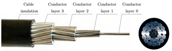
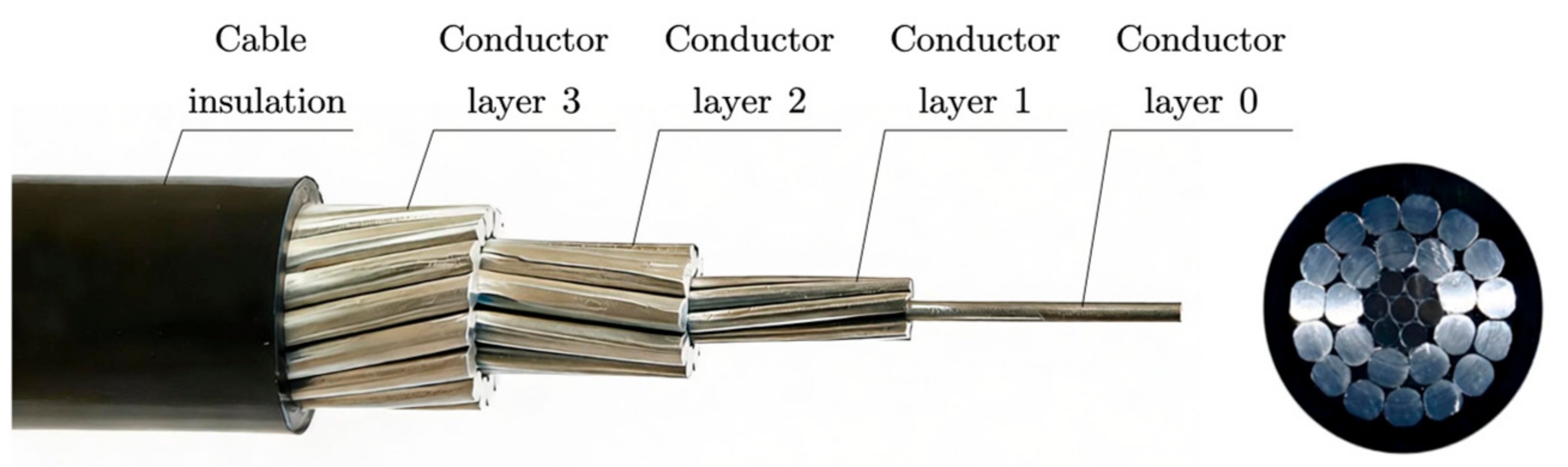
The structure of an overhead insulated cable mainly consists of a conductor and an insulation layer. The conductor, typically made of aluminum core, aluminum alloy core, or steel-reinforced aluminum core, is responsible for current transmission; the insulation layer is generally made of polymer materials such as cross-linked polyethylene, functioning to isolate high-voltage and limit leakage current. To improve the uniformity of the electric field distribution, a semi-conducting shield layer can be arranged between the conductor and the insulation layer. As shown in Figure 1, the structure of the JKLGYJ 240/30–10 kV overhead cable is as follows: the central layer (designated as layer 0) and the first layer are the steel core, while the second and third layers are the aluminum core; the insulation layer is cross-linked polyethylene with a thickness of 3.4 mm; between the conductor and the insulation layer, there is a semi-conducting shield layer with a thickness of 0.6 mm.

Figure 1. Structural diagram of overhead insulated cable.

For overhead insulated cables, the current–temperature relationship adheres to the principle of heat conservation. Under steady-state operation, it satisfies

$$P_{\mathrm{J}}+P_{\mathrm{M}}+P_{\mathrm{S}}+P_{\mathrm{i}}+P_{\mathrm{d}}=P_{\mathrm{c}}+P_{\mathrm{r}}+P_{\mathrm{w}}$$

(1)

where $P_{\mathrm{J}}$ is Joule losses; $P_{\mathrm{M}}$ is magnetic losses in the steel core; $P_{\mathrm{S}}$ is the heat absorbed from solar radiation; $P_{\mathrm{i}}$ is corona loss; $P_{\mathrm{d}}$ is dielectric losses; $P_{\mathrm{c}}$ is the convective heat dissipation; $P_{\mathrm{r}}$ is the radiative heat dissipation; and $P_{\mathrm{W}}$ is the heat dissipation due to evaporation of water droplets attached to the outer surface of the cable.

Overhead insulated cables are mainly used in distribution lines with rated voltages up to 20 kV. The electric field on the insulation outer surface is much lower than the corona inception field strength, so corona losses are neglected ($P_{\mathrm{i}}=0$). The insulation outer surface is hydrophobic, so the evaporative cooling effect is also neglected ($P_{\mathrm{W}}=0$).

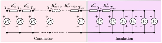
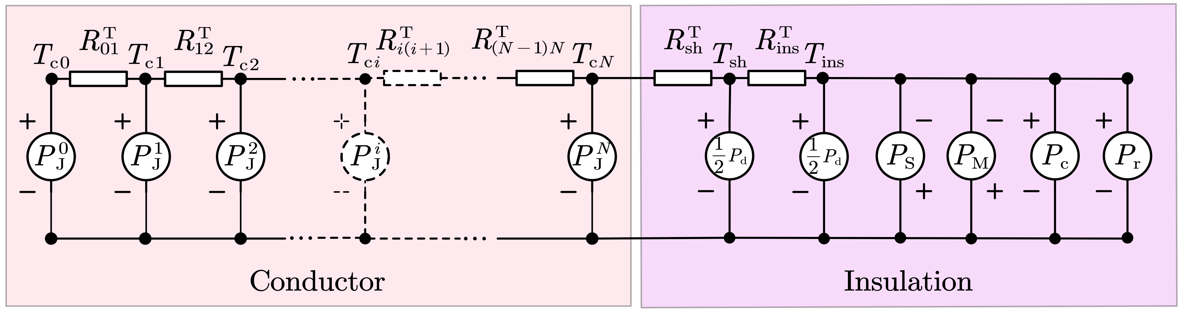
To accurately describe the radial temperature distribution within the compacted conductor structure, a heat transfer model for the layered interfaces inside the conductor needs to be constructed. Taking the relatively complex aluminum conductor steel-reinforced (ACSR) core overhead insulated cable as an example, the thermal circuit model is shown in Figure 2. Here, $P_{\mathrm{J}}^i$ is the Joule loss of the i-th layer conductor; $R_{i\left(i+1\right)}^{\mathrm{T}}$ is the comprehensive thermal resistance between layer i and layer I + 1; $R_{\mathrm{s}\mathrm{h}}^{\mathrm{T}}$ is the thermal resistance of the conductor shield;$R_{\mathrm{i}\mathrm{n}\mathrm{s}}^{\mathrm{T}}$ is the thermal resistance of the insulation layer; $T_{\mathrm{c}i}$ is the temperature of the i-th layer conductor; $T_{\mathrm{sh}}$ is the temperature of the conductor shield outer surface; $T_{\mathrm{ins}}$ is the temperature of the insulation outer surface; and $N$ is the number of layers of the conductor.

Figure 2. Thermal circuit diagram for calculating the ampacity of aluminum conductor steel-reinforced overhead insulated cables.

The thermal circuit model can be analogized to an electrical circuit model. The current in the conductor is converted into “heat flow” via Joule’s law, and then the temperature at each node (position) can be calculated, achieving electro-thermal coupling.

2.2. Comprehensive Interlayer Thermal Resistance of Conductor

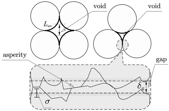
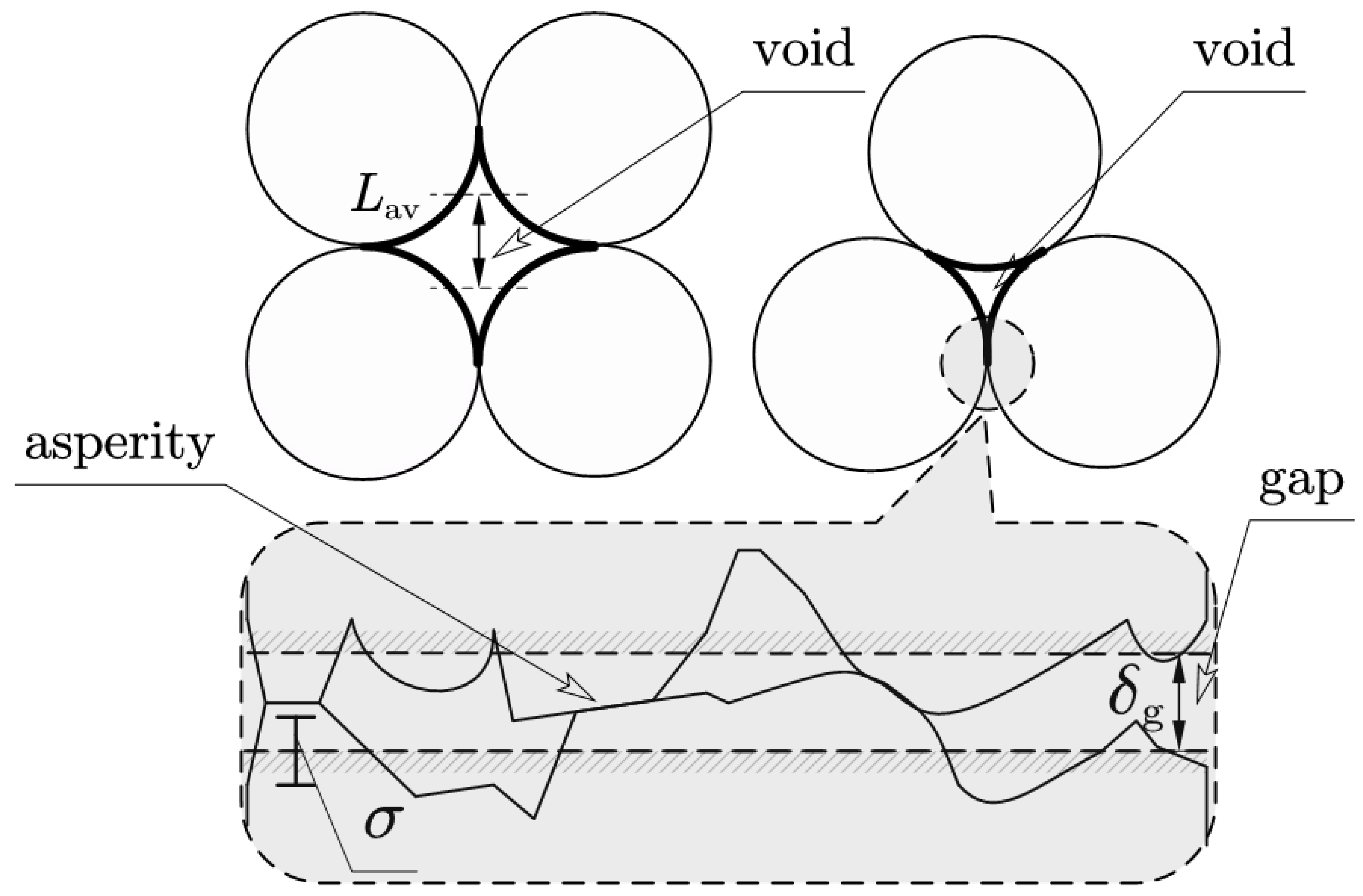
The comprehensive interlayer thermal resistance significantly influences the radial heat transfer characteristics of stranded conductors [18]. In the Morgan model, the interlayer thermal resistance of non-compacted stranded conductors is quantitatively decomposed into three components: the thermal resistance due to asperity contact at metallic interfaces, the thermal resistance associated with thin-layer air gaps between adjacent contact surfaces, and the thermal resistance attributable to air voids formed by wire stacking configurations. A schematic representation of these three heat transfer paths is illustrated in Figure 3.

Figure 3. Schematic illustration of the comprehensive interlayer thermal resistance of conductors.

Owing to the inherent surface roughness of metallic materials, heat conduction across the interface occurs through parallel pathways: solid conduction at asperity contact points and gaseous conduction across microscopic air gaps. Although the statistical distribution of asperities and gaps can, in principle, be characterized, its practical implementation in analytical models remains challenging. To facilitate engineering analysis, the rough contact interface is idealized as two parallel planes separated by a small distance, as indicated by the shaded dashed lines, where g represents the equivalent plane spacing and δ denotes the root-mean-square deviation of the rough surface profile from the reference plane. For the air voids situated at the centers of three-wire and four-wire stacking configurations, as highlighted by the thick lines, an equivalent heat conduction distance is introduced to transform the heat transfer problem from curved surfaces into an equivalent planar conduction model.

For compacted conductors, the stranding process substantially modifies each component of the comprehensive interlayer thermal resistance. Specifically, the elastoplastic deformation of asperities and substrates, accompanied by a concomitant reduction in air gap thickness, leads to significant alterations in both parameters g and δ. Furthermore, the compression of air voids necessitates a reformulation of the equivalent distance representation for curved surface heat transfer. Consequently, a comprehensive refinement of each component within the Morgan model framework is essential to accurately capture the thermal behavior of compacted stranded conductors.

2.2.1. Asperity Contact Heat Transfer on Metallic Contact Surfaces

In the Morgan model, which assumes that asperities in conductors undergo fully plastic deformation in a geometrical sense, the empirical formula for asperity contact heat conduction is given as follows [12]:

$$h_{\mathrm{mcon}}={\displaystyle \frac{1.13k_{\mathrm{hm}}\tan {\theta }_{\mathrm{m}}}{{\sigma }_{\mathrm{m}}}}{\left[{\displaystyle \frac{A_{\mathrm{r}}}{A_{\mathrm{a}}}}\right]}^{0.94}$$

(2)

where $h_{\mathrm{mcon}}$ represents the asperity contact thermal conductance; $k_{\mathrm{hm}}$ denotes the harmonic mean thermal conductivity of the contacting surfaces; $\tan {\mathsf{\theta }}_{\mathrm{m}}$ is the tangent of the mean slope angle of the asperities; ${\mathsf{\sigma }}_{\mathrm{m}}$ represents the standard deviation of the height relative to the equivalent plane; $A_{\mathrm{r}}$ is the real contact area of the metallic contact surface; and $A_{\mathrm{a}}$ is the apparent area of the metallic contact surface. Furthermore, this model assumes that deformation of wires is negligible, and that the asperity contact area ratio is linearly proportional to the contact pressure, i.e.,

$${\displaystyle \frac{A_{\mathrm{r}}}{A_{\mathrm{a}}}}={\displaystyle \frac{p_{\mathrm{q}}}{H}}$$

(3)

where $H$ is the microhardness of the metal, which is generally taken as three times the yield stress; $p_{\mathrm{q}}$ represents the average pressure over the apparent contact area, which is given by

$$p_{\mathrm{q}}={\displaystyle \frac{F^{\mathrm{rq}}}{A_{\mathrm{r}}}}$$

(4)

where $F^{\mathrm{rq}}$ denotes the radial force acting on the contact interface.

However, the deformation history of compacted conductors exhibits distinct characteristics that deviate from the assumptions underlying the conventional Morgan model. During the manufacturing stage, as the conductor passes through compacting dies, it is subjected to high pressure that induces substantial plastic deformation of the surface asperities. During the operational stage, the mechanical stress is substantially lower than that experienced during compaction. The contact interfaces undergo only elastic deformation, failing to maintain the intimate contact characteristic of fully plastic deformation. This “plastic-then-elastic” deformation sequence exhibits neither purely plastic nor purely elastic characteristics, deviating fundamentally from typical contact conditions.

Since the wires in compacted conductors have undergone significant geometric deformation during manufacturing, the influence of plastic flow on the asperity contact area must be explicitly considered. Pullen and Williamson [19] demonstrated that due to the plastic flow of the material, the asperity contact area ratio exhibits a nonlinear relationship with contact pressure that more closely approximates

$${\displaystyle \frac{A_{\mathrm{r}}}{A_{\mathrm{a}}}}={\displaystyle \frac{p_{\mathrm{q}}}{H+p_{\mathrm{q}}}}$$

(5)

Since the radial pressure on overhead insulated cables during operation cannot maintain the same tight contact characteristics as complete plastic deformation during manufacturing, the elastic deformation of the substrate beneath the asperities must be incorporated into the contact area formulation. Equation (5) is therefore modified to account for this elastic deformation of the substrate [20], yielding

$${\displaystyle \frac{A_{\mathrm{r}}}{A_{\mathrm{a}}}}={\displaystyle \frac{1}{1+2.5{\left(H/\left(E^{\prime }\tan {\theta }_{\mathrm{m}}\right)\right)}^{1.2}}}\cdot {\displaystyle \frac{p_{\mathrm{q}}}{H+p_{\mathrm{q}}}}$$

(6)

where $E^{\prime }$ is the combined elastic modulus of the two contacting wires, given by

$${\displaystyle \frac{1}{E^{\prime }}}={\displaystyle \frac{1-v_1^2}{E_1}}+{\displaystyle \frac{1-v_2^2}{E_2}}$$

(7)

where $E_1$ and $E_2$ represent the elastic moduli of the two metals, and $v_1$ and $v_2$ denote their Poisson’s ratios. The complete derivation of Equation (6) is given in Appendix A.3.

Substituting Equation (6) into Equation (2) yields the modified expression for asperity thermal contact conductance:

$$h_{\mathrm{mcon}}={\displaystyle \frac{1.13k_{\mathrm{hm}}\tan {\theta }_{\mathrm{m}}}{{\sigma }_{\mathrm{m}}}}{\left[{\displaystyle \frac{1}{1+2.5{\left(H/\left(E^{\prime }\tan {\theta }_{\mathrm{m}}\right)\right)}^{1.2}}}\cdot {\displaystyle \frac{p_{\mathrm{q}}}{H+p_{\mathrm{q}}}}\right]}^{0.94}.$$

(8)

Equation (8) quantitatively characterizes the influence of the “plastic-then-elastic” deformation behavior inherent to compacted conductors on asperity contact heat transfer, thereby capturing the essential physics of the contact interface under service conditions.

2.2.2. Heat Transfer Through Thin-Layer Air Gaps Between Metallic Contact Surfaces

The thermal conductance of thin-layer air gaps between metallic contact surfaces is given by

$$h_{\mathrm{gcon}}={\displaystyle \frac{k_{\mathrm{g}}}{{\delta }_{\mathrm{g}}}}$$

(9)

where $h_{\mathrm{gcon}}$ represents the thermal conductance of the thin-layer air gap; $k_{\mathrm{g}}$ denotes the thermal conductivity of air; and ${\mathsf{\delta }}_{\mathrm{g}}$ is the thickness of the air gap. It is evident that the thickness of the thin-layer air gap differs between compacted and non-compacted stranded conductors, making it a key parameter for characterizing the disparity in their heat transfer behavior. However, this thickness ${\mathsf{\delta }}_{\mathrm{g}}$ is difficult to measure directly or predict theoretically. In the Morgan model, empirical values are typically employed, for instance, the thin-layer air gap thickness for an aluminum–aluminum contact interface is taken as 1 × 10⁻⁶ m.

For compacted conductors, the air gap thickness is influenced by both the plastic flow of the metallic material and the elastic deformation of the substrate beneath the asperities. To enable quantitative analysis, an estimation formula for the thin-layer air gap thickness is derived herein. Based on the geometric deformation model, and under the assumptions that the heights of asperities follow a Gaussian distribution and the asperity slopes are randomly distributed, the analytical expression for the asperity contact area ratio is derived as follows:

$${\displaystyle \frac{A_{\mathrm{r}}}{A_{\mathrm{a}}}}={\displaystyle \frac{1}{2}}erfc\left({\displaystyle \frac{{\delta }_{\mathrm{g}}}{\sqrt{2}{\sigma }_{\mathrm{m}}}}\right)$$

(10)

Consequently, the thin-layer air gap thickness in compacted conductors can be derived by combining Equations (6) and (10):

$${\delta }_{\mathrm{g}}=\sqrt{2}\sigma \cdot erf{c}^{-1}\left({\displaystyle \frac{2}{1+2.5{\left(H/\left(E^{\prime }\tan \theta \right)\right)}^{1.2}}}\cdot {\displaystyle \frac{p_{\mathrm{q}}}{H+p_{\mathrm{q}}}}\right)$$

(11)

As indicated by Equations (4) and (6), the term $p_{\mathrm{q}}$ can be expressed accordingly:

$$p_{\mathrm{q}}={\displaystyle \frac{F^{\mathrm{rq}}+\sqrt{{\left(F^{\mathrm{rq}}\right)}^2+4\varphi A_{\mathrm{a}}{F}^{\mathrm{rq}}H}}{2A_{\mathrm{a}}\varphi }}$$

(12)

where $\varphi$ is defined as $1+2.5{\left(H/\left(E^{\prime }\tan {\mathsf{\theta }}_m\right)\right)}^{1.2}$. The apparent contact area $A_{\mathrm{a}}$ can be determined through calculation, which will be discussed in detail in subsequent sections.

2.2.3. Air Void Thermal Conductance

The thermal conductance of air voids is calculated by

$$h_{\mathrm{vcon}}=Nu\cdot {\displaystyle \frac{k_{\mathrm{g}}}{L_{\mathrm{av}}}}$$

(13)

where $Nu$ is the Nusselt number and $L_{\mathrm{av}}$ is the mean space. Due to the small volume of air voids and the minor temperature difference between adjacent wires, convective and radiative heat transfer can be neglected; thus, the Nusselt number is taken as $Nu=1$.

For compacted conductors, considering the reduction in air void size due to compression, and assuming for simplicity that the void shape remains unchanged while the area (volume) decreases, the approximate equivalent distances for triangular and quadrangular voids can be estimated based on the change in the void cross-sectional area:

$$L_{\mathrm{av}}^{\mathrm{tri}}=K_{\mathrm{C}}\left[{\displaystyle \frac{\sqrt{3}}{2}}-{\displaystyle \frac{\pi }{4}}\right]d$$

(14)

$$L_{\mathrm{av}}^{\mathrm{rec}}=K_{\mathrm{C}}\left[1-{\displaystyle \frac{\pi }{4}}\right]d$$

(15)

where the subscripts $\mathrm{tri}$ and $\mathrm{rec}$ denote triangular and quadrangular, respectively; $K_{\mathrm{C}}$ is the fill factor, expressed as follows:

$$K_{\mathrm{C}}=\sqrt{{\displaystyle \frac{\left(1-{\eta }_{\mathrm{com}}\right)A_{\mathrm{con}}^{\mathrm{com}}}{\left(1-{\eta }_{\mathrm{str}}\right)A_{\mathrm{con}}^{\mathrm{str}}}}}$$

(16)

where ${\mathsf{\eta }}_{\mathrm{com}}$ is the fill factor of the compacted conductor; ${\mathsf{\eta }}_{\mathrm{str}}$ is the theoretical fill factor of the stranded conductor; $A_{\mathrm{con}}^{\mathrm{com}}$ is the contour area of the compacted conductor; $A_{\mathrm{con}}^{\mathrm{str}}$ is the contour area of the stranded conductor; and $d$ is the diameter of a wire.

2.3. Interlayer Contact Area

The thermal resistance between layer i − 1 and layer i is given by

$$R_{\left(i-1\right)i}^{\mathrm{T}}={\displaystyle \frac{1}{{\left(h_{\mathrm{mcon}}{A}_{\mathrm{m}}+h_{\mathrm{gcon}}{A}_{\mathrm{g}}+h_{\mathrm{vcon}}{A}_{\mathrm{v}}\right)}_{\left(i-1\right)i}}}$$

(17)

where $A_{\mathrm{m}}$, $A_{\mathrm{g}}$ and $A_{\mathrm{v}}$ are the areas associated with the asperity contact, thin-layer air gap, and air voids, respectively, between the layers. These areas depend on the radial forces within the conductor. Generally, tighter compression (higher radial force) leads to a larger asperity contact area, smaller and thinner air gap, and smaller air voids. Therefore, reasonably estimating the radial stress generated between conductor layers during cable operation is crucial.

2.3.1. Radial Stress Analysis

The following assumptions are adopted to facilitate the analysis: (1) the stress along its own axis is the same for individual wires of the same material; (2) changes in lay angle due to stress are neglected.

The axial forces on the aluminum and steel components are

$$f_{\mathrm{al}}^{\mathrm{con}\text{-}\mathrm{a}}={\displaystyle \frac{F-\left({\chi }_{\mathrm{al}}-{\chi }_{\mathrm{st}}\right)\Delta T{A}_{\mathrm{st}}{E}_{\mathrm{st}}}{A_{\mathrm{al}}{E}_{\mathrm{al}}+A_{\mathrm{st}}{E}_{\mathrm{st}}}}\times E_{\mathrm{al}}$$

(18)

$$F_{\mathrm{al}}^{\mathrm{con}\text{-}\mathrm{a}}=f_{\mathrm{al}}^{\mathrm{con}\text{-}\mathrm{a}}{A}_{\mathrm{al}}$$

(19)

$$F_{\mathrm{st}}^{\mathrm{con}\text{-}\mathrm{a}}=F-F_{\mathrm{al}}^{\mathrm{con}\text{-}\mathrm{a}}$$

(20)

where $f_{\mathrm{a}\mathrm{l}}^{\mathrm{c}\mathrm{o}\mathrm{n}-\mathrm{a}}$ is the axial stresses in the aluminum wires along the conductor axis; $F$ is the total axial tension on the conductor;$F_{\mathrm{a}\mathrm{l}}^{\mathrm{c}\mathrm{o}\mathrm{n}-\mathrm{a}}$ and $F_{\mathrm{s}\mathrm{t}}^{\mathrm{c}\mathrm{o}\mathrm{n}-\mathrm{a}}$ are the axial forces in the aluminum and steel components, respectively; $A_{\mathrm{al}}$ and $A_{\mathrm{st}}$ are the cross-sectional areas of the aluminum and steel components; ${\chi }_{\mathrm{al}}$ and ${\chi }_{\mathrm{st}}$ are the coefficients of thermal expansion; $E_{\mathrm{al}}$ and $E_{\mathrm{st}}$ are the elastic moduli; and $\mathsf{\Delta }T$ is the temperature difference from the installation temperature.

Based on assumption (1), the stresses along the axis of individual wires in the steel portion and aluminum portion are calculated respectively:

$$F_{\mathrm{st}}^{\mathrm{con}\text{-}\mathrm{a}}={\displaystyle \frac{\pi f_{\mathrm{st}}^{\mathrm{wire}\text{-}\mathrm{a}}}{4}}(n_0{d}_0^2{\cos }^3{\beta }_0+n_1{d}_1^2{\cos }^3{\beta }_1+\cdots +n_i{d}_i^2{\cos }^3{\beta }_i)$$

(21)

$$F_{\mathrm{al}}^{\mathrm{con}\text{-}\mathrm{a}}={\displaystyle \frac{\pi f_{\mathrm{al}}^{\mathrm{wire}\text{-}\mathrm{a}}}{4}}(n_{i+1}{d}_{i+1}^2{\cos }^3{\beta }_{i+1}+n_{i+2}{d}_{i+2}^2\cdot {\cos }^3{\beta }_{i+2}+\cdots +n_{i+j}{d}_{i+j}^2{\cos }^3{\beta }_{i+j})$$

(22)

where $f_{\mathrm{al}}^{\mathrm{wire}\text{-}\mathrm{a}}$ is the stress along its own axis of an aluminum wire; $f_{\mathrm{st}}^{\mathrm{wire}\text{-}\mathrm{a}}$ is the stress along its own axis of a steel wire; ${\beta }_i$ is the lay angle of the i-th layer conductor; $d_i$ is the diameter of wires in the i-th layer conductor; and $n_i$ is the number of wires in the i-th layer conductor.

Substitute Equations (18)–(20) into Equations (21) and (22) respectively, and $f_{\mathrm{al}}^{\mathrm{wire}\text{-}\mathrm{a}}$ and $f_{\mathrm{st}}^{\mathrm{wire}\text{-}\mathrm{a}}$ can be solved. Then, the total force acting along the conductor axis of all wires in the i-th layer conductor $F_i^{\mathrm{con}\text{-}\mathrm{a}}$ can be calculated as follows:

$$F_i^{\mathrm{con}\text{-}a}={\displaystyle \frac{n_i\pi d_i^2}{4}}{f}_i^{\mathrm{wire}\text{-}\mathrm{a}}{\cos }^2{\beta }_i$$

(23)

where $f_{\mathrm{i}}^{\mathrm{wire}\text{-}\mathrm{a}}$ belongs to set $\left\{f_{\mathrm{al}}^{\mathrm{wire}\text{-}\mathrm{a}}, f_{\mathrm{st}}^{\mathrm{wire}\text{-}\mathrm{a}}\right\}$.

Then, the radial pressure generated by the i-th layer conductor is

$$F_i^{\mathrm{con}\text{-}\mathrm{r}}={\displaystyle \frac{F_i^{\mathrm{con}\text{-}\mathrm{a}}{\sin }^2{\beta }_i}{i{d}_i}}$$

(24)

The total radial pressure acting on the i-th layer conductor is

$${\overline{F}}_i^{\mathrm{r}}={\displaystyle \sum _{j=i+1}^N{F}_j^{\mathrm{con}\text{-}\mathrm{r}}}$$

(25)

where $N$ represents the total number of the layers.

2.3.2. Contact Area Estimation

The number $q_{\left(i-1\right)i}$ of asperity contacts per unit length between wires in layer i − 1 and layer i is

$$q_{\left(i-1\right)i}=n_{i-1}^2\left({\displaystyle \frac{1}{s_{i-1}}}+{\displaystyle \frac{1}{s_i}}\right)$$

(26)

where $s_i$ represents the pitch of the wires in the i-th layer; in particular, ${\mathrm{q}}_{01}=6/{\mathrm{s}}_1$.

The radial force per contact in layer i − 1 is

$$F_{i-1}^{\mathrm{rq}}={\displaystyle \frac{{\overline{F}}_{i-1}^{\mathrm{r}}}{q_{\left(i-1\right)i}}}$$

(27)

Thus, the apparent area of each contact between layer i − 1 and layer i is

$$A_{\left(i-1\right)i}^{\mathrm{q}}={\displaystyle \frac{F_{i-1}^{\mathrm{rq}}}{\min \left\{f_{\mathrm{y},i-1},f_{\mathrm{y},i}\right\}}}$$

(28)

where $\mathrm{m}\mathrm{i}\mathrm{n}\left\{{\mathrm{f}}_{\mathrm{y},\mathrm{i}-1},{\mathrm{f}}_{\mathrm{y},\mathrm{i}}\right\}$ represents the smaller yield stress of the two metals in layer i − 1 and layer i.

The apparent contact area of the total metal asperities between layer i − 1 and layer i is

$$A_{\mathrm{a},\left(i-1\right)i}=q_{\left(i-1\right)i}{A}_{\left(i-1\right)i}^{\mathrm{q}}$$

(29)

In summary, the expressions for $A_{\mathrm{m},\left(i-1\right)i}$, $A_{\mathrm{g},\left(i-1\right)i}$, and $A_{\mathrm{v},\left(i-1\right)i}$ are

$$A_{\mathrm{m},\left(i-1\right)i}=q_{\left(i-1\right)i}{A}_{\left(i-1\right)i}^q{\displaystyle \frac{A_{\mathrm{r}}}{A_{\mathrm{a}}}}$$

(30)

$$A_{\mathrm{g},\left(i-1\right)i}=q_{\left(i-1\right)i}{A}_{\left(i-1\right)i}^q\left(1-{\displaystyle \frac{A_{\mathrm{r}}}{A_{\mathrm{a}}}}\right)$$

(31)

$$A_{\mathrm{v},\left(i-1\right)i}=\pi d_{i-1}\left(2i-1\right)-q_{\left(i-1\right)i}{A}_{\left(i-1\right)i}^q$$

(32)

3. Calculation Procedure for Current–Temperature Relationship

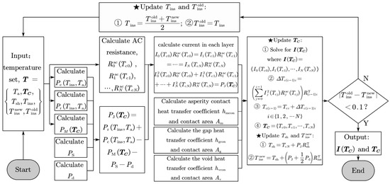
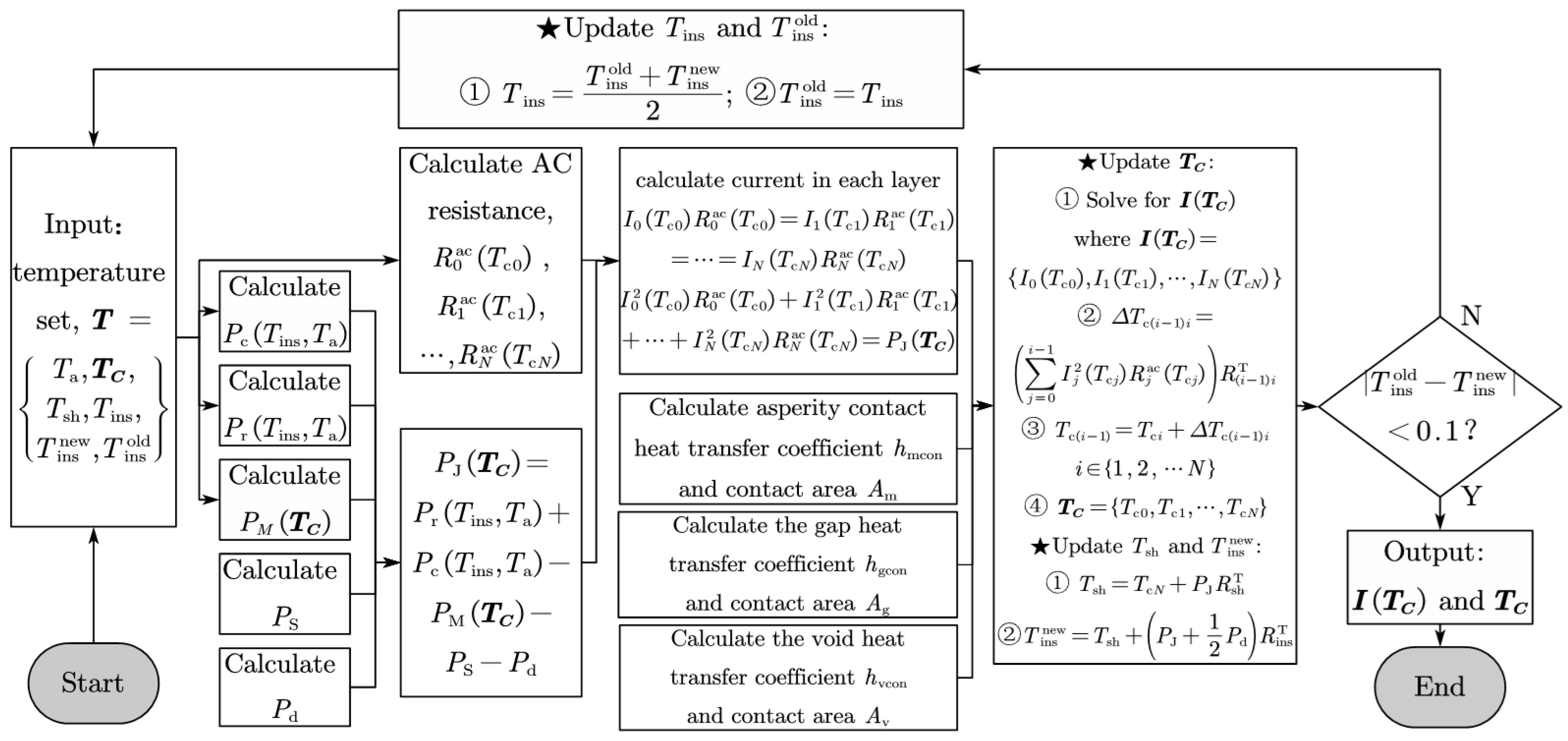
To determine the insulation outer surface temperature accurately, an iterative solution procedure is designed in this study, as illustrated in Figure 4. The Joule loss of a conductor layer is expressed as follows:

$$P_{\mathrm{J}}\left(T_C\right)={\displaystyle \sum _{i=0}^N{I}_i^2\left(T_{\mathrm{c}i}\right)R_i^{\mathrm{ac}}\left(T_{\mathrm{c}i}\right)}$$

(33)

where $I_{\mathrm{c}i}$ is the current in the i-th layer of the conductor; $R_i^{\mathrm{ac}}$ is the AC resistance of the i-th layer; ${\mathit{T}}_{\mathit{C}}$ is the collection of temperature in the conductor layers; and $T_{\mathrm{c}i}$ denotes the conductor temperature in the i-th layer conductor and $T_{\mathrm{c}i}\in {\mathit{T}}_{\mathit{C}}$.

Figure 4. Flowchart for calculating the ampacity of overhead insulated cables. The pentagram symbol indicates the temperature update step in the iterative cycle.

The current distribution among conductor layers follows Ohm’s law for parallel conductors:

$$I_0\left(T_{\mathrm{c}0}\right)R_0^{\mathrm{ac}}\left(T_{\mathrm{c}0}\right)=\cdots =I_i\left(T_{\mathrm{c}i}\right)R_i^{\mathrm{ac}}\left(T_{\mathrm{c}i}\right)=\cdots =I_N\left(T_{\mathrm{c}N}\right)R_N^{\mathrm{ac}}\left(T_{\mathrm{c}N}\right)$$

(34)

Accurate determination of ${\mathrm{R}}_{\mathrm{i}}^{\mathrm{ac}}\left(T_{\mathrm{c}i}\right)$ is therefore critical. Considering the influence of the skin effect on AC resistance, the AC resistance of the i-th layer conductor at temperature ${\mathrm{T}}_{\mathrm{c}i}$ is

$$R_i^{\mathrm{ac}}\left(T_{\mathrm{c}i}\right)=k_i^{\mathrm{sk}}\cdot R_i^{\mathrm{dc}}(20)\left(1+{\alpha }_{20}\left(T_{\mathrm{c}i}-20\right)+{\zeta }_{20}{\left(T_{\mathrm{c}i}-20\right)}^2\right)$$

(35)

where $k_i^{\mathrm{sk}}$ is the skin effect factor for the i-th layer conductor; $R_i^{\mathrm{dc}}$ is the DC resistance of the i-th layer conductor at 20 °C; and ${\mathsf{\alpha }}_{20}$ and ${\mathsf{\zeta }}_{20}$ are the linear and quadratic resistance temperature coefficients at 20 °C.

For simplicity, a uniform skin effect factor is applied to each layer of the homogeneous conductor. For the ACSR core in an overhead insulated cable, two distinct skin effect factors are employed for the aluminum strands and the steel strands, respectively.

The skin effect factor [8] is given by

$$\left\{\begin{array}{l}{k}_{\mathrm{hom}\mathrm{o}}^{\mathrm{sk}}\left(D_{\mathrm{od}}\right)={\displaystyle \frac{D_{\mathrm{od}}^2\cdot \pi }{4\rho }}\mathrm{Re}\mathrm{al}\left[{\displaystyle \frac{\rho \cdot \left(1-1j\right)}{D_{\mathrm{od}}\cdot \pi \cdot {\delta }_{\mathrm{sk}}}}\cdot {\displaystyle \frac{J_0}{J_1}}\right]\\ k_{\mathrm{tube}}^{\mathrm{sk}}\left(D_{\mathrm{od}},D_{\mathrm{id}}\right)=1+\left(k_{\mathrm{hom}\mathrm{o}}^{\mathrm{sk}}\left(D_{\mathrm{od}}\right)-1\right)\cdot \left(1-{\displaystyle \frac{D_{\mathrm{id}}}{D_{\mathrm{od}}}}\right)\\ J_0\left(x\right)=1-{\left({\displaystyle \frac{x}{2}}\right)}^2+{\displaystyle \frac{1}{4}}{\left({\displaystyle \frac{x}{2}}\right)}^4-{\displaystyle \frac{1}{36}}{\left({\displaystyle \frac{x}{2}}\right)}^6\\ J_1\left(x\right)={\displaystyle \frac{x}{2}}-{\displaystyle \frac{1}{2}}{\left({\displaystyle \frac{x}{2}}\right)}^3+{\displaystyle \frac{1}{12}}{\left({\displaystyle \frac{x}{2}}\right)}^5-{\displaystyle \frac{1}{144}}{\left({\displaystyle \frac{x}{2}}\right)}^7\\ x={\displaystyle \frac{\left(1-1j\right)\cdot D_{\mathrm{od}}}{2\cdot {\delta }_{\mathrm{sk}}}}\\ {\delta }_{\mathrm{sk}}=\sqrt{{\displaystyle \frac{\rho }{4f{\pi }^2{\mu }_r\cdot {10}^{-7}}}}\end{array}\right.$$

(36)

where $k_{\mathrm{homo}}^{\mathrm{sk}}$ is the skin effect factor for a homogeneous cylindrical stranded conductor; $k_{\mathrm{tube}}^{\mathrm{sk}}$ is the skin effect factor for a tubular stranded conductor; $D_{\mathrm{od}}$ is the outer diameter of the stranded conductor; $D_{\mathrm{id}}$ is the inner diameter of the tubular stranded conductor; ${\mathsf{\delta }}_{\mathrm{sk}}$ is the skin depth; $J_0$ and $J_1$ are the 0th-order and first-order Bessel functions of the first kind; $x$ is the variable of the Bessel function; $f$ is the frequency; $\mathsf{\rho }$ is the resistivity of the metal; and ${\mathsf{\mu }}_r$ is its relative permeability.

The DC resistance of the i-th layer conductor at 20 °C can be written as

$$R_i^{\mathrm{dc}}\left(20\right)={\displaystyle \frac{4{\rho }_{20,i}\sqrt{1+{\left(\pi D_i/s_i\right)}^2}}{\pi d_i^2\cdot n_i}}$$

(37)

where $D_i$ is the diameter of the i-th layer and ${\mathsf{\rho }}_{20,i}$ is the resistivity of the i-th layer conductor at 20 °C.

The Joule loss of the conductor can be described by the heat balance equation:

$$P_{\mathrm{J}}\left(T_C\right)=P_{\mathrm{r}}\left(T_{\mathrm{ins}},T_{\mathrm{a}}\right)+P_{\mathrm{c}}\left(T_{\mathrm{ins}},T_{\mathrm{a}}\right)-P_{\mathrm{M}}\left(T_C\right)-P_{\mathrm{S}}-P_{\mathrm{d}}$$

(38)

For brevity, the forced convective heat loss $P_{\mathrm{c}}\left(T_{\mathrm{ins}},T_{\mathrm{a}}\right)$ is detailed in Appendix A.2.1; the radiated heat loss $P_{\mathrm{r}}\left(T_{\mathrm{ins}},T_{\mathrm{a}}\right)$ in Appendix A.2.2; the solar gain $P_{\mathrm{S}}$ in Appendix A.2.3; and the dielectric loss $P_{\mathrm{d}}$ in Appendix A.2.4. The calculation method for $P_{\mathrm{M}}\left(T_C\right)$ is specified in CIGRE TB 345.

By combining Equations (33), (34) and (38), and employing the thermal circuit model illustrated in Figure 2, the temperatures at the conductor shield outer surface and insulation outer surface can be derived sequentially:

$$T_{\mathrm{sh}}=T_{\mathrm{c}N}+P_{\mathrm{J}}{R}_{\mathrm{sh}}^{\mathrm{T}}$$

(39)

$$T_{\mathrm{ins}}^{\mathrm{new}}=T_{\mathrm{sh}}+\left(P_{\mathrm{J}}+{\displaystyle \frac{1}{2}}{P}_{\mathrm{d}}\right)R_{\mathrm{ins}}^{\mathrm{T}}$$

(40)

where $T_{\mathrm{c}N}$ is the outermost conductor layer temperature, typically taken as the permissible operating temperature of 90 °C; $T_{\mathrm{i}\mathrm{n}\mathrm{s}}^{\mathrm{n}\mathrm{e}\mathrm{w}}$ is the insulation outer surface temperature obtained from this iteration cycle.

The updated insulation outer surface temperature modifies the temperature distribution across the conductor layers, which in turn affects the AC resistance losses. This coupled relationship necessitates an iterative solution scheme:

$$\begin{array}{l}{T}_{\mathrm{ins}}={\displaystyle \frac{T_{\mathrm{ins}}^{\mathrm{old}}+T_{\mathrm{ins}}^{\mathrm{new}}}{2}} \\ T_{\mathrm{ins}}^{\mathrm{old}}=T_{\mathrm{ins}}\end{array}$$

(41)

The iteration proceeds until convergence is achieved:

$$\left|T_{\mathrm{ins}}^{\mathrm{old}}-T_{\mathrm{ins}}^{\mathrm{new}}\right|<0.1 ℃$$

(42)

4. Method Validation

The feasibility and accuracy of the proposed model are validated using the JKLGYJ 240/30 overhead insulated cable. This compacted conductor has a fill factor of 0.84, with aluminum and steel wire diameters of 3.64 mm and 2.40 mm, respectively.

4.1. Convergence Validation

To assess the convergence behavior of the proposed iterative procedure, a typical operating condition was selected for iterative calculation: ambient temperature of 40 °C, wind speed of 0.2 m/s (close to natural convection), and conductor stress of 7 kN. Following the procedure shown in Figure 4, the initial temperature of each conductor layer was set to 90 °C, and the initial insulation outer surface temperature was set to 70 °C. Convergence was judged according to Equation (42).

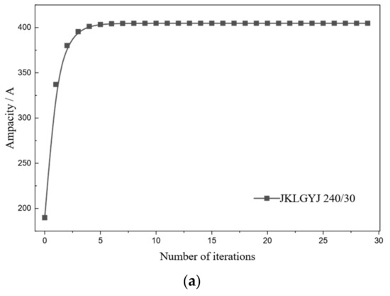
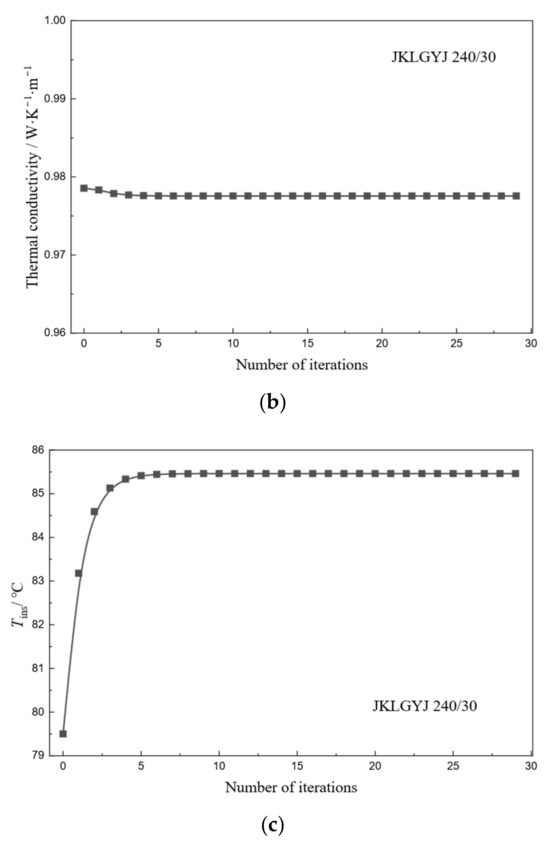
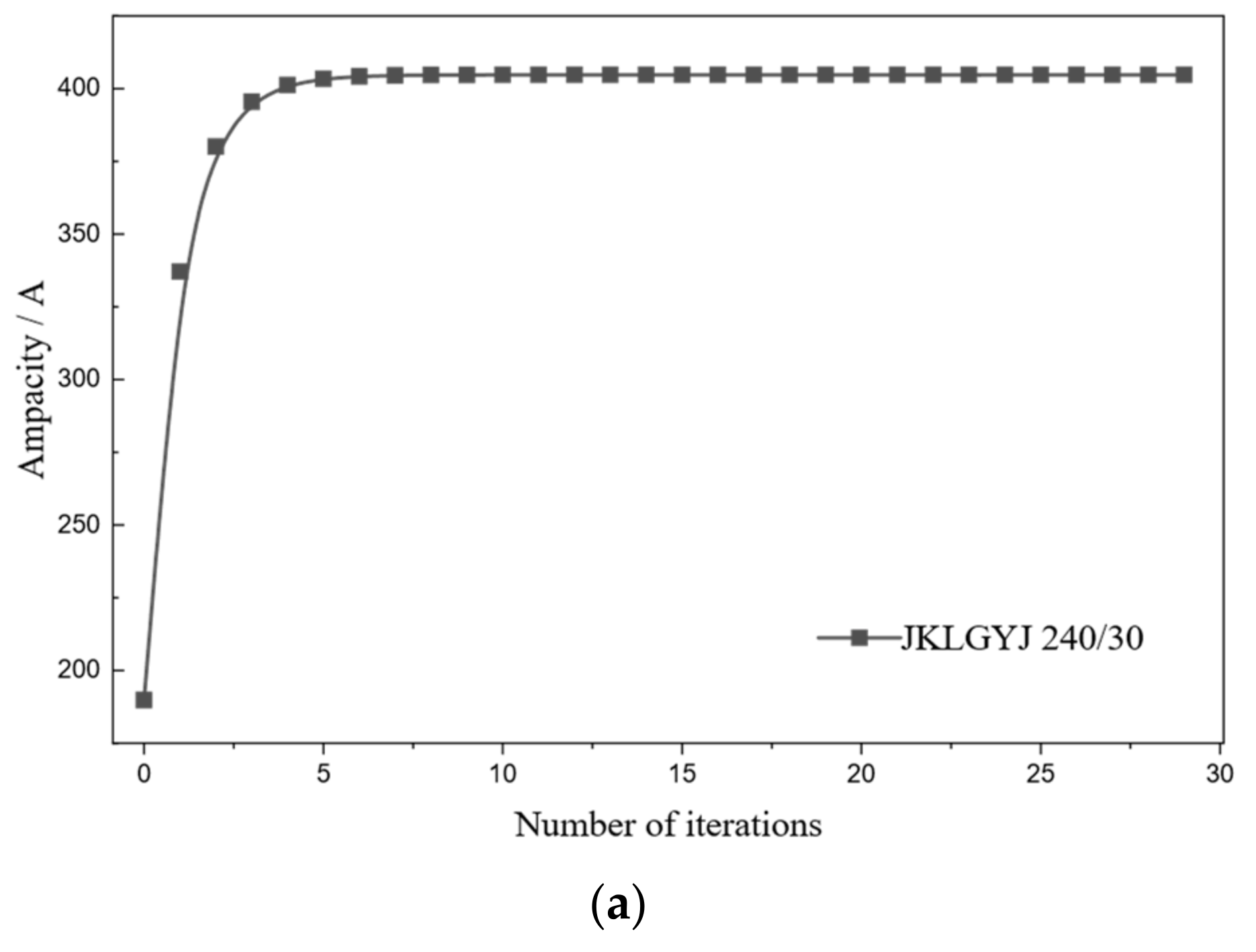
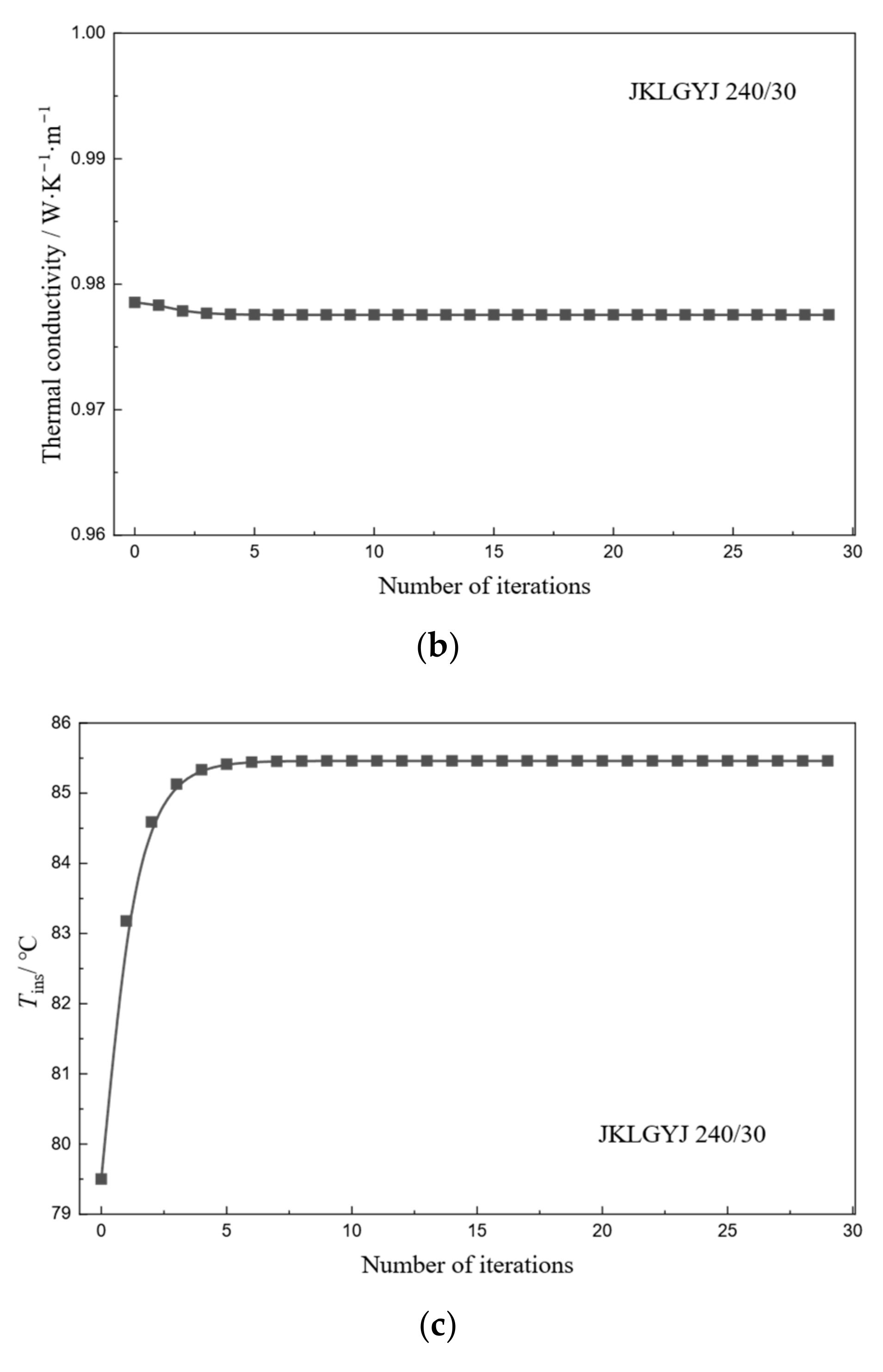
Figure 5 shows the convergence process over 30 iteratives. Under the specified conditions, the ampacity of JKLGYJ 240/30 converges to 404.7 A (Figure 5a), the equivalent radial thermal conductivity to 0.98 W/(m·K) (Figure 5b), and the insulation outer surface temperature to 85.8 °C (Figure 5c). All three parameters stabilize after six iterations, indicating that the method has good convergence and feasibility.

Figure 5. Iterative convergence process of ampacity, thermal conductivity and outer surface temperature of the insulation layer. (a) Iterative convergence process of ampacity; (b) iterative convergence process of thermal conductivity; (c) iterative convergence process of outer surface temperature of the insulation layer.

4.2. Accuracy Validation

To verify the accuracy of the proposed model, radial temperature difference measurements were conducted on the compacted conductor using a current generation device and a wind tunnel test platform [13]. The experimental results were compared with the calculated results from the Morgan model and the improved model presented herein.

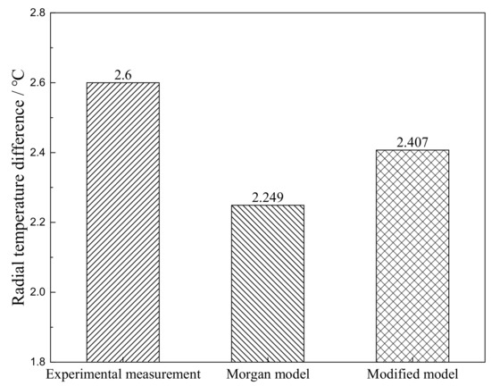
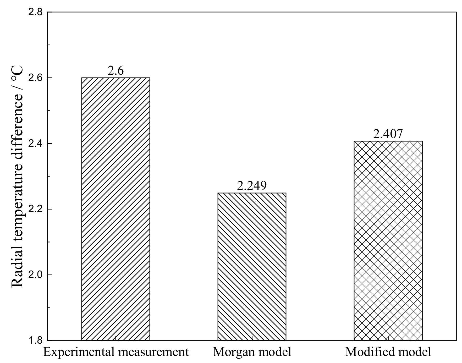
The test conditions were set as follows: sample cable length of 2 m, ambient temperature of 26 °C, conductor stress of 7 kN, and wind speed of 0.5 m/s directed horizontally and perpendicular to the conductor axis. Four temperature sensors are installed between each layer, positioned at the windward, leeward, upper, and lower sides of the conductor. Under an applied current of 450 A, the measured radial temperature difference and the corresponding calculated values are presented in Figure 6. The measured radial temperature difference in the compacted conductor is 2.6 °C. The Morgan model yields a calculated value of 2.249 °C, while the proposed model gives 2.407 °C. The improved model demonstrates better agreement with the experimental results, exhibiting significantly higher accuracy than the conventional Morgan model. The average temperature of each conductor layer is provided in Appendix B.1.

Figure 6. Radial temperature difference in JKLGYJ 240/30 overhead insulated cable.

The validation results confirm that the proposed model accurately captures the thermal behavior of compacted conductors. The iterative solution converges rapidly, with all key parameters stabilizing within six iterations. The calculated radial temperature difference agrees closely with the measured value, yielding an error of 7.4%, significantly lower than the 13.5% error of the conventional Morgan model. This improved accuracy stems from incorporating the distinctive deformation characteristics of compacted conductors into the formulations for asperity contact, thin-layer air gaps, and air voids: namely, plastic deformation during manufacturing and elastic recovery under service tension. These refinements provide a more physically representative description of the radial temperature distribution, thereby validating the theoretical framework established in Section 2.

5. Ampacity Characteristics Analysis

Based on the radial heat transfer model of compacted conductors and the iterative solution method established in the previous sections, this section selects two types of overhead insulated cables with typical structures to systematically analyze the influence patterns of key factors such as the ambient temperature, conductor stress, and wind speed on the ampacity, revealing the thermal behavior characteristics of compacted conductors under different operating conditions.

5.1. Input Conditions

5.1.1. Types and Specifications of Overhead Insulated Cables

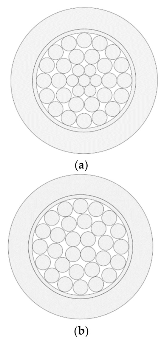
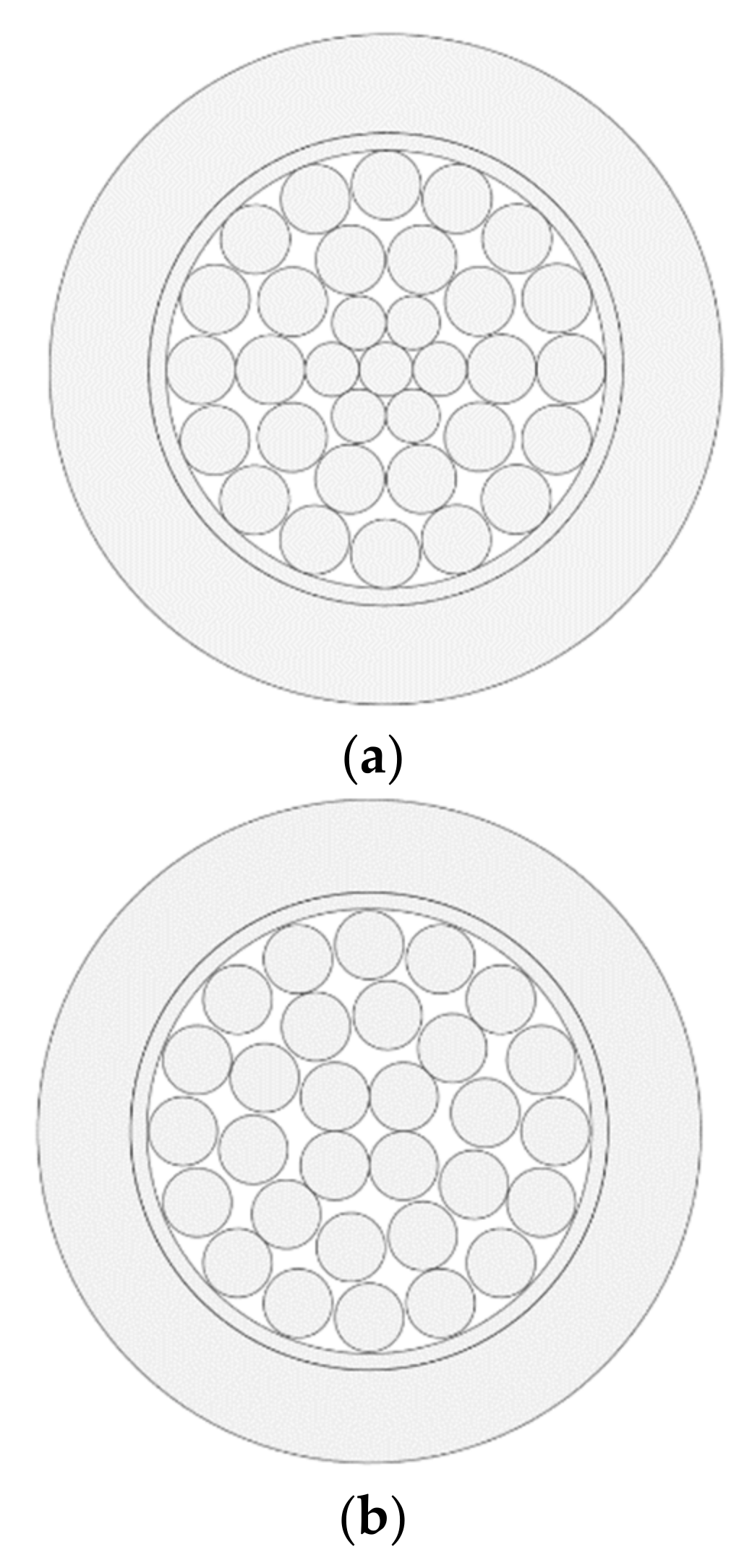
To investigate the thermal behavior of overhead insulated cables with compacted conductors under different operating conditions and its influence on the ampacity, this paper selects two types of overhead insulated cables with different models but similar specifications as calculation objects, with their structures shown in Figure 7. One is the aluminum conductor steel-reinforced core cable JKLGYJ 120/20, with the compacted conductor following the recommended structure in GB 1179 [21], where individual wires are arranged in a 1 + 6 + 12 + 18 configuration, as shown in Figure 7a. The other is the aluminum alloy core cable JKLHYJ 150, with the compact structure complying with the provisions of GB 14049 [22], where individual wires are arranged in a 4 + 10 + 16 configuration, as shown in Figure 7b. Table 1 summarizes the detailed parameters of the relevant cable structures.

Figure 7. Schematic diagram of overhead insulated cable structures. (a) JKLGYJ 120/20; (b) JKLHYJ 150.

Table 1. Structural parameters for overhead insulated cables.

Type & Size	Single-Wire Diameter/mm	Conductor Outer Diameter/mm	Shielded Outer Diameter/mm	Insulation Outer Diameter/mm
JKLGYJ 120/20	1.85/ 2.45	5.55/ 13.77	14.97	21.77
JKLHYJ 150	2.54	15.08	16.28	23.08

5.1.2. Geographical and Meteorological Conditions

The case study line in this paper is a 10 kV overhead transmission line in a certain area of Sichuan Province, with an average span of approximately 80 m. According to meteorological records from the past 10 years, this region is classified under the Type A typical meteorological zone [23]. Based on this, the environmental and meteorological parameters are compiled, as shown in Table 2.

Table 2. Geographical environment and meteorological parameters.

Item	Parameter	Value
①	Maximum ambient temperature/°C	40
②	Annual average ambient temperature/°C	20
③	High wind environmental temperature/°C	10
④	Average wind speed/m·s−1	2
⑤	Maximum wind speed/m·s−1	20
⑥	Minimum wind speed/m·s−1	0.2
⑦	Altitude $y$/m	500
	Latitude $\mathsf{\phi }$/deg	28.5
	Solar declination ${\mathsf{\delta }}_{\mathrm{S}}$/deg	23.0
	Atmospheric clarity $N_{\mathrm{S}}$	1.0
	Solar azimuth $Z$/deg	15.5
	Azimuth of the conductor ${\gamma }_{\mathrm{C}}$/deg	45.0
	Absorptivity of insulation ${\alpha }_{\mathrm{S}}$	0.8
	Reflectance of the ground ${\mathrm{F}}_{\mathrm{R}}$	0.15
	Emissivity of the insulating surface ${\epsilon }_{\mathrm{S}}$	0.8
	Angle between the wind direction and the conductor axis/deg	90

To comprehensively evaluate the ampacity characteristics under different operating conditions, three typical meteorological conditions are combined based on the parameters in Table 2: 100% load conditions (① + ⑥ + ⑦), average annual meteorological conditions (② + ④ + ⑦), and high-wind meteorological conditions (③ + ⑤ + ⑦), representing the conditions with the highest conductor thermal load, the longest operating time, and the strongest heat dissipation capacity, respectively.

5.2. Influence of Ambient Temperature on Ampacity

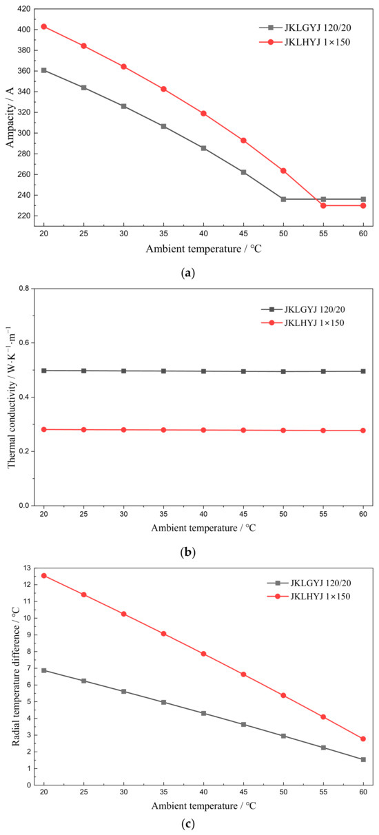
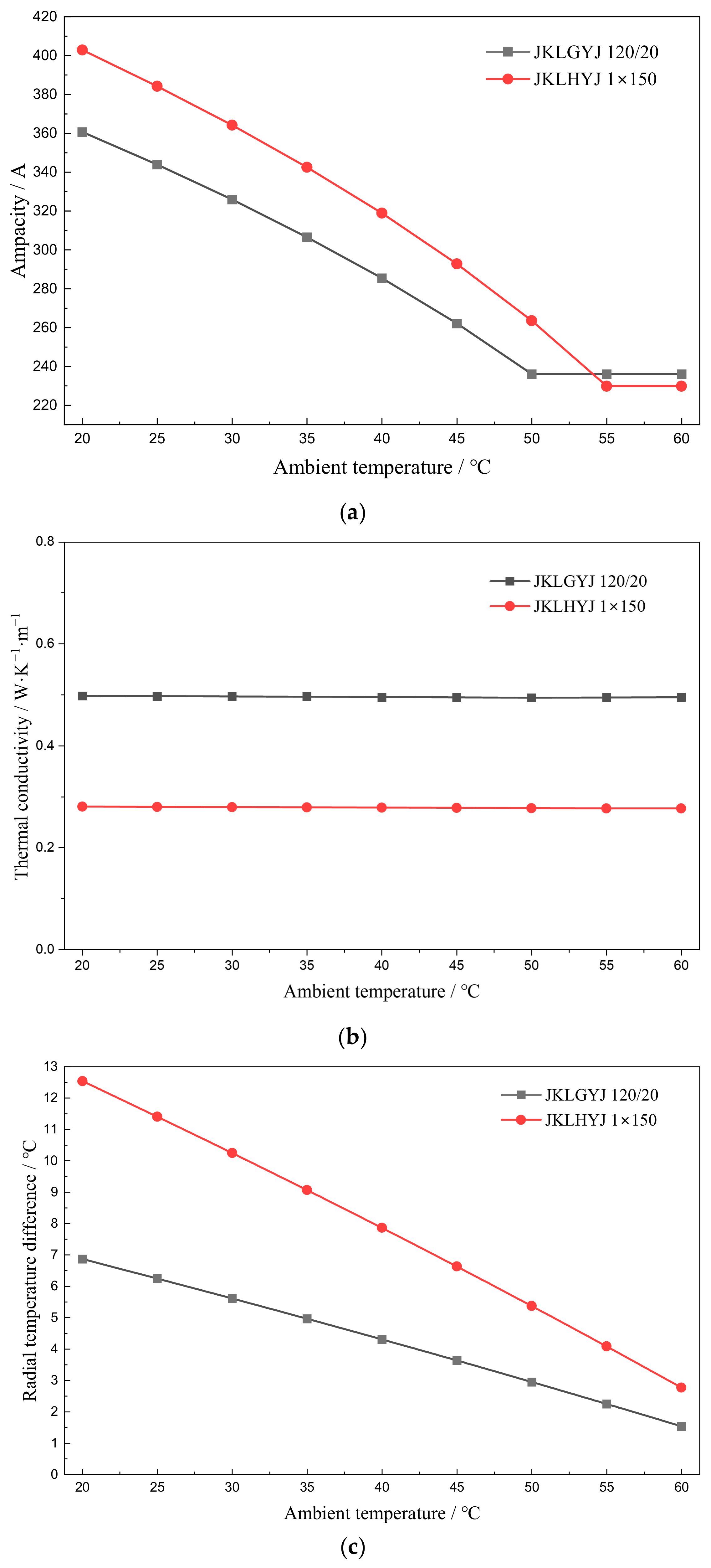
Ambient temperature is a fundamental factor affecting the heat dissipation capacity of conductors, and its influence on the ampacity is most significant under the most severe operating conditions. Therefore, the 100% load conditions are selected for analysis. Under these conditions, the conductor temperature approaches the upper limit of the allowable operating temperature, which can fully reveal the coupling relationship between the ambient temperature and ampacity. Figure 8 shows the variation patterns of the ampacity, equivalent radial thermal conductivity, and conductor radial temperature difference with ambient temperature for the two types of compacted conductor overhead insulated cables under these conditions.

Figure 8. Comparison of ampacity, equivalent radial thermal conductivity, and radial temperature difference under different ambient temperatures. (a) Variation in ampacity with ambient temperature; (b) variation in equivalent radial thermal conductivity with ambient temperature; (c) variation in radial temperature difference with ambient temperature.

As shown in Figure 8a, the ampacity of both cable types decreases with the increasing ambient temperature. When the ambient temperature is low, the conductor dissipates heat adequately, resulting in a higher ampacity; as the ambient temperature increases, the heat dissipation capacity decreases, and the ampacity decreases correspondingly. When the ambient temperature approaches the conductor operating temperature, heat dissipation is hindered, and the decrease in the ampacity slows down, exhibiting a “tail phenomenon.” This indicates that when the conductor approaches its thermal equilibrium limit, the sensitivity of the ampacity to ambient temperature decreases. Comparing the two cables, the ampacity of JKLHYJ 150 is higher than that of JKLGYJ 120/20, reflecting the current-carrying advantage of aluminum alloy conductors, which is closely related to the resistance-temperature characteristics of the material and the conductor structure.

Figure 8b shows that changes in ambient temperature have essentially no effect on the equivalent radial thermal conductivity of the two cable conductors, indicating that the radial heat transfer performance of the conductor is independent of the ambient temperature. JKLGYJ 120/20 exhibits better radial heat transfer performance than JKLHYJ 150 under the same conditions. This may be because the central layer of JKLHYJ 150 consists of four conductors, and both its single-wire diameter and conductor diameter are larger than those of JKLGYJ 120/20. Consequently, the structure of JKLHYJ 150 is more sparse, resulting in higher interlayer contact thermal resistance. Additional simulation results supporting this conclusion are presented in Appendix B.2. This phenomenon validates the previous theoretical analysis regarding the influence of the fill factor on the equivalent distance of air voids.

As the ambient temperature increases, the radial temperature difference in both conductors gradually decreases, as shown in Figure 8c. This indicates that the radial temperature difference is not only affected by the internal heat transfer characteristics of the conductor but also closely related to the external heat dissipation conditions. Under the premise that the equivalent radial thermal conductivity remains unchanged, an increase in the ambient temperature weakens the temperature difference driving force between the conductor and the external environment, reducing the heat dissipation capacity and thereby leading to a decrease in the radial temperature difference.

5.3. Influence of Conductor Stress on Radial Temperature Difference and Ampacity

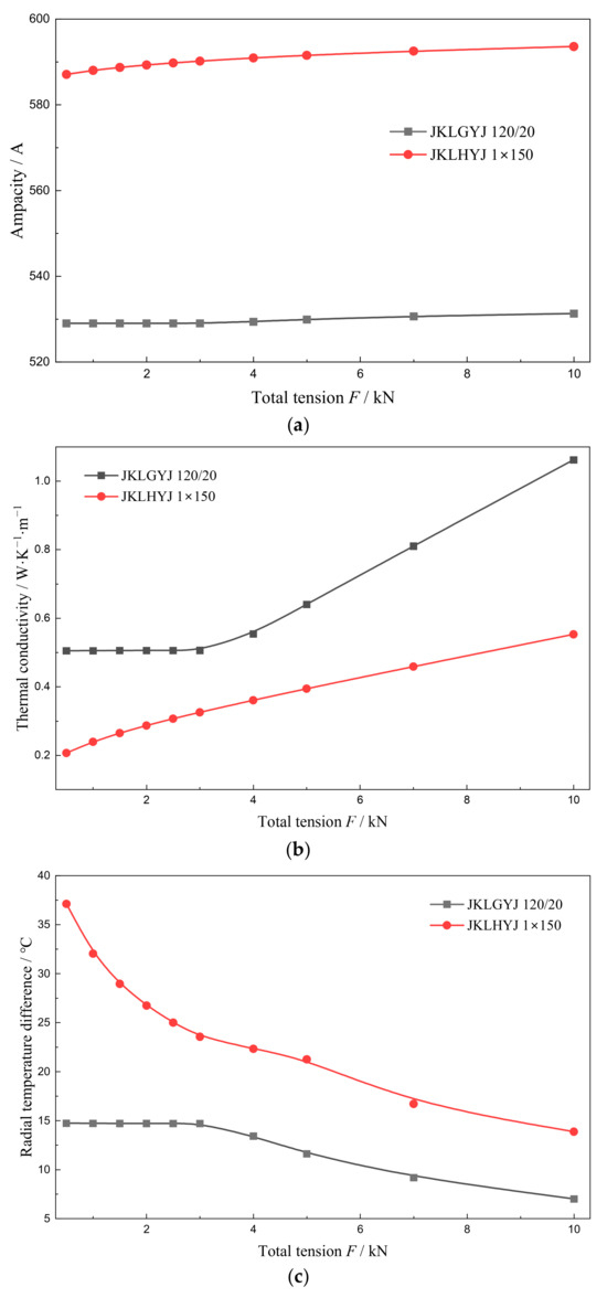
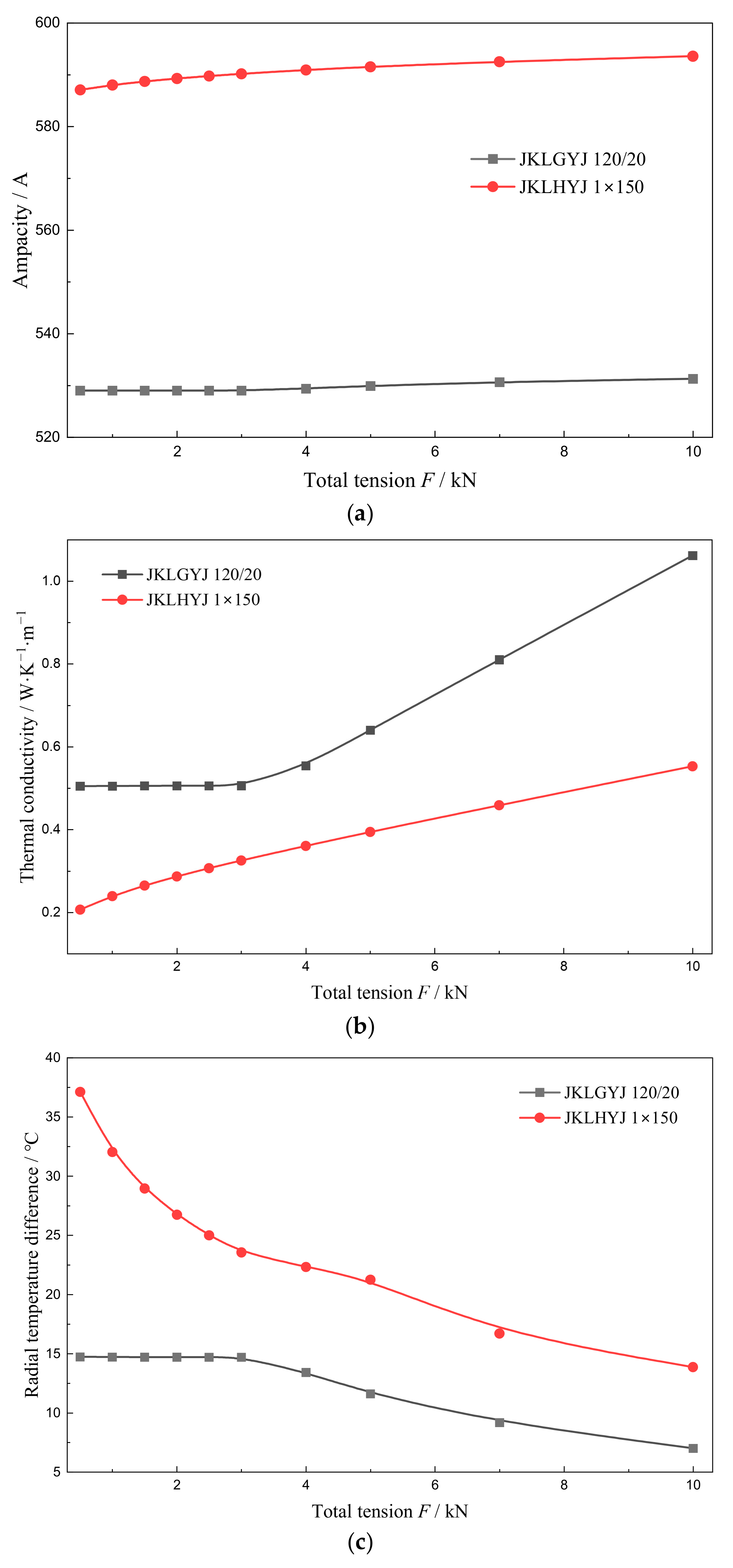
Conductor stress affects radial heat transfer performance by altering the interlayer contact state. Its influence on the ampacity under average meteorological conditions can better reflect the general patterns in actual operation; therefore, these conditions are selected for analysis. Figure 9 illustrates the influence of conductor stress on the ampacity of, equivalent radial thermal conductivity of, and radial temperature difference in the two types of compacted conductor overhead insulated cables under these meteorological conditions.

Figure 9. Comparison of conductor ampacity, equivalent radial thermal conductivity, and radial temperature difference under different tensions. (a) Variation in ampacity with total tension; (b) variation in equivalent radial thermal conductivity with total tension; (c) variation in radial temperature difference with total tension.

It can be seen from Figure 9a that as the conductor stress increases from 0.5 kN to 10 kN, the ampacity of both types of cables shows a slowly increasing trend. The ampacity of JKLGYJ 120/20 increases by 2.3 A; the ampacity of JKLHYJ 150 increases by 6.5 A, indicating that conductor stress has a limited impact on the ampacity. The explanation of this finding is provided in Appendix B.3. Figure 9b shows that with the increasing conductor stress, the equivalent radial thermal conductivity of both types of cables tends to increase. This is because increased tension leads to tighter interlayer contact, increasing the asperity contact area and decreasing the thin-layer air gap thickness, thereby improving radial heat transfer performance, which is consistent with the predictions of the compacted conductor contact model. Figure 9c shows that the radial temperature difference in the conductors decreases with the increasing tension, verifying the physical mechanism by which tension affects contact thermal resistance and thereby alters the temperature distribution.

5.4. Influence of Wind Speed on Conductor Radial Temperature Difference and Ampacity

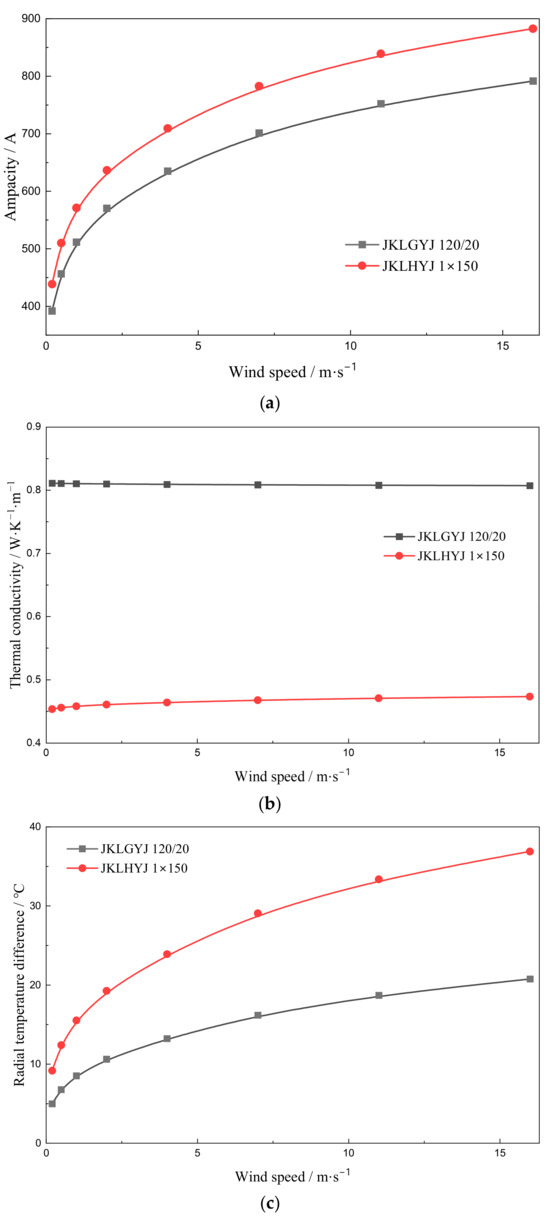
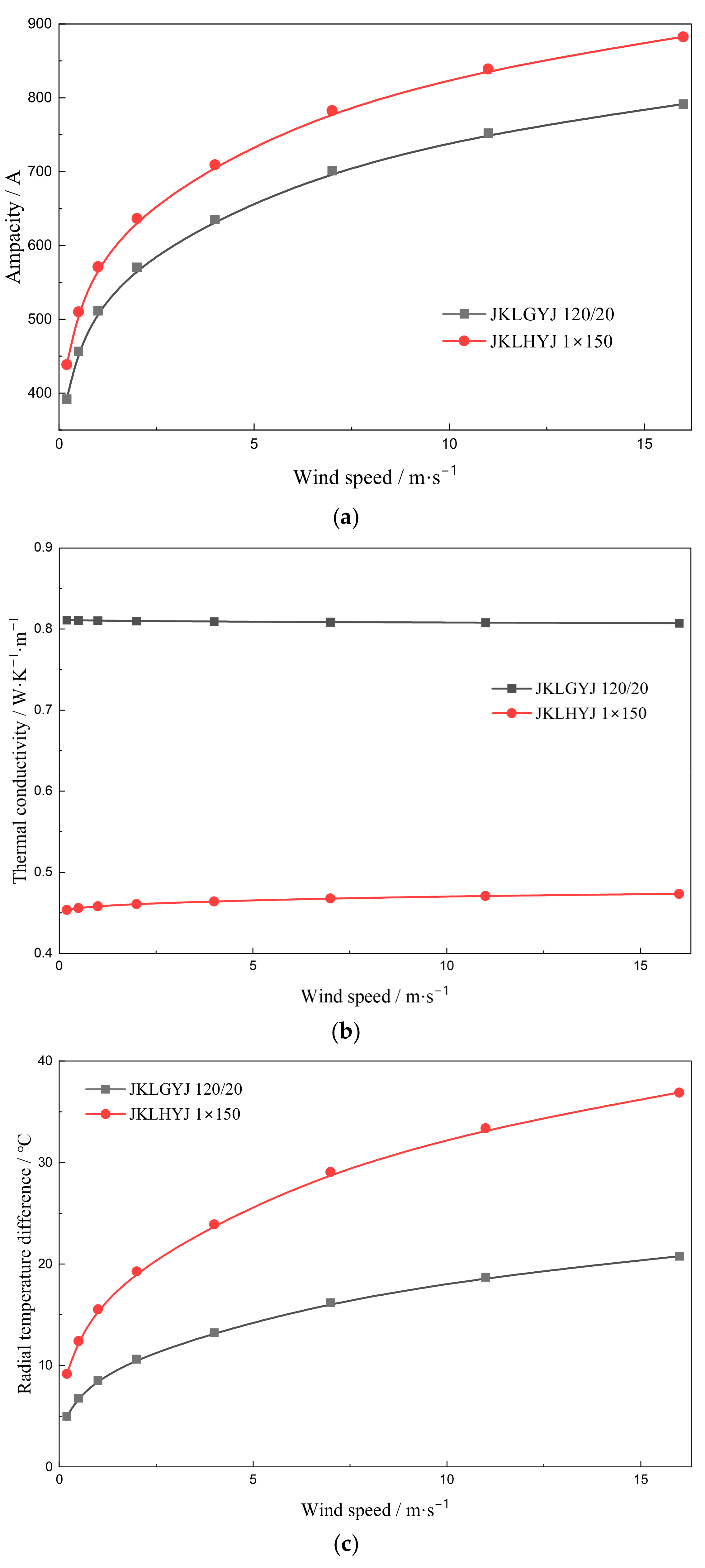
Wind speed is a decisive factor affecting convective heat transfer intensity, and its influence on the ampacity exhibits significant nonlinear characteristics over a wide range of wind speeds. Therefore, high-wind meteorological conditions are selected for analysis. These conditions cover a wide wind speed range from natural convection to strong winds, enabling a comprehensive revelation of the influence patterns of wind speed on thermal behavior. Figure 10 illustrates the influence of wind speed on the ampacity of, equivalent radial thermal conductivity of, and radial temperature difference in the two types of overhead insulated cables under these conditions.

Figure 10. Comparison of equivalent radial thermal conductivity, radial temperature difference, and ampacity under different wind speeds. (a) Variation in ampacity with wind speed; (b) variation in equivalent radial thermal conductivity with wind speed; (c) variation in radial temperature difference with wind speed.

As the wind speed increases, convective heat transfer intensifies, and the ampacity of both types of cables shows an increasing trend, as shown in Figure 10a. Notably, the variation in the ampacity with wind speed exhibits significant nonlinear characteristics: at low wind speeds (0–5 m/s), the ampacity increases rapidly with the increasing wind speed, indicating that the enhancement effect of convective heat transfer is most significant in the low wind speed range; as the wind speed continues to increase, the increase in the ampacity gradually slows down, reflecting the physical law that convective heat transfer tends to saturate.

Figure 10b shows that changes in wind speed have essentially no effect on the equivalent radial thermal conductivity of the two types of cables, further confirming that the radial heat transfer performance of the conductor depends only on its own structure and is independent of the ambient wind speed. Combined with the analysis in Figure 8b and Figure 10b, it can be understood that the equivalent radial thermal conductivity is an intrinsic property of the conductor and is not affected by external thermal boundary conditions.

It can be seen from Figure 10c that as the wind speed increases, the radial temperature difference in the conductors gradually increases. With the radial thermal conductivity of the conductor remaining essentially unchanged, according to the thermal circuit model, the radial temperature difference in the conductor is proportional to the ampacity. Therefore, the increase in the ampacity brought about by the increased wind speed inevitably leads to an increase in the radial temperature difference, which is determined by the coupling mechanism between internal heat conduction within the conductor and external convective heat transfer.

6. Conclusions

This paper has proposed an ampacity calculation method for overhead insulated cables with compacted conductors, accounting for their “plastic-then-elastic” deformation characteristics. The main conclusions are as follows:

(1)

A radial heat transfer model for compacted conductors is established by incorporating material plastic flow and elastic substrate deformation into the formulations for interlayer thermal contact conductance and thin-layer air gap thickness, with the air void equivalent distance corrected by the fill factor. Wind tunnel tests on JKLGYJ 240/30 cables validate the model, yielding a radial temperature difference of 2.41 °C against the measured 2.6 °C, significantly outperforming the conventional Morgan model.

(2)

Aluminum alloy core cables (JKLHYJ 150) exhibit higher ampacity than steel-reinforced aluminum cables (JKLGYJ 120/20) with comparable cross-sectional areas.

(3)

The equivalent radial thermal conductivity of compacted conductors is independent of environmental factors. Increasing the conductor tension enhances the thermal conductivity but has a negligible effect on the ampacity (variation < 0.1%).

(4)

Wind speed affects the ampacity with distinct nonlinear characteristics: the ampacity increases rapidly in the low wind speed range (0–5 m/s) but exhibits diminishing returns beyond 10 m/s as convective heat transfer approaches saturation.

Despite its contributions, the proposed ampacity calculation method has several limitations. Firstly, the model describes the contact surfaces with Gaussian distribution of the asperity’s height and random distribution of the slope, which may not fully reflect real-world conditions; secondly, the approximate formula for evaluating the fraction of actual area in contact is constrained by the parameter range of ${\mathsf{\delta }}_{\mathrm{g}}/{\mathsf{\sigma }}_{\mathrm{m}}$ from 1.0 to 3.0, which may not hold true in all practical scenarios. These limitations suggest that our conclusions should be interpreted with caution. Future research should focus on extending the model’s validation to diverse conductor types, directly measuring interlayer temperatures to obtain the full current–temperature characteristics, and developing a transient analysis capability for dynamic rating applications.

Appendix A.1

The parameters of the conductor material used in this paper are shown in the following Table A1, Table A2 and Table A3.

Table A1. The electro-thermal parameters of the conductor material.

Material	${\mathsf{\rho }}_{20}$ Stranded nΩ·m	${\mathsf{\rho }}_{20}$ Compacted * nΩ·m	${\mathsf{\alpha }}_{20}$ 1/K	${\mathsf{\zeta }}_{20}$ 1/K2	${\mathsf{\mu }}_{\mathit{r}}$
Aluminum	28.2639	28.4975	0.00403	8.0 × 10−7	1.00002
Steel	191.5667	/	0.00455	6.0 × 10−6	400
Aluminum alloy	28.9765	29.2220	0.00400	8.0 × 10−7	1.00003

* The filling factor of the compacted conductor is 0.84.

Table A1. The electro-thermal parameters of the conductor material.

Material	${\mathsf{\rho }}_{20}$ Stranded nΩ·m	${\mathsf{\rho }}_{20}$ Compacted * nΩ·m	${\mathsf{\alpha }}_{20}$ 1/K	${\mathsf{\zeta }}_{20}$ 1/K2	${\mathsf{\mu }}_{\mathit{r}}$
Aluminum	28.2639	28.4975	0.00403	8.0 × 10−7	1.00002
Steel	191.5667	/	0.00455	6.0 × 10−6	400
Aluminum alloy	28.9765	29.2220	0.00400	8.0 × 10−7	1.00003

* The filling factor of the compacted conductor is 0.84.

Table A2. The mechanical parameters of the conductor material.

Material	$\mathit{E}$ GPa	$\mathit{\beta }$ 1/K	$\mathit{H}$ GPa	$\mathit{v}$
Aluminum	59	23.0 × 10−6	0.48	0.33
Steel	196	11.5 × 10−6	1.59	0.26
Aluminum alloy	63	23.0 × 10−6	0.84	0.33

Table A2. The mechanical parameters of the conductor material.

Material	$\mathit{E}$ GPa	$\mathit{\beta }$ 1/K	$\mathit{H}$ GPa	$\mathit{v}$
Aluminum	59	23.0 × 10−6	0.48	0.33
Steel	196	11.5 × 10−6	1.59	0.26
Aluminum alloy	63	23.0 × 10−6	0.84	0.33

Table A3. The surface parameters of the conductor material.

Material	$\mathbf{tan}{\mathit{\theta }}_{\mathbf{m}}$ Stranded	${\mathsf{\sigma }}_{\mathbf{m}}$ Stranded μm	$\mathbf{tan}{\mathit{\theta }}_{\mathbf{m}}$ Compacted	${\mathsf{\sigma }}_{\mathbf{m}}$ Compacted μm
Aluminum	0.05	1	0.04	0.679
Steel	0.1	3	/	/
Aluminum alloy	0.075	2	0.065	1.471

Table A3. The surface parameters of the conductor material.

Material	$\mathbf{tan}{\mathit{\theta }}_{\mathbf{m}}$ Stranded	${\mathsf{\sigma }}_{\mathbf{m}}$ Stranded μm	$\mathbf{tan}{\mathit{\theta }}_{\mathbf{m}}$ Compacted	${\mathsf{\sigma }}_{\mathbf{m}}$ Compacted μm
Aluminum	0.05	1	0.04	0.679
Steel	0.1	3	/	/
Aluminum alloy	0.075	2	0.065	1.471

Appendix A.2

Appendix A.2.1

According to CIGRE TB 601 [8], the forced convective heat loss $P_{\mathrm{c}}$ is given by

$$P_{\mathrm{c}}=\pi \cdot {\lambda }_{\mathrm{f}}\cdot \left(T_{\mathrm{ins}}-T_{\mathrm{a}}\right)\cdot Nu$$

(A1)

where ${\lambda }_{\mathrm{f}}$ is the thermal conductivity of the air at the film temperature $T_{\mathrm{f}}$.

${\lambda }_{\mathrm{f}}$ and $T_{\mathrm{f}}$ can be calculated according to

$$\begin{array}{l}{\lambda }_{\mathrm{f}}=0.02368+7.23\times {10}^{-5}\cdot T_{\mathrm{f}}-2.763\times {10}^{-8}\cdot T_{\mathrm{f}}^2\\ T_{\mathrm{f}}=0.5\left(T_{\mathrm{ins}}+T_{\mathrm{a}}\right)\end{array}$$

(A2)

The airflow is considered perpendicular to the overhead insulated cable; thus, the Reynolds number $Nu$ can be expressed as

$$Nu=B_1\cdot R{e}^{B_2}$$

(A3)

where $B_1$ and $B_2$ are constants corresponding to the Reynolds number $Re$, and their relationship is shown in Table A4. $Re$ is given by

$$Re={\displaystyle \frac{V_{\mathrm{W}}\cdot D_{\mathrm{ins}}}{v_{\mathrm{f}}}}$$

(A4)

where $V_{\mathrm{W}}$ is the wind speed; $D_{\mathrm{ins}}$ is the diameter of the overhead insulated cable; and $v_{\mathrm{f}}$ is the dynamic viscosity of the air at film temperature $T_{\mathrm{f}}$, which can be calculated as

$$v_{\mathrm{f}}={\displaystyle \frac{\left(17.239+0.04635\cdot T_{\mathrm{f}}-2.03\times {10}^{-5}\cdot T_{\mathrm{f}}^2\right)\times {10}^{-6}}{\frac{1.293-1.525\times {10}^{-4}\cdot y+6.379\times {10}^{-9}\cdot y^2}{1+0.00367\cdot T_{\mathrm{f}}}}}$$

(A5)

Table A4. Relationship among $B_1$, B₂ and R_e for overhead insulated cables with perpendicular air flow.

$\mathbf{R}\mathbf{e}$	${\mathbf{B}}_1$	${\mathbf{B}}_2$
35–5000	0.583	0.471
5000–50,000	0.148	0.633
50,000–200,000	0.0208	0.814

Table A4. Relationship among $B_1$, B₂ and R_e for overhead insulated cables with perpendicular air flow.

$\mathbf{R}\mathbf{e}$	${\mathbf{B}}_1$	${\mathbf{B}}_2$
35–5000	0.583	0.471
5000–50,000	0.148	0.633
50,000–200,000	0.0208	0.814

Appendix A.2.2

According to CIGRE TB 601, the radiated heat loss $P_{\mathrm{r}}$ is given by

$$P_{\mathrm{r}}=\pi \cdot D_{\mathrm{ins}}\cdot {\sigma }_{\mathrm{B}}\cdot {\epsilon }_{\mathrm{S}}\cdot \left[{\left(T_{\mathrm{ins}}+273.15\right)}^4-{\left(T_{\mathrm{a}}+273.15\right)}^4\right]$$

(A6)

where ${\sigma }_{\mathrm{B}}$ is the Stefan–Boltzmann constant; ${\epsilon }_{\mathrm{S}}$ is the emissivity of the insulating surface. Here, ${\epsilon }_{\mathrm{S}}=0.8$.

Appendix A.2.3

According to CIGRE TB 601, the solar gain $P_{\mathrm{S}}$ is given by

$$P_{\mathrm{S}}={\alpha }_{\mathrm{S}}\cdot D_{\mathrm{ins}}\cdot \left[I_{\mathrm{B}}\left(y\right)\cdot \left(\sin \left(\eta \right)+{\displaystyle \frac{\pi }{2}}\cdot F_{\mathrm{R}}\cdot \sin \left(H_{\mathrm{S}}\right)\right)+I_{\mathrm{d}}\cdot \left(1+{\displaystyle \frac{\pi }{2}}\cdot F\right)\right]$$

(A7)

where ${\alpha }_{\mathrm{S}}$ is the absorptivity of the cable surface; $I_{\mathrm{B}}\left(y\right)$ is the direct solar radiation at an altitude of $y$; $I_{\mathrm{d}}$ is the diffuse radiation; $\eta$ is the angle of the solar beam with respect to the axis of the conductor; and ${\mathrm{F}}_{\mathrm{R}}$ is the reflectance of the ground. In this paper, we set ${\alpha }_{\mathrm{S}}=0.8$ and $F_{\mathrm{R}}=0.15$.

The direct solar radiation $I_{\mathrm{B}}\left(y\right)$ can be calculated by the following equations:

$$\begin{array}{l}{I}_{\mathrm{B}}\left(y\right)=I_{\mathrm{B}}\left(0\right)\left[1+0.00014\cdot y\cdot \left({\displaystyle \frac{1367}{I_{\mathrm{B}}\left(0\right)}}-1\right)\right]\\ I_{\mathrm{B}}\left(0\right)=N_{\mathrm{S}}\cdot {\displaystyle \frac{1280·\sin \left(H_{\mathrm{S}}\right)}{\sin \left(H_{\mathrm{S}}\right)+0.314}}\\ H_{\mathrm{S}}=\arcsin \left(\sin \phi \cdot \sin {\delta }_{\mathrm{S}}+\cos \phi \cdot \cos {\delta }_{\mathrm{S}}\cdot \cos Z\right)\end{array}$$

(A8)

where $N_{\mathrm{S}}$ is a clearness ratio, $\phi$ is the latitude, ${\delta }_{\mathrm{S}}$ is the solar declination, and $Z$ is the solar azimuth. The values of parameters $N_{\mathrm{S}}$, $\phi$, ${\delta }_{\mathrm{S}}$ and $Z$ are summarized in Table 2 in the main text.

The diffuse radiation $I_{\mathrm{d}}$ can be calculated by the following equations:

$$\begin{array}{l}{I}_{\mathrm{d}}=\left(430.5-0.3288\cdot I_{\mathrm{B}}\left(y\right)\right)\cdot \sin \left(H_{\mathrm{S}}\right)\\ \eta =\arccos \left[\cos \left(H_{\mathrm{S}}\right)\cdot \cos \left({\gamma }_{\mathrm{S}}-{\gamma }_{\mathrm{C}}\right)\right]\\ {\gamma }_{\mathrm{S}}=\arcsin \left[{\displaystyle \frac{\cos \left({\delta }_{\mathrm{S}}\right)\sin \left(Z\right)}{\cos \left(H_{\mathrm{S}}\right)}}\right]\end{array}$$

(A9)

where ${\gamma }_{\mathrm{C}}$ is the azimuth of the conductor; ${\mathsf{\gamma }}_{\mathrm{S}}$ is the azimuth of the sun.

Appendix A.2.4

According to IEC 60287-1-1 [17], the dielectric loss $P_{\mathrm{d}}$ is given by

$$P_{\mathrm{d}}=2\pi f\cdot {\displaystyle \frac{2\pi {\epsilon }_0{\epsilon }_{\mathrm{ins}}}{\ln \left(\frac{D_{\mathrm{ins}}}{D_{\mathrm{sh}}}\right)}}\cdot U_{\mathrm{ins}}^2\cdot \tan {\theta }_{\mathrm{ins}}$$

(A10)

where $D_{\mathrm{sh}}$ is the diameter of the conductor screen; ${\mathsf{\epsilon }}_0$ is the permittivity of the vacuum; ${\mathsf{\epsilon }}_{\mathrm{ins}}$ is the relative permittivity of the insulation; $U_{\mathrm{ins}}$ is the voltage applied across the insulation layer; and $\tan { \theta }_{\mathrm{ins}}$ is the loss factor of the insulation.

It should be noted that for 10 kV overhead insulated cables, the dielectric loss is so small that it can be generally neglected. For the JKLHYJ 1 × 150 cable (with parameters $U_0=\mathrm{10,000}/\sqrt{3}\mathrm{V}$, ${\mathsf{\epsilon }}_{\mathrm{ins}}=3.0$, $\tan {\theta }_{\mathrm{ins}}=0.005$ and $U_{\mathrm{ins}}=89 \mathrm{V}$ at a cable height of 10 m above ground), the dielectric loss $P_{\mathrm{d}}$ is 6 × 10⁻⁶ W/m, which is negligible compared to the Joule loss in the conductor ($P_{\mathrm{J}}=9.615 \mathrm{W}/\mathrm{m}$) under 100% load conditions (① + ⑥ + ⑦ in Table 2 in the main text).

Appendix A.3

The content of this section mainly refers to Reference [20] in the main text.

When a load is applied to an asperity, the total displacement $\mathsf{\Delta }C$ including the plastic deformation of the asperity’s top and elastic deformation of the substrate can be written as

$$\Delta C={\displaystyle \frac{1}{2r_i}}{a}_i^2+{\displaystyle \frac{\pi H}{2E^{\prime }}}{a}_i={\sigma }_{\mathrm{m}}\left(\xi -{\displaystyle \frac{{\delta }_{\mathrm{g}}}{{\sigma }_{\mathrm{m}}}}\right)$$

(A11)

where $a_i$ is the radius of a contact point; $r_i$ is the radius of curvature of an asperity; and $\xi$ is the dimensionless distance when the asperity first came in contact.

Solve for $a_i$ from Equation (A11) and then make it dimensionless ($\overline{a_i}$) according to Equation (A12).

$$\begin{array}{l}{\overline{a}}_i={\left({\displaystyle \frac{{\pi }^2}{4}}{r}_i^2{\gamma }_i^2+2{\overline{r}}_i\left(\xi -{\displaystyle \frac{{\delta }_{\mathrm{g}}}{{\sigma }_{\mathrm{m}}}}\right)\right)}^{{\displaystyle \frac{1}{2}}}-{\displaystyle \frac{\pi }{2}}{\overline{r}}_i{\gamma }_i\\ {\overline{a}}_i=a_i{\displaystyle \frac{\tan {\theta }_{\mathrm{m}}}{{\sigma }_{\mathrm{m}}}}\\ {\overline{r}}_i=r_i{\displaystyle \frac{{\tan }^2{\theta }_{\mathrm{m}}}{{\sigma }_{\mathrm{m}}}}\\ {\gamma }_i={\displaystyle \frac{H}{E^{\prime }\tan {\theta }_{\mathrm{m}}}}\end{array}$$

(A12)

The definition of $A_{\mathrm{r}}/A_{\mathrm{a}}$ is

$$\begin{array}{cc}\hfill {\displaystyle \frac{A_{\mathrm{r}}}{A_{\mathrm{a}}}}& ={\displaystyle {\int }_{\frac{{\delta }_{\mathrm{g}}}{{\sigma }_{\mathrm{m}}}}^{\infty }\pi {\overline{a}}_i^2}\overline{{\tau }_i^{\prime }}\mathrm{d}\xi \hfill \\ \hfill & ={\displaystyle {\int }_{\frac{{\delta }_{\mathrm{g}}}{{\sigma }_{\mathrm{m}}}}^{\infty }2\pi \left(\xi -\frac{{\delta }_{\mathrm{g}}}{{\sigma }_{\mathrm{m}}}\right)}{\overline{r}}_i\overline{{\tau }_i^{\prime }}\mathrm{d}\xi -{\pi }^2{\gamma }_i{\displaystyle {\int }_{\frac{{\delta }_{\mathrm{g}}}{{\sigma }_{\mathrm{m}}}}^{\infty }{\overline{a}}_i{\overline{r}}_i}\overline{{\tau }_i^{\prime }}\mathrm{d}\xi \hfill \\ \hfill & ={\displaystyle \frac{A_{\mathrm{r}}}{A_{\mathrm{a}}}}{|}_{\mathrm{pure}}-{\pi }^2{\gamma }_i{\displaystyle {\int }_{\frac{{\delta }_{\mathrm{g}}}{{\sigma }_{\mathrm{m}}}}^{\infty }{\overline{a}}_i{\overline{r}}_i}\overline{{\tau }_i^{\prime }}\mathrm{d}\xi \hfill \end{array}$$

(A13)

where ${\mathsf{\tau }}_i$ is the number of contacts per unit area and $\overline{{\mathsf{\tau }}_i}=\left({\mathsf{\tau }}_i{\mathsf{\sigma }}_m^2\right)/\left({\tan }^2\mathsf{\theta }\right)$;

Substituting $\overline{r_i}\cdot \overline{{\mathsf{\tau }}_i^{\prime }}=\mathsf{\xi }\cdot \exp \left(-{\mathsf{\xi }}^2/2\right)/{\left(2\mathsf{\pi }\right)}^{3/2}$ and $\overline{r_i}=4/\left({\pi }^{3/2}\cdot \xi \right)$ into Equation (A13) yields

$$\begin{array}{l}{\displaystyle \raisebox{1ex}{$\left(A_{\mathrm{r}}/A_{\mathrm{a}}\right)$}\!\left/ \!\raisebox{-1ex}{$\left(A_{\mathrm{r}}/A_{\mathrm{a}}\right){|}_{\mathrm{pure}}$}\right.}=1-\\ {\displaystyle \frac{{\displaystyle {\int }_{\frac{{\delta }_{\mathrm{g}}}{{\sigma }_{\mathrm{m}}}}^{\infty }\left[{\left(\frac{{\pi }^2{\gamma }_i^2}{4}{\left(\frac{4{\sigma }_{\mathrm{m}}}{{\pi }^{3/2}\xi {\tan }^2{\theta }_{\mathrm{m}}}\right)}^2+\frac{8}{{\pi }^{3/2}\xi }\left(\xi -\frac{{\delta }_{\mathrm{g}}}{{\sigma }_{\mathrm{m}}}\right)\right)}^{\frac{1}{2}}-\frac{2{\gamma }_i}{{\pi }^{1/2}\xi }\right]}\frac{\xi \cdot \exp \left(-\frac{{\xi }^2}{2}\right)}{{\left(32\pi \right)}^{1/2}}\mathrm{d}\xi }{\frac{p_{\mathrm{q}}}{H+p_{\mathrm{q}}}}}\end{array}$$

(A14)

Equation (A14) is solved by numerical methods under the boundary conditions ${\mathsf{\delta }}_{\mathrm{g}}/{\mathsf{\sigma }}_{\mathrm{m}}=1.0$ to ${\mathsf{\delta }}_{\mathrm{g}}/{\mathsf{\sigma }}_{\mathrm{m}}=3.0$,

$${\displaystyle \raisebox{1ex}{$\left(A_{\mathrm{r}}/A_{\mathrm{a}}\right)$}\!\left/ \!\raisebox{-1ex}{$\left(A_{\mathrm{r}}/A_{\mathrm{a}}\right){|}_{\mathrm{pure}}$}\right.}={\displaystyle \frac{1}{1+2.5{\left(H/\left(E^{\prime }\tan {\theta }_{\mathrm{m}}\right)\right)}^{1.2}}}$$

(A15)

Based on Equation (A15), the mathematical expression of Equation (6) in the main text can be directly derived. It should be noted that Equation (6) holds true when the parameter ${\delta }_{\mathrm{g}}/{\sigma }_{\mathrm{m}}$ ranges from 1.0 to 3.0, which covers the vast majority of practical cases.

Appendix B.1

Table A5 provides additional information corresponding to the case shown in Figure 6: temperatures at the same location on an identical compacted conductor were obtained through experimental measurement, simulation of the Morgan model, and simulation of the modified model, respectively. We found that the radial temperature distributions from the three methods follow a similar trend: the temperature difference across the conductor increases radially from the inner layer to the outer layer.

It should be noted that securing a temperature sensor (thermocouple) to a given conductor layer requires damaging the outer insulation, the conductor shielding, and the stranded wire structure around the measurement point. Therefore, during testing, care should be taken to restore the surrounding conditions at the measurement location. The installation of the thermocouple may affect the accuracy of the temperature measurement. In the main text of this paper, the temperature difference between the innermost and outermost conductors is used to characterize the thermal state, which also helps mitigate measurement errors introduced by sensor installation.

Table A5. Comparison of experimental and calculated temperatures for conductors at different layers for JKLGYJ 240/30.

Method	${\mathit{T}}_{\mathbf{c}0}$/°C	${\mathit{T}}_{\mathbf{c}1}$/°C	${\mathit{T}}_{\mathbf{c}2}$/°C	${\mathit{T}}_{\mathbf{c}3}$/°C
Experimental measurement	52.8	52.8	52.1	50.2
Morgan model	50.87	50.82	50.62	48.62
Modified model	51.03	50.98	50.76	48.62

Table A5. Comparison of experimental and calculated temperatures for conductors at different layers for JKLGYJ 240/30.

Method	${\mathit{T}}_{\mathbf{c}0}$/°C	${\mathit{T}}_{\mathbf{c}1}$/°C	${\mathit{T}}_{\mathbf{c}2}$/°C	${\mathit{T}}_{\mathbf{c}3}$/°C
Experimental measurement	52.8	52.8	52.1	50.2
Morgan model	50.87	50.82	50.62	48.62
Modified model	51.03	50.98	50.76	48.62

Appendix B.2

The structure of JKLHYJ 1 × 150 is more sparse than JKLGYJ 120/20, resulting in a higher interlayer contact thermal resistance in Figure 8b in the main text. Table A6 and Table A7 show the heat transfer coefficients between layers for JKLGYJ 120/20 and JKLHYJ 1 × 150, respectively.

For the JKLGYJ 120/20 conductor, since the tensile load is almost entirely sustained by the steel core, the aluminum strands bear no mechanical stress. Thus, the radial stress in the aluminum strands is zero, which results in no heat transfer through the aluminum-to-aluminum contact interfaces or aluminum-to-steel contact interface. As indicated in Table A6, the radial heat transfer in the JKLGYJ 120/20 conductor is primarily contributed by the heat conduction through air voids.

For the JKLHYJ 1 × 150 conductor, the data in Table A7 indicate that radial heat propagation is governed by distinct mechanisms between layers. Between layer 0 and layer 1, heat transfer is dominated by conduction through the contact interfaces (characterized by $h_{\mathrm{m}\mathrm{c}\mathrm{o}\mathrm{n}}{A}_{\mathrm{m}}$ and $h_{\mathrm{g}\mathrm{c}\mathrm{o}\mathrm{n}}{A}_{\mathrm{g}}$). In contrast, between layer 1 and layer 2, conduction through air voids becomes the dominant mechanism. However, for the conductor as a whole, radial heat conduction is primarily governed by heat transfer through voids. This is because, within layer 0, only four aluminum alloy wires generate heat, which means just a small portion of the heat is dominated by contact heat transfer.

A comparison of Table A6 and Table A7 shows that JKLGYJ 120/20 has a higher heat transfer coefficient of air voids than JKLHYJ 1 × 150, indicating that JKLHYJ 1 × 150 therefore has a looser structure.

Table A6. The heat transfer coefficients between layers for JKLGYJ 120/20.

JKLGYJ 120/20	${\mathit{h}}_{\mathbf{m}\mathbf{c}\mathbf{o}\mathbf{n}}{\mathit{A}}_{\mathbf{m}}$ W·K−1·m−1	${\mathit{h}}_{\mathbf{g}\mathbf{c}\mathbf{o}\mathbf{n}}{\mathit{A}}_{\mathbf{g}}$ W·K−1·m−1	${\mathit{h}}_{\mathbf{v}\mathbf{c}\mathbf{o}\mathbf{n}}{\mathit{A}}_{\mathbf{v}}$ W·K−1·m−1
Layer 0–1	0.04525	0.1111	1.2354
Layer 1–2	0	0	1.3027
Layer 2–3	0	0	2.8548

Table A6. The heat transfer coefficients between layers for JKLGYJ 120/20.

JKLGYJ 120/20	${\mathit{h}}_{\mathbf{m}\mathbf{c}\mathbf{o}\mathbf{n}}{\mathit{A}}_{\mathbf{m}}$ W·K−1·m−1	${\mathit{h}}_{\mathbf{g}\mathbf{c}\mathbf{o}\mathbf{n}}{\mathit{A}}_{\mathbf{g}}$ W·K−1·m−1	${\mathit{h}}_{\mathbf{v}\mathbf{c}\mathbf{o}\mathbf{n}}{\mathit{A}}_{\mathbf{v}}$ W·K−1·m−1
Layer 0–1	0.04525	0.1111	1.2354
Layer 1–2	0	0	1.3027
Layer 2–3	0	0	2.8548

Table A7. The heat transfer coefficients between layers for JKLHYJ 1 × 150.

JKLGYJ 1 × 150	${\mathit{h}}_{\mathbf{m}\mathbf{c}\mathbf{o}\mathbf{n}}{\mathit{A}}_{\mathbf{m}}$ W·K−1·m−1	${\mathit{h}}_{\mathbf{g}\mathbf{c}\mathbf{o}\mathbf{n}}{\mathit{A}}_{\mathbf{g}}$ W·K−1·m−1	${\mathit{h}}_{\mathbf{v}\mathbf{c}\mathbf{o}\mathbf{n}}{\mathit{A}}_{\mathbf{v}}$ W·K−1·m−1
Layer 0–1	1.5690	0.6491	0.5185
Layer 1–2	0.0892	0.2967	1.6449

Table A7. The heat transfer coefficients between layers for JKLHYJ 1 × 150.

JKLGYJ 1 × 150	${\mathit{h}}_{\mathbf{m}\mathbf{c}\mathbf{o}\mathbf{n}}{\mathit{A}}_{\mathbf{m}}$ W·K−1·m−1	${\mathit{h}}_{\mathbf{g}\mathbf{c}\mathbf{o}\mathbf{n}}{\mathit{A}}_{\mathbf{g}}$ W·K−1·m−1	${\mathit{h}}_{\mathbf{v}\mathbf{c}\mathbf{o}\mathbf{n}}{\mathit{A}}_{\mathbf{v}}$ W·K−1·m−1
Layer 0–1	1.5690	0.6491	0.5185
Layer 1–2	0.0892	0.2967	1.6449

Appendix B.3

In this section, we attempt to explain the computational results shown in Figure 9 in the main text—namely, why changes in radial thermal conductivity do not affect the ampacity from the perspective of thermal balance.

As shown in Table A8, we calculated $P_{\mathrm{J}}$, $P_{\mathrm{S}}$, $P_{\mathrm{c}}$, and $P_{\mathrm{r}}$ under different tensions and found that although varying the tension can significantly alter the equivalent radial thermal conductivity of the conductor, the system always converges to the same thermal equilibrium state. Therefore, the Joule loss of the conductor and the temperature of the outermost conductor remain constant.

Different equivalent radial thermal conductivities do make the temperature redistribution, but this variation does not lead to a notable change in the loss distribution. In fact, for the JKHLYJ 1 × 150 cable studied in this paper, the temperature of the outermost 16 aluminum alloy strands remains unchanged; only the inner 10 aluminum alloy strands participate in the redistribution of temperature and losses. It is for this reason that the ampacity turns out to be insensitive to variations in radial thermal conductivity.

Table A8. Thermal equilibrium at different values of total tension for JKLHYJ 1 × 150.

Total Tension/kN	${\mathit{P}}_{\mathbf{J}}$/W·m−1	${\mathit{P}}_{\mathbf{S}}$/W·m−1	${\mathit{P}}_{\mathbf{c}}$/W·m−1	${\mathit{P}}_{\mathbf{r}}$
2	96.26	25.54	99.66	22.17
4	96.26	25.54	99.66	22.17
6	96.26	25.54	99.66	22.17
8	96.26	25.54	99.66	22.17
10	96.26	25.54	99.66	22.17

Table A8. Thermal equilibrium at different values of total tension for JKLHYJ 1 × 150.

Total Tension/kN	${\mathit{P}}_{\mathbf{J}}$/W·m−1	${\mathit{P}}_{\mathbf{S}}$/W·m−1	${\mathit{P}}_{\mathbf{c}}$/W·m−1	${\mathit{P}}_{\mathbf{r}}$
2	96.26	25.54	99.66	22.17
4	96.26	25.54	99.66	22.17
6	96.26	25.54	99.66	22.17
8	96.26	25.54	99.66	22.17
10	96.26	25.54	99.66	22.17

References

- Soares, C.G.; Taralli, C.; Bonfa, A.R. Insulated Overhead Lines. IEEE Trans. Power Appar. Syst. 1982, PAS-101, 2273–2277. [Google Scholar] [CrossRef] [Scilit]
- Wang, Q.; Liu, G.; Fang, B.; Liu, Z.; Wang, Y.; Su, J. Analysis of Causes for Overhead Insulated Wires Breakage. In Proceedings of the 2018 China International Conference on Electricity Distribution (CICED), Tianjin, China, 17–19 September 2018; pp. 1279–1283. [Google Scholar]
- National Energy Administration; China Electricity Council. 2024 National Electric Power Reliability Annual Report; National Energy Administration, China Electricity Council: Beijing, China, 2025. [Google Scholar]
- Luejai, W.; Suwanasri, T.; Suwanasri, C. Condition Assessment of Overhead Transmission Line Using Weighting and Scoring Method and IT Application. J. Electr. Eng. Technol. 2021, 16, 2981–2993. [Google Scholar] [CrossRef] [Scilit]
- Enescu, D.; Russo, A.; Porumb, R.; Seritan, G. Dynamic Thermal Rating of Electric Cables: A Conceptual Overview. In Proceedings of the 2020 55th International Universities Power Engineering Conference (UPEC), Turin, Italy, 1–4 September 2020; pp. 1–6. [Google Scholar]
- Zhang, Y.; Sun, H.; Zhang, X.; Chen, Z.; Zhou, L.; Huang, X. Economic Analysis of Aluminium Conductor Composite Core and Conventional Aluminium Conductor Steel Reinforced Conductors in Overhead Ultra-High Voltage Transmission Lines. IET Gener. Transm. Distrib. 2023, 17, 1098–1110. [Google Scholar] [CrossRef] [Scilit]
- CIGRE Working Group 22.12. Thermal Behaviour of Overhead Conductors: Technical Brochures 207; CIGRE: Paris, France, 2002. [Google Scholar]
- CIGRE Working Group B2.42. Guide for Thermal Rating Calculations of Overhead Lines: Technical Brochure 601; CIGRE: Paris, France, 2014. [Google Scholar]
- IEEE Std 738-2023; IEEE Standard for Calculating the Current-Temperature of Bare Overhead Conductors. IEEE Power & Energy Society: Piscataway, NJ, USA, 2023.
- Castro, P.; Arroyo, A.; Martinez, R.; Manana, M.; Domingo, R.; Laso, A.; Lecuna, R. Study of Different Mathematical Approaches in Determining the Dynamic Rating of Overhead Power Lines and a Comparison with Real Time Monitoring Data. Appl. Therm. Eng. 2017, 111, 95–102. [Google Scholar] [CrossRef] [Scilit]
- Zia, Z.; Kumru, C.F. Numerical Assessment of Thermal Effects in Bundled Overhead Conductors for Dynamic Line Rating. Appl. Sci. 2025, 15, 10210. [Google Scholar] [CrossRef] [Scilit]
- Morgan, V.T. The Radial Temperature Distribution and Effective Radial Thermal Conductivity in Bare Solid and Stranded Conductors. IEEE Trans. Power Deliv. 1990, 5, 1443–1452. [Google Scholar] [CrossRef] [Scilit]
- Dong, X.C.; Qu, F.R.; Li, Y.F.; Fang, B.L.; Wang, Y.Q.; Li, S.; Liu, G. Construction of thermal conduction model for overhead conductor ampacity-temperature distribution under convection conditions. Adv. Technol. Electr. Eng. Energy 2019, 38, 54–60. [Google Scholar]
- Minambres, J.F.; Barandiaran, J.J.; Alvarez-Isasi, R.; Zorrozua, M.A.; Zamora, I.; Mazon, A.J. Radial Temperature Distribution in ACSR Conductors Applying Finite Elements. IEEE Trans. Power Deliv. 1999, 14, 472–480. [Google Scholar] [CrossRef] [Scilit]
- Wang, F.; Song, C.; Chen, X.; Liu, Z. Radial Temperature Distribution Characteristics of Long-Span Transmission Lines Under Forced Convection Conditions. Processes 2025, 13, 2273. [Google Scholar] [CrossRef] [Scilit]
- Yu, J.; Wu, C.; Huang, H.; Xie, D.; Qin, F.; Jiang, J.; He, G. Discussion on AC Resistance and Temperature of ACSR Based on Finite Element Model Assistance. Energies 2025, 18, 539. [Google Scholar] [CrossRef] [Scilit]
- 60287-1-1-2023; Calculation of the Current Rating—Part 1-1: Current Rating Equations(100% Load Factor) and Calculation of Losses-General. IEC: Geneva, Switzerland, 2023.
- Morgan, V.T. The Thermal Rating of Overhead-Line Conductors Part I. The Steady-State Thermal Model. Electr. Power Syst. Res. 1982, 5, 119–139. [Google Scholar] [CrossRef] [Scilit]
- Pullen, J.; Williamson, J.B. On the Plastic Contact of Rough Surfaces. Proc. R. Soc. Lond. A Math. Phys. Sci. 1972, 327, 159–173. [Google Scholar] [CrossRef] [Scilit]
- Mikić, B.B. Thermal contact conductance; theoretical considerations. Int. J. Heat Mass Transf. 1974, 17, 205–214. [Google Scholar] [CrossRef] [Scilit]
- GB/T 1179-2017; Round wire concentric lay overhead electrical stranded conductors. China Electrical Equipment Industrial Association: Beijing, China, 2017.
- GB/T 14049-2008; Aerial insulated cables for rated voltage of 10 kV. China Electrical Equipment Industrial Association: Beijing, China, 2008.
- State Grid Corporation of China. Typical Design for Distribution Network Engineering: 10 kV Overhead Lines Volume; State Grid Corporation of China: Beijing, China, 2024. [Google Scholar]
Disclaimer/Publisher’s Note: The statements, opinions and data contained in all publications are solely those of the individual author(s) and contributor(s) and not of MDPI and/or the editor(s). MDPI and/or the editor(s) disclaim responsibility for any injury to people or property resulting from any ideas, methods, instructions or products referred to in the content. |
© 2026 by the authors. Licensee MDPI, Basel, Switzerland. This article is an open access article distributed under the terms and conditions of the Creative Commons Attribution (CC BY) license.