


Abstract
In future active distribution networks with high penetrations of renewable energy, flexible loads are expected to play an increasingly important role as reserve resources to support the sustainable and reliable operation of power grids. Accurate evaluation of flexible load reserve capacity is therefore essential for reliable reserve scheduling. Existing research mainly focuses on the operational characteristics and physical constraints of flexible loads, while insufficiently accounting for user response willingness and the uncertainty of user decision-making behavior, which may lead to biased reserve capacity assessments and impair the sustainability of reserve supply in actual grid operation. To address this issue, this paper proposes a results-oriented reserve capacity evaluation method for flexible loads that explicitly incorporates user response willingness. Specifically, a fuzzy logic system is developed to quantitatively characterize the response willingness of electric vehicle (EV) and air-conditioning (AC) users under multiple influencing factors. Then, a probabilistic modeling approach for user decision-making behavior is established using the theory of planned behavior, enabling explicit representation of behavioral uncertainty. Furthermore, a comprehensive reserve capacity evaluation framework for flexible loads is constructed by integrating user willingness states, sustainable response duration, and operational power constraints. Finally, the case studies demonstrate that the proposed method can effectively improve the objectivity of flexible load reserve capacity assessments while maintaining high user participation willingness, thus supporting the long-term sustainable application of flexible loads as grid reserve resources.
1. Introduction
With the accelerating transition toward low-carbon electricity systems, wind power and photovoltaics (PV) are being integrated into active distribution networks at an unprecedented rate [1]. While this transition is essential for decarbonization, it also increases the short-term variability, uncertainty, and ramping requirements that system operators must manage in real time [2]. When reserve resources are insufficient or not sufficiently reliable, renewable curtailment, power imbalances, and operational-security risks may arise [3]. In this context, flexible demand-side resources are increasingly viewed as a valuable complement to conventional reserve providers in renewable-rich distribution systems [4]. Among them, electric vehicles (EVs) are especially promising because of their rapid electrochemical response, growing market penetration, and bidirectional interaction capability [5,6,7]. Existing review studies have highlighted both the technical potential and the broader sociotechnical implications of vehicle-to-grid (V2G) integration [8,9,10].
Most existing studies on EV-based reserve provision have focused on aggregation models, smart charging/discharging strategies, and reserve-oriented dispatch under physical operating constraints [11,12]. More recent studies have introduced incentive mechanisms to enhance the economic attractiveness of EV participation [13,14]. Related work has also considered user willingness, decentralized charging management, and credible reserve capacity quantification for EV aggregators [15,16,17], while other studies have examined willingness-aware dispatch and long-timescale psychological effects in V2G scheduling [18,19]. For air-conditioning (AC) loads, existing research has developed refined load models and equivalent thermal-parameter representations [20,21], investigated energy-reserve market participation and sequential reserve dispatch [22,23], and further explored hierarchical allocation and frequency-support strategies [24,25,26]. Nevertheless, this body of work remains largely device-centered and operation-oriented. In particular, user willingness is still rarely incorporated explicitly into reserve capacity assessment for either EVs or AC loads.
Attention has recently begun to shift toward the behavioral dimension of flexible-load participation. Several studies have explored multi-agent willingness characterization and incentive–willingness–decision frameworks to improve the credibility of EV flexibility or V2G capability assessment [27,28]. Other studies have considered user decision uncertainty in EV charging-station participation and dispatch problems [29]. These studies represent meaningful progress toward user-centered reserve assessments. However, two limitations remain. First, willingness is often analyzed separately from the sustainable operating conditions—such as admissible battery power or acceptable comfort ranges—that ultimately determine whether reserve provision can be maintained over time. Second, willingness is still frequently treated as a proxy for actual participation probability, thereby conflating subjective preference with objective behavioral realization [28]. In practical reserve operation, this simplification may distort the estimation of available reserve capacity and weaken the credibility of dispatch decisions.
Accordingly, the central gap in the existing literature is not merely the absence of another willingness metric, but the lack of an integrated framework that can simultaneously: (1) quantify user willingness for heterogeneous flexible loads under multiple influencing factors; (2) distinguish willingness from realized participation probability; and (3) propagate both willingness states and behavioral uncertainty into reserve capacity evaluation and reserve scheduling while respecting sustainable response duration and operating-power constraints. This gap is of direct practical significance. Reserve capacity may be overestimated when willingness is implicitly interpreted as guaranteed participation, or underestimated when the behavioral influence on feasible operating power is ignored. In either case, the resulting reserve allocation may become insufficient, redundant, or operationally unreliable, thereby undermining the long-term sustainability of flexible-load reserve provision.
To address this issue, this paper combines fuzzy logic with the Theory of Planned Behavior (TPB). Fuzzy logic is adopted because willingness formation is shaped by multiple heterogeneous and partly qualitative factors, whereas large-scale labeled behavioral data are typically unavailable. Under such conditions, a fuzzy-logic framework offers both interpretability and practical implementability for willingness quantification. TPB is introduced because it provides an interpretable behavioral framework for translating willingness-related attitudes into participation probabilities by explicitly accounting for attitude, subjective norms, and perceived behavioral control [30]. In this way, willingness formation and behavior realization are modeled as related but distinct stages, which is more consistent with the actual decision process of flexible load users than direct probability approximation or threshold-based simplification.
On this basis, the main contributions of this paper are summarized as follows:
(1) A unified willingness-quantification framework is developed for EV and AC users by means of a fuzzy logic system. Unlike conventional reserve models that only consider physical operating constraints, the proposed method identifies the operating ranges that keep users in high-willingness states and thereby links reserve price, battery power, and indoor thermal comfort to sustainable reserve provision.
(2) A probabilistic decision-making model is established on the basis of TPB to characterize the actual participation behavior of users under different willingness states. The key methodological advance lies in the explicit separation between subjective willingness and objective participation probability, which avoids the common simplification of directly treating willingness as the probability of response.
(3) An integrated reserve capacity evaluation and scheduling framework is proposed by combining willingness states, sustainable response duration, operational power constraints, and user decision uncertainty. The resulting reserve boundaries are further embedded into a chance-constrained reserve-operation model, enabling distribution network dispatch to balance economy, security, and the long-term sustainability of user participation. The novelty of this study therefore lies in the integrated behavioral–physical framework as a whole, rather than in any individual modeling component in isolation.
The remainder of this paper is organized as follows: Section 2 presents the characterization method for user willingness. Section 3 develops the model for user decision-making uncertainty. Section 4 details the reserve capacity evaluation method for flexible loads. Section 5 formulates the optimal reserve-operation model of the distribution network. Section 6 reports the case studies, and Section 7 concludes the paper.
2. Quantification Method for User Response Willingness
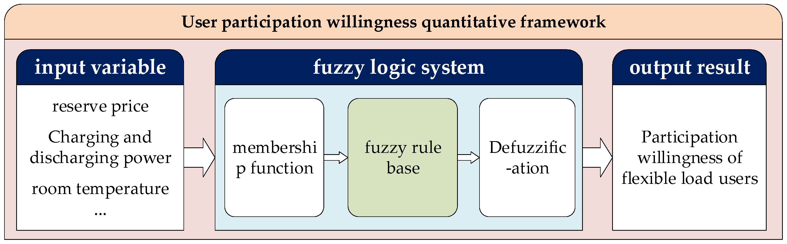
Quantifying EV and AC users’ reserve response willingness is limited by scarce real-world data and statistics under multiple factors. Inspired by [31], this paper develops a fuzzy logic–based model to quantify and characterize response willingness, tailored to the characteristics of EV and AC user groups. The specific implementation framework is shown in Figure 1.
Figure 1.
Quantitative framework for user response willingness.
The proposed framework uses multiple determinants of user willingness as input variables. These inputs are fuzzified via membership functions, evaluated through a fuzzy rule base, and then defuzzified to produce a crisp output, thereby quantitatively characterizing user willingness. Based on the resulting characterization, operators can increase willingness—and thus secure greater adjustable reserve capacity—by meeting the corresponding input conditions. Implementing the framework requires specifying (1) the input variables, (2) membership functions, (3) the fuzzy rule base, and (4) the defuzzification method.
2.1. Selection of Input Variables
EV users’ willingness to participate in reserve operation is primarily driven by economic incentives and battery safety concerns. The economic incentive is reflected in the reserve price offered by the operator as compensation for withheld capacity. Providing a reserve requires an EV aggregation to further curtail its scheduled charging/discharging power to maintain headroom and respond upon grid request, and the resulting payments offset users’ net charging cost. Safety concerns arise during reserve activation, where high-rate charging/discharging should be avoided because it may cause overcharge or over discharge, accelerate battery degradation, and compromise operational safety. Accordingly, reserve price and battery charging/discharging power are selected as the input variables for quantifying EV users’ response willingness.
AC users’ response willingness is also influenced by reserve price and, additionally, by indoor thermal comfort. Large upward or downward adjustments in air-conditioning power during reserve operation may drive indoor temperature outside the comfort range, thereby reducing user acceptance. High willingness can be maintained only if power regulation keeps indoor temperature within an acceptable comfort interval. Moreover, the width of the comfort zone constrains the feasible operating power of the air-conditioning system. Therefore, reserve price and the indoor temperature comfort zone are selected as the input variables for quantifying AC users’ response willingness.
2.2. The Realization of Fuzzy Logic System
2.2.1. Determination of Membership Function
- (1)
- Membership function of reserve price
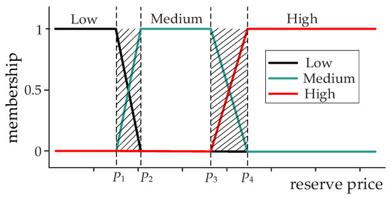
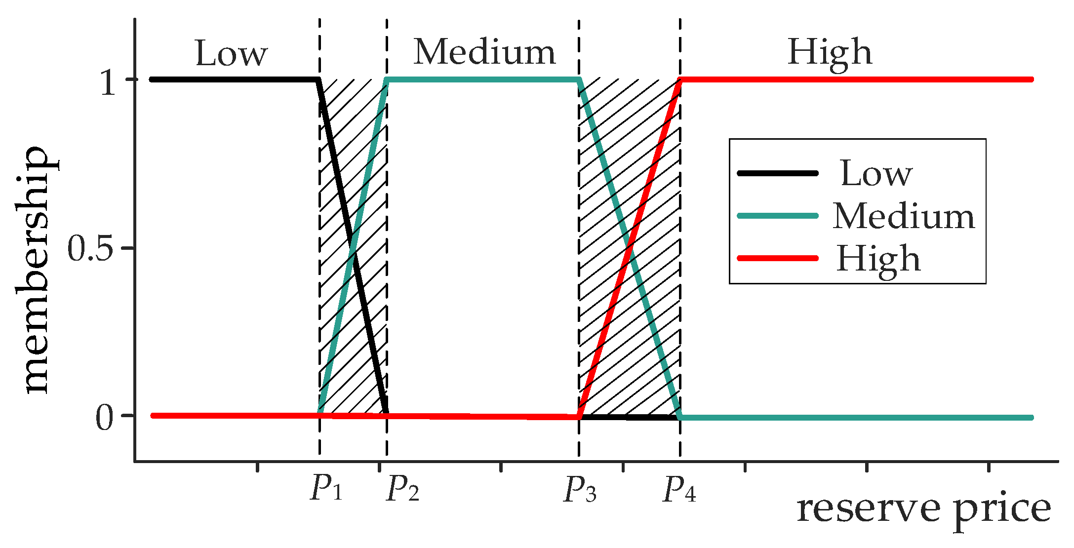
Flexible load users’ perception of the reserve price is categorized into three linguistic levels: low, medium, and high, as illustrated in Figure 2. Since users differ in their perceived thresholds for price changes, the boundary between adjacent levels is not a single value but a range across the population, corresponding to the shaded region in Figure 2. This partition is consistent with a trapezoidal transition, and so trapezoidal membership functions are adopted to fuzzify each input variable. The resulting mapping between each input variable and its fuzzy sets is shown by the solid lines in Figure 2, while the shaded region represents the transition interval of users’ perceptions.
Figure 2.
Membership function of the reserve price.
- (2)
- Membership function of battery charge and discharge power
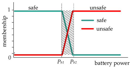
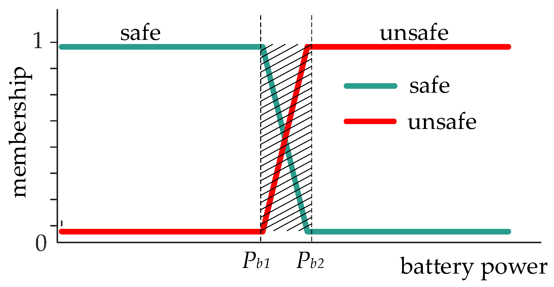
In addition to reserve price, EV users’ response willingness is influenced by battery charging and discharging power. When the charging/discharging power remains within a safe range, the battery operation is perceived as safe. During reserve provision, exceeding the safety threshold may cause overcharge or over discharge, accelerating battery degradation, and thus be perceived as unsafe. Accordingly, users’ perception of charging/discharging power is classified into two linguistic levels, safe and unsafe. The corresponding membership functions are shown in Figure 3, where the shaded region denotes the perceptual transition interval.
Figure 3.
Membership function of battery charging and discharging power.
- (3)
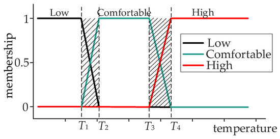
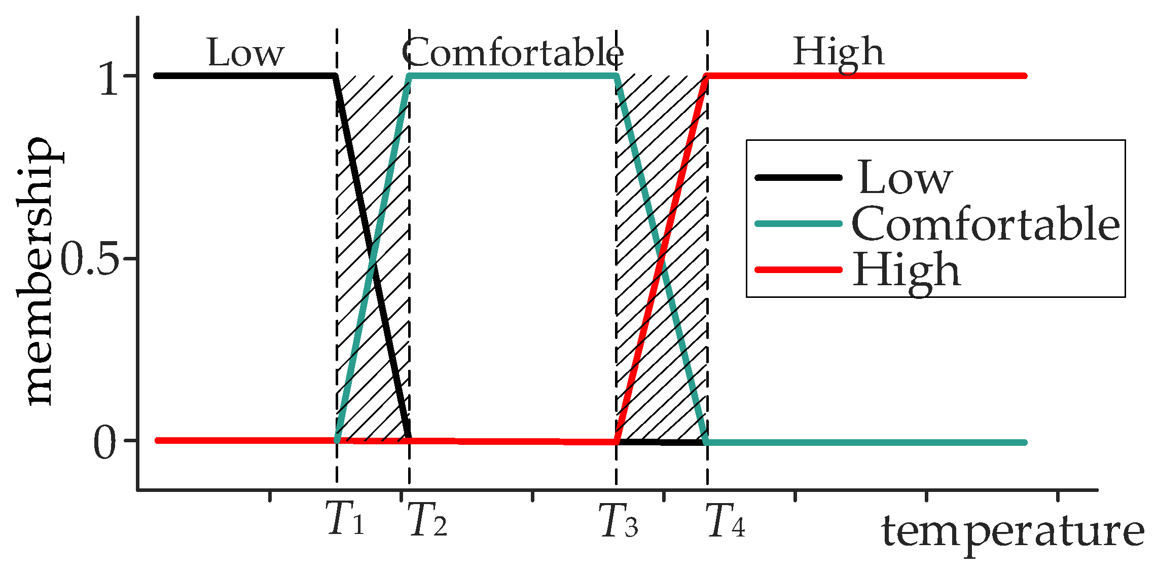
- Membership function of temperature comfort interval
In addition to reserve price, AC users’ response willingness is influenced by the indoor temperature comfort range. Deviations of indoor temperature from the comfort range reduce thermal comfort and thus lower user acceptance. Similar to reserve price perception, users’ thermal perception can be described by three linguistic levels: high temperature, comfortable temperature, and low temperature. Trapezoidal membership functions are therefore adopted to model the temperature-related fuzzy sets. The membership relations between the input variable and the fuzzy sets are shown in Figure 4.
Figure 4.
Membership function of the comfortable temperature range.
2.2.2. Fuzzy Rule Base
The fuzzy language setting of each input variable is shown in Appendix A Table A1, and the fuzzy rule base constructed for the fuzzy subset of each input variable is shown in Appendix A Table A2. In this system, the parameters of the membership function for charging/discharging prices are constructed based on the Weber–Fechner law, the parameters for current rate and depth of discharge are determined according to the Arrhenius battery dynamic aging model and the Chinese national standard GB/T 31484-2015 [32], and the response willingness threshold is set based on user behavioral characteristics and scheduling engineering practice, ensuring that all parameters have clear theoretical and engineering justifications.
2.3. Defuzzification Method and Output Results
To evaluate the performance of the fuzzy system model, the output results are clearly estimated by defuzzification methods (such as centroid, weighted average, maximum membership principle, etc.) [33]. In this study, the centroid method is used for defuzzification, and the corresponding defuzzification output results are calculated by Equation (1):
where w represents the user’s response willingness value, x denotes the input parameter, and M signifies the membership function. Based on Equation (1), defuzzification is performed to obtain a crisp output, thereby quantifying the response willingness of different flexible load user groups. To enhance user response willingness and maintain it at a high level, operators can determine the corresponding input variable range under high response willingness by selecting the threshold wy and making appropriate adjustments, as shown in Table 1.
Table 1.
Input variables under high willingness to participate.
Based on Table 1, the operator can keep different types of flexible load users in a high response-willingness state by satisfying the corresponding input conditions, including reserve price, battery charging/discharging power, and the thermal comfort range. This, in turn, increases the reserve capacity available from flexible loads.
3. Modeling Analysis of User Decision-Making Behavior Uncertainty
The operator can tune the input variable ranges to keep flexible load users in a high willingness state. In practical reserve operation, however, participation is not determined solely by subjective willingness. Even when willingness is high, users may still decline to participate, and their decisions remain uncertain. Accordingly, this section develops a quantitative method to estimate participation probability based on the relationship between response willingness and decision behavior, and then examines the resulting impacts of user decisions.
3.1. Quantification of User Decision-Making Behavior Probability
Building on the Theory of Planned Behavior (TPB), this study develops a quantitative method to estimate users’ participation probability and analyze decision uncertainty across different response-willingness states. In TPB, behavioral intention is a key predictor of the likelihood that an individual will perform a given behavior. Behavioral intention is jointly determined by attitude toward the behavior, subjective norms, and perceived behavioral control, and is typically modeled as a weighted combination of these three components [30], as shown in Equation (2):
where B represents the user’s behavior attitude, A denotes the attitude toward the behavior, S stands for subjective norms, and P signifies perceived behavioral control. The coefficients r1, r2, and r3 represent their corresponding weighting factors. In this study, the weighting coefficients are set as r1 = 0.7, r2 = 0.15, and r3 = 0.15. These values are informed by meta-analytic findings in the TPB, where attitude consistently demonstrates the strongest predictive power for behavioral intention. The specific assignment reflects the characteristics of the present application context: user decisions are primarily driven by considerations of economic benefit and battery degradation, while policy support plays a secondary role, and the full automation of response execution minimizes the relevance of perceived behavior control. The interpretation and quantification of each component are as follows. These parameter values are therefore used as scenario-specific modeling assumptions supported by the TPB-related literature and engineering reasoning, rather than empirically estimated coefficients.
3.1.1. Behavior Attitude
Behavioral attitude reflects an individual’s internal evaluation and disposition toward a specific behavior and plays a central role in decision-making. It captures both favorable and unfavorable assessments, thereby representing expected outcomes and willingness to act. In essence, behavioral attitude can be interpreted as a psychological propensity to adopt the behavior. Accordingly, for flexible load users, the TPB attitude term A is taken to be equivalent to the response willingness value w obtained from the fuzzy logic-based willingness characterization method described in Section 2. Thus, A is a continuous value between 0 and 1, directly derived from the operational parameters affecting user willingness.
3.1.2. Subjective Norm
Subjective norms describe the perceived social pressure that influences an individual’s decision to perform a behavior. Such pressure may arise from close social ties, such as relatives and friends, as well as broader contextual factors, including the social environment, policies, regulations, and cultural norms. This implies that behavioral decisions are shaped by external social influences. In the anticipated future power system scenario, demand-side flexibility and V2G technologies are expected to receive strong policy support. Therefore, the overall social and regulatory environment is assumed to be favorable to user participation, and the subjective norm value S is set to 0.8. This parameter can be adjusted by system operators to reflect the actual policy intensity and public awareness in specific regions. In this sense, the value of S should be interpreted as a scenario-specific assumption representing a favorable policy and social environment, rather than as an empirically calibrated behavioral parameter.
3.1.3. Perceived Behavior Control
Perceived behavioral control reflects an individual’s perception of the difficulty of performing a specific behavior. It is shaped by self-assessed capability and awareness of external conditions, incorporating experience, anticipated obstacles, and the individual’s actual level of control. In essence, it represents the degree of confidence in successfully carrying out the behavior. For flexible loads participating in reserve operation, execution is fully automated by intelligent control systems in accordance with dispatch instructions and requires no active user intervention. The user’s role is limited to the initial enrollment decision; all subsequent response actions are executed transparently by the automated infrastructure. Therefore, the execution process can be regarded as straightforward from the user perspective, and the confidence level in completing reserve operation can be assumed to be 100%. Accordingly, the perceived behavioral control term P is set to 1.0. Accordingly, the value of P in this study is also adopted as a scenario-specific modeling assumption under the present automation-dominant reserve response setting.
Perceived behavioral control comprises two distinct dimensions: perceived capability (the individual’s assessment of the resources and opportunities required to perform the behavior) and perceived controllability (the individual’s assessment of control over behavioral outcomes). In the proposed model, concerns regarding behavioral outcomes—such as excessive battery degradation or failure to meet charging requirements—are captured by the behavioral attitude component A, as they are directly influenced by the operational parameters that serve as inputs to the fuzzy willingness model in Section 2. Consequently, the P component in this study is narrowly defined to reflect only the perceived capability dimension. Given that reserve response execution is fully automated and requires no user intervention, the perceived capability is effectively complete. Hence, P is set to 1.0.
It should be noted that the values of S, P, and r1, r2, and r3 adopted in the TPB-based model are not empirically calibrated from large-scale behavioral datasets. Instead, they are introduced as scenario-specific modeling assumptions supported by TPB theory, the related literature, and engineering reasoning under limited data availability. Therefore, the absolute values of the estimated participation probabilities may vary under different parameter settings. Nevertheless, under reasonable parameter variations, the main qualitative conclusion of this study remains unchanged: explicitly distinguishing user willingness from actual participation probability yields a more conservative and credible reserve capacity assessment than directly equating willingness with participation probability.
3.2. Analysis of User Decision-Making Behavior
After estimating participation probability, the uncertainty of user decision-making must be characterized. For an individual EV user, the decision outcome is binary, namely, participation or non-participation, and thus follows a Bernoulli (0–1) distribution. Accordingly, the decision behavior of a single EV user is modeled as a Bernoulli random variable, with the probability mass function given by:
In the formulation, k = 1 indicates that the user participates in reserve operation, whereas k = 0 indicates non-participation. Assuming that users under the same operating mode share an identical participation probability, and that decision behaviors among individual users within the population are mutually independent, the uncertainty of group decision behavior can be characterized by a binomial distribution B(n, p). The corresponding probability mass function is as follows:
The binomial distribution captures group decisions when all users share an identical participation probability p. However, its discrete form offers limited flexibility for reserve capacity assessment and dispatch decisions. For a sufficiently large population, the central limit theorem allows the aggregate decision outcome to be approximated by a normal distribution. The approximation is given in Equations (5) and (6):
where u denotes the expected value of the number of flexible load users participating in reserve operation, and σ2 represents the corresponding variance of the decision outcomes. Equation (6) incorporates a continuity correction to reduce errors in the normal distribution approximation. The corresponding probability density function of the normal distribution is given by:
4. Reserve Capacity Evaluation Method of Flexible Loads
Building on the high-willingness operating ranges (reserve price, EV charging/discharging power, and indoor comfort band) and the participation-probability model developed in Section 2 and Section 3, this section presents a reserve capacity evaluation method for aggregated flexible loads that explicitly accounts for uncertainty in users’ participation decisions.
4.1. EV Reserve Capacity Evaluation
To evaluate the reserve capacity of an aggregated EV fleet, (i) derive feasible SOC bounds over the plug-in window, (ii) compute activation power limits under SOC constraints, and (iii) screen EVs that can provide reserve while still satisfying the required departure SOC. These steps yield an operationally feasible estimate of the EV fleet’s reserve capacity.
4.1.1. SOC Feasible Region
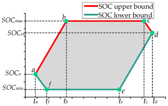
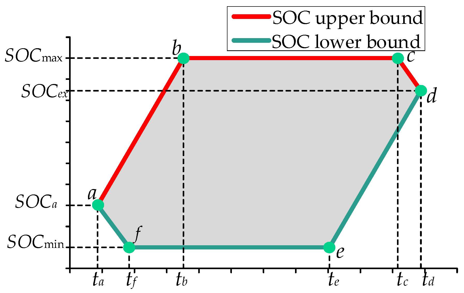
After an EV is connected to the charger, its SOC must satisfy the constraint in Equation (8) over the scheduling horizon from the interval start time ta to the unplug/departure time td.
In Equation (8), SOCa denotes the SOC at the beginning of the scheduling interval, SOCmin and SOCmax are the minimum and maximum allowable SOCs, respectively. The upper and lower SOC bounds over [ta, td] are given by Equations (9) and (10):
The boundary of SOC change of EV battery is shown in Figure 5. During the scheduling period from ta to td, the change trajectory of SOC with time can only be in the gray shadow part of the figure.
Figure 5.
EV battery SOC change boundary.
Given the user-provided information at plug-in (expected departure time, desired departure SOC/energy, and vehicle type), the characteristic time instants in Figure 5 can be computed. Their definitions and calculation formulas are summarized in Table 2.
Table 2.
Definition and calculation of characteristic time instants.
4.1.2. Activation Power Limits
During reserve activation, the deliverable charging/discharging power depends on (i) the operating power limits associated with high user willingness and (ii) the instantaneous battery SOC. The SOC-dependent limits are derived as follows.
(1) Upward reserve activation (discharging). The EV discharges to the grid and must sustain the response throughout the scheduling interval without violating SOCmin. The maximum discharging power satisfies the following constraint:
(2) Downward reserve activation (charging). The EV absorbs power from the grid and must sustain the response throughout the scheduling interval without exceeding SOCmax. The maximum charging power satisfies the following constraint:
Accordingly, when an EV is scheduled to provide reserve, its SOC-constrained maximum power is computed by Equation (13).
4.1.3. Screening EVs Eligible for Reserve Service
An EV providing reserve must still meet the user’s departure requirement. Because the next interval may call either upward or downward reserve, each EV is screened to ensure it can participate in the current interval while guaranteeing that its SOC can still be restored to the expected departure SOC by td. EVs that fail this check are treated as conventional charging loads until departure. The screening rules are as follows.
(1) Assume that the current scheduling period requires a downward reserve response and that the EV is assigned a low charging power (down to 0). At the end of the scheduling period, the real-time state of charge of the EV, SOCch,end, equals the initial state of charge SOCa at the beginning of the period, as given in (14). The minimum charging time tc,min required to increase the SOC from SOCch,end to SOCex is calculated by (15). If tc,min exceeds the available time from the end of the scheduling period to the expected departure time td, the EV may fail to reach the target SOC, SOCex, before td, and thus cannot satisfy the user’s charging requirement. In this case, the EV is not allowed to participate in the downward reserve operation during the current period. Therefore, participation in the downward reserve operation must satisfy (16).
(2) Assume that the current scheduling period requires an upward reserve response and that the EV discharges at the maximum power Pdis,max. The real-time state of charge at the end of the scheduling period, SOCdis,end, is obtained from (17). The minimum charging time td,min required to increase the SOC from SOCdis,end to SOCex is calculated by (18). If td,min exceeds the available time from the end of the scheduling period to the expected departure time td, the EV may fail to reach SOCex before td and thus cannot satisfy the user’s charging requirement. In this case, the EV is not allowed to participate in the upward reserve operation during the current period. Therefore, participation in the upward reserve operation must satisfy (19).
Based on the above two cases, the feasibility of EV participation in reserve operation is determined by (9) and (12). Accordingly, the number of EVs that can participate in reserve operation during the current period can be identified.
4.1.4. EV Reserve Capacity Evaluation
After determining the number of electric vehicles (EVs) that can participate in reserve operations and their corresponding maximum power limits, the total adjustable capacity of EVs during their residence time at the charging station can be obtained. This adjustable capacity can be utilized for both scheduling and reserve operations. Based on the scheduled charging power PEV, the upward and downward reserve capacities that can be provided by a single EV are given by (20).
In this expression, represents the upward reserve capacity of the i-th EV, while represents its downward reserve capacity. Accordingly, the theoretical reserve capacity aggregated from an EV cluster can be calculated as follows:
4.2. AC Reserve Capacity Evaluation
4.2.1. AC Operating Model
The operating behavior of an air-conditioning (AC) load is influenced by multiple factors (e.g., indoor/outdoor temperature, humidity, and room characteristics). To obtain a tractable state equation, the model in [34] is adopted and simplified as follows:
where Pair,t denotes the steady-state AC power when the indoor temperature is stabilized; Tout,t and Tset,t are the outdoor temperature and AC setpoint, respectively; a is the equivalent thermal conductivity of the room; ηair is the energy efficiency ratio of the inverter AC; Tin,t−1 and Tin,t are the indoor temperatures at the previous and current instants; Δtair is the time step; R is the equivalent thermal resistance; and c is the equivalent thermal capacitance. Based on (23), the indoor temperature trajectory under a given AC power during a scheduling interval can be calculated.
4.2.2. AC Operating Power Limits
To maintain high user response willingness, the reserve operation must satisfy the user’s thermal comfort band. The comfort constraint directly restricts the feasible AC response power in the current scheduling period. Moreover, because reserve activation requires sustained response, the indoor temperature must remain within limits throughout the response window. Therefore, by combining (23) with the comfort band, the feasible AC power bounds are derived and then used to correct the AC reserve capacity.
(1) Indoor temperature evolution during reserve response
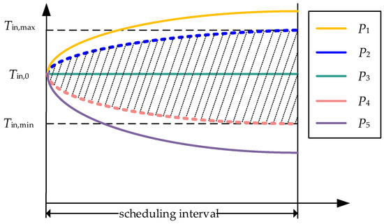
After receiving a reserve activation signal, the AC adjusts its power and sustains the response over the scheduling interval while keeping indoor temperature within the comfort band. The temperature dynamics follow (23). Figure 6 illustrates the indoor temperature trajectories for a 1 h operation under different power levels.
Figure 6.
AC load different power operation curve.
In Figure 6, Tin,max and Tin,min are the upper and lower comfort limits, respectively, and Tin,0 is the initial indoor temperature. Pt,lb denotes the minimum power that keeps the indoor temperature at (or below) the upper comfort limit after 1 h under the current indoor/outdoor conditions (i.e., the lower bound of the adjustable power range). Pt,ub denotes the power that keeps the indoor temperature at (or above) the lower comfort limit after 1 h (i.e., the upper bound of the adjustable power range).
(2) Upper and lower bounds of AC cooling power
Under the comfort band corresponding to high willingness, the bounds of AC cooling power are defined as follows.
- Upper bound of cooling power: the continuous operating power Pi,ub that drives the indoor temperature to 24 °C after 1 h, given the current indoor and outdoor temperatures.
- Lower bound of cooling power: the continuous operating power Pi,lb that drives the indoor temperature to 26 °C after 1 h, given the current indoor and outdoor temperatures. The downward adjustment of cooling power is not allowed, i.e., Pi,lb ≥ 0.
4.2.3. AC Reserve Capacity Evaluation
Once the feasible operating power bounds are obtained, the adjustable capacity of an AC load can be determined. Similar to EVs, given the scheduled AC power Pa, the upward and downward reserve capacities of a single AC unit are computed by:
Accordingly, the aggregated theoretical reserve capacity of an AC cluster is:
4.3. Reserve Capacity Evaluation Considering User Decision-Making Behavior
After deriving the reserve capacity model for a single flexible load, group-level reserve capacity assessment must account for uncertainty in user decision-making. Specifically, not all flexible loads will choose to participate in reserve operation. To adjust the aggregated theoretical reserve capacity, a decision-outcome proportionality coefficient k is introduced:
where N is the number of flexible loads connected to the grid and Nre is the number that actually participate in reserve operation. Since Nre follows the normal approximation in (7), k can also be modeled as a normally distributed random variable. The theoretical reserve capacity is then corrected by k, yielding:
5. Optimal Reserve Operation of the Distribution Network with Flexible Loads
5.1. Objective Function
From the perspective of the distribution network operator, flexible loads are dispatched as reserve resources. In the day-ahead stage, scheduling decisions are made based on the next-day forecasts of generation, load, and the reserve capacities of flexible loads, with the goal of minimizing the total operating cost while exploiting flexible-load reserve potential to maintain power balance and facilitate renewable energy utilization.
The operating cost includes: main-grid purchase cost F1, network loss cost F2, renewable energy purchase cost F3, flexible-load scheduling cost F4, and reserve capacity cost F5. The total cost is:
where Cg is the unit price of electricity purchased from the main grid; Pg,t is the power imported from the main grid at time t. Closs is the unit loss cost; ELine is the branch set; Iij,t is the current on branch ij at time t; and rij is the branch resistance. Cres is the unit purchase price of renewable energy, and Cc,res is the penalty unit cost for renewable curtailment. Pre and Pact are the predicted and actual renewable outputs at time t, respectively. Cc and Cd are the unit costs for EV charging and discharging in scheduling, respectively; Ca is the electricity price for AC scheduling. Pc,ev and Pd,ev are EV charging and discharging powers, respectively; Pa is the scheduled AC power. CR,ev is the unit price of EV reserve; Rev,+ and Rev,- are the realized upward and downward reserve responses of EVs. CRa is the unit price of AC reserve; Rac,+, and Rac,- are the realized upward and downward reserve responses of ACs.
5.2. Constraints
5.2.1. Network Power-Flow Security Constraints
The conventional branch power-flow model is nonlinear. To enable efficient optimization, second-order conic relaxation (SOCR) is applied to obtain a convex form solvable by standard solvers [35]. The SOCR-based network constraints are:
where Pj,t and Qj,t are the net active and reactive injections at node j and time t, respectively; Pjk,t and Qjk,t are the active and reactive power flows from node j to node k at time t; xij is the branch reactance; lij,t is the squared branch current magnitude; and vi,t is the squared node voltage magnitude. Vi,min and Vi,max are the allowable voltage limits, and Iij,max is the branch current limit.
5.2.2. Renewable Output Constraints
5.2.3. Conventional Operating Constraints of Flexible Loads
Because user decision uncertainty is considered, the theoretically feasible power bounds of flexible-load clusters are corrected using the decision-outcome coefficient k. The revised conventional operating constraints are:
where rc and rd are binary variables indicating EV charging and discharging states, respectively.
5.2.4. Reserve Operation Constraints of Flexible Loads
With user decision uncertainty, reserve constraints for flexible loads are formulated as:
where k1 and k2 are the reserve coefficients of the corresponding base load, respectively.
5.2.5. Chance-Constrained Uncertainty Transformation
Using a chance-constrained formulation, uncertain constraints in flexible-load operation are expressed probabilistically under a specified confidence level:
where α is the acceptable violation probability for each constraint. When the underlying random variables are modeled as normally distributed, (35) can be transformed into a deterministic equivalent based on the confidence level, enabling solver-based computation:
where φ−1 is the inverse cumulative distribution function of the standard normal distribution; uev and uac are the expected numbers of EV and AC users participating in the reserve operation, respectively; and σ2ev and σ2ac are the corresponding variances.
6. Case Study
6.1. Example Setting and Basic Data
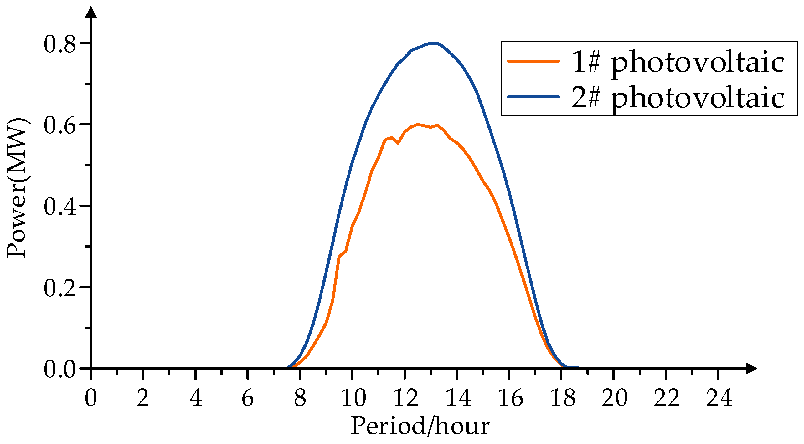
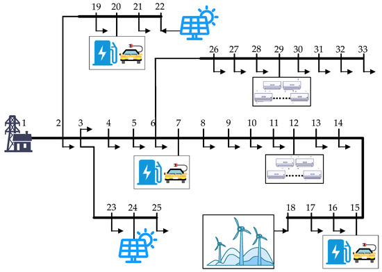
Based on the improved IEEE 33-bus distribution network, the example setting is carried out. The IEEE 33-bus network topology, including wind farm, photovoltaic, EV charging station, and air conditioning load access, is shown in Figure 7, and the day-ahead optimal scheduling of the distribution network is carried out. The EV sample parameters are obtained from public measured data of mainstream electric vehicle models. The AC load samples are set according to typical building thermal parameters in South China. The wind and PV power output data are derived from actual measured operation data of a regional distribution network in the China Southern Power Grid. The optimization model is solved with a relative MIP gap of 0.5%. The electricity purchase cost, reserve cost, and time-of-use price are set based on the actual market price standards of the China Southern Power Grid and typical engineering specifications.
Figure 7.
The modified IEEE 33-bus distribution network.
To validate the feasibility and effectiveness of the proposed method in practical applications, the following case studies (denoted as C1–C6) are established for comparative analysis. Each case is explicitly labeled with its attribute and validation purpose, as follows:
C1: Proposed method. Reserve pricing, battery power limits, and thermal comfort bands for flexible loads are set based on high user responsiveness. Confidence level: 95%.
C2: Alternative method—traditional reserve scheduling. Reserve pricing, battery power limits, and thermal comfort bands are set without considering user responsiveness. Confidence level: 95%. It is a typical traditional engineering-oriented reserve strategy, used to compare with the proposed strategy and highlight the value of considering user responsiveness.
C3: Alternative method—deterministic scheduling. Reserve pricing, battery power limits, and thermal comfort bands for flexible loads are set based on high user responsiveness, without considering user decision-making uncertainty. It is used to verify the necessity of considering user decision uncertainty in reserve scheduling.
C4: Sensitivity analysis—confidence level 90%. Parameters are set based on high user responsiveness (same as C1). Confidence level: 90%. It is part of the sensitivity analysis group, used to investigate the impact of different confidence levels on scheduling results.
C5: Sensitivity analysis—confidence level 85%. Parameters are set based on high user responsiveness (same as C1). Confidence level: 85%.
C6: Baseline case—no reserve participation. EVs and ACs operate only as conventional loads without participating in reserve scheduling. It serves as the fundamental baseline of this study, used to verify the practical value of flexible loads participating in reserve scheduling.
Through the example results, the user response willingness value, flexible load reserve capacity, and overall economic benefits under each example are analyzed.
6.2. Results
6.2.1. User’s Response Willingness Value and Decision Behavior Probability
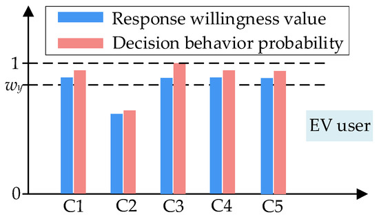
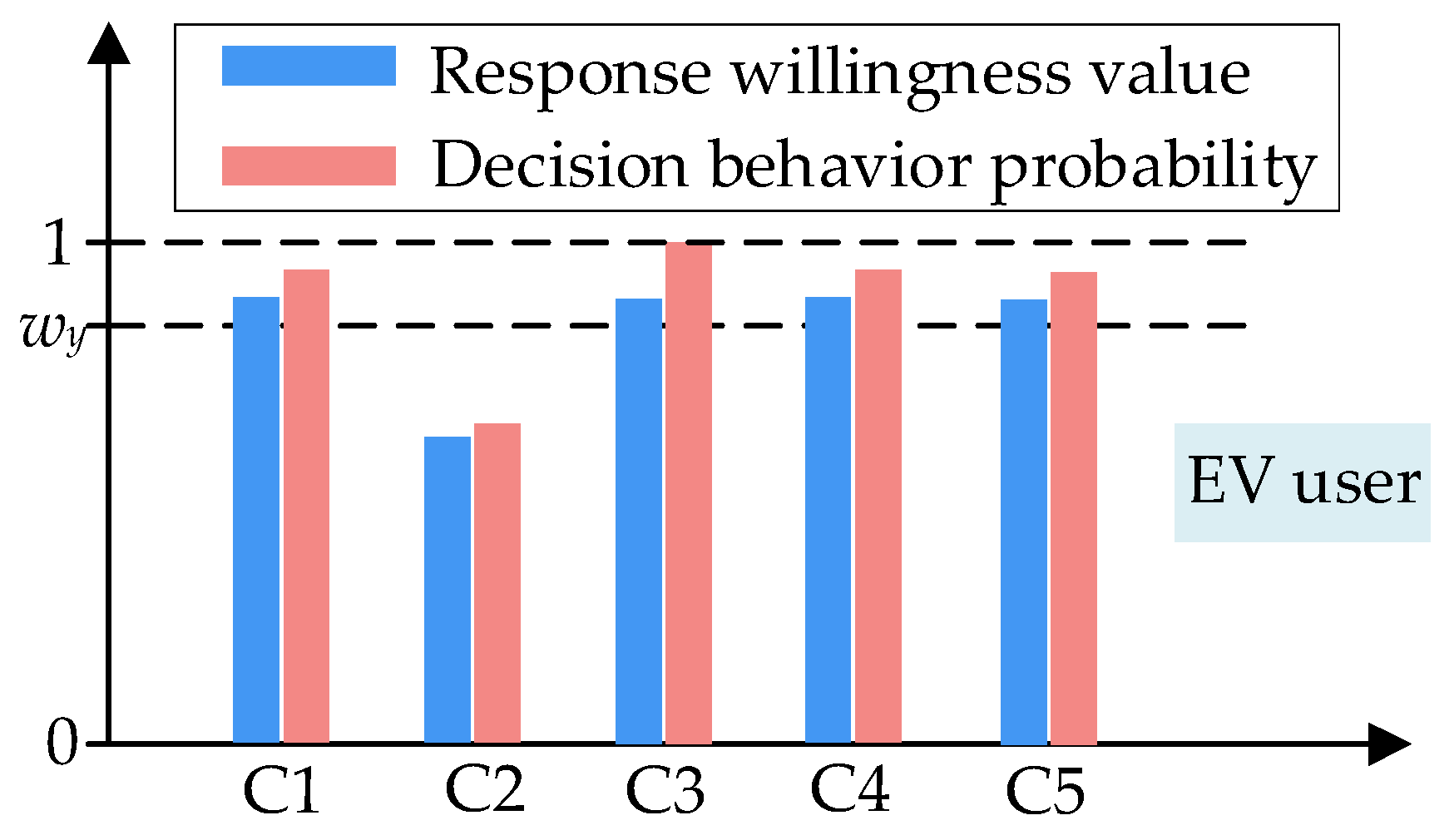
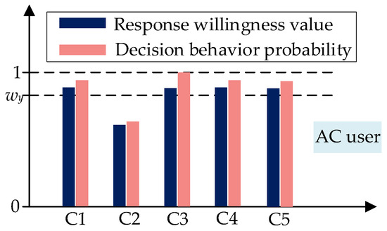
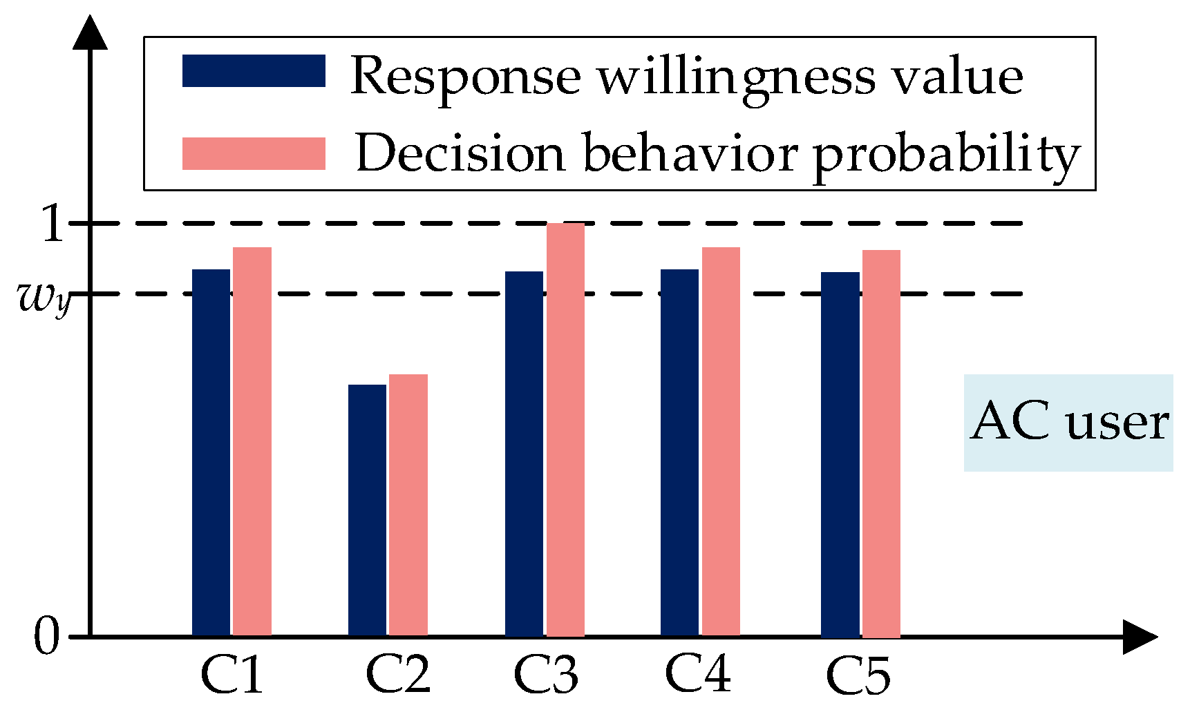
The proposed user response willingness evaluation framework is applied to quantify the willingness-to-respond of flexible load users in Cases C1–C4. Based on the quantified willingness levels, the corresponding user decision-making behavior probabilities are derived. The results for EV users and AC users are illustrated in Figure 8 and Figure 9, respectively.
Figure 8.
EV user response willingness value and decision behavior probability.
Figure 9.
AC user response willingness value and decision behavior probability.
As shown in Figure 8 and Figure 9, the reserve operation parameter settings in Cases C1, C3, C4, and C5 are consistent with the psychological expectations of flexible load users. Consequently, both the response willingness values and the corresponding decision-making behavior probabilities remain at relatively high levels, and their trends are generally consistent across these cases. In contrast, Case C2 exhibits significantly lower response willingness values and decision-making behavior probabilities. This reduction is primarily attributed to the lower reserve price, which weakens user economic incentives, as well as the absence of strict constraints on battery operating power and temperature comfort intervals. These factors jointly decrease user acceptance of reserve participation. In Case C3, all users in the high willingness state are assumed to participate in reserve operation. Therefore, the corresponding decision-making behavior probability is set to 1.
6.2.2. Reserve Capacity Boundary of Flexible Load
Based on the case settings, the reserve capacity boundaries of flexible loads are analyzed from two perspectives. The first focuses on the impact of user response willingness and decision-making behavior. The second examines the influence of different confidence level settings.
(1) Reserve capacity boundaries considering user willingness and behavior
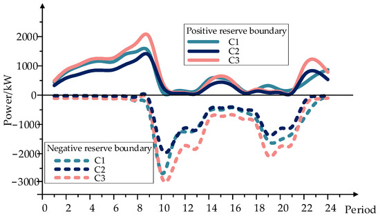
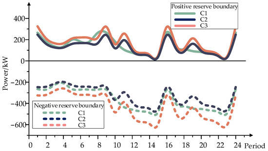
To evaluate the impact of user response willingness and decision-making behavior on reserve capacity boundaries, the maximum reserve capacities of EVs and AC loads are calculated under Cases C1, C2, and C3. The corresponding results are shown in Figure 10 and Figure 11.
Figure 10.
The reserve capacity boundary of EV under C1, C2, and C3.
Figure 11.
The reserve capacity boundary of AC under C1, C2, and C3.
As illustrated in Figure 10 and Figure 11, a comparison between Cases C1 and C3 shows that both cases share identical operational parameter settings and user response willingness levels. However, Case C1 explicitly accounts for the uncertainty in user decision-making behavior. This consideration leads to a smaller number of flexible loads participating in reserve operation. As a result, the practically available reserve capacity boundary in Case C1 is lower than that in Case C3. When comparing Cases C1 and C2, although Case C2 allows wider battery operating power ranges and broader thermal comfort intervals, the user decision-making behavior probability is significantly lower. Consequently, fewer flexible loads choose to participate in reserve operation. This results in a smaller reserve capacity boundary in Case C2 compared to Case C1.
(2) Reserve capacity boundary under different confidence settings
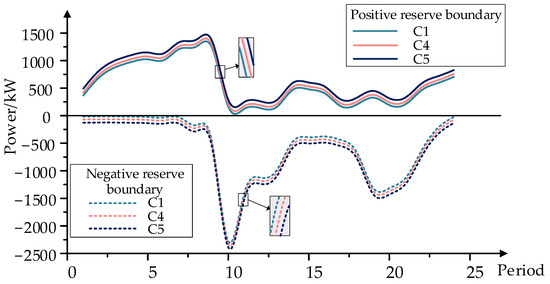
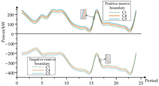
To analyze the effect of confidence level settings on reserve capacity boundaries, the maximum reserve capacities of EVs and AC loads are evaluated under Cases C1, C4, and C5. The results are presented in Figure 12 and Figure 13.
Figure 12.
The reserve capacity boundary of EV under C1, C4 and C5.
Figure 13.
The reserve capacity boundary of AC under C1, C4, and C5.
As shown in Figure 12 and Figure 13, the reserve capacity boundaries of flexible loads increase as the confidence level decreases. A lower confidence level indicates that the system operator adopts a less conservative estimation of the number of flexible loads available for reserve operation. This reflects an assumption that a larger proportion of flexible loads will participate in reserve services.
6.2.3. Economic Benefit Analysis
The economic performance of each case is summarized in Table 3. The net electricity purchase cost of EV users represents the actual charging payment after participating in reserve-optimized operation, while the net electricity purchase cost of AC users denotes the corresponding air-conditioning electricity expenditure.
Table 3.
Economic performance results.
As shown in Table 3, incorporating flexible loads into reserve-optimized operation yields clear economic benefits. Compared with the benchmark Case C6 (no flexible load participation), the proposed framework in Case C1 reduces the distribution network’s total operating cost by 3.0% (from 41,667.28 to 40,424.31 USD). For end-users, EV users see a 41.6% reduction in net electricity purchase costs (from 4430.54 to 2097.79 USD), while AC users achieve a 23.2% reduction (from 8487.07 to 6494.03 USD), driven by reserve incentives.
Case C2 yields the lowest reserve cost (891.66 USD) due to operator-favorable reserve prices, which reduce network operating costs. However, these settings weaken user incentives: compared to C1, reserve cost in C2 is 19.9% lower, but user participation drops significantly, leading to insufficient flexible reserve capacity and increased reliance on high-cost backup resources, creating a trade-off between short-term cost reduction and long-term operational reliability.
A comparison between Cases C1 and C3 indicates that ignoring user decision uncertainty (C3) enables a larger adjustable capacity but leads to 10.6% higher AC user costs (from 6494.03 to 7217.69 USD) and a 1.8% increase in overall operating cost (from 40,424.31 to 41,165.92 USD). Moreover, ignoring uncertainty risks dispatching power beyond operational limits, raising operational risk.
Results from Cases C1, C4, and C5 show that confidence levels have a limited impact on economic outcomes. Nevertheless, the higher confidence level in C1 enhances the over-all security of reserve operations without significantly increasing costs.
Overall, Case C1 achieves a better balance among economic efficiency (3.0% total cost reduction), user participation (via significant user cost reductions), and operational reliability (via uncertainty-aware scheduling and higher confidence levels). This systematic trade-off demonstrates the practical advantages of the proposed method for grid operators in reserve operation applications.
7. Conclusions
This study proposes a user willingness-aware framework for evaluating the reserve capacity of flexible loads, with a focus on electric vehicles (EVs) and air conditioning (AC) systems. A fuzzy logic-based model is developed to quantify user response willingness under multiple influencing factors. Building upon this, the theory of planned behavior is incorporated to probabilistically characterize user decision-making, thereby addressing behavioral uncertainties in reserve provision.
The proposed method is embedded into a distribution network reserve optimization model, and validated through case studies. The main findings are summarized as follows:
(1) The reserve capacity evaluation model explicitly incorporates user response willingness. By respecting users’ operational preferences, it maintains a high level of willingness across the participant pool. This approach encourages greater user engagement in reserve services, thereby securing more substantial and reliable reserve capacity for the grid.
(2) A probabilistic model of user decision-making is established based on the theory of planned behavior. This method avoids the oversimplification of equating willingness directly with participation probability. As a result, more objective and behaviorally realistic inputs are provided for reserve capacity assessment and scheduling decisions.
(3) The proposed evaluation mechanism jointly considers user willingness and sustainable response duration. It ensures that flexible load operating limits are respected while preserving high user engagement. Integrated with the decision probability model, it forms operational constraints that enhance the safety and reliability of reserve dispatch in distribution networks.
From the perspective of practical application, the proposed framework can provide direct decision support for distribution network operators. By combining willingness-aware operating conditions with probabilistic participation modeling, operators can identify reserve pricing and operating ranges that better sustain user participation, estimate more credible reserve capacity under uncertainty, and determine reserve scheduling schemes that balance economic efficiency, user acceptance, and operational reliability.
It should be noted that the proposed probabilistic model for user decision-making adopts two simplifications: users within the same group are assumed to have identical participation probabilities, and individual user decisions are assumed to be mutually in-dependent. These assumptions are adopted to ensure computational tractability and to highlight the core logic of the proposed framework. In practical scenarios, however, user participation probabilities may differ due to individual heterogeneity, such as consumption habits, battery conditions, and comfort preferences. Meanwhile, user decisions may exhibit temporal correlation under the same price signals or grid dispatch instructions. Further, while the validation on the IEEE 33-bus system demonstrates the method’s effectiveness, broader testing on larger networks and with real-world data is warranted to further establish generalizability. In future research, more detailed user classification, heterogeneous probability modeling, and spatiotemporal correlation of decision behaviors will be taken into account to further enhance the realism and applicability of the model. In addition, future research will further calibrate the TPB-related parameters using questionnaire data, field observations, and historical participation records, so as to enhance the empirical grounding of the behavioral layer.
Author Contributions
Conceptualization, Z.O., L.Q., S.P. and W.D.; Methodology, Z.O., H.S. and W.D.; Software, W.W., L.Z. and M.F.; Validation, Z.O., C.H., H.S. and W.D.; Formal analysis, L.Q., S.P. and W.W.; Resources, Z.O., L.Q., S.P. and W.W.; Data curation, M.F., C.H. and H.S.; Writing—original draft, Z.O., L.Q. and S.P.; Writing—review and editing, L.Z., H.S. and W.D.; Visualization, L.Z., M.F. and H.S.; Funding acquisition, Z.O., L.Q. and S.P. All authors have read and agreed to the published version of the manuscript.
Funding
This work is supported by the Science and Technology Project of China Southern Power Grid (GDKJXM20231509).
Data Availability Statement
The data supporting this study cannot be made publicly available due to privacy and confidentiality restrictions imposed by power grid operators.
Conflicts of Interest
Authors Zhongxi Ou, Lihong Qian, Liang Zhang, Mingqian Feng, and Chuyuan Hong were employed by the Guangdong Zhuhai Power Supply Bureau. Authors Sui Peng and Weijie Wu were employed by the Guangdong Power Grid Corporation. The remaining authors declare that the research was conducted in the absence of any commercial or financial relationships that could be construed as a potential conflict of interest. The authors declare that this study received funding from China Southern Power Grid. The funder was not involved in the study design, collection, analysis, interpretation of data, the writing of this article or the decision to submit it for publication.
Appendix A
Table A1.
Input variable fuzzy language.
Table A2.
Fuzzy rules related to EV users.
Table A3.
AC user-related fuzzy rules.
Table A4.
Time of use pricing.
Table A5.
Other parameter data.
For improved reproducibility, the key numerical parameters of all membership functions are listed below:
- Reserve price: low when the price is less than 0.06 $/kWh; medium when the price ranges from 0.08 to 1 $/kWh; high when the price is higher than 0.12 $/kWh.
- Battery charging/discharging power: safe when the C-rate is within 0 to 0.95; unsafe when the C-rate exceeds 1.
- Temperature comfort zone: comfortable when the temperature is between 24 °C and 26 °C; high when the temperature is above 27 °C; low when the temperature is below 23 °C.
Figure A1.
Wind farm output.
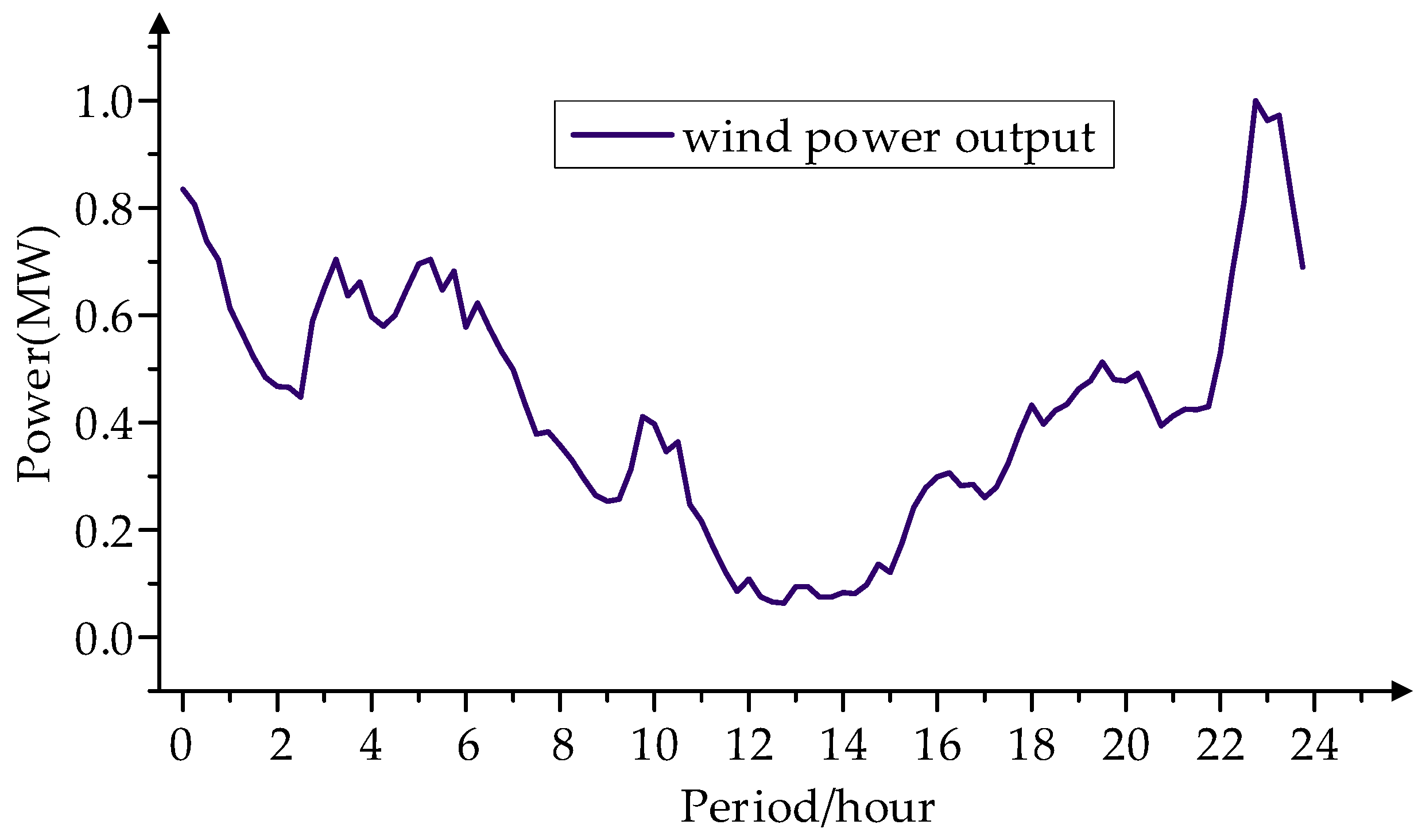
Figure A2.
Photovoltaic plant output.
References
- Gielen, D.; Boshell, F.; Saygin, D.; Bazilian, M.D.; Wagner, N.; Gorini, R. The role of renewable energy in the global energy transformation. Energy Strategy Rev. 2019, 24, 38–50. [Google Scholar] [CrossRef] [Scilit]
- Ourahou, M.; Ayrir, W.; Hassouni, B.E.; Haddi, A. Review on smart grid control and reliability in presence of renewable energies: Challenges and prospects. Math. Comput. Simul. 2020, 167, 19–31. [Google Scholar] [CrossRef] [Scilit]
- Lu, H.; Wang, C.; Li, Q.; Wiser, R.; Porter, K. Reducing wind power curtailment in China: Comparing the roles of coal power flexibility and improved dispatch. Clim. Policy 2019, 19, 623–635. [Google Scholar] [CrossRef] [Scilit]
- Hungerford, Z.; Bruce, A.; MacGill, I. The value of flexible load in power systems with high renewable energy penetration. Energy 2019, 188, 115960. [Google Scholar] [CrossRef] [Scilit]
- Goel, S.; Sharma, R.; Rathore, A.K. A review on barrier and challenges of electric vehicle in India and vehicle to grid optimisation. Transp. Eng. 2021, 4, 100057. [Google Scholar] [CrossRef] [Scilit]
- Liu, J.; Zhuge, C.; Tang, J.H.C.G.; Meng, M.; Zhang, J. A spatial agent-based joint model of electric vehicle and vehicle-to-grid adoption: A case of Beijing. Appl. Energy 2022, 310, 118581. [Google Scholar] [CrossRef] [Scilit]
- Ai, X.; Wu, Z.; Hu, J.; Li, Y.; Hou, P. Robust operation strategy enabling a combined wind/battery power plant for providing energy and frequency ancillary services. Int. J. Electr. Power Energy Syst. 2020, 118, 105736. [Google Scholar] [CrossRef] [Scilit]
- Sovacool, B.K.; Axsen, J.; Kempton, W. The future promise of vehicle-to-grid (V2G) integration: A sociotechnical review and research agenda. Annu. Rev. Environ. Resour. 2017, 42, 377–406. [Google Scholar] [CrossRef] [Scilit]
- Habib, S.; Kamran, M.; Rashid, U. Impact analysis of vehicle-to-grid technology and charging strategies of electric vehicles on distribution networks—A review. J. Power Sources 2015, 277, 205–214. [Google Scholar] [CrossRef] [Scilit]
- Huang, X.; Liu, Y.; Shen, F.; Gao, S.; Gu, Y.R.; Yang, Z.X.; Wen, X. Vehicle-to-grid interaction: Review and prospects. Autom. Electr. Power Syst. 2024, 48, 3–23. [Google Scholar] [CrossRef]
- Sarker, M.R.; Pandžić, H.; Sun, K.; Ortega-Vazquez, M.A. Optimal operation of aggregated electric vehicle charging stations coupled with energy storage. IET Gener. Transm. Distrib. 2018, 12, 1127–1136. [Google Scholar] [CrossRef] [Scilit]
- Zhang, H.; Hu, Z.; Xu, Z.; Song, Y. Evaluation of achievable vehicle-to-grid capacity using aggregate Pev model. IEEE Trans. Power Syst. 2016, 32, 784–794. [Google Scholar] [CrossRef] [Scilit]
- Wang, J.; Jia, Y.; Mi, Z.; Chen, H.; Fang, H. Reserve service strategy of electric vehicles based on double-incentive mechanism. Autom. Electr. Power Syst. 2020, 44, 68–76. [Google Scholar] [CrossRef]
- Jiang, J.; Teng, X.; Zhang, Y.; Tu, M.; Guan, L. Co-optimization Model of Energy and Auxiliary Service Market Considering Opportunity Cost. In Proceedings of the 2020 IEEE Sustainable Power and Energy Conference (iSPEC), Chengdu, China, 23–25 November 2020; IEEE: Piscataway, NJ, USA, 2020; pp. 1094–1099. [Google Scholar] [CrossRef] [Scilit]
- Gupta, V.; Kumar, R.; Panigrahi, B.K. User-willingness-based decentralized EV charging management in multiaggregator scheduling. IEEE Trans. Ind. Appl. 2020, 56, 5704–5715. [Google Scholar] [CrossRef] [Scilit]
- Junjie, H.; Wenshuai, M.; Yusheng, X.; Li, Y.; Dongliang, X. Quantification of reserve capacity provided by electric vehicle aggregator based on framework of cyberphysical-social system in energy. Autom. Electr. Power Syst. 2022, 46, 46–54. [Google Scholar] [CrossRef]
- Geske, J.; Schumann, D. Willing to participate in vehicle-to-grid (V2G)? Why not! Energy Policy 2018, 120, 392–401. [Google Scholar] [CrossRef] [Scilit]
- Fang, Y.; Hu, J.; Ma, W. Master–slave game optimal dispatch strategy for EV aggregators considering user willingness. Trans. China Electrotech. Soc. 2024, 39, 5091–5103. [Google Scholar] [CrossRef]
- Hou, H.; Wang, Y.; Chen, Y.; Zhao, B.; Zhang, L.; Xie, C. Long-time scale vehicle-to-grid scheduling strategy considering psychological effect based on Weber-Fechner law. Int. J. Electr. Power Energy Syst. 2022, 136, 107709. [Google Scholar] [CrossRef] [Scilit]
- Chen, Z.; Li, Y.Q.; Leng, Z.Y.; Lu, G.X. Refined modeling and energy management strategy of typical household high-power loads. Autom. Electr. Power Syst. 2018, 42, 135–143. [Google Scholar] [CrossRef]
- Song, M.; Gao, C.; Yan, H.; Yang, J. Thermal battery modeling of inverter air conditioning for demand response. IEEE Trans. Smart Grid 2017, 9, 5522–5534. [Google Scholar] [CrossRef] [Scilit]
- Wang, J.; Redondo, N.; Galiana, F. Demand-side reserve offers in joint energy/reserve electricity markets. IEEE Trans. Power Syst. 2003, 18, 1300–1306. [Google Scholar] [CrossRef] [Scilit]
- Cui, W.; Ding, Y.; Hui, H.; Lin, Z.; Du, P.; Song, Y.; Shao, C. Evaluation and sequential dispatch of operating reserve provided by air conditioners considering lead–lag rebound effect. IEEE Trans. Power Syst. 2018, 33, 6935–6950. [Google Scholar] [CrossRef] [Scilit]
- Cheng, D.; Zhang, W.; Wang, K. Hierarchical reserve allocation with air conditioning loads considering lock time using Benders decomposition. Int. J. Electr. Power Energy Syst. 2019, 110, 293–308. [Google Scholar] [CrossRef] [Scilit]
- Li, N.; Wang, X. Research of air conditioners providing frequency controlled reserve for microgrid. Power Syst. Prot. Control 2015, 43, 101–105. [Google Scholar] [CrossRef]
- Conte, F.; Massucco, S.; Silvestro, F. Frequency control services by a building cooling system aggregate. Electr. Power Syst. Res. 2016, 141, 137–146. [Google Scholar] [CrossRef] [Scilit]
- Ma, W.; Hu, J.; Fang, Y.; Wu, J.A.; Xie, D.L.; Xue, Y.S. Multi-agent representation of electric vehicle users’ willingness to participate in regulation and quantification of credible capacity. Autom. Electr. Power Syst. 2023, 47, 122–131. [Google Scholar] [CrossRef]
- Liu, K.; Liu, Y. Incentive-willingness-decision framework: Unit discharge triangle-based maximum stable V2G capability evaluation. Appl. Energy 2024, 374, 123850. [Google Scholar] [CrossRef] [Scilit]
- Chen, T.; Yang, R.; Sui, K.; Dong, P. Electric vehicle charging-station user participation optimization considering user decision uncertainty. J. Electr. Power Sci. Technol. 2024, 39, 128–137. [Google Scholar] [CrossRef]
- Ajzen, I. The theory of planned behavior. Organ. Behav. Hum. Decis. Process. 1991, 50, 179–211. [Google Scholar] [CrossRef] [Scilit]
- Selvachandran, G.; Quek, S.G.; Lan, L.T.H.; Son, L.H.; Giang, N.L.; Ding, W.; Abdel-Basset, M.; de Albuquerque, V.H.C. A new design of mamdani complex fuzzy inference system for multiattribute decision making problems. IEEE Trans. Fuzzy Syst. 2019, 29, 716–730. [Google Scholar] [CrossRef] [Scilit]
- GB/T 31484-2015; Cycle Life Requirements and Test Methods for Traction Battery of Electric Vehicle. China Standards Press: Beijing, China, 2015.
- Ross, T.J. Fuzzy Logic with Engineering Applications, 2nd ed.; John Wiley & Sons: Chichester, UK, 2010. [Google Scholar]
- Yang, X.; Lu, W.; Yu, W.; Chen, Y.G.; Cao, J.B. Optimal dispatching and control strategies for residential load of intelligent communities. Power Syst. Prot. Control 2023, 51, 22–34. [Google Scholar] [CrossRef]
- Gao, H.; Liu, J.; Wang, L. Robust coordinated optimization of active and reactive power in active distribution systems. IEEE Trans. Smart Grid 2017, 9, 4436–4447. [Google Scholar] [CrossRef] [Scilit]

Disclaimer/Publisher’s Note: The statements, opinions and data contained in all publications are solely those of the individual author(s) and contributor(s) and not of MDPI and/or the editor(s). MDPI and/or the editor(s) disclaim responsibility for any injury to people or property resulting from any ideas, methods, instructions or products referred to in the content. |
© 2026 by the authors. Licensee MDPI, Basel, Switzerland. This article is an open access article distributed under the terms and conditions of the Creative Commons Attribution (CC BY) license.