Motion Characteristics and Defect Diagnosis of Metallic Particles in GIS/GIL

Abstract

The operational reliability of gas-insulated switchgear/gas-insulated transmission lines (GIS/GIL) is critically threatened by internal metallic particles, which serve as primary triggers for insulation degradation. Conventional partial discharge (PD) detection methods often lack sensitivity during the early stages of particle movement. To overcome these limitations, this study aims to develop a novel non-intrusive defect diagnosis methodology based on the analysis of mechanical vibration signals. The coupled particle motion model integrating the electrostatic field, particle tracking, and multibody dynamics has been established. This model reveals the dynamic law that metallic particles migrate toward the conductor and undergo charge polarity reversal after collision, with a maximum speed of 2.7 m/s. Meanwhile, the peak vibration acceleration excited by the collision is calculated as 0.02 m/s². Accordingly, the high-voltage experimental platform with the full-scale prototype is built to simulate the actual operating conditions of the power grid. With the particle defects set inside the prototype, vibration signals are collected by using an accelerometer, and the measured peak vibration acceleration is 0.017 m/s². Finally, a defect diagnosis method based on the Hilbert–Huang Transform (HHT) and correlation coefficient analysis is proposed. This method uses Empirical Mode Decomposition (EMD) to extract the IMF4 component of the signal in the vicinity of the 1000 Hz frequency band. When particle defects occur, the correlation coefficient between the IMF4 component and the original signal exceeds 0.7668. This vibration-based monitoring technique provides an alternative for the condition-based maintenance of GIS/GIL, offering significant engineering value for enhancing the safety and reliability of power transmission infrastructure.

1. Introduction

GIS/GIL is vital in power systems because of its compact structure, safety, and high dependability [1]. However, the performance of GIS/GIL can be severely affected by internal metallic particles, which is considered one of the primary sources of insulation faults [2]. Studies have shown that factors like particle size and number are key to understanding their movement patterns [3]. Further studies are required to deeply explore the complex dynamics of particles, including movement, collisions, and charge interactions.

Studies on metallic particles have advanced significantly. Experiments tracked the motion of free metallic particles under AC electric fields and demonstrated how this motion contributes to breakdown phenomena [4]. Under DC electric fields, metallic particles exhibited repeated reciprocating motion at a relatively high frequency [5]. Meanwhile, studies under electric fields showed that charge accumulation is further enhanced when metal particles are in contact with the grounded electrode [6].

Existing studies still show several limitations when applied to defect diagnosis in GIS/GIL [7]. Most of the available work focuses on PD [8]; PD serves as a key diagnostic indicator for insulation defects in gas-insulated equipment. A variety of advanced recognition techniques for PD patterns have been developed to establish a more precise correlation between characteristics and the intrinsic physical defects as well as insulation degradation processes, among which are approaches based on time–frequency energy representation and probabilistic learning models [9]. Sensor-based online partial discharge monitoring systems have been developed for high-voltage equipment to continuously detect insulation defects and diagnose degradation [10]. Electromagnetic methods are also effective. Transient earth voltage (TEV) detection, combined with other methods, has been used to detect PD and locate insulation defects in GIS cable terminals through analysis of transient electromagnetic signals [11]. Recently, machine learning algorithms have been introduced into warning systems. Yan and others established a digital-twin-assisted GIS model and developed a domain-alignment multitask learning network to assess PD conditions, effectively linking simulated defect behavior with diagnostic and localization performance [12].

The mechanical effects caused by particle collisions have not been thoroughly explored [13]. In GIS/GIL, metallic particles are influenced by the electric field, causing them to collide repeatedly with the conductor or shell [14]. The vibration signals contain important information associated with internal defect evolution and can provide an alternative pathway for non-intrusive diagnosis [15,16]. In contrast to traditional electrical detection techniques, vibration-based monitoring offers specific benefits in detecting particle-related defects [17,18]. Vibration signals are generated by the mechanical effect of particle collision, and the measured signals can reflect the dynamic interaction between particles and internal structures from outside the shell [19]. The vibration signals induced by metallic particle collisions are inherently transient and non-stationary. The EMD enables the precise isolation of specific frequencies—such as the high-frequency collision features mapped to the IMF4 component—without the need for predefined basis functions [20].

A systematic comparison delineating the novelty of the proposed methodology over the existing literature is provided in Table 1.

Table 1. Comparison between the work in this paper and existing vibration-based particle diagnosis references.

Diagnostic Dimension	Reference [13]	Reference [18]	The Work in This Paper
Foundational Paradigm	Data-driven empirical analysis based on statistical probabilities	Data-driven empirical analysis based on fractal geometries	Physically informed deterministic analysis based on structural mechanics.
Theoretical Physical Modeling	Scaled-down semi-closed experimental cavity	Scaled-down semi-closed experimental cavity	Coupled particle motion model integrating the electrostatic field, particle tracking, and multibody dynamics
Experimental Platform	Full-scale 40.5 kV GIS/GIL prototype	HHT targeting the specific collision band (IMF4)	The 40.5 kV full-scale GIS/GIL prototype
Feature Extraction Focus	Multiscale Permutation Entropy (MPE)	Hurst Exponent (IMF-H) extracting fractal characteristics	Isolation of the collision response frequencies (~1000 Hz band) intrinsically mapped to the IMF4 component
Diagnostic Decision Mechanism	Deep Forest (DF) algorithm	Support Vector Machine (SVM)	The HHT and correlation coefficient analysis
Decision Boundary Construction	Determined by the training data manifold	Determined by the training data manifold	Independent threshold (>0.7668)

The genuine novelty of the work is firmly rooted in its paradigm shift toward physically informed quantitative diagnoses. By establishing a coupled electrostatic-multibody model, validating the theoretical dynamics on a full-scale 40.5 kV industrial prototype, using the EMD, the paper successfully maps mechanical collision dynamics to a specific, deterministic frequency band. Finally, by introducing the independent correlation threshold of 0.7668, the manuscript eliminates the reliance on computationally heavy machine learning models. This theoretical framework provides a transparent and economically deployable solution that significantly advances the state of the art in non-intrusive condition-based maintenance for critical GIS/GIL infrastructure.

Based on the above ideas, the organizational framework is delineated as follows: the theoretical coupling of electrostatic and multibody dynamics is established in Section 2; the temporal evolution of particle trajectories, charge reversal mechanisms, and collision-induced vibration responses are characterized in Section 3; the development of the 40.5 kV full-scale prototype and the acquisition of the vibration information spectrum under actual grid conditions are detailed in Section 4; the integration of HHT with correlation coefficient analysis for defect diagnosis is proposed in Section 5; the comprehensive analysis about economic feasibility, comparative analysis, practical applications, and next steps are provided in Section 6; and, ultimately, the research findings are synthesized in Section 7.

2. Motion Model

The motion of metallic particles under electric fields is essentially the result of the coupling of different forces, including gravity, gas resistance, electric field gradient force, and Coulomb force. To accurately describe their motion behavior, it is necessary to quantify the magnitude and direction of the above forces and clarify the critical conditions from stationary to lift-off [21]. Aluminum particles with a diameter of 1 mm are selected to avoid the influence of complex shape factors on force analysis, thereby establishing an ideal model.

Based on Newtonian mechanics and electromagnetic field theory, by analyzing the lifting conditions and motion characteristics, a mathematical model for the motion of free particles is established.

To ensure clarity in the subsequent derivation of formulas, the notations related to voltage and their respective meanings are summarized in Table 2.

$$G={\displaystyle \frac{4}{3}}\pi r^3{\rho }_{Al}g$$

(1)

Table 2. Definitions of voltage-related notations.

Notation	Voltage Type	Physical Application and Dynamics
$u(t)$	Instantaneous Voltage	The time-varying electrical potential at any time
$U_c$	Critical Instantaneous Voltage	The voltage threshold required to initiate particle lift-off against gravity
$U_m$	Peak Voltage (Amplitude)	The maximum crest value

In Equation (1), $G$ is gravity, $r$ denotes the radius of the free-moving particles, ${\rho }_{Al}$ represents the density of aluminum, and $g$ is gravitational acceleration.

The resistance acting on the particles is the gas resistance:

$$F_{visc}=6\pi \eta rv$$

(2)

In Equation (2), $\eta$ denotes the dynamic viscosity, $v$ is particles’ velocity, $F_{visc}$ corresponds to the gas resistance whose direction always opposes the particle motion.

Free particles within the non-uniform electric field of GIS/GIL, such as residual aluminum or copper particles from manufacturing or assembly, are subjected to the electric field gradient force $F_d$. Due to the chamber configuration, the electric field exhibits the spatial gradient characterized by higher intensity near the central conductor and lower intensity adjacent to the shell. Consequently, electrically charged or polarized particles experience the net force directed from regions of weaker field strength toward the stronger field strength, expressed as:

$$F_d=2\pi r^3{\epsilon }_0{\epsilon }_r\left|\nabla E^2\right|$$

(3)

In Equation (3), $F_d$ denotes the electric field gradient force. ${\epsilon }_0$ represents the vacuum permittivity. ${\epsilon }_r$ is relative permittivity. $\left|\nabla E^2\right|$ corresponds to the magnitude of the gradient of the square of the field intensity.

The field distribution within the shell is governed by the Laplace equation:

$$\left\{\begin{array}{l}{\nabla }^2\phi =0\\ {\phi }_h=u(t)\\ {\phi }_1=0\\ {\displaystyle {\int }_{\mathrm{surf}}DdS}=q\end{array}\right\}$$

(4)

In Equation (4), ${\nabla }^2\phi =0$ describes the electrostatic potential distribution in free-charge regions. Provided that the region of interest contains no free electric charges, the electrostatic potential satisfies the Laplace equation, indicating that the electric field is irrotational, divergence-free, and conservative. ${\phi }_h=u(t)$ specifies the electrostatic potential of the high-voltage conductor as the instantaneous voltage $u(t)$. ${\phi }_1=0$ specifies that the electrostatic potential of the grounded shell is set to ground potential. $D$ represents the electric displacement vector. ${\displaystyle {\int }_{\mathrm{surf}}DdS}$ denotes integration over the closed surface, $q$ is the total free charge; this is the integral form of Gauss’s law.

When particles are suspended within the shell, it can be treated as the floating conductor carrying the finite electric charge. Given that charge exchange between the particles and chamber occurs instantaneously upon contact, the charge retained during suspension equals the residual charge acquired from the preceding collision. Neglecting charge leakage, the charge, $q_{-}$, when the particles rest on the shell bottom can be expressed as:

$$q_{-}=-{\displaystyle \frac{2}{3}}{\pi }^3{a}^2{\epsilon }_0{\epsilon }_{r}E$$

(5)

In Equation (5), $a$ denotes the radius of the particles in contact with the shell.

The charge $q_{+}$, after collision with the high-voltage conductor, is expressed as:

$$q_{+}={\displaystyle \frac{2}{3}}{\pi }^3{a}^2{\epsilon }_0{\epsilon }_{r}E$$

(6)

The Coulomb force acting on the particles at rest on the shell bottom is expressed as:

$$F_{\mathrm{c}}=qE$$

(7)

The critical lifting condition is satisfied when the electric field force overcomes gravity. The derived expression for the ignition voltage is given as:

$$U_c=R_{2}ln\left(R_2/R_1\right)\sqrt{{\displaystyle \frac{2a\left({\rho }_{Al}-{\rho }_{gas}\right)g}{{\pi }^2{\epsilon }_0{\epsilon }_r}}}$$

(8)

In Equation (8), $U_c$ denotes the critical instantaneous voltage required for particles lifting, $R_1$ and $R_2$ are the radii of the high-voltage chamber and grounded shell of GIS/GIL, respectively, ${\rho }_{gas}$ is the density of the insulation inside GIS/GIL.

As demonstrated by the model, the initiation criterion for particle motion is primarily governed by the relative magnitude of the Coulomb force to gravity. Particle movement commences when the Coulomb force exceeds the gravitational component. Based on this mathematical framework, the trajectory and dynamic behavior of the particles can be subsequently determined.

Based on the expressions for the particle charge and the force acting on particles, the force exerted on particles at the conductor surface can be derived as:

$$F_{q0}={\displaystyle \frac{1}{3k}}{k}_E^2{\pi }^3{\mathrm{r}}^2{U}_m^2\left\{1-\cos [2(2\pi ft+{\theta }_0)]\right\}$$

(9)

In Equation (9), $k_E$ represents the electric field distribution coefficient, $U_m$ corresponds to the peak voltage applied to the conductor, $f$ indicates the voltage frequency, ${\theta }_0$ is the initial phase angle of the alternating voltage, $2(2\pi ft+{\theta }_0)$ is the phase term.

The alternating electric field exerts a force on particles that has a frequency double that of the power source, yet its time-averaged direction persists vertically upward. Once the magnitude of the instantaneous voltage reaches a sufficient level such that the electric field force surpasses gravity, particles will start to lift off from the chamber’s surface. The instantaneous induced charge at the lifting instant $T$ is determined by:

$$q_{ut}={\displaystyle \frac{k_{E}2{\pi }^3{r}^2\epsilon U_{m}sin\left(2\pi fT+{\theta }_0\right)}{3}}$$

(10)

In Equation (10), $q_{ut}$ denotes the instantaneous induced charge of particles at the lifting instant $T$.

At this point, the force exerted on particles is expressed as:

$$F_q=\left|F_q\right|sin\left(2\pi ft+{\theta }_0\right)$$

(11)

After detaching from the chamber surface, particles maintain the constant charge and are thus subjected to an alternating force oscillating at the same frequency.

Under the coupled effects of multiple force, particles exhibit the bouncing motion along the chamber surface. Upon subsequent collision with the chamber, its post-impact charge is determined by the particle geometry. The collision process results in energy dissipation, leading to a reduction in the particle velocity. The alteration of charge during collision and the material-dependent coefficient of restitution collectively govern the evolution of the particle dynamic state.

When the inter-chamber electric field strength remains below the critical lifting field strength, particles maintain mechanical equilibrium in the vertical direction. Under this condition, its horizontal motion along the chamber surface is governed by:

$$F_q=\left|F_q\right|sin\left(2\pi ft+{\theta }_0\right)$$

(12)

In Equation (12), $\mu$ is the coefficient of friction, $F_N$ is the normal contact force when the particle contacts the wall surface, and $\alpha$ is the angle between the force direction and the horizontal direction.

The vertical motion of particles after lifting off is governed by:

$$m{\displaystyle \frac{d^{2}y}{d{t}^2}}=F_{q}cos\alpha +F_{d}cos\alpha +F_f-G-F_{visc}sin\alpha$$

(13)

In Equation (13), $F_f$ denotes the buoyant force acting on the particle.

The equation of motion for particles in the horizontal direction is governed by:

$$m{\displaystyle \frac{d^{2}x}{d^{2}t}}=F_{q}sin\alpha +F_{d}sin\alpha -F_{visc}cos\alpha$$

(14)

The above analysis demonstrates that particles are primarily driven by the force in the horizontal orientation toward regions of higher electric field intensity along the chamber surface. Upon detachment from the chamber, particles move because of the alternating electric field force. When particles collide with the chamber, the coefficient of restitution $\lambda$ defined as:

$$v_u=\lambda v_d$$

(15)

In Equation (15), $v_d$ and $v_u$ denote the particle velocity immediately before and after collision with the chamber, respectively.

If the impulsive force on particles at the instant of collision is further considered, Equation (13) can be modified as:

$$m{\displaystyle \frac{d^{2}y}{d{t}^2}}=F_{q}cos\alpha +F_{d}cos\alpha +F_f-G-F_{visc}sin\alpha +\delta (t)$$

(16)

In Equation (16), $\delta (t)$ denotes the function describing the effect of the chamber on particles. Solving this equation yields the vertical displacement of the particle:

$$y=-{\displaystyle \frac{\left|F_q\right|sin\left(2\pi ft+{\theta }_0\right)}{4m{\pi }^2{f}^2}}cos\alpha -{\displaystyle \frac{1}{2}}g{t}^2+I_v\left(t\right)+v_u(t)+y_0$$

(17)

In Equation (17), $y$ represents the vertical displacement relative to the initial position, $I_v\left(t\right)$ denotes the interference correction term, $v_u(t)$ is the initial vertical velocity at the lifting instant, $y_0$ corresponds to the initial vertical position at the moment of lifting.

Meanwhile, the particle motion period satisfies:

$${\displaystyle \frac{\left|F_q\right|cos\left(2\pi ft+{\theta }_0\right)}{2m\pi f}}cos\alpha =P\left(t\right)$$

(18)

In Equation (18), $P\left(t\right)$ characterizes the momentum imparted to the particle.

When the particle flight time is on the same order as the electric-field excitation period, the collision period can be approximated as close to the excitation period of the electric force. Moreover, to sustain stable periodic hopping, the momentum compensation provided by the electric-field excitation during one flight should be no less than the momentum loss caused by the collision. As the applied voltage increases, the particle take-off velocity from the wall increases, and the flight time increases accordingly. When the flight time is much larger than the characteristic time scale, the particle experiences multiple excitation periods before contacting the wall again, which results in a multi-cycle flight pattern.

In addition, the interference correction term in (17) indicates that the amplitude of the forced vertical displacement is proportional to the amplitude of the electric force and inversely proportional to the square of the excitation angular frequency. The displacement amplitude is defined as:

$$Y={\displaystyle \frac{\left|F_q\right|cos\alpha }{4m{\pi }^2{f}^2}}$$

(19)

This amplitude expression indicates that the vibration amplitude decreases with increasing excitation frequency.

Should the electric field gradient force, gas resistance, and buoyant force be considered, Equation (16) would incorporate the velocity-dependent term $F_f$, thereby precluding closed-form solutions for both the lifting voltage and particle trajectory. Consequently, the subsequent analysis employs the finite element method for numerical investigation.

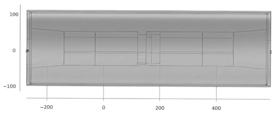
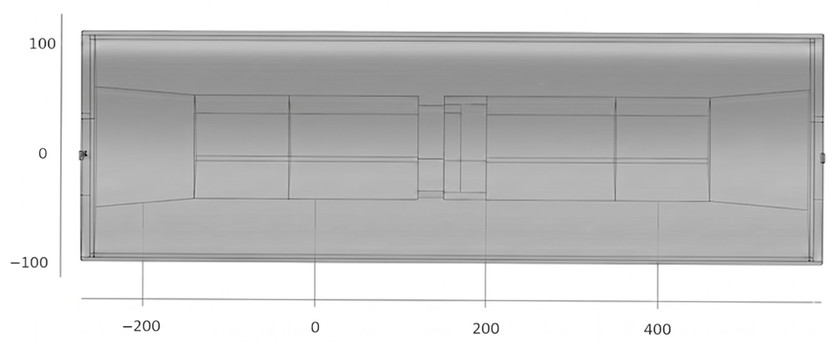
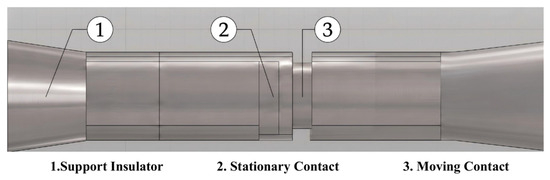
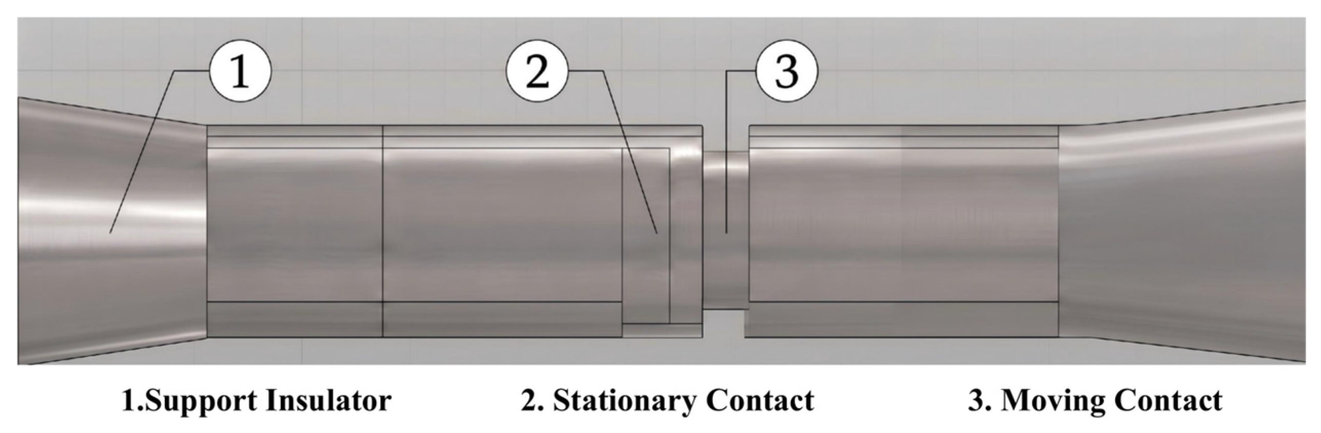
The motion of particles in practical environments involves considerable complexity. The internal GIS/GIL model established is a full-scale 3D GIS/GIL. It integrates a central conductor rod alongside a support insulator, a stationary contact, and a moving contact within a grounded metallic shell. The internal energized components are mechanically stabilized and electrically isolated from the shell by the high-performance support insulator. The 3D GIS/GIL model is shown in Figure 1 and the schematic diagram of the interior of the GIS/GIL is shown in Figure 2.

Figure 1. 3D GIS/GIL model.

Figure 2. Schematic diagram of the interior of the GIS/GIL.

3. Simulation Results

To capture the stochastic nature of particle behavior under complex electric fields, a randomized batch simulation protocol comprising 50 independent runs is executed. The initial spatial coordinates are randomly distributed at the bottom, and the initial voltage phase angles are uniformly sampled from $[0,2\pi ]$.

3.1. Simulation Analysis of Motion Characteristics

To investigate dynamic behavior under electric fields, this study introduces aluminum particles into the established simulation model, applying the 40.5 kV power-frequency voltage. The detailed configuration parameters, material properties, boundary conditions, and solver settings are summarized in Table 3.

Table 3. Key parameters and configurations for the simulation.

Category	Parameter	Value/Setting
Software and modules	Simulation software	COMSOL Multiphysics 6.3
	Coupled physics interfaces	Electrostatics Particle Tracing
Material properties	Radius of aluminum particle	0.5 mm
	Density of aluminum	2700 kg/m3
	Relative permittivity of gas	1.0
	Dynamic viscosity of gas	1.5 × 10−5 Pa·s
Boundary conditions	High-voltage conductor	40.5 kV
	shell	0 kV
Mesh and solver	Total number of elements	1,137,274
	Solver type	MUMPS
	Time step	0.1 ms

The simulation is performed by coupling an electrostatic field module with the particle tracking module: the electrostatic field is first solved to determine the spatial distribution and resulting forces acting on particles. These forces are subsequently imported as source terms into the particle tracking module to track the temporal evolution of the particle trajectory and velocity.

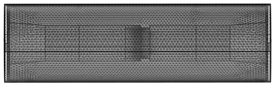
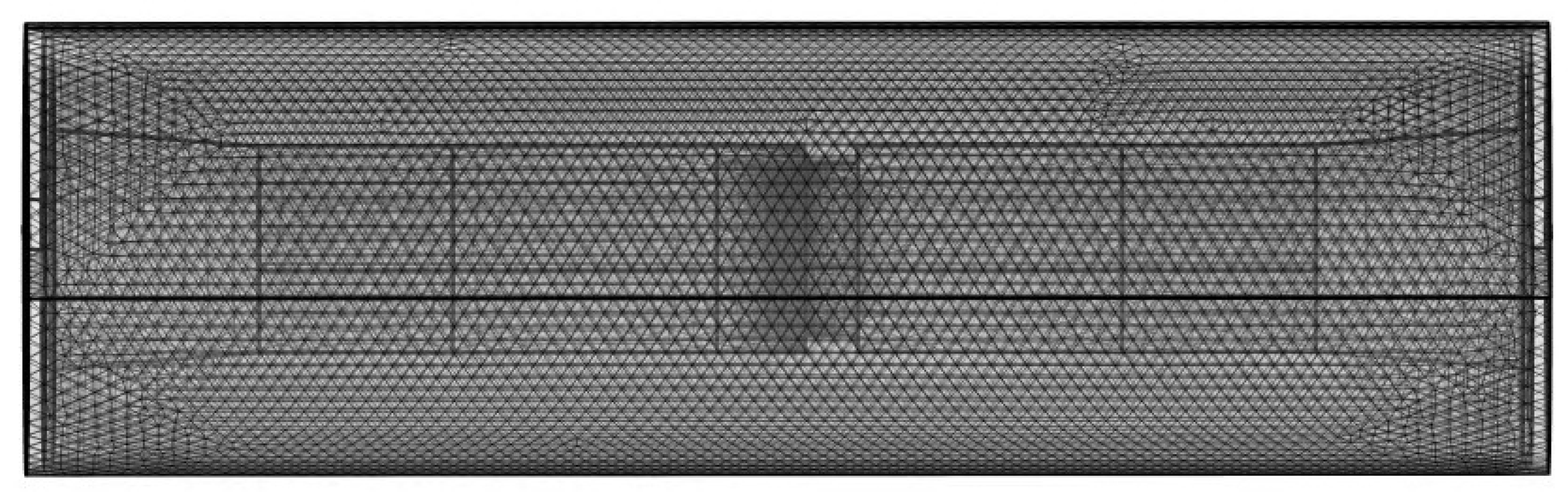
Aluminum particles of 1 mm are introduced into the established simulation model, and the power-frequency voltage of 40.5 kV is applied. The simulation is realized by coupling the electrostatic field and particle tracking module: firstly, the electrostatic field module can calculate the distribution inside GIS/GIL and the force exerted on particles, then this force is input into the particle tracking module, and finally the physical quantities such as the motion trajectory and speed of particles evolving with time are obtained. The mesh division is illustrated in Figure 3.

Figure 3. Mesh division diagram.

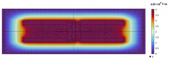
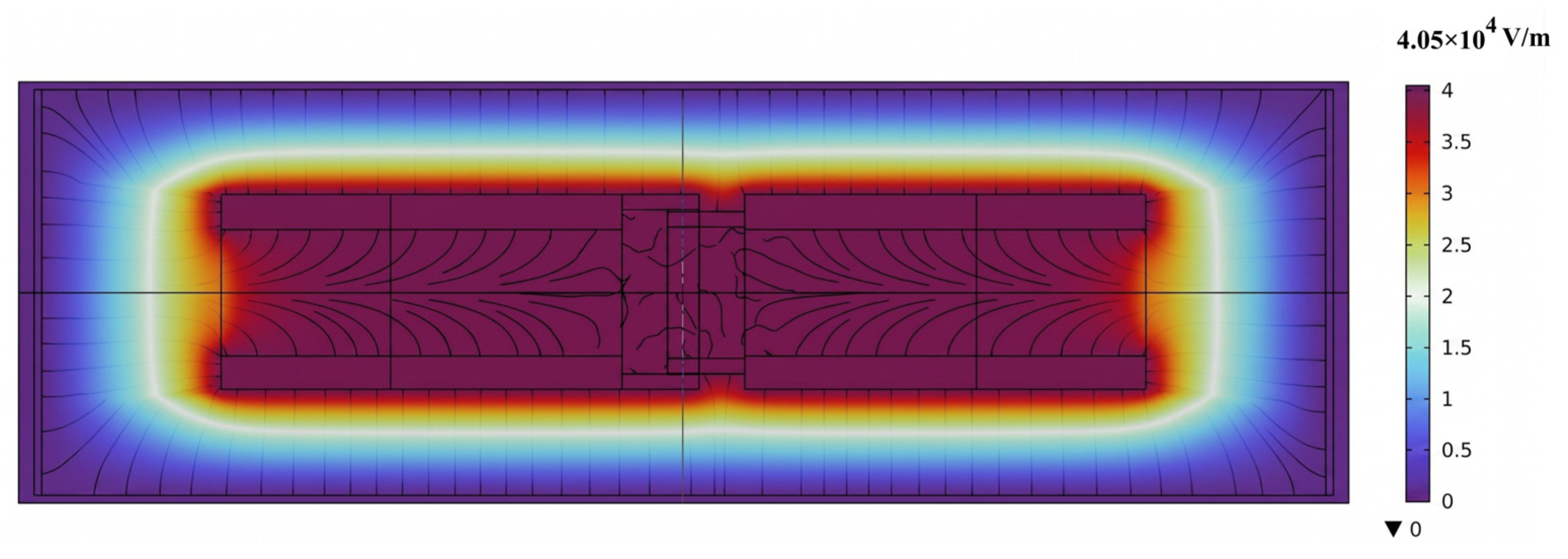
The electric field strength distribution is shown in Figure 4.

Figure 4. Electric field strength distribution diagram.

As depicted in Figure 4, the maximum electric field strength is approximately 4.05 × 10⁴ V/m. The high-intensity regions exhibit a pronounced concentration characteristic, with the peak magnitude localized at the surfaces of contacts. This distribution is physically consistent with the 3D complex geometry, where local electric field enhancement occurs at regions with a small radius of curvature and at the triple junctions of the insulator. And the field strength decreases as one moves away from the high-voltage internal components toward the grounded shell.

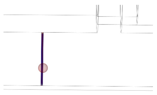
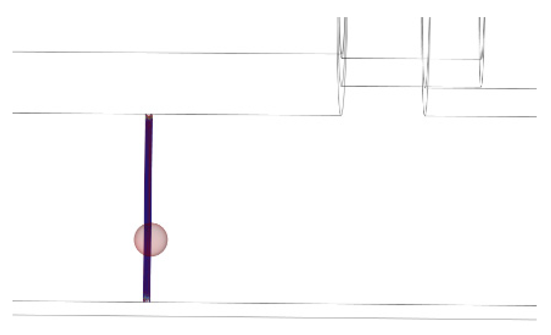
The particle trajectory is shown in Figure 5. When a high voltage is applied, particles move axially left and right after reaching the inception voltage and, meanwhile, perform continuous reciprocating motion between the chamber and the conductor rod.

Figure 5. Particle trajectory diagram.

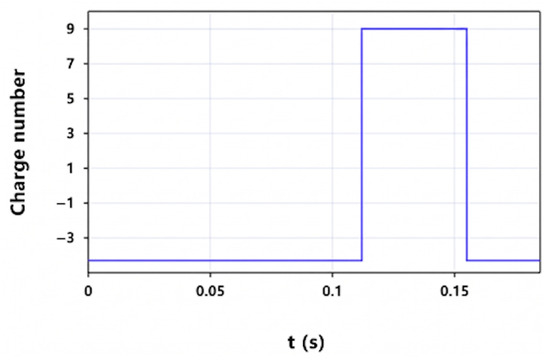
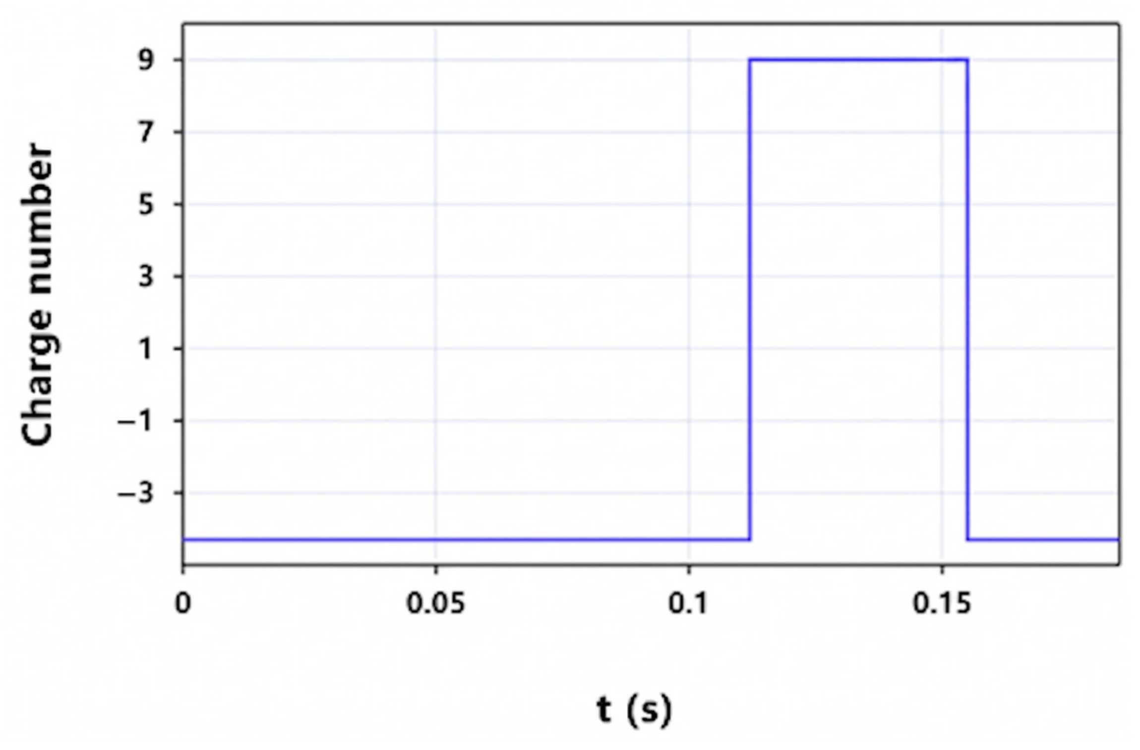
In Figure 6, Particles gradually approach the high-voltage conductor rod. After colliding with the conductor rod, the direction of the Coulomb force acting on particles tends to be consistent with that of gravity, and the charge quantity of particles increases, thus leading to their accelerated motion with decreasing acceleration until they collide with the inner surface of the grounded shell again. After this collision, the direction of the particle movement velocity reverses, the polarity of the charge carried by the particle changes from positive to negative, and the charge quantity decreases accordingly, repeating the cycle continuously.

Figure 6. Charge reversal diagram.

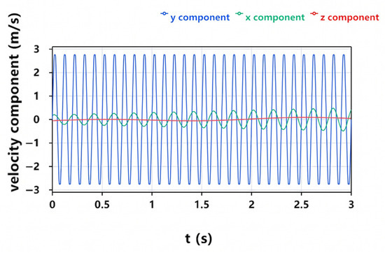
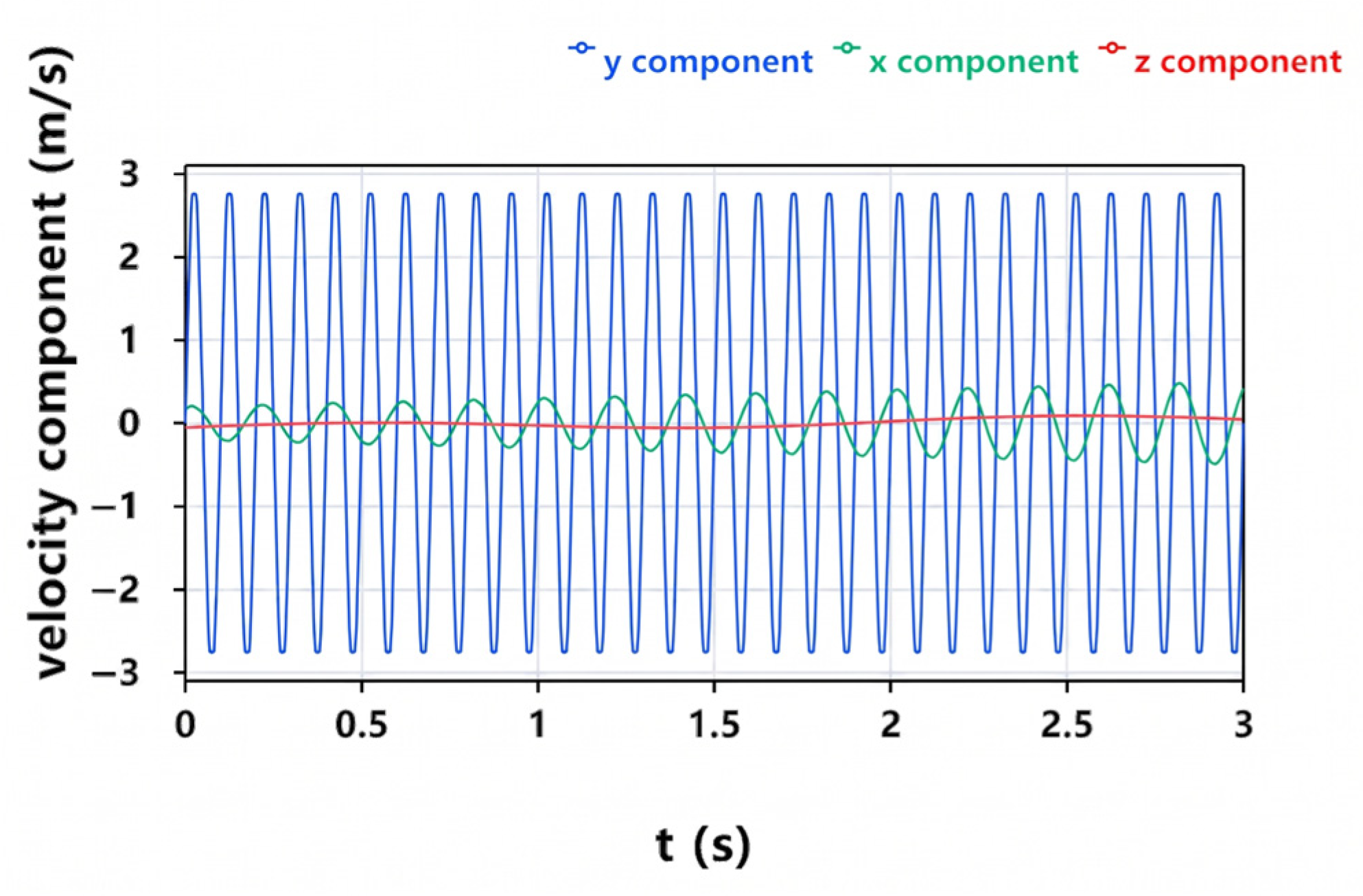
This simulation study provides an in-depth characterization of the dynamic response of metallic particles within GIS/GIL environments under a 40.5 kV power-frequency voltage. Figure 7 demonstrates that aluminum particles with a 1 mm diameter exhibit pronounced periodic reciprocating motion primarily in the vertical direction (y component), achieving a peak instantaneous velocity of 2.7 m/s. In contrast, the horizontal and axial velocity components remain relatively insignificant, indicating that the particle’s kinetic energy is highly concentrated within vertical hopping trajectories.

Figure 7. Particle velocity component diagram.

3.2. Simulation Analysis of Collision Vibration Response

Given the significant size disparity between the particles and the GIS/GIL structure, the multibody dynamic analysis primarily focuses on the transient collision dynamics at the localized contact point between the spherical particle and the chamber wall. The coupled particle motion model method, integrating the electrostatic field, particle tracking, and multibody dynamics, is employed, which computes the kinematic characteristics of the point load based on the collision response.

The collision process is simplified to the collision model between the sphere and the chamber.

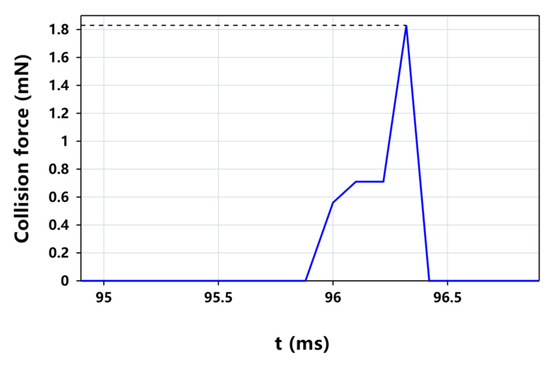
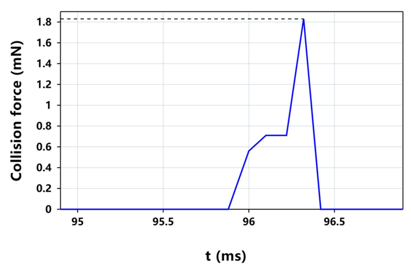
Based on the free particle motion model, the speed is obtained and assigned to particles as the initial condition. Subsequently, the point load is applied at the bottom of particles to simulate the collision force between particles and the shell, and the calculation result is shown in Figure 8. The solid blue line tracks the transient impact force, revealing a staged loading sequence that peaks at approximately 1.8 mN before rapidly dissipating. This maximum intensity is highlighted by the horizontal dashed line, which serves as a benchmark for the peak load sustained during the collision.

Figure 8. Collision force versus time diagram.

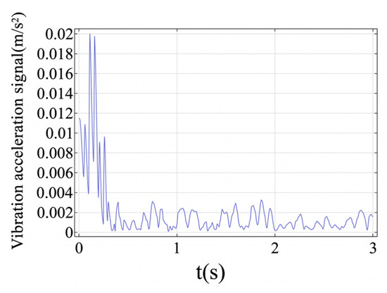
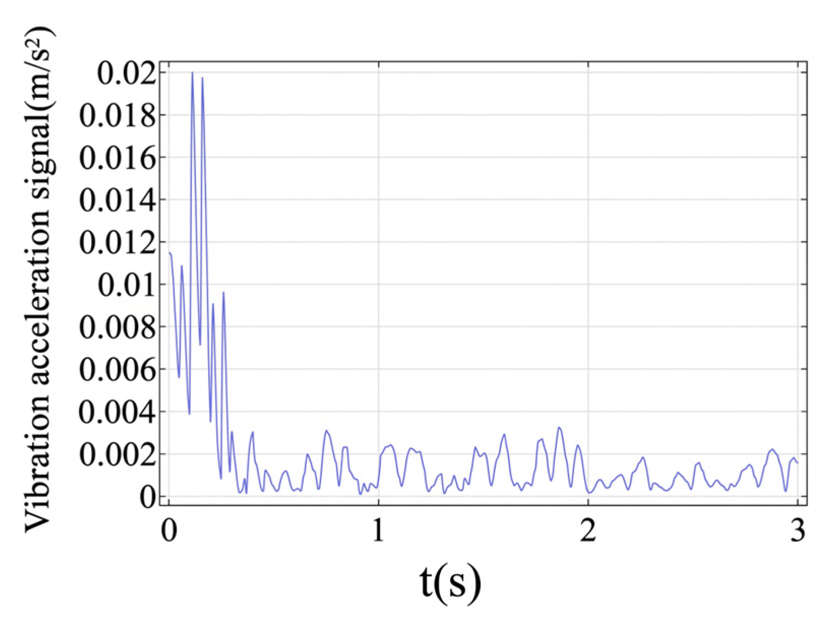
The point is selected inside the chamber to apply the collision force generated by the motion of particles as the point load, and the point outside the chamber is selected as the detection point for the acceleration signals.

The vibration acceleration signal beneath the collision point on the outer surface is shown in Figure 9.

Figure 9. Simulated vibration signal in the time domain.

Particles are released at the bottom of the chamber; due to the electric field distortion and field strength concentration at the junction of the insulator and the conductor rod, particles are attracted by this region and move toward it. The vibration signals excited by the collision of particles have significant characteristics, and the peak acceleration obtained by simulation calculation is 0.02 m/s².

3.3. Quantitative Validation and Sensitivity Analysis

3.3.1. Quantitative Validation and Statistical Analysis

To evaluate the uncertainty and variability of the particle dynamics, the statistical summaries of key simulation outputs over 50 randomized runs are presented in Table 4. The mean peak velocity of 2.70 m/s represents the average value recorded across all runs, indicating stable kinetic behavior under the designated electric field. Additionally, a sensitivity analysis on the restitution coefficient reveals that when the coefficient fluctuates between 0.6 and 0.8—accounting for potential inner wall roughness in actual equipment—the resulting collision force ranges moderately from 1.72 mN to 1.89 mN. While surface conditions introduce micro-variability, the fundamental order of magnitude of the mechanical excitation remains highly stable.

Table 4. Quantitative summary of particle collision simulation outputs (50 randomized runs).

Parameter	Mean Value	Minimum	Maximum
Peak Velocity (m/s)	2.70	2.62	2.77
Peak Collision Force (mN)	1.80	1.72	1.89

3.3.2. Sensitivity Analysis of Particle Parameters

To further understand the dynamic limitations and to justify the experimental parameter selection, a sensitivity analysis focusing on particle material and geometric dimensions is conducted.

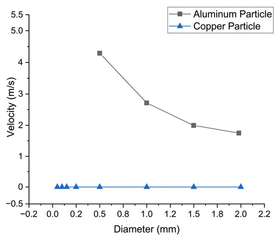
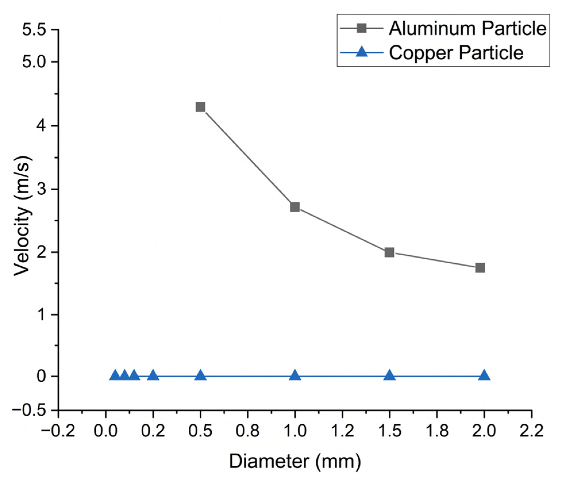
Copper possesses a density of approximately 8960 kg per cubic meter, rendering it roughly 3.3 times denser than aluminum (2700 kg per cubic meter). In Figure 10, a copper particle of a given diameter requires a significantly higher threshold voltage to accumulate sufficient charge to overcome its massive gravitational anchor. The 40.5 kV excitation voltage used in this experimental setup is simply insufficient to initiate the motion of the dense copper particles, resulting in a zero velocity reading. Analyzing the aluminum particle reveals a pronounced inverse relationship between particle diameter and maximum velocity. At a diameter of 0.5 mm, the aluminum particle approximately achieves a rapid velocity of 4.3 m per second. However, as the diameter quadruples to 2.0 mm, the velocity drops by more than half, approximately plateauing at 1.7 m per second.

Figure 10. Velocity versus particle diameter for aluminum and copper particles.

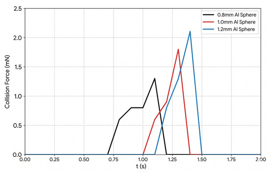
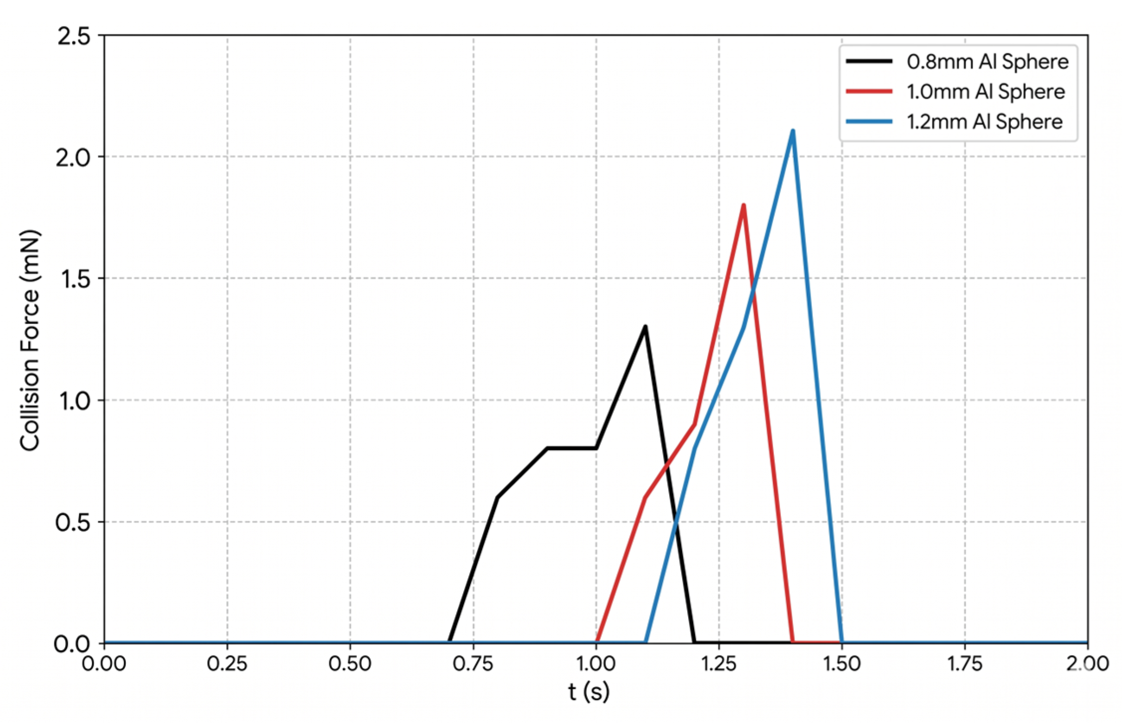
Despite the reduction in velocity, larger particles carry significantly more momentum due to their massive volume. As illustrated in Figure 11, the peak collision force exhibits a positive correlation with particle size. For instance, the 1.2 mm aluminum sphere generates a higher peak collision force compared to the 0.8 mm and 1.0 mm spheres. This analysis fundamentally validates the selection of 1.0 mm aluminum particles for the subsequent experimental stage: they are able to balance high dynamic activity (sufficient lift-off velocity).

Figure 11. Collision force over time for different sphere sizes.

3.3.3. Modal Analysis

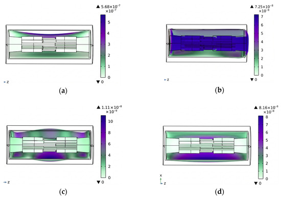
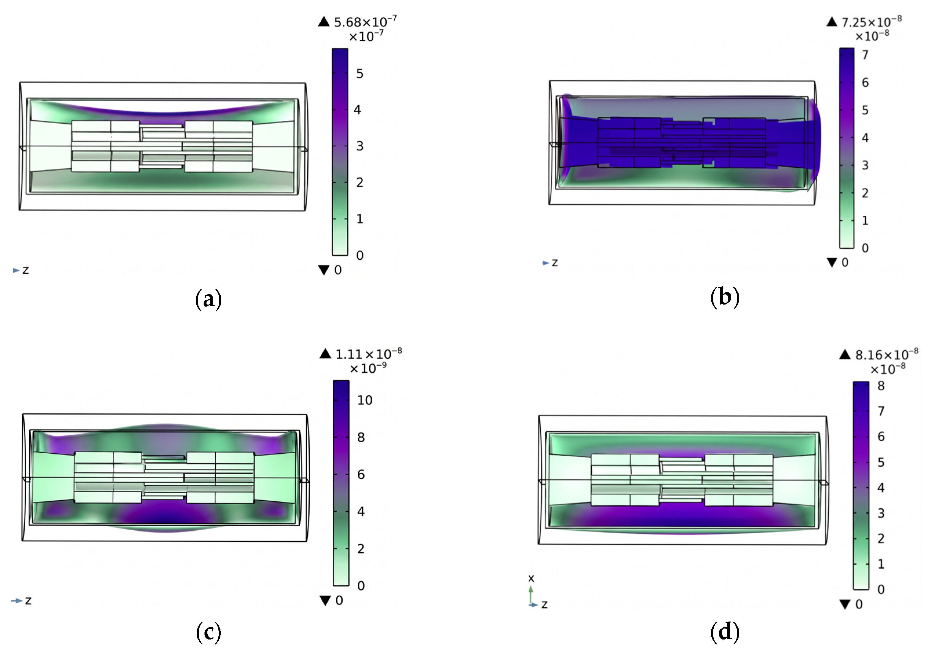
The modal analysis is conducted, and the structural resonance frequencies of the GIS/GIL structure are presented in Figure 12.

Figure 12. Natural frequency: (a) natural frequency 53.22 Hz; (b) natural frequency 231.29 Hz; (c) natural frequency 451.79 Hz; (d) natural frequency 557.37 Hz.

As illustrated in Figure 12, the natural frequencies of the GIS/GIL are all below 1000 Hz, while the frequencies induced by metallic particle collisions fall within the 1000–1500 Hz range, which inherently avoids interference from the structural resonance frequencies.

4. Construction and Analysis

4.1. Construction

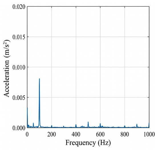
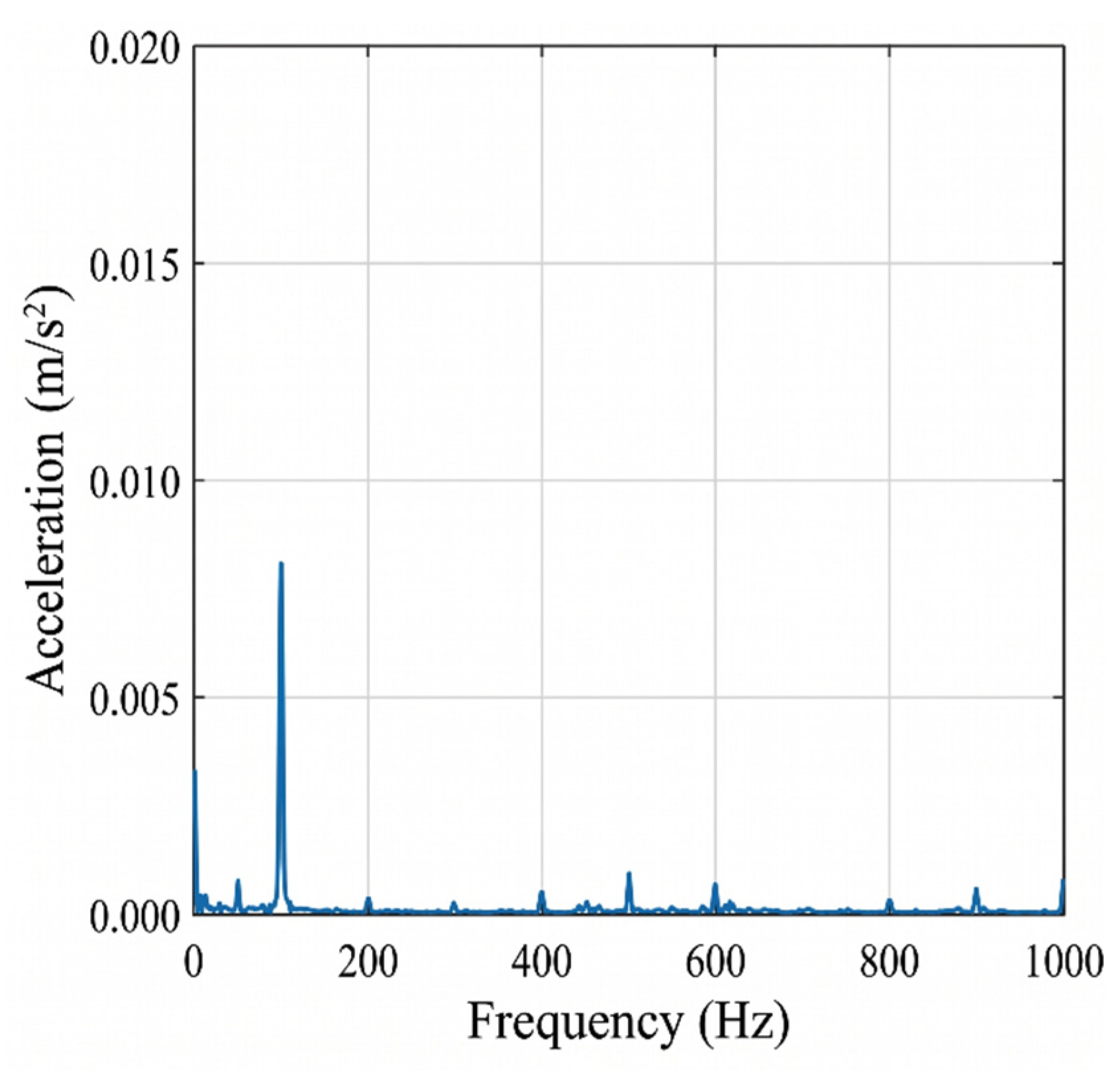
The fundamental operating frequency of GIS/GIL equipment is characterized by 100 Hz electrodynamic vibration induced by the operating current. In Figure 13, the electrical contact test, under 1000 A, is conducted.

Figure 13. Experimental result of electrical contact test.

As evidenced by the frequency spectrum, the dominant vibration source of the equipment remains at 100 Hz, whereas metallic particle collisions occur above 1000 Hz, making the two effectively distinguishable.

To ensure the full reproducibility of the experimental results, the detailed specifications of the high-voltage testing platform are comprehensively documented. The full-scale 40.5 kV prototype features a chamber length of 1500 mm, with the central high-voltage conductor and the grounded shell having radii of 40 mm and 150 mm, respectively. The chamber is pressurized with SF₆ gas at 0.4 MPa to strictly replicate actual grid insulation conditions.

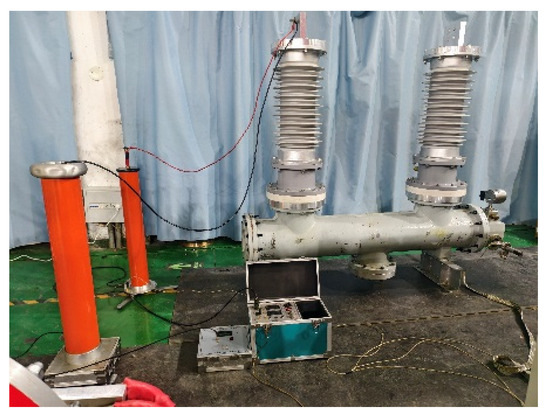
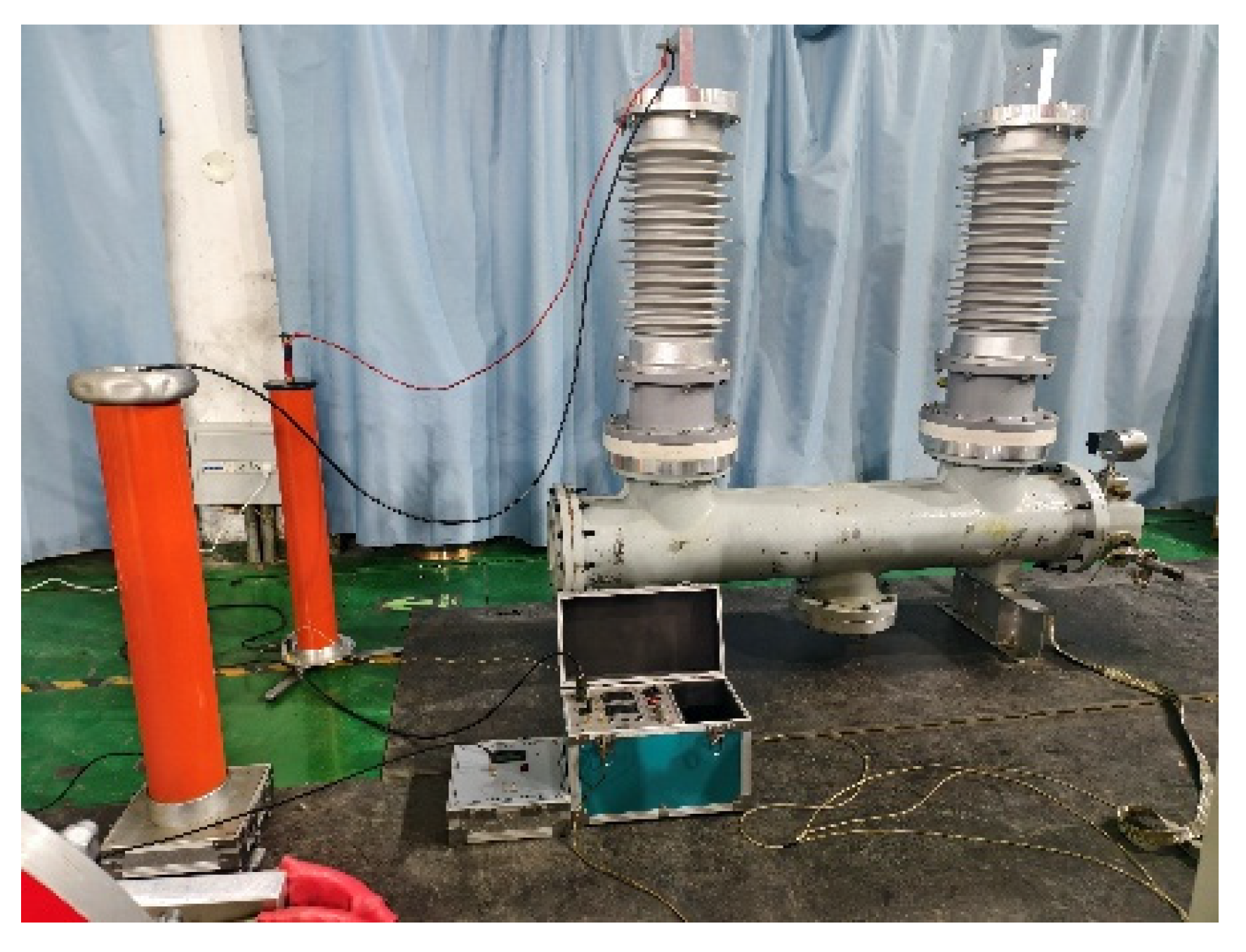
The power-supply section of the test setup includes a high-voltage generator capable of delivering the required voltage to the prototype. In addition, a voltage divider is utilized to accurately measure the applied voltage. The high-voltage experimental platform with the 40.5 kV full-scale prototype is shown in Figure 14.

Figure 14. Experimental platform with a 40.5 kV full-scale prototype.

The chamber used in the experiment is the simulated structure with the smooth inner wall, and its geometric dimensions are consistent with those of actual equipment. The aluminum particle, stationary on the inner wall of the chamber, is used as a particle simulant, which moves under the drive of the electric field.

In this experiment, the single detection point is arranged directly below the collision point on the surface of the shell. Installing a single high-sensitivity accelerometer directly beneath the predicted collision point on the grounded shell is scientifically sufficient to establish the physical mapping between particle collision dynamics and the diagnostic IMF4 component. When the particle collides with the single measurement point directly below, a distinct signal is captured. Furthermore, to accurately capture these transient features, any sensors deployed for this methodology must meet strict minimum technical requirements: a sensitivity of at least 250 mV/g to resolve micro-mechanical forces, a frequency response bandwidth of up to 5 kHz to prevent the aliasing of high-frequency transients, and robust alloy shielding to guarantee electromagnetic immunity under high-voltage excitation.

4.2. Analysis of Vibration Information Spectrum

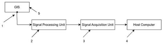
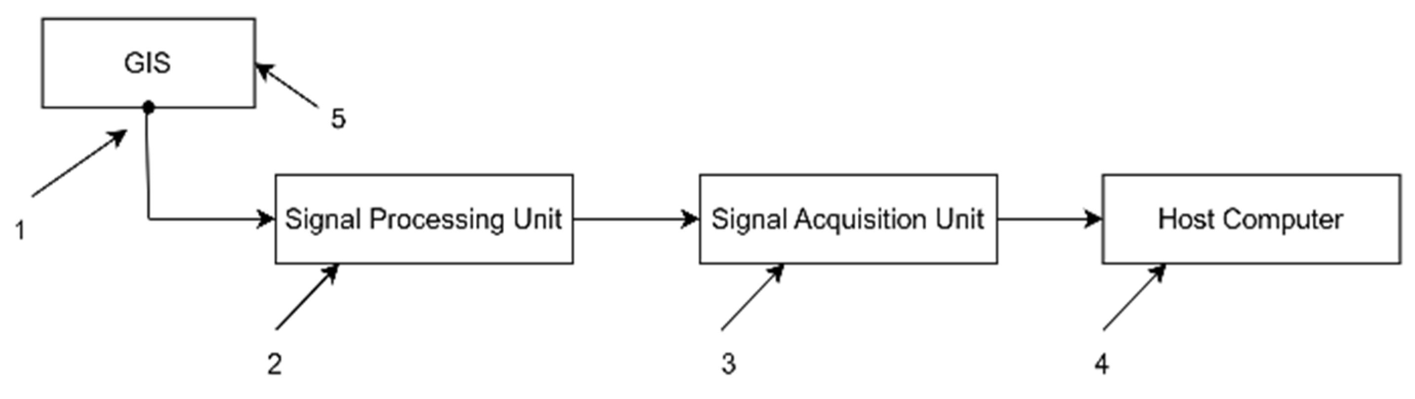
In Figure 15 and Figure 1 is the accelerometer, 2 is the signal processing unit, 3 is the signal acquisition unit, 4 is the upper computer, 5 is the shell. This figure shows the process of collecting vibration signals from the accelerometer 1 on shell 5, processing them through the signal processing unit 2, collecting them by the signal acquisition unit 3, and transmitting them to the upper computer 4 for further analysis. It is used to detect vibration signals during the operation of GIS/GIL and can assist in judging whether there are vibration defects.

Figure 15. Schematic diagram of the vibration monitoring setup.

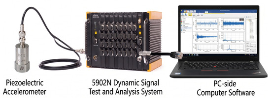
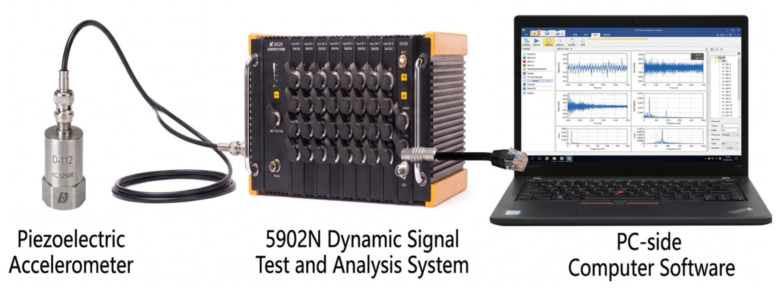
The physical configuration of the vibration monitoring platform used in this study is illustrated in Figure 16. Mechanical vibrations from the test object are captured by a DH1A941E piezoelectric accelerometer. The detailed specifications of this sensor are summarized in Table 5. To preserve the high-frequency transient characteristics of the vibration signals, the system’s sampling frequency was configured at 5 kHz, leveraging the sensor’s 250 mV/g sensitivity and ±20 g measurement range.

Figure 16. Experimental equipment for online monitoring and diagnosis system of vibration status.

Table 5. Parameters for the DH1A941E accelerometer.

Parameter	Value
Sensitivity	250 mV/g
Sampling Frequency	5 kHz
Temperature Range	−40~+120 °C
Output Connector	Side
Weight	37 g
Measuring Range	±20 g

The DH1A941E accelerometer is utilized for vibration sensing. The sensor is magnetically mounted onto the GIS/GIL shell, ensuring reliable attachment while allowing for flexible adjustment of measurement locations. The data acquisition module employs oversampling techniques to streamline system architecture and enhance measurement fidelity. It incorporates a digital linear-phase anti-aliasing filter, achieving a passband ripple of less than ±0.05 dB at 43% Fs, which provides excellent amplitude and phase-frequency responses.

To operate in complex electromagnetic environments, the acquisition hardware is housed in an alloy casing for robust magnetic shielding. Each input channel features programmable gain and filtering, ensuring compatibility with sensors across diverse measurement ranges. Data transmission between the acquisition module and the host PC is established via a Gigabit Ethernet connection, and the system is rapidly initialized by identifying the module’s IP address. Finally, a dedicated host software platform manages channel selection and parameter configuration, serving as the primary interface for real-time data logging during the laboratory measurements.

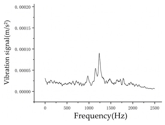
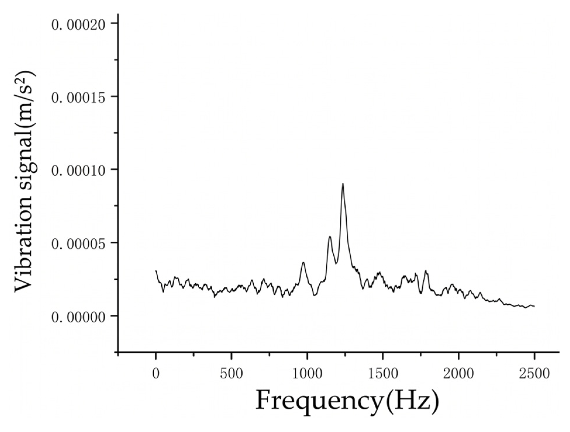
When 40.5 kV is applied to the full-scale experimental prototype, the aluminum particles lift off and collide with the chamber, generating measurable vibration acceleration signals. The signals are excited by the collision. In the time domain, the peak acceleration reflects the collision energy. In the frequency domain, it is manifested as high-frequency components.

A statistical evaluation is performed across n = 20 independent experimental runs. The key metrics—specifically the time-domain peak acceleration and the frequency-domain dominant peaks—are extracted from each trial.

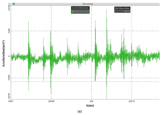
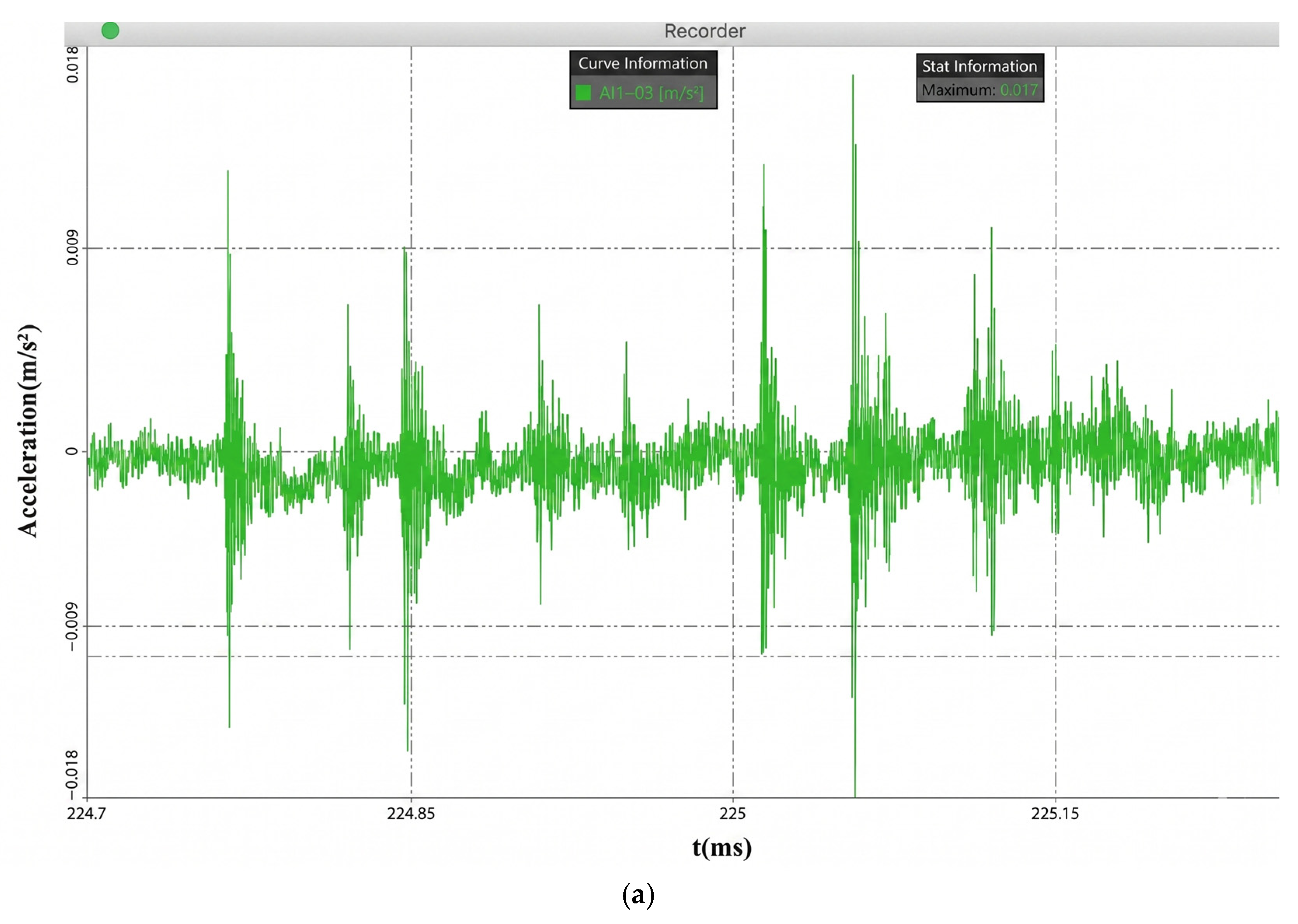
Figure 17 provides a critical morphological contrast between the active defect state and the normal operational baseline. Specifically, Figure 17a illustrates the time-domain acceleration waveform during discrete particle collisions. The collision response is characterized by an instantaneous amplitude surge. The mean peak acceleration across the 20 runs is 0.017 m/s², with a minimal margin of error. This narrow margin of error demonstrates that the mechanical energy transferred during the particle–shell collision remains highly consistent under stable grid voltages.

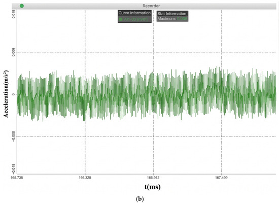
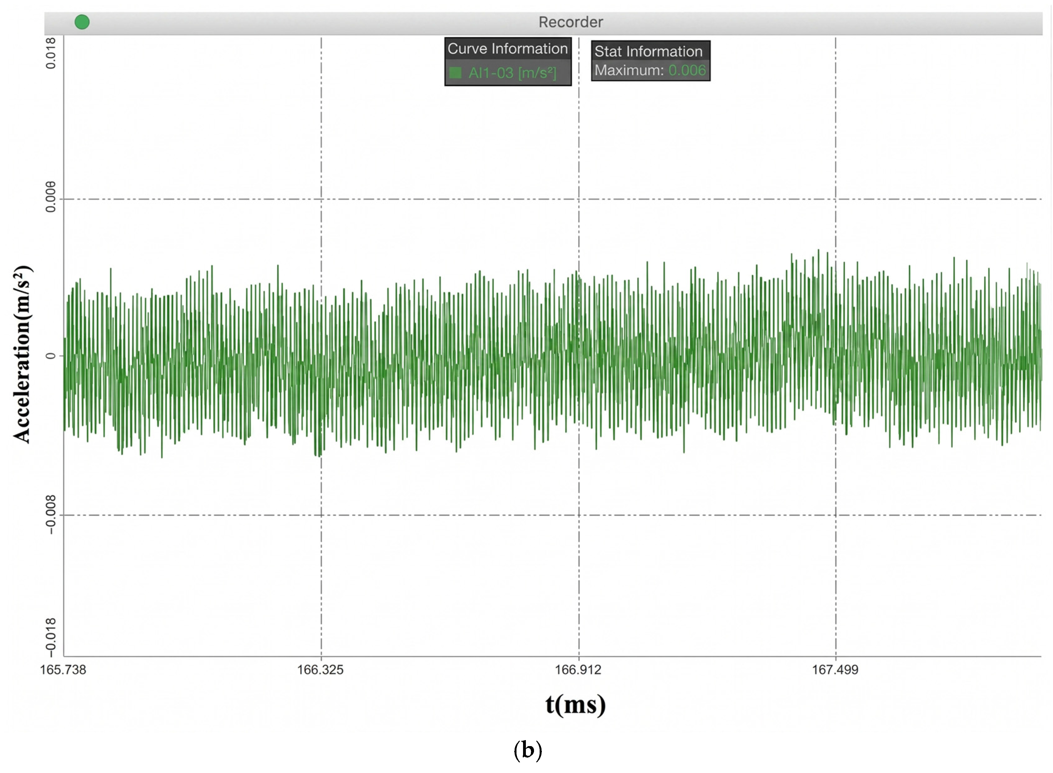
Figure 17. Time-domain vibration acceleration waveforms acquired from the full-scale prototype: (a) active particle collision state exhibiting transient impulses; (b) normal operational baseline.

Conversely, Figure 17b establishes the normal operational baseline in the absence of particle dynamics. This signal exhibits a stationary random morphology, maintaining a strictly confined maximum amplitude of 0.006 m/s².

The quantitative comparison reveals that the peak mechanical energy transferred during a particle–shell collision is nearly three times the magnitude of the normal operational baseline.

The response frequencies excited by these collisions exhibit good spectral stability. In Figure 18, the dominant high-frequency bands yield 1000–1500 Hz.

Figure 18. Vibration signals in the frequency domain.

5. Defect Diagnosis Method

Vibration signals induced by the particle’s motion have been successfully captured by the experimental platform, and the characteristic data incorporating both the time domain and frequency-domain characteristics has been constructed. The novel diagnostic methodology based on the HHT and correlation coefficient is proposed.

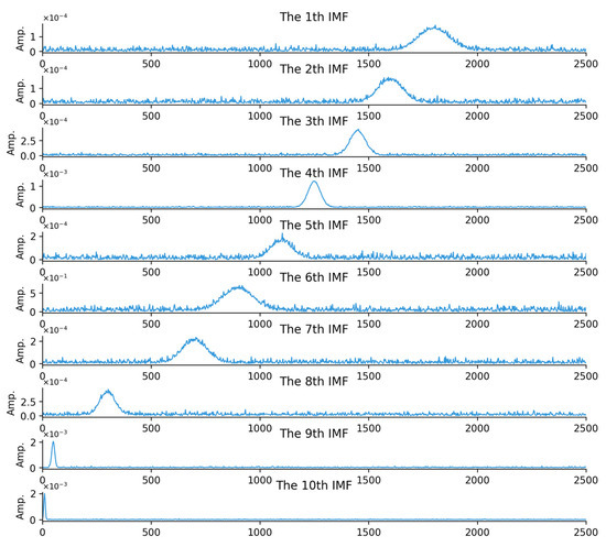
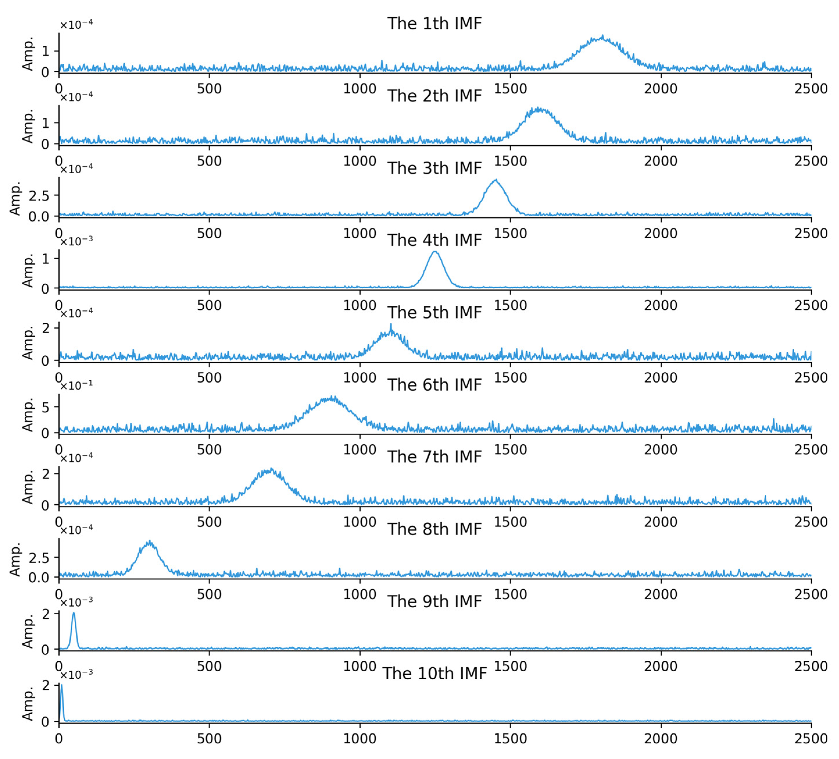
The EMD operates independently of any predefined basis functions, intrinsically isolating the IMF4. The frequency-domain analysis of both the simulation and experimental data indicates that components above 1000 Hz correspond to particle defects, the relevant components within this frequency range are extracted, and the IMF4 component is identified as the key correlation parameter reflecting the 1000 Hz frequency element.

The HHT involves two key stages: the EMD process and the application of Hilbert Transform.

EMD aims to decompose the original signal $x\left(t\right)$ into a finite set of IMFs. Each IMF must satisfy two conditions: the number of extrema and zero-crossings are either equal or differ by at most one, and the mean value of the upper and lower envelopes formed by local maxima and local minima is zero. The decomposition is carried out by first locating all local maxima and minima of $x\left(t\right)$, then performing spline interpolation through maxima and minima separately to construct the upper envelope $e_{max}\left(t\right)$ and lower envelope $e_{min}\left(t\right)$. The envelope mean is computed as:

$$m\left(t\right)={\displaystyle \frac{e_{max}\left(t\right)+e_{min}\left(t\right)}{2}}$$

(20)

Subtracting it from the original signal yields $h\left(t\right)=x\left(t\right)-m\left(t\right)$. If $h\left(t\right)$ satisfies the IMF criteria, it is taken as an IMF. Otherwise, it becomes the new target signal, and the above steps are repeated until the criteria are met. The obtained IMF is then removed from the original signal to form a residual, which is treated as the new input and decomposed in the same manner. This iterative process continues until the residual contains no meaningful IMF components. Finally, the original signal can be expressed as the sum of all IMFs and the residual:

$$x\left(t\right)={\displaystyle \sum _{i=1}^{n}IMFi(t)}+r\left(t\right)$$

(21)

$IMFi(t)$ is the i-th IMF and $r\left(t\right)$ is the residual.

After EMD, Hilbert spectral analysis is applied to each IMF to obtain instantaneous amplitude. For a given signal $s\left(t\right)$, its Hilbert transform is denoted by $\widehat{s}\left(t\right)$. An analytic signal can then be constructed as $z\left(t\right)=s\left(t\right)+j\widehat{s}\left(t\right)$.

Correlation coefficient analysis is subsequently used to quantify the linear relationship between each IMF component and the original vibration signal, so that IMFs that best reflect fault-related characteristics can be identified. Pearson correlation coefficient $r$ is adopted for this purpose, defined as:

$$\mathrm{r}={\displaystyle \frac{{\displaystyle {\sum }_{i=1}^n(x_i-\overline{x})}(y_i-\overline{y})}{\sqrt{{\displaystyle {\sum }_{i=1}^n{(x_i-\overline{x})}^2}{\displaystyle {\sum }_{i=1}^n{(y_i-\overline{y})}^2}}}}$$

(22)

$x$ denotes the ordinal index of the frequency band corresponding to the decomposed IMF, $y$ denotes the values of the IMF component, $x_i$ and $y_i$ are the i-th observations, $\overline{x}$ and $\overline{y}$ are the means of the two variables, and $n$ is the total number of samples.

The means are first computed as:

$$\overline{x}={\displaystyle \frac{1}{n}}{\displaystyle \sum x_i},\overline{y}={\displaystyle \frac{1}{n}}{\displaystyle \sum y_i}$$

(23)

Then deviations from the mean are obtained:

$$x_i-x,y_i-y$$

(24)

Followed by calculating the products of deviations and the sums of squared deviations:

$${\displaystyle {\sum }_{i=1}^n{(x_i-\overline{x})}^2}{\displaystyle {\sum }_{i=1}^n{(y_i-\overline{y})}^2}$$

(25)

The correlation coefficient is finally computed using the standard Pearson formula, with $r\in [-1,1]$.

In this study, IMFs are extracted via a computational framework implemented in MATLAB R2024b, facilitating a rigorous assessment of their respective spectral–temporal characteristics. By synthesizing these properties with a correlation-based selection criterion, the most salient IMF components are systematically identified and isolated.

Figure 19 presents the spectral amplitude distributions of the IMFs. To address the physical significance of the decomposition, the subplots for the 1st to 10th IMFs are arranged sequentially. In each subplot, the horizontal axis explicitly represents the frequency, while the vertical axis denotes the normalized signal amplitude. This spectral visualization enables a granular observation of the frequency-domain morphology; specifically, the decomposition effectively isolates the collision-induced high-frequency components, with significant energy concentration observed in the 1000 Hz and 1500 Hz bands across the IMF4 and adjacent modes.

Figure 19. Amplitude distribution diagram of the IMFs.

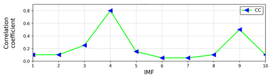
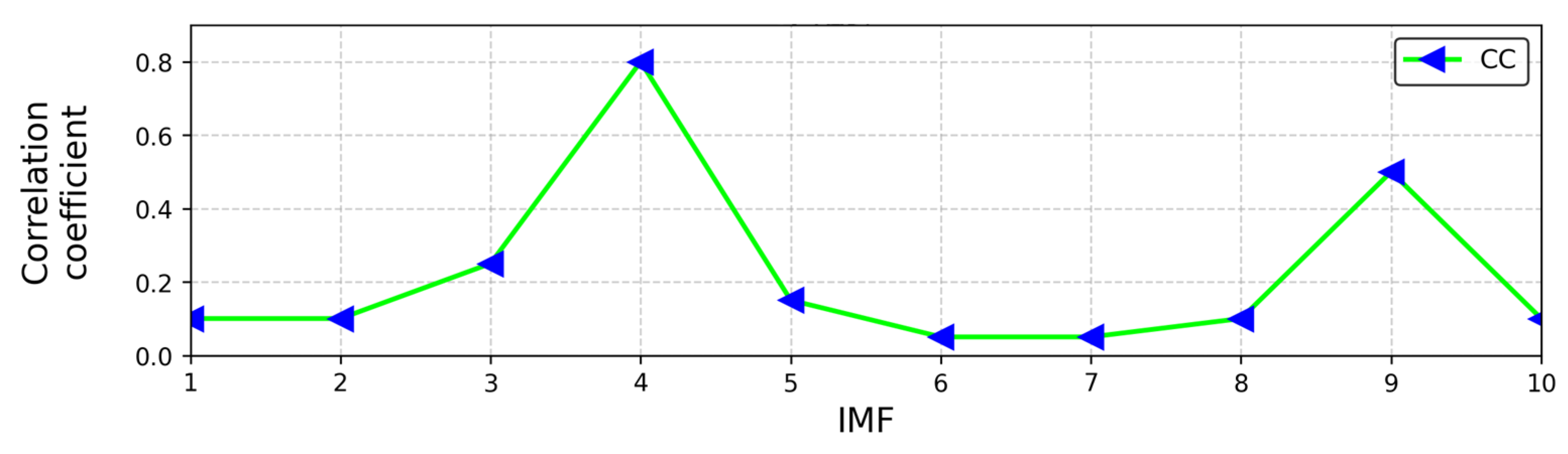
The correlation coefficient analysis is implemented. Figure 20 depicts the quantitative linear dependence between each ordinal IMF component and the raw vibration signal. The horizontal axis indicates the IMF ordinal index (1 through 10), and the vertical axis represents the calculated correlation coefficient magnitude. The data manifests a localized peak at the IMF4 component, which corresponds to the 1000 Hz characteristic band identified in the previous spectral analysis. Statistical evaluation reveals that the correlation coefficient of IMF4 consistently exceeds the diagnostic threshold of 0.7668 when metallic particle defects are present.

Figure 20. Correlation coefficient analysis diagram.

To establish the quantitative diagnostic data, this study collects vibration signals samples under the vibration state of particles. After the HHT processing, the HHT and correlation coefficient dataset and the vibration characteristic database are constructed. Statistical analysis shows that around the 1000 Hz frequency band, the correlation coefficient between the IMF4 and the original signal is significantly higher than that of other IMF components, and its value stably exceeds 0.7668, while the correlation coefficients of the other components are much lower than this threshold. The diagnostic threshold of 0.7668 is determined through a statistical analysis of the experimental database derived from n = 20 independent, repeated experimental runs on the 40.5 kV full-scale prototype.

The EMD preserves the core time–frequency features of the collision. This ensures that the diagnostic criterion remains deterministic and reliable across complex industrial environments.

Based on this law, this study proposes the following diagnostic conclusion: when the correlation coefficient between the IMF4 component and the original signal after the HHT decomposition of the vibration signals is greater than 0.7668, it can be determined that there are particle defects. This research provides an effective method for the accurate diagnosis of particle defects.

6. Discussions

6.1. Economic Feasibility and Cost–Benefit Prospect

The scalable deployment of the proposed vibration-based diagnostic methodology inevitably introduces additional hardware costs, primarily encompassing piezoelectric accelerometers, distributed data acquisition modules. From a macro-economic perspective, equipping each isolated gas compartment of GIS/GIL with a localized sensor array represents an incremental capital expenditure (CAPEX) for the condition monitoring system. However, this initial investment must be evaluated against the operational expenditure (OPEX) savings it yields. Unlike intrusive electrical detection methods (such as built-in UHF sensors) that require complex structural modifications and costly planned outages for installation, the proposed non-intrusive mechanical sensing architecture can be externally retrofitted to the grounded shell, significantly reducing deployment overhead.

More importantly, the early detection of metallic particle defects—before they initiate irreversible insulation breakdown or flashover—prevents catastrophic equipment failure. The financial avoidance of unscheduled grid outages, emergency repair costs, and subsequent revenue losses severely outweighs the deployment costs of the vibration monitoring system. To formally quantify these economic boundaries, future research will focus on conducting comprehensive life-cycle cost–benefit analyses (CBA) in operational substations.

6.2. Comparative Analysis of Existing Defect Detection Technologies

Currently, the condition monitoring of GIS/GIL equipment predominantly relies on electrical and acoustic techniques, including Ultra-High Frequency (UHF), TEV, and Ultrasonic (Acoustic Emission, AE) methods. While these technologies are mature, they present inherent limitations when detecting early-stage metallic particle defects:

• UHF Method: UHF offers exceptionally high sensitivity to partial discharge (PD) and excellent spatial localization capabilities. However, UHF sensors generally require intrusive installation (built-in sensors) or unshielded dielectric windows, leading to high retrofitting costs. More critically, UHF only detects electrical faults; it is fundamentally blind to the mechanical movement of bouncing particles before they initiate partial discharge.
• TEV Method: TEV relies on detecting high-frequency current pulses escaping the grounded shell. While strictly non-intrusive and cost-effective, TEV signals are notoriously susceptible to severe electromagnetic interference (EMI) and corona noise prevalent in high-voltage substations, leading to high false-alarm rates.
• Ultrasonic (AE) Method: AE is immune to EMI and highly sensitive to high-frequency stress waves. Nonetheless, acoustic waves suffer from extreme attenuation across the GIS/GIL shell and SF₆ gas interface, drastically limiting the effective detection range and requiring a massive number of sensors to cover a single bay.

In contrast, the implementation of the HHT-based IMF4 correlation criterion uniquely isolates the IMF4, ensuring high diagnostic reliability.

6.3. Practical Applications and Next Steps

This study investigates the vibration characteristics of metallic particles, providing a theoretical foundation for condition-based maintenance of GIS/GIL equipment and contributing to the mitigation of insulation defects induced by particles. The diagnostic technology, through ongoing collaboration with power grid enterprises, facilitates a more advanced experimental platform. Future efforts will focus on a distributed multi-sensor array and accumulating operational data across diverse working conditions, so as to promote the standardized and large-scale application of this technology.

7. Conclusions

The following conclusions are obtained:

• The mathematical model and the simulation model that can accurately reflect the motion of particles under electric field are established. The maximum electric field strength is 4.05 × 10⁴ V/m, the motion speed of aluminum particles in the chamber can reach 2.7 m/s, and the peak vibration acceleration obtained by simulation calculation is 0.02 m/s². Meanwhile, the lifting conditions, motion trajectory of particles, and the law of charge reversal, speed, and vibration changes during collision are revealed.
• The 40.5 kV GIS/GIL full-scale prototype high-voltage experimental platform is built. The power supply part of the experimental system is composed of a high-voltage generator to provide voltage for the GIS/GIL full-scale prototype, and a voltage divider is used to accurately measure the applied voltage. The vibration signals of particles are successfully detected. The result shows that when the particle motion occurs, the peak vibration acceleration is 0.017 m/s², and high-frequency components such as 1000 Hz and 1500 Hz appear. Based on this, the corresponding vibration information spectrum is constructed. Both the simulated and experimental data demonstrate close agreement within the 1000–1500 Hz frequency range, which substantiates the effectiveness of the proposed method.
• The defect diagnosis method based on the HHT and correlation coefficient analysis is proposed. The study result shows that after empirical mode decomposition of the vibration signals, the correlation coefficient between the IMF4 and the original signal at 1000 Hz is significantly larger than other components. When particle defects occur, the correlation coefficient between the IMF4 component and the original signal exceeds 0.7668.

References

- Yao, H.; Du, B.; Wang, Z.; Li, W.; Dong, J.; Liang, H. Research Progress on Functionally Graded Materials for Epoxy Insulators in HV GIL/GIS. Chin. J. Electr. Eng. 2025, 11, 150–164. [Google Scholar] [CrossRef] [Scilit]
- Jin, Z.; Du, B.; Xiao, M.; Liang, H. Dielectric Functionally Graded Materials for Control of Electric Field and Particle Motion by Topological Design and 3D Printing. Mater. Des. 2025, 257, 114517. [Google Scholar] [CrossRef] [Scilit]
- Sun, J.; Wu, N.; Fan, Y.; Lei, D.; Yang, S.; Guo, X.; Wang, H.; Song, S. Partial Discharge Characteristics of Free Moving Metal Particles in Gas Insulated Systems under DC and AC Voltages. IET Gener. Transm. Distrib. 2023, 17, 1047–1058. [Google Scholar] [CrossRef] [Scilit]
- Donzel, L.; Seeger, M.; Over, D.; Carstensen, J. Metallic Particle Motion and Breakdown at AC Voltages in CO2/O2 and SF6. Energies 2022, 15, 2804. [Google Scholar] [CrossRef] [Scilit]
- Okabe, S.; Ueta, G.; Utsumi, T. Behavior of metallic particles in GIS under DC voltage. IEEE Trans. Dielectr. Electr. Insul. 2015, 22, 2889–2897. [Google Scholar] [CrossRef] [Scilit]
- Gao, Y.; Li, Z.; Wang, H.; Yuan, X. Metal particle encouraged surface charge accumulation on epoxy insulator with multi-arc surface profile under DC voltage. IEEE Trans. Dielectr. Electr. Insul. 2020, 27, 998–1006. [Google Scholar] [CrossRef] [Scilit]
- Mier, C.; Mor, A.R.; Luo, T.; Vaessen, P. Partial Discharge and Interference Discrimination in Gas-Insulated Systems Using Electric and Magnetic Sensors. Int. J. Electr. Power Energy Syst. 2024, 158, 109911. [Google Scholar] [CrossRef] [Scilit]
- Tian, Z.; Li, X.; Sun, X.; He, J.; Xing, Y. Movement and Discharge Characteristics of Metal Dust in GIS Under AC Voltage: Focus on a Special Luminescence Phenomenon. IEEE Trans. Dielectr. Electr. Insul. 2026, 33, 723–731. [Google Scholar] [CrossRef] [Scilit]
- He, Y.; Fang, Y.; Zhang, Z.; Zhou, D.; Chen, S.; Jing, S. Partial Discharge Pattern Recognition of GIS with Time–Frequency Energy Grayscale Maps and an Improved Variational Bayesian Autoencoder. Energies 2026, 19, 127. [Google Scholar] [CrossRef] [Scilit]
- Sikorski, W.; Gielniak, J. Online Monitoring of Partial Discharges in Large Power Transformers Using Ultra-High Frequency and Acoustic Emission Methods: Case Studies. Energies 2025, 18, 1718. [Google Scholar] [CrossRef] [Scilit]
- Li, S.; Song, P.; Wei, Z.; Li, X.; Tang, Q.; Meng, Z.; Li, J.; Liu, S.; Wang, Y.; Li, J. Partial Discharge Detection and Defect Location Method in GIS Cable Terminal. Energies 2023, 16, 413. [Google Scholar] [CrossRef] [Scilit]
- Yan, J.; Wang, Y.; Zhang, W.; Wang, J.; Geng, Y.; Srinivasan, D. Domain-Alignment Multitask Learning Network for Partial Discharge Condition Assessment with Digital Twin in Gas-Insulated Switchgear. Meas. Sci. Technol. 2024, 35, 065109. [Google Scholar] [CrossRef] [Scilit]
- Duan, D.; Ma, H.; Yang, Q.; Li, N. Fault Diagnosis of Free-Conducting Particles within GIL Based on Vibration Signals. Front. Energy Res. 2023, 11, 1088549. [Google Scholar] [CrossRef] [Scilit]
- Wang, J.; Qin, C.; Zhang, T.; Chen, K.; Wu, Y.; Wang, H.; Ren, H.; Li, Q. Modelling of flaky particle motion under typical vibration excitation for gas insulated switchgear live operation. High Volt. 2025, 10, 660–672. [Google Scholar] [CrossRef] [Scilit]
- Li, X.; Hao, J.; Liao, R.; Zhong, Y.; Feng, Y.; Gong, R. Mechanical Vibration State and Its Defect Severity Development Trend Prediction for Gas-Insulated Switchgear Equipment: Attention-Bidirectional Gated Recurrent Unit Model Construction and Experimental Verification. High Volt. 2025, 10, 831–844. [Google Scholar] [CrossRef] [Scilit]
- Ma, H.; Liu, B.; Xu, H.; Chen, B.; Ju, P.; Zhang, L.; Qu, B. GIS Mechanical State Identification and Defect Diagnosis Technology Based on Self-Excited Vibration of Assembled Circuit Breaker. IET Sci. Meas. Technol. 2020, 14, 56–63. [Google Scholar] [CrossRef] [Scilit]
- Yu, Y.; Zhao, H. Research on GIS Circuit Breaker Fault Diagnosis Based on Closing Transient Vibration Signals. Machines 2025, 13, 335. [Google Scholar] [CrossRef] [Scilit]
- Duan, D.; Ma, H.; Yan, Y.; Yang, Q. A Fault Diagnosis Scheme Using Hurst Exponent for Metal Particle Faults in GIL/GIS. Sensors 2022, 22, 862. [Google Scholar] [CrossRef] [Scilit]
- Lai, Z.; Yang, M.; Li, J.; Guan, X. Internal Vibration Source Inversion of Gas Insulated Switchgear by Ensemble Kalman Filter—Finite Element Analysis and Particle Swarm Optimization. IEEE Trans. Power Deliv. 2025, 40, 3334–3344. [Google Scholar] [CrossRef] [Scilit]
- Gangsar, P.; Tiwari, R. Signal based condition monitoring techniques for fault detection and diagnosis of induction motors: A state-of-the-art review. Mech. Syst. Signal Process. 2020, 144, 106908. [Google Scholar] [CrossRef] [Scilit]
- Wang, J.; Hu, Q.; Chang, Y.; Wang, J.; Liang, R.; Tu, Y. Metal particle contamination in gas-insulated switchgears/gas-insulated transmission lines. CSEE J. Power Energy Syst. 2021, 7, 1011–1025. [Google Scholar]
Disclaimer/Publisher’s Note: The statements, opinions and data contained in all publications are solely those of the individual author(s) and contributor(s) and not of MDPI and/or the editor(s). MDPI and/or the editor(s) disclaim responsibility for any injury to people or property resulting from any ideas, methods, instructions or products referred to in the content. |
© 2026 by the authors. Licensee MDPI, Basel, Switzerland. This article is an open access article distributed under the terms and conditions of the Creative Commons Attribution (CC BY) license.