Deployment-Oriented Lithium-Ion Battery Remaining Useful Life Prediction with Adaptive History Selection and Parameter-Efficient Updating

Abstract

For battery management systems, accurate remaining useful life (RUL) prediction is important, yet models trained offline may not remain well matched to individual cells during operation, because degradation trajectories differ across cells and evolve over aging stages. This study examines a lightweight online personalization strategy under a representative convolutional neural network–long short-term memory (CNN–LSTM) online-transfer setting while keeping the backbone architecture and fixed input length unchanged. The proposed method restricts online updates to a small adaptation path and adjusts the effective history span according to recent degradation behavior. Experiments on 22 test cells under unseen protocols show that the method improves average post-adaptation RUL performance relative to the representative baseline, reducing the root mean square error (RMSE) from 186.00 to 160.58. The number of trainable parameters involved in online updating is reduced from 74,880 to 2193, while the average update time per step decreases slightly from 2.54 s to 2.29 s. Cell-level analysis further shows that the benefit is not uniform across all cells, motivating more selective updating for safer deployment. Overall, the results indicate that lightweight online personalization can improve the accuracy–cost trade-off of deployment-oriented battery prognostics.

1. Introduction

Lithium-ion batteries are now widely deployed in energy-storage and electrified systems, where safety margins, service continuity, and maintenance costs increasingly depend on accurate degradation tracking [1,2]. In such settings, battery management is concerned not only with instantaneous operating states, but also with remaining useful life and the prediction of future degradation [3,4]. Two quantities are commonly used for this purpose. Remaining useful life (RUL) refers to the number of cycles remaining before end-of-life, whereas state of health (SOH) reflects the gradual loss of available capacity during use [5]. Reliable estimation of these quantities is therefore important not only for fault prevention, but also for maintenance scheduling, service planning, and the effective utilization of battery assets [2].

Battery prognostics is complicated by heterogeneity across cells and by nonstationary degradation within each cell. Even under similar nominal operating conditions, batteries can follow different aging trajectories, and the degradation rate of a single cell may change over its lifetime [6,7]. This variability can leave a global model trained offline noticeably mismatched to a given target cell when applied directly [8,9]. Online personalization is therefore a practical requirement in real-time battery prognostics rather than an optional refinement [9,10]. Its implementation, however, is constrained by deployment conditions instead of unconstrained retraining [11,12]. Target-cell data are often scarce, particularly at early stages, so repeated parameter updates can become more vulnerable to limited data while also adding computational overhead [9,13]. The temporal context used for prediction also matters: a history span that is informative during slow aging may become less appropriate when degradation accelerates or nears a knee point [7,14]. Online battery personalization must therefore be considered not only from the perspective of prediction accuracy, but also in terms of update cost, adaptation risk, and the suitability of the temporal context.

Ma et al. [8] provide a representative online-transfer setting for studying this issue, in which a CNN–LSTM predictor is trained offline and then adapted online to each target cell under a clear and reproducible protocol. This setting makes the gap between offline generalization and cell-specific behavior explicit and provides a stable reference for comparison under comparable conditions. However, two bottlenecks remain prominent in this setting. The first concerns update burden and adaptation risk: even partial fine-tuning may still require non-negligible online computation and may increase adaptation risk when the target stream is short, noisy, or data-deficient [11,13]. The second concerns temporal-context mismatch: the fixed recent-history span used to construct the model input may not remain equally suitable across different cells or across different aging stages [7,14]. Addressing these two issues without replacing the baseline predictor is therefore of direct practical relevance.

In this work, we study a lightweight extension of the same representative online-transfer setting of Ma et al. [8] rather than proposing a new backbone architecture. The backbone architecture and the fixed input length are kept unchanged so that the comparison remains anchored to the same deployment-oriented baseline. Instead, we focus on two constrained modifications to the online procedure. First, we replace backbone fine-tuning with a parameter-efficient update path built around a small adapter and an auxiliary SOH branch, aiming to reduce update burden and limit overfitting during online personalization. Second, the fixed recent-history span is replaced with an adaptive windowing rule that adjusts the effective history span while preserving the same number of sampled input cycles. In this way, the study targets practical deployability under limited online resources rather than architectural complexity.

The aim of this study is therefore not to claim that a more complex predictor is universally superior, but to examine whether online personalization can be made less burdensome and better aligned with evolving degradation behavior under realistic deployment constraints. The key question is not only whether adaptation improves average prediction accuracy, but also whether it does so with lower update burden and fewer harmful updates. The evaluation therefore considers accuracy gain together with online update cost and adaptation risk, rather than relying on average accuracy alone. Under the same online protocol, this setting also allows cell-level variation and the interaction between RUL and SOH to be examined. The proposed design is evaluated on 22 test cells under this protocol.

Section 2 reviews the literature related to battery prognostics, online personalization, and lightweight adaptation. Section 3 presents the proposed method as a lightweight extension of a representative online transfer learning baseline. Section 4 evaluates the proposed method on 22 test cells in an online setting. Section 5 concludes the paper and outlines possible directions for future work.

2. Related Work

Existing studies relevant to this paper can be grouped into three closely related directions: battery SOH estimation and RUL prediction, personalization and transfer learning for batteries, and online learning issues associated with concept drift and lightweight adaptation. Together, these directions provide the background for the present study, whose focus is not on proposing a new backbone architecture but on improving the practicality of online battery prognostics under deployment constraints.

2.1. Battery SOH Estimation and RUL Prediction

Research on battery health prediction generally focuses on two related targets: SOH estimation and RUL prediction [5,15]. Both are important for operational safety, maintenance scheduling, and lifecycle management in electric-vehicle and energy-storage applications [2,16]. SOH describes the current health condition of a battery, typically in terms of capacity or performance loss relative to the fresh state, while RUL refers to the remaining cycles or time before a predefined end-of-life threshold is reached [5]. The two targets are closely related but serve different purposes. SOH estimation focuses on the present degradation state, whereas RUL prediction is more concerned with future degradation progression and end-of-life timing [5]. In battery management, decisions often depend on both the current health condition and the remaining usable service life.

Battery health prediction has been studied using both model-based and data-driven approaches [5,15]. Model-based and empirically motivated formulations remain appealing because they are physically interpretable and more directly connected to degradation mechanisms [2,5]. Their performance, however, can depend strongly on modeling assumptions and may degrade when the target cell population, operating conditions, or degradation patterns differ from those assumed during model construction [2,5]. Data-driven methods provide an alternative route and have been investigated extensively with the growth of public datasets and richer operational records [17,18]. These methods include conventional machine-learning pipelines based on hand-crafted features as well as deep neural networks that learn predictive representations from raw or lightly processed measurements [19,20]. Deep learning is particularly relevant in this context because battery degradation is nonlinear, history-dependent, and variable across cells and operating protocols [2,21].

Much of the literature on SOH and RUL evaluates models in offline settings, where training and testing follow fixed data partitions and deployment-time adaptation is not included in the design objective [2,9]. These settings are useful for benchmarking predictive performance, but they do not fully capture the causal and reliability requirements faced by battery-management systems as new target-cell data become available during operation [9,22]. In particular, a model that performs well on average in offline evaluation may still suffer from limited generalization when deployed on a previously unseen cell whose aging trajectory differs from that of the source population [9,23]. This limitation motivates the next line of work, namely, personalization and transfer learning for battery prognostics.

2.2. Personalization and Transfer Learning for Batteries

A major challenge in battery prediction is that degradation patterns do not transfer cleanly from one cell to another [9,23]. Even cells from the same batch may diverge over time, and differences in operating conditions or aging stage may further alter the degradation trajectory [6,7]. As a result, a model trained on one group of cells may lose accuracy when applied directly to a new target cell with a different usage pattern or health trajectory [24,25]. This gap between population-level training and cell-level deployment has made personalization and transfer learning increasingly important in battery prognostics [9,10]. Representative studies have also examined transfer-learning-based RUL prediction under cell-to-cell differences, further underscoring the importance of individual variability in battery prognostics [26].

Existing transfer-oriented studies for batteries have explored several directions, including cross-condition transfer, cross-dataset transfer, and adaptation based on limited target-cell observations [9,27]. The common idea is to first extract transferable knowledge from source cells and then adapt the model to the target cell so that prediction can better reflect cell-specific behavior [9]. In engineering practice, however, the target stream is often short and not equally informative throughout, especially in the early-life stage when only limited target data are available [13,28]. This means that adaptation should not only improve accuracy, but also remain data-efficient and stable. Otherwise, the correction introduced by transfer may itself become unreliable.

For deployment-oriented battery management, this issue is particularly important because online updating is not cost-free [11,29]. Repeated adaptation consumes computation, may introduce additional latency, and may increase adaptation risk when the target data are noisy, sparse, or insufficiently representative [13,29]. Therefore, the practical question is not simply whether target-cell adaptation is possible, but whether it can be performed with acceptable update overhead and limited adaptation risk. Battery personalization, therefore, needs to be considered under deployment constraints, with computational cost, limited target-cell data, and robustness all affecting the online updating process.

The online-transfer framework reported by Ma et al. [8] provides a clear and reproducible setting in which offline pre-training is followed by target-cell adaptation during operation. For the present study, this framework makes the gap between offline generalization and online deployment explicit and serves as a controlled baseline for examining whether online personalization can be made more efficient and stable without changing the backbone architecture. However, two issues remain insufficiently addressed in such deployment-oriented settings: first, online updating may still be computationally burdensome or sensitive to target-data quality; second, the temporal context used for prediction may not remain equally suitable as degradation evolves. These two points motivate the final topic reviewed below.

2.3. Concept Drift and Lightweight Adaptation

The temporal-context issue considered in this paper is related to the broader literature on concept drift and adaptive windowing in online learning [14,30]. A central insight from that literature is that a fixed amount of historical data is not always equally useful when the underlying data-generating process changes over time [30]. For battery degradation, such non-stationarity is plausible because the aging rate may vary across cells and across life stages, and may become more pronounced near transition regions such as accelerated aging or knee behavior [7,31]. This does not mean that battery prognostics should directly adopt generic stream-learning algorithms; rather, it suggests that the suitability of a fixed recent-history span deserves careful consideration in online battery prediction.

Battery prediction models are often constructed from a fixed number of recent cycles or windows [8,19]. Although this input design is straightforward, it assumes that the same temporal span remains informative across different cells and aging stages. That assumption may not always hold. Under relatively slow degradation, a longer effective history span can retain useful trend information, whereas during faster or more localized transitions, too much history may weaken the contribution of the most recent changes [7,14]. The issue is therefore not only how many input points are used, but also whether the effective history span represented by those points remains appropriate as degradation evolves.

Another related line of work concerns lightweight adaptation, in which only a small subset of parameters is updated while the main backbone remains fixed [32]. The general motivation is to reduce update cost while keeping most backbone parameters fixed during adaptation [32]. This idea is relevant to battery prognostics because online adaptation in battery applications often occurs under strict resource and data constraints [11,13]. A lighter update path can therefore be attractive not only for computational efficiency, but also because it may help reduce adaptation sensitivity when only a short target stream is available [13,29]. Parameter-efficient updating is well suited to deployment-oriented battery personalization when the goal is to preserve the original predictor while limiting the burden of online modification.

Collectively, these studies inform the present setting without mandating a specific algorithm. In this work, adaptive windowing serves as a restricted history-selection mechanism—selecting among three predefined spans while maintaining the fixed 10-cycle input width of the representative benchmark [8]—rather than functioning as a general concept-drift detector. The parameter-efficient component likewise operates as a controlled substitute for online LSTM fine-tuning within an identical experimental setup, rather than constituting a general PEFT framework. This design enables an assessment of whether update burden and temporal-context mismatch can be mitigated within a consistent deployment-oriented baseline, motivating the method described in Section 3 without claiming universal applicability.

3. Method

This section describes the proposed method under the representative online-transfer setting introduced above. To keep the formulation relevant to deployment-oriented battery prognostics, we first define the causal online prediction setup, then describe the baseline, and finally present the two constrained strategies considered in this work: parameter-efficient updating and adaptive history selection.

3.1. Problem Setup

For each cell, the data arrive as a time-ordered sequence of charge–discharge cycles. At online step t, the predictor receives an input constructed only from information available up to that step and produces updated estimates of the target health variables under a strictly causal protocol. The exact rule used to construct the input sequence is described later, together with the baseline and the adaptive history-selection mechanism.

The model predicts two quantities simultaneously: RUL and a capacity-based SOH proxy, represented here by discharge capacity (mAh).

Formally, let $f(·;\theta )$ denote the predictor. Given the sampled input $x_t$ at step t, the model outputs ${\widehat{y}}_t^{\mathrm{rul}}$ and ${\widehat{y}}_t^{\mathrm{soh}}$, which correspond to the predicted RUL and capacity, respectively. As noted above, both prediction and adaptation at step t use only observations available up to that step.

3.2. Backbone Model and Baseline Setting

As the baseline, we use the same backbone architecture adopted in the representative online transfer learning framework [8]: a CNN–LSTM predictor with two output heads for RUL and SOH, where SOH is represented by capacity. For online battery prognostics under deployment constraints, the input size is fixed: the model [8] always takes 10 sampled recent cycles as input in this work. This setting ensures a fair comparison because all methods use the same input length and the same backbone structure.

Under the representative baseline, the model always receives 10 sampled cycles constructed from a fixed recent-history span, and online adaptation updates only the LSTM parameters while the CNN and prediction heads remain frozen [8]. This baseline is retained here as the reference setting. The two modifications examined in this work are introduced separately in Section 3.3 and Section 3.4.

3.3. Parameter-Efficient Online Personalization

Online fine-tuning can be costly and unstable when only limited target data are available, which is a practical concern for deployment-oriented battery management. To reduce the online update cost and improve stability, we freeze the CNN–LSTM backbone and update only a small set of parameters during online personalization. We achieve this by introducing a lightweight adapter module into the network. The adapter is placed after the LSTM encoder and before the prediction heads, allowing it to adjust the shared latent representation with only a small number of additional parameters. Given the latent feature vector $\mathbf{h}$, the adapter outputs an updated feature vector ${\mathbf{h}}^{\prime }$ as

$${\mathbf{h}}^{\prime }=\mathbf{h}+W_{up}\sigma \left(W_{down}\mathbf{h}\right),$$

(1)

where $W_{down}\in {\mathbb{R}}^{d_a\times d}$ and $W_{up}\in {\mathbb{R}}^{d\times d_a}$, with $d_a\ll d$, and $\sigma \left(·\right)$ is a nonlinear activation function. Here, d denotes the feature dimension (hidden size) of the LSTM output, and $d_a$ denotes the adapter bottleneck dimension.

During online adaptation on a target cell, we use the objective

$$\mathcal{L}=\lambda {\mathcal{L}}_{rul}+{\mathcal{L}}_{soh},$$

(2)

where ${\mathcal{L}}_{soh}$ denotes the capacity/SOH loss over the sampled sequence. In the reported online-update setting, $\lambda =0$. Accordingly, only the adapter and the auxiliary SOH head are updated through the weighted SOH/capacity path, while the backbone and the RUL head remain fixed. Online optimization is therefore restricted to a small set of parameters, which helps limit update cost and reduce the risk of overfitting when target-cell data are limited.

For the reported experiments, the adapter bottleneck dimension was set to $d_a=16$. The adapter used a GELU nonlinearity and no additional dropout. To keep the online update close to an identity mapping at initialization, the adapter up-projection was zero-initialized, and no additional custom initialization was applied to the remaining adapter layers. During online adaptation, only the adapter parameters and the SOH head were updated; the CNN–LSTM backbone and the RUL head remained frozen. The online optimizer was Adam with a learning rate of ${10}^{-4}$, and no additional weight decay was used. In the reported online-update setting, $\lambda$ in Equation (2) was set to 0, so the update was driven by the auxiliary capacity/SOH path, while any RUL change arose indirectly through the shared representation.

3.4. Adaptive Temporal Windowing

A fixed history window may not be equally suitable for different degradation rates in online battery prognostics. If degradation is fast, a long history may include outdated information and make adaptation less responsive; if degradation is slow, relying only on a short history may introduce noise. We therefore adopt an adaptive temporal window while keeping the model input length fixed.

The mechanism consists of two steps. At each online step, the method first determines the amount of recent history to use, denoted by $W_t$, and then converts that history into a fixed-length input through strided sampling, so that the model still receives $T=10$ sampled cycles. In the present implementation, three candidate spans, $\{10,20,30\}$, are used, corresponding to strides $\{1,2,3\}$. To select among them without relying on the model’s own predictions, the recent degradation rate is estimated from measured capacity changes. We then choose a sampling stride:

$$s_t=\left\{\begin{array}{cc}1,\hfill & g_t\ge {\tau }_{high}\left(\mathrm{fast}\mathrm{degradation}\right)\hfill \\ 2,\hfill & {\tau }_{low}\le g_t<{\tau }_{high}\hfill \\ 3,\hfill & g_t<{\tau }_{low}\left(\mathrm{slow}\mathrm{degradation}\right)\hfill \end{array}\right.$$

(3)

The most recent $W_t$ cycles are then selected, and every $s_t$-th cycle is sampled, so that the model always receives exactly $T=10$ input cycles. Faster degradation leads to denser sampling of recent history, whereas slower degradation corresponds to a longer effective history span under the same fixed-input requirement.

In the reported implementation, the degradation-rate proxy $g_t$ was computed from measured capacity only as the mean absolute cycle-to-cycle capacity change over the most recent up-to-five differences. The switching thresholds in Equation (3) were not treated as universal electrochemical constants. Instead, ${\tau }_{\mathrm{low}}$ and ${\tau }_{\mathrm{high}}$ were recomputed for each target-cell trajectory from the lower and upper terciles of the corresponding valid $g_t$ sequence in the adaptive-window generator. Across the 22 reported test cells, ${\tau }_{\mathrm{low}}$ ranged from approximately 0.1233 to 0.1872, and ${\tau }_{\mathrm{high}}$ ranged from approximately 0.1296 to 0.2625. The adaptive-window mechanism is therefore used here as a lightweight empirical discretization of recent degradation speed rather than as a direct knee-point detector.

3.5. Overall Workflow of the Proposed Online Personalization Framework

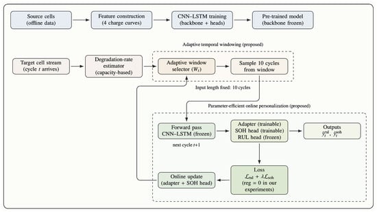
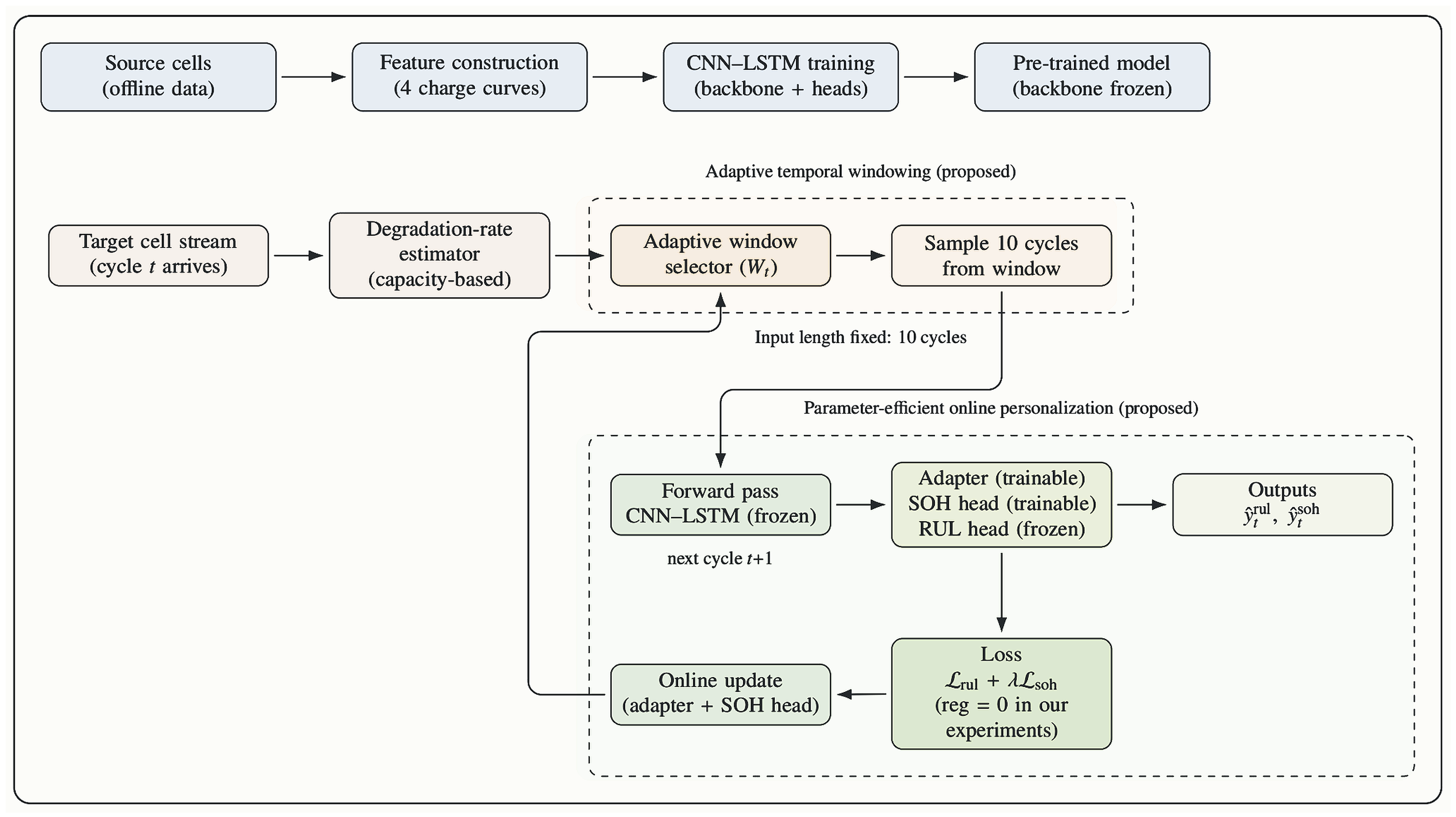
Figure 1 shows the PEAT workflow under the representative online-transfer setting. The method operates in an offline stage followed by an online stage. Offline, a CNN–LSTM predictor is trained on source cells and then reused for all target cells. Online, the input is constructed from a fixed number of sampled cycles, while the effective history span is adjusted according to recent target-cell behavior. The frozen backbone generates the predictions, and only the lightweight adaptation path is updated. The figure summarizes the workflow corresponding to the design choices described in Section 3.1, Section 3.2, Section 3.3 and Section 3.4.

Figure 1. Overview of the proposed online personalization framework based on a representative online transfer learning baseline.

4. Experiments and Results

PEAT is evaluated on 22 test cells under the same online setting as the representative baseline [8]. The evaluation examines average performance after online adaptation, the associated online update cost, and the effect of per-cell variation together with conservative safeguards on practical deployment.

4.1. Dataset and Setup

We use the same dataset and train–test split as the representative baseline study [8]. It contains degradation trajectories from 77 lithium-ion cells cycled under 77 different multi-stage discharge protocols, while the fast-charging protocol and ambient temperature are kept constant. Following the standard split used in the dataset, 55 cells are used as source cells for offline training, and the remaining 22 cells, which follow unseen discharge protocols, are used as test cells for online evaluation. For each test cell, end-of-life is defined by a capacity threshold, and the RUL target is the number of cycles remaining until that point.

We evaluate these 22 test cells in an online setting. For each cell, we first use a pre-trained CNN–LSTM model to predict RUL and SOH, and then perform online adaptation on the same cell using only the data observed up to that point. We denote the results as Before (without online adaptation) and After (with online adaptation).

To ensure a fair comparison, all methods use the same backbone, the same fixed input length of 10 sampled cycles, and the same training schedule. The comparison differs only in two experimental factors: the online update rule and the way recent history is selected to construct the 10-cycle input. Their detailed definitions have already been provided in Section 3 and are not repeated here.

Four experimental groups are considered under the same online setting: the representative baseline, the full PEAT method, and two component variants in which one of the two constrained design choices is removed. The purpose is not to claim broad generalization across multiple frameworks but to compare how different update and history-selection policies affect online personalization for battery prognostics under the same backbone and fixed-input setting.

• Baseline: fixed history span $W=30$ with stride $s=3$ (30 cycles → 10 sampled cycles); online fine-tuning updates only the LSTM parameters while keeping the CNN and prediction heads frozen (74,880 trainable parameters) [8].
• PEAT (full): adaptive temporal windowing with candidate spans $\{10,20,30\}$ (strides $\{1,2,3\}$); parameter-efficient online adaptation updates only the adapter and SOH head while keeping the backbone and RUL head frozen (2193 trainable parameters).
• PEAT without adaptive windowing (A-only): fixed history span $W=30$ and $s=3$; online adaptation updates only the adapter and SOH head (2193 trainable parameters).
• PEAT without parameter-efficient adaptation (B-only): adaptive temporal windowing with candidate spans $\{10,20,30\}$; Ma-style online fine-tuning updates only the LSTM parameters (74,880 trainable parameters).

The full PEAT setting combines both design choices, whereas the last two groups each remove one of them for ablation comparison.

For reproducibility, the main offline pretraining stage used Adam with a learning rate of $8\times {10}^{-4}$, a maximum of 10,000 epochs, early-stopping patience of 1200, mini-batch size 256, and seed 0. The online PEAT adaptation stage used Adam with a learning rate of ${10}^{-4}$, a maximum of 120 epochs, patience of 1000, and seed 2021. During online evaluation, the test stream was processed with batch size 20, except when a batch size of 21 was used to avoid a one-sample tail. The conservative Robust PEAT variant used the same optimizer with a maximum of 60 epochs and a patience of 10 for each triggered update. The implementation used deterministic seed control through fixed random seeds with CuDNN benchmark disabled and deterministic mode enabled. The provided implementation was developed under Python 3.8.8 and PyTorch 1.8.0 on Ubuntu 18.04 with a single NVIDIA RTX 3090 GPU (24 GB).

4.2. Metrics

For RUL prediction, we adopt the root mean square error (RMSE), coefficient of determination ($R^2$), and mean absolute percentage error (MAPE). RMSE quantifies the average magnitude of prediction errors in the same unit as RUL (i.e., number of cycles), with smaller values indicating better predictive performance. $R^2$ evaluates the goodness of fit between the predicted curves and the ground-truth trends, with higher values indicating better agreement between the predictions and the experimental observations. MAPE is reported as a percentage and is calculated using the same normalization protocol as in the baseline setting [8]: the absolute prediction error is normalized by a cell-level scalar (i.e., the cycle life corresponding to RUL), thereby ensuring the stability of the metric even when the RUL becomes small near battery end-of-life.

SOH estimation is evaluated using the same three metrics, namely RMSE, $R^2$, and MAPE. For MAPE, the absolute capacity-estimation error is normalized by a cell-level scalar, specifically the initial nominal capacity of the battery cell, and is then reported as a percentage.

4.3. Experimental Results for RUL

Table 1 reports the mean RUL results for the 22 test cells. For PEAT, both the pre-update results (Before) and the post-update results (After) are reported under the same evaluation pipeline. For the representative baseline, the original reference reports only the post-update results under its Task-A protocol [8]. We therefore use the published baseline After values as the external reference in Table 1, while reporting the Before/After comparison only for PEAT.

Table 1. Comparison of RUL results over 22 test protocols/cells. Baseline After values are from [8]; the corresponding Before results are not reported there.

Method	Before			After
	RMSE ↓	${\mathit{R}}^{\mathbf{2}}\uparrow$	MAPE (%) ↓	RMSE ↓	${\mathit{R}}^{\mathbf{2}}\uparrow$	MAPE (%) ↓
Ma et al. (2022) baseline [8]	–	–	–	186.00	0.804	8.72
PEAT (Full)	168.10	0.8451	8.22	160.58	0.8588	7.69

↓ : lower is better; ↑ : higher is better.

Accordingly, Table 1 compares the published post-adaptation baseline against PEAT results obtained under the same experimental conditions; it does not constitute a within-study Before/After comparison for the baseline method. Under this controlled setting, PEAT achieves better average RUL metrics after online adaptation than the representative baseline. This comparison should be read together with the efficiency analysis in Section 4.5, because deployment depends not only on average error but also on the update cost required to obtain that gain. The baseline values retained in Table 1 and Table 2 are therefore used only as published external references and not as re-estimated within-paper controls; accordingly, the magnitude of adaptation gain is interpreted within PEAT itself and is not compared across methods using Table 1.

Table 2. Component study of RUL results (After only, mean over 22 test protocols/cells). The baseline values are quoted from [8].

Method	RMSE ↓	${\mathit{R}}^2\uparrow$	MAPE (%) ↓
Ma et al. (2022) baseline [8]	186.00	0.804	8.72
PEAT without adaptive windowing	168.26	0.8556	8.05
PEAT without parameter-efficient personalization	169.30	0.8472	8.07
PEAT (Full)	160.58	0.8588	7.69

↓ : lower is better; ↑ : higher is better.

4.4. Component Study and Complementary Roles

To examine how the two design choices relate to the two deployment bottlenecks identified earlier, we compare PEAT with variants in which one component is removed at a time. Table 2 reports the mean RUL results after online adaptation. Removing adaptive windowing increases the average RMSE to 168.26, while replacing the adapter-based update with Ma-style LSTM updating increases it to 169.30. The full method achieves the best mean RMSE and $R^2$ among the tested variants, but the more important point for deployment-oriented battery prognostics is that neither design choice alone is sufficient in the current setting.

This pattern is consistent with the roles of the two components. Adaptive windowing mainly addresses temporal-context mismatch by allowing the sampled history to track the recent degradation rate, whereas parameter-efficient adaptation mainly addresses update cost and update risk by limiting the number of trainable parameters used during online adaptation. When only one of these design choices is retained, the remaining bottleneck may still weaken online personalization for part of the test set. The full method should therefore be interpreted less as a claim of synergy and more as evidence that these two deployment bottlenecks are coupled in practice: a lighter update path is more effective when the input context is better matched, and a better-matched context is more useful when the update itself remains controlled.

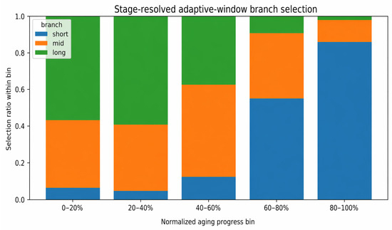
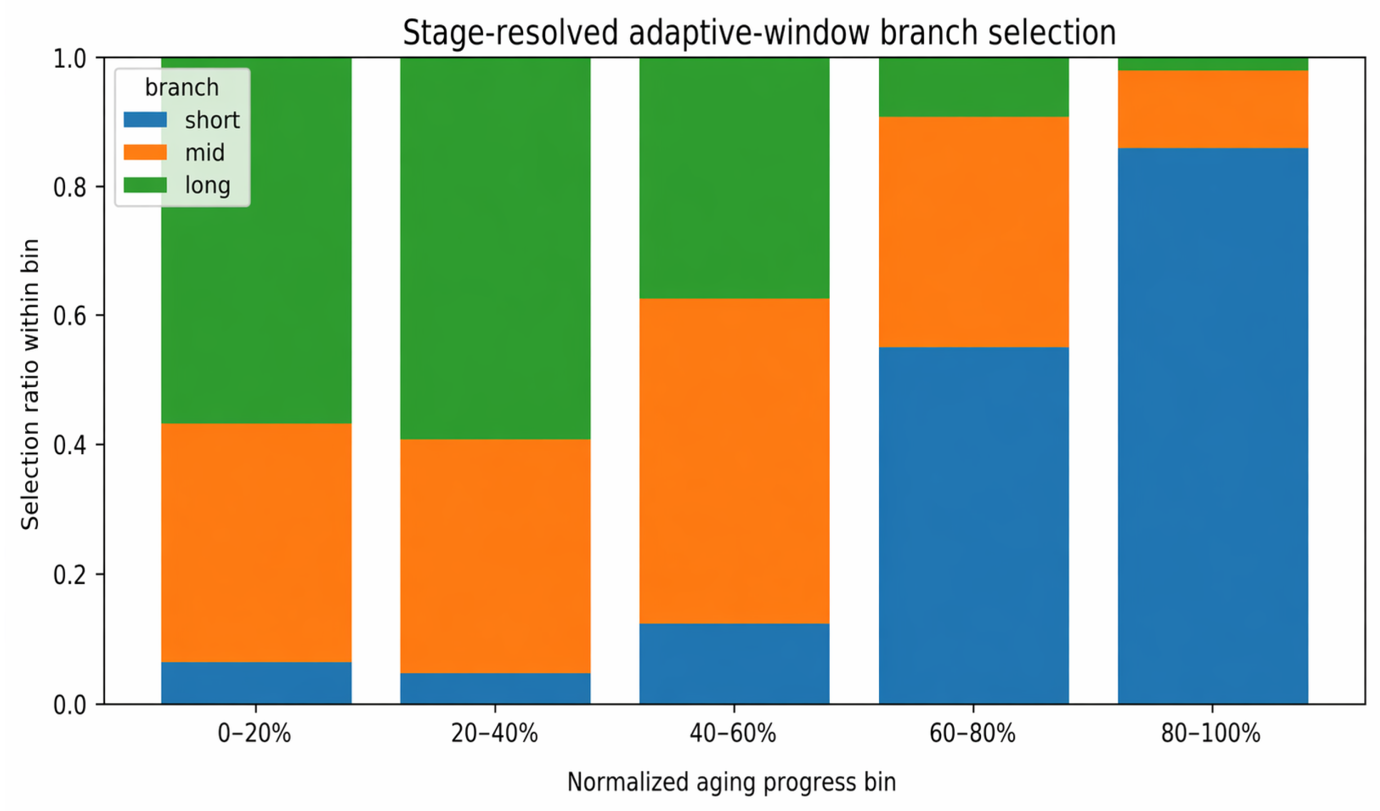
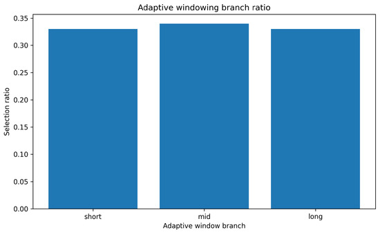
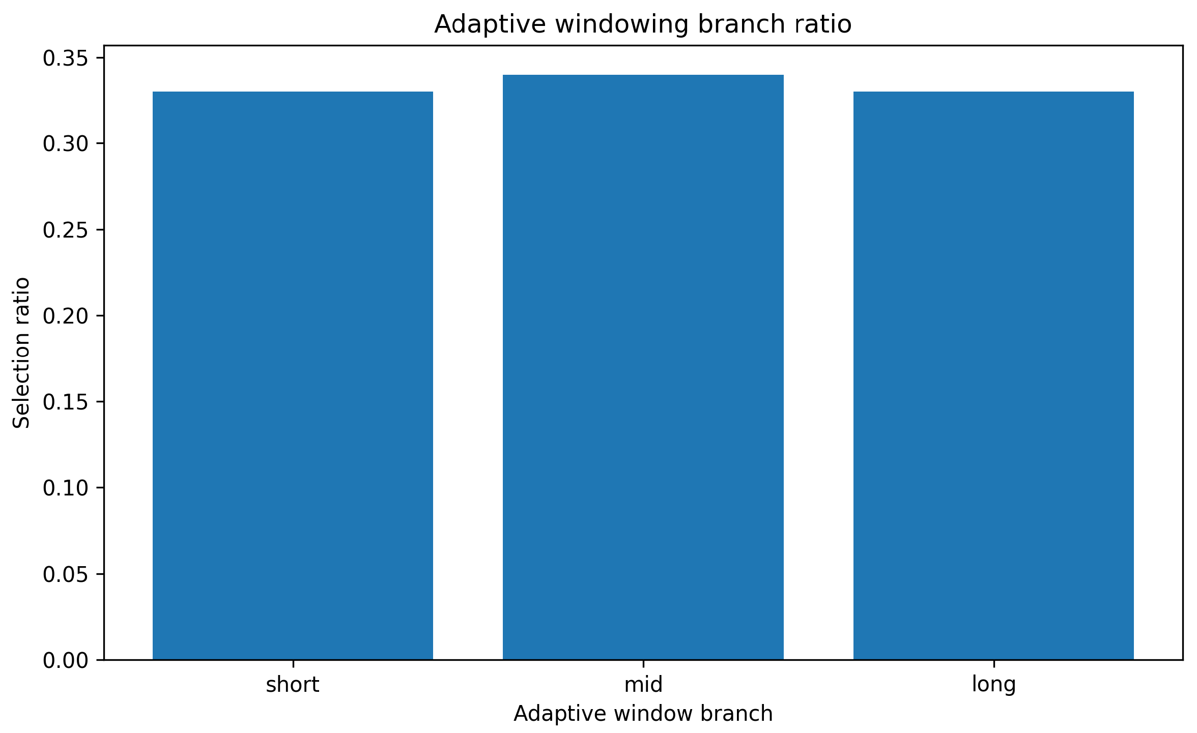
To further verify that the adaptive-window mechanism remained active under the present benchmark, we examined the saved branch decisions over the 22 test cells at both stage-resolved and aggregate levels. Figure 2 summarizes the branch ratios within five normalized aging-progress bins. The long-span branch is dominant in the first two bins (0–20% and 20–40%), the mid-span branch becomes most frequent in the middle bin (40–60%), and the short-span branch becomes dominant in the later bins (60–80% and 80–100%). This stage-resolved shift is consistent with the intended descriptive behavior of the adaptive-window rule under the present benchmark, namely that denser recent-history sampling becomes more frequent at later aging stages. For completeness, the aggregate branch counts across all saved decisions are shown in Figure 3: the short-span, mid-span, and long-span branches were selected 47,262, 48,676, and 47,258 times, respectively, corresponding to ratios of 33.01%, 33.99%, and 33.00%. Taken together, Figure 2 and Figure 3 indicate that the adaptive-window rule neither collapsed to a single branch nor remained stage-invariant under the present benchmark. These figures therefore support only that the adaptive-window rule remained active in use and changed descriptively with aging progress under the present benchmark; they should not be interpreted as causal validation of an aging-stage mechanism, of knee-region detection, or of a unique electrochemical explanation for why the rule helps.

Figure 2. Stage-resolved distribution of adaptive-window branch selections over normalized aging progress. Each target-cell trajectory is divided into five normalized aging-progress bins, and the short-, mid-, and long-span branch ratios are summarized within each bin. The figure is intended as descriptive evidence that branch usage changes over aging progress under the present benchmark; it should not be interpreted as direct electrochemical validation of knee-region behavior.

Figure 3. Aggregate selection ratios of the three adaptive-window branches on the 22 test cells. The short-, mid-, and long-span branches account for 33.01%, 33.99%, and 33.00% of the saved decisions, respectively.

4.5. Efficiency and Accuracy–Cost Trade-Off

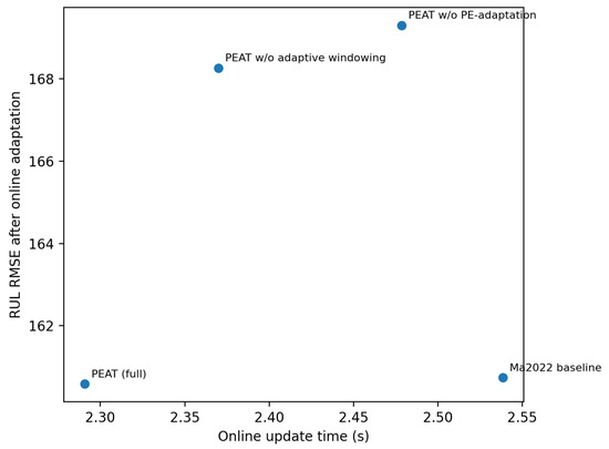
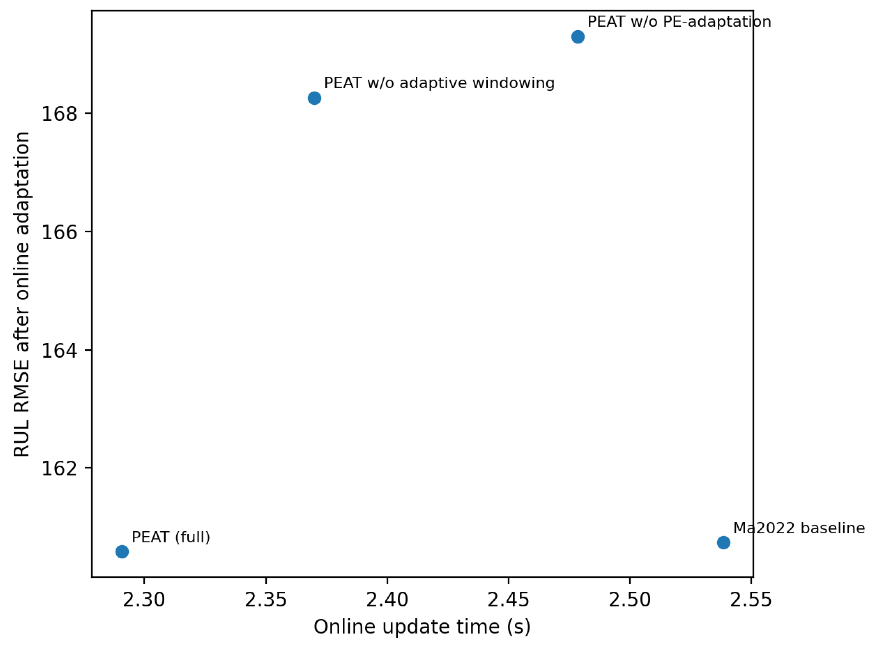
Online personalization should be evaluated not only by average prediction accuracy, but also by the update cost required to achieve that gain. Relative to the representative baseline [8], PEAT reduces the number of trainable parameters involved in online updating from 74,880 to 2193 and decreases the average update time per step from 2.54 s to 2.29 s. For battery-management deployment, this reduction matters because repeated updating must remain computationally manageable if personalization is to be used during operation. Figure 4 places the tested methods on a simple accuracy–cost plane, with online update time on the x-axis and post-adaptation RUL RMSE on the y-axis. Points closer to the lower-left corner correspond to a lower average error achieved with less update time. Under this comparison, the full PEAT setting lies closer to that corner than the representative baseline. The purpose of the figure is therefore not to claim an absolute advantage, but to show that the average benefit of personalization is still preserved when the update path is made lighter. For deployment, however, this average trade-off is only a first step; the next question is whether the gain is distributed safely across cells or is accompanied by harmful adaptation in a vulnerable subset.

Figure 4. Accuracy–cost trade-off. The x-axis represents the online update time, and the y-axis represents the RUL RMSE after online adaptation. The baseline point is taken from Ma et al. [8].

4.6. Per-Cell Error Change Under PEAT

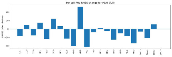
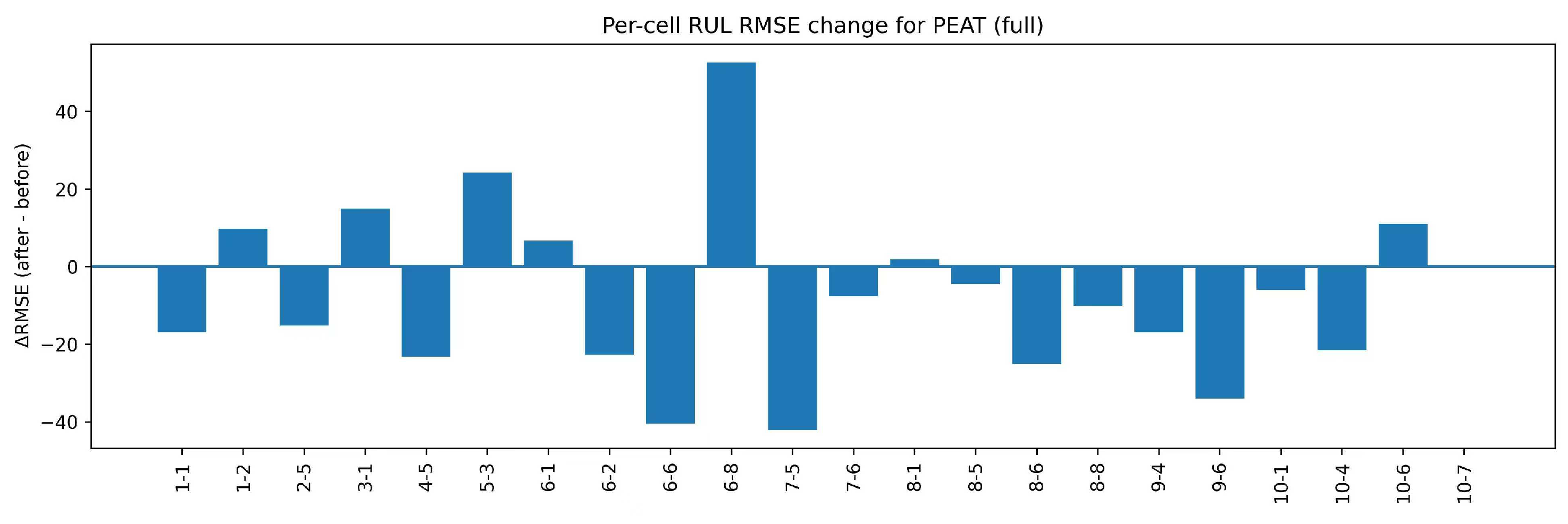
Average results can mask substantial cell-to-cell variation, which is critical for battery-management decisions based on online prognostics. To make this variation explicit, we examine the change in RMSE for each cell under PEAT. For a given cell, we define $\Delta$RMSE as RMSE(After) minus RMSE(Before). A negative $\Delta$RMSE indicates that online adaptation reduces the error, whereas a positive value indicates that it increases the error.

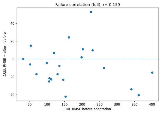
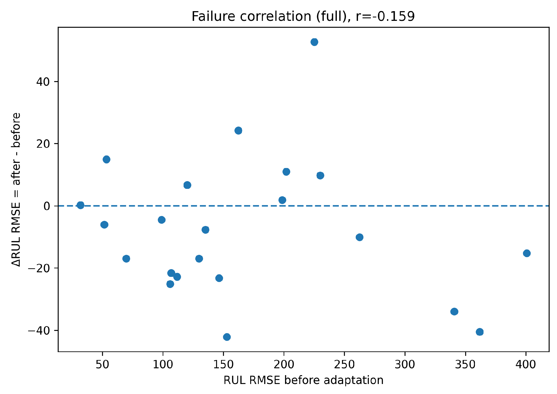
Figure 5 shows the $\Delta$RMSE values for the 22 cells. The full method reduces RMSE in 14 cells and increases it in 8 cells. At the cell level, the gain is therefore conditional rather than uniform. Larger pre-adaptation error can coincide with larger gains for some cells, but the present results do not support using pre-adaptation error alone as a reliable decision rule for when online updating should be applied. Online personalization should therefore not be treated as a uniform update step for all cells in battery prognostics. To further examine whether pre-adaptation error alone predicts adaptation benefit, we performed a simple per-cell correlation analysis between the RUL RMSE before adaptation and $\Delta$RMSE. The Pearson correlation was weak ($r=-0.159$). When the 22 test cells were grouped into low-, mid-, and high-before-RMSE subsets, the improvement rates were 71.4%, 62.5%, and 57.1%, respectively. Figure 6 further visualizes this weak association. These results indicate that larger pre-adaptation mismatch alone is not a sufficient predictor of whether online updating will be beneficial, which further motivates conservative update control.

Figure 5. Per-cell change in RUL RMSE under the full method. $\Delta \mathrm{RMSE}={\mathrm{RMSE}}_{\mathrm{After}}-{\mathrm{RMSE}}_{\mathrm{Before}}$; negative values indicate improvement.

Figure 6. Relationship between pre-adaptation RUL RMSE and $\Delta \mathrm{RMSE}$ under the full PEAT method. Here, $\Delta \mathrm{RMSE}={\mathrm{RMSE}}_{\mathrm{After}}-{\mathrm{RMSE}}_{\mathrm{Before}}$, and negative values indicate improvement after online adaptation. The weak Pearson correlation ($r=-0.159$) suggests that larger pre-adaptation error alone is not a sufficient predictor of adaptation benefit.

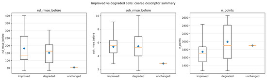
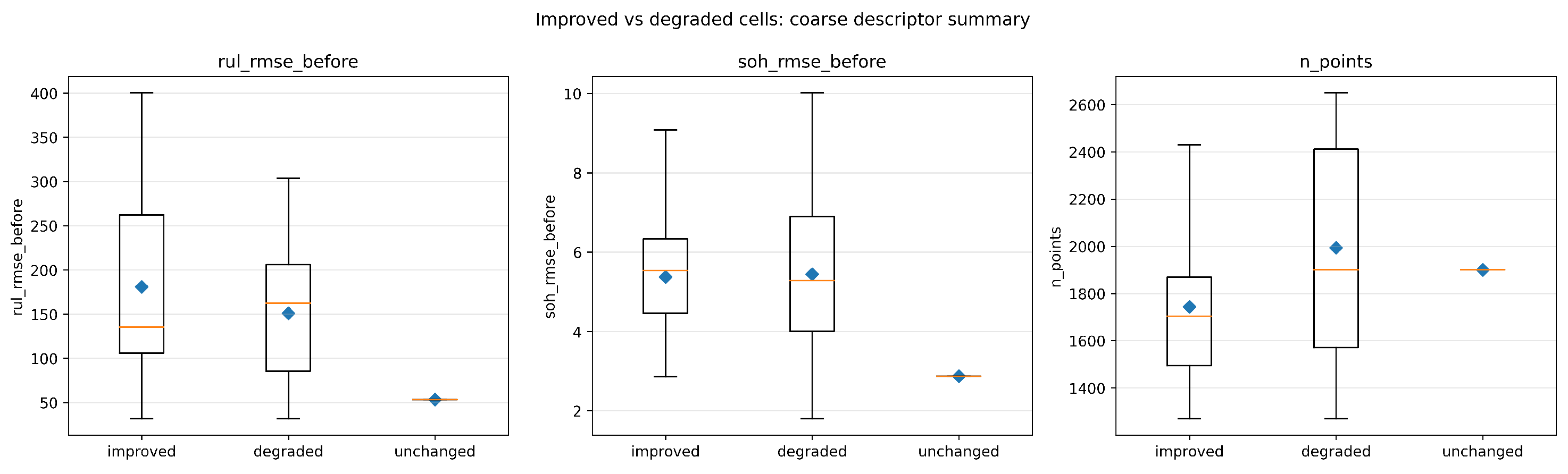
The present correlation analysis should therefore be interpreted as a minimal diagnostic under the available evidence rather than as a learned predictor of damaged cells. To complement this point, Figure 7 summarizes several descriptor-like quantities directly available from the saved full-method results, including pre-adaptation RUL RMSE, pre-adaptation SOH RMSE, and trajectory length (n_points), across improved, degraded, and unchanged outcomes. At the grouping level, improved outcomes are associated with larger and more dispersed pre-adaptation RUL mismatch, whereas the pre-adaptation SOH error distributions overlap substantially, and trajectory length does not clearly separate the groups. The added figure therefore provides coarse descriptor-level evidence for characterizing harmful-update cases under the available data, but it is not intended as a full feature-based taxonomy or a causal diagnosis of why individual cells deteriorate after updating.

Figure 7. Coarse descriptor summary comparing improved, degraded, and unchanged outcomes under the full PEAT method. Only descriptor-like quantities directly available from the saved result files are shown, including pre-adaptation RUL RMSE, pre-adaptation SOH RMSE, and trajectory length (n_points). Diamond markers denote the means, and the horizontal lines inside the boxes denote the medians. The figure is intended as grouping-level support for harmful-update characterization under the available evidence; it should not be interpreted as a full feature-based taxonomy or a causal diagnosis of failure modes.

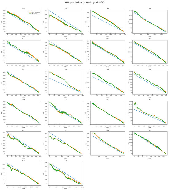
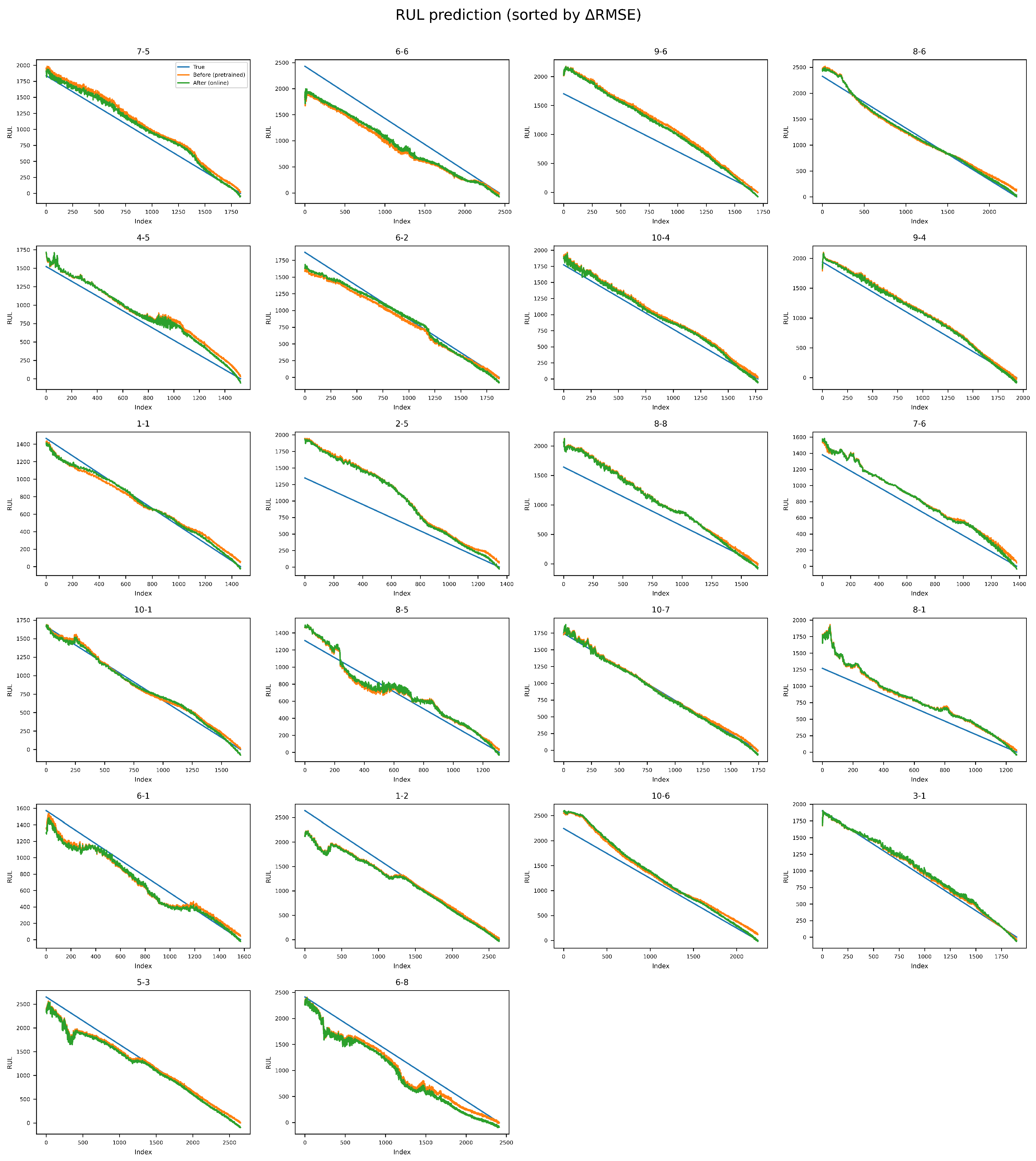
The full RUL trajectories of the 22 test cells are further visualized in Figure 8. The figure shows the ground-truth and predicted RUL curves before and after online adaptation, with the cells ordered by $\Delta$RMSE. This visualization links the average result to trajectory-level changes and provides context for the robustness analysis in Section 4.7 and the case studies in Section 4.8. An additional error-distribution analysis was performed for the full method. The mean RUL residual decreases from 25.99 cycles before adaptation to 9.98 cycles after adaptation, whereas the residual standard deviation changes only slightly, decreasing from 195.21 cycles to 191.20 cycles. This comparison indicates that online personalization should be evaluated not only by aggregate means, but also by distributional and worst-case behavior.

Figure 8. Qualitative RUL predictions for all 22 test cells (sorted by $\Delta$RMSE under PEAT). Each panel shows the ground-truth RUL curve and the predictions before (pre-trained) and after (online-adapted) personalization. The cells are ordered from the largest improvement (most negative $\Delta$RMSE) to the largest degradation (most positive $\Delta$RMSE).

Under the present causal online protocol, reliability is therefore assessed not only through average error, but also through per-cell variability, residual dispersion, degraded-cell counts, and worst-case degradation under selective updating. These diagnostics are emphasized because repeated random resampling across cells would not reflect the fixed target-cell online protocol considered here.

4.7. Robustness Analysis of Conservative Online Updating

An additional robustness study is conducted with a conservative online update policy, without changing the main PEAT design. This policy combines an update trigger, hold-out early stopping, and rollback. Section 4.6 shows that average improvement does not ensure safe personalization at the cell level. Relative to the no-adaptation reference used in the per-cell analysis, the original PEAT reduces the RUL RMSE on 14 of the 22 test cells but still increases it on the remaining 8. Its average RUL RMSE decreases from 168.10 to 160.58, whereas the worst-case degradation reaches 52.69.

To reduce harmful updates, we further evaluated a conservative online-update policy built on the same PEAT backbone. In the reported implementation, the target stream was processed in consecutive chunks of size 20, except when a chunk size of 21 was used to avoid a one-sample tail. Chunks that could not be split into at least six adaptation samples and three hold-out validation samples were skipped. The update-trigger threshold was calibrated on source-side validation chunks as the 75th percentile of the pre-update weighted capacity/SOH mismatch, which yielded $\tau \approx 1.95\times {10}^{-5}$ in the reported run. Once triggered, each chunk was split chronologically with a 70%/30% adaptation/hold-out ratio. The adapter path was then updated for at most 60 epochs using Adam (${10}^{-4}$) with patience 10. The adapted model was retained only when the post-update hold-out mismatch decreased by more than 1% relative to the pre-update score; otherwise, the parameters were rolled back to the pre-update state. In the saved Robust PEAT run, skipped chunks incurred no additional update cost, whereas retained and rolled-back updates required about 0.31 s and 0.30 s per chunk on average, respectively.

Table 3 summarizes the comparison between the original PEAT and Robust PEAT. Robust PEAT achieves an average RUL RMSE of 162.91, which is slightly higher than the 160.58 obtained by the original PEAT, indicating that part of the average gain is sacrificed. The number of degraded cells relative to the no-adaptation reference decreases from 8 to 6, one cell remains unchanged, and the worst-case degradation is reduced from 52.69 to 35.22. Compared with the original PEAT, Robust PEAT gives up part of the average gain in exchange for fewer harmful updates and lower worst-case degradation.

Table 3. Robustness comparison between the original PEAT and the conservative online updating variant (Robust PEAT). Panel (a) reports cell-level RUL stability relative to the no-adaptation reference. Negative mean $\Delta$RMSE values indicate lower average RUL error than the reference, whereas positive worst $\Delta$RMSE values indicate the most severe degradation case. Panel (b) summarizes the auxiliary SOH performance and the chunk-level update behavior of Robust PEAT.

(a) RUL and Stability Summary
Method	RMSE ↓	R2 ↑	Improved Cells	Degraded Cells	Mean ΔRMSE vs. No-Adaptation Reference	Worst ΔRMSE vs. No-Adaptation Reference
No-adaptation reference (Before)	168.10	0.8451	–	–	0.00	0.00
PEAT	160.58	0.8588	14/22	8/22	−7.51	52.69
Robust PEAT	162.91	0.8535	15/22	6/22	−5.19	35.22
(b) SOH Summary
Method			SOH RMSE ↓		R2 ↑	Improved SOH Cells
No-adaptation reference (Before)			5.74		0.9953	–
PEAT			4.18		0.9972	16/22
Robust PEAT			3.58		0.9980	20/22

In Panel (a), Robust PEAT has one unchanged cell relative to the no-adaptation reference. Chunk-level update behavior of Robust PEAT: 2036 total chunks; 1006 chunks skipped by the trigger; 987 chunks updated and retained; 34 chunks rolled back after adaptation; and 9 short chunks not updated. ↓ : lower is better; ↑ : higher is better.

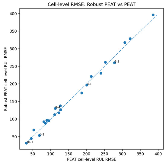
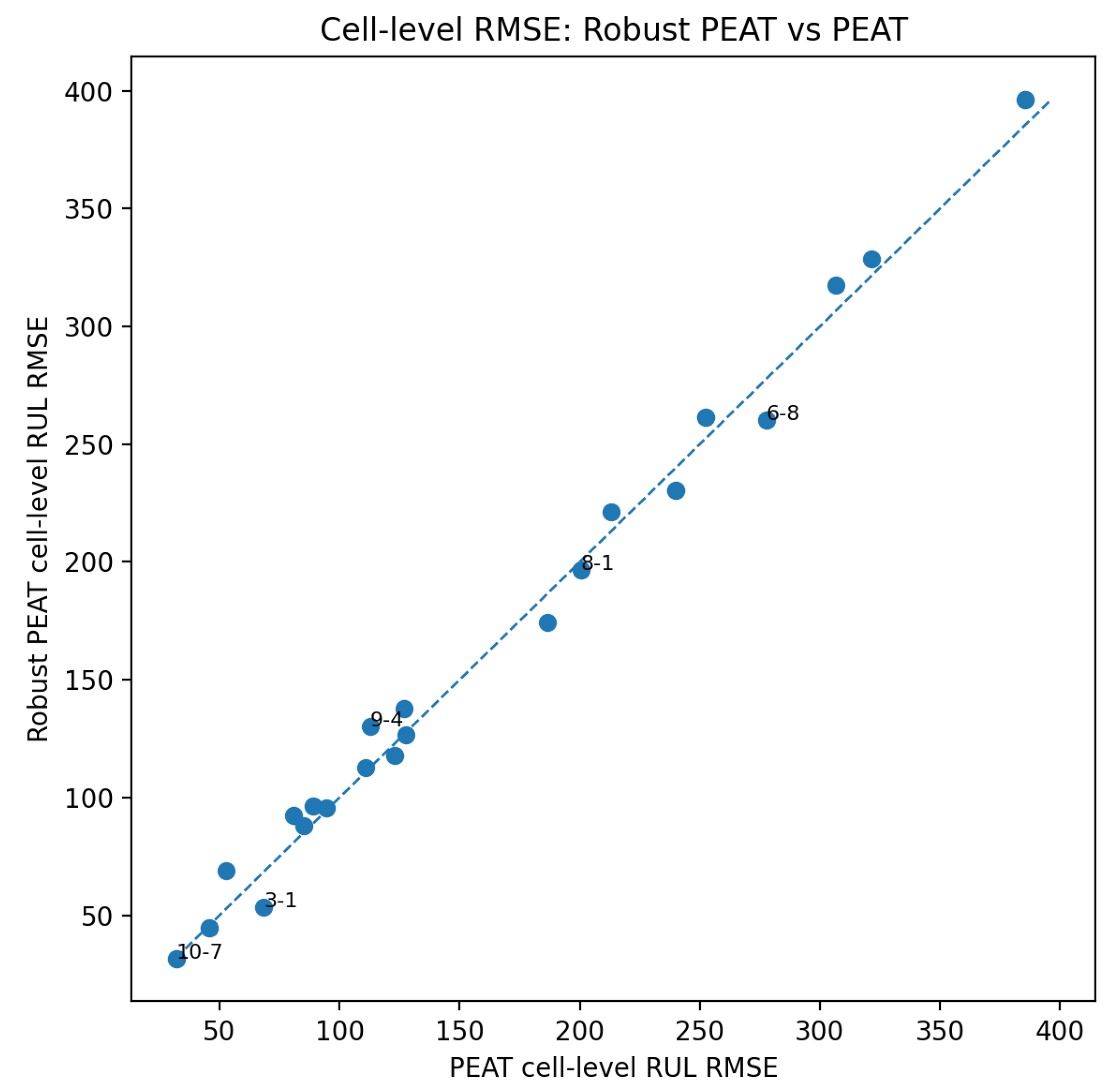
Figure 9 presents a cell-level comparison between the original PEAT and Robust PEAT. Cells below the diagonal have lower RUL RMSE under the conservative policy, whereas cells above the diagonal lose part of the larger gains achieved by the original PEAT. The distribution shows that Robust PEAT does not improve all cells uniformly. Instead, its benefit is concentrated on cells that are more vulnerable to harmful adaptation.

Figure 9. Cell-level RUL RMSE comparison between the original PEAT and Robust PEAT. The diagonal marks equal performance; points below it have lower RUL RMSE under Robust PEAT.

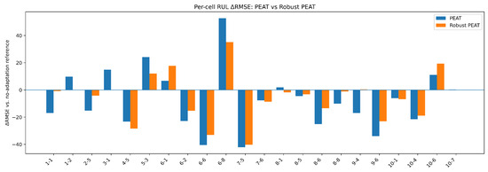
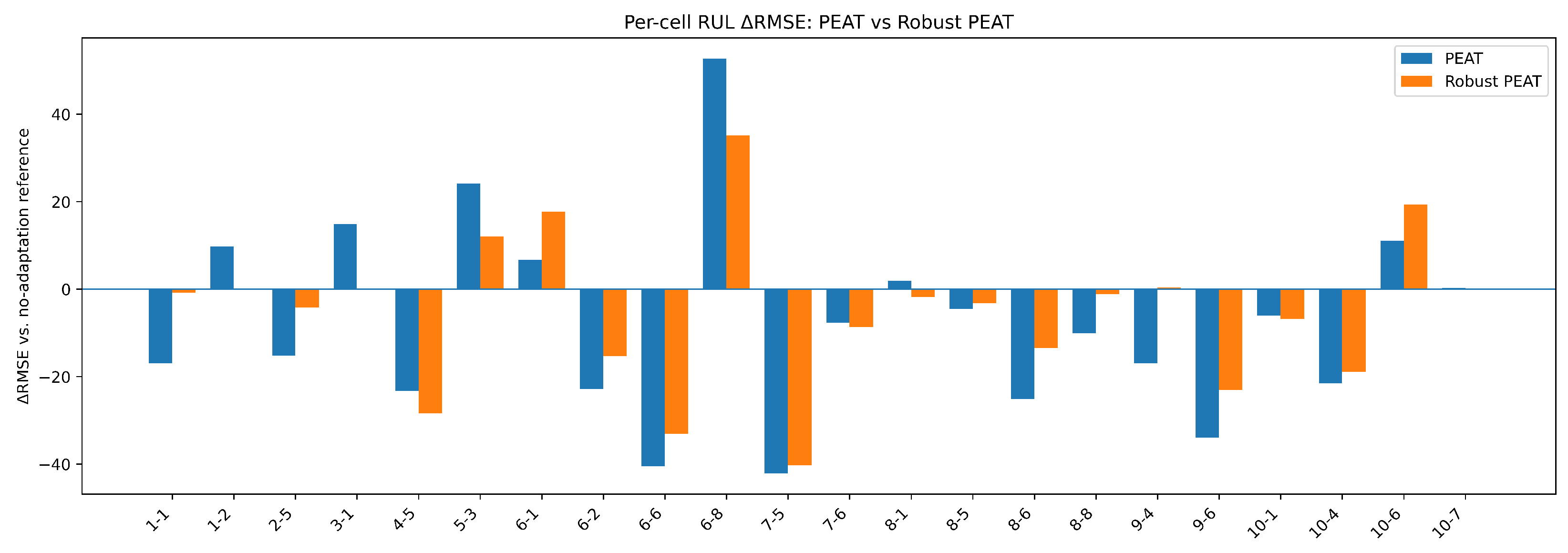
Figure 10 shows the per-cell change in RUL RMSE relative to the no-adaptation reference. Relative to the original PEAT, the conservative variant shortens the positive tail of the $\Delta$RMSE distribution and shifts some degraded cells to neutral or improved outcomes. This pattern matches the reduction in degraded cells from 8 to 6 and the decrease in worst-case degradation from 52.69 to 35.22.

Figure 10. Per-cell change in RUL RMSE relative to the no-adaptation reference for the original PEAT and Robust PEAT. Negative values denote improvement after online adaptation, and positive values denote degradation relative to the reference.

The average SOH RMSE decreases from 5.74 to 4.18 for the original PEAT and further to 3.58 for Robust PEAT, while the number of cells with improved SOH RMSE increases from 16 to 20. These aggregate changes are consistent with the view that the capacity-based trigger and rollback policy can also make the auxiliary SOH output more stable, although this effect is evaluated here only at the aggregate level.

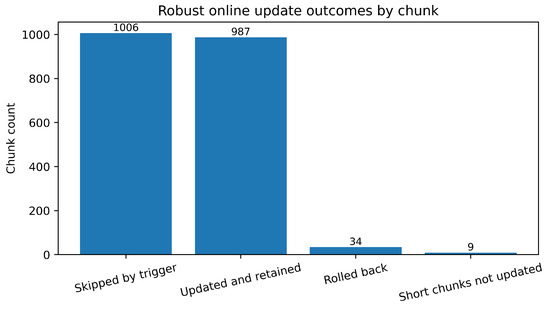
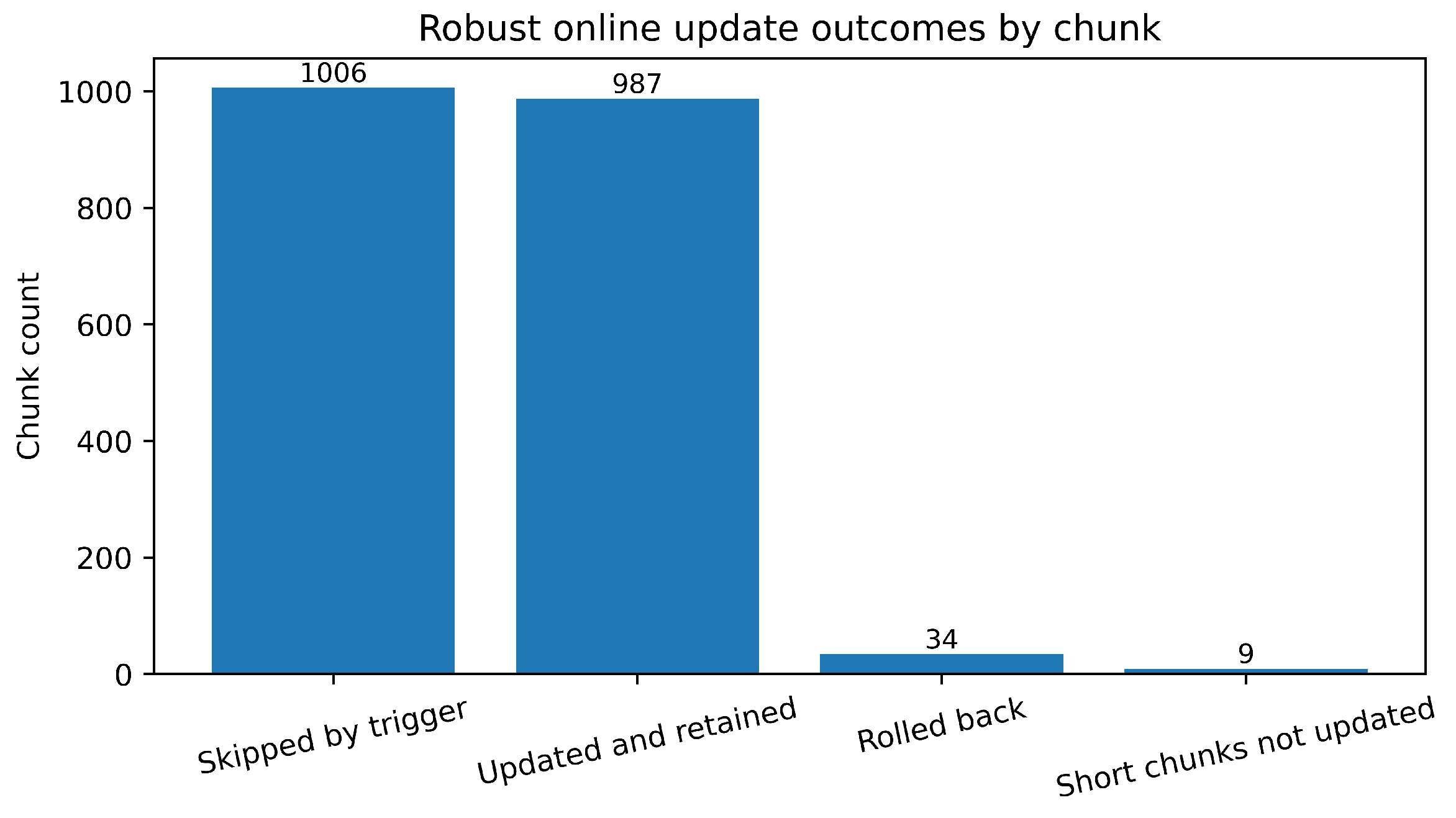
Figure 11 reports the chunk-level statistics associated with this behavior. Among the 2036 total chunks, 1006 are skipped by the trigger, 987 are updated and retained, 34 are rolled back after adaptation, and 9 short chunks are not updated. The counts show that online updating is not activated for nearly half of the chunks, and that only a small fraction of attempted updates are later rejected. These results suggest that online personalization does not need to be performed at every opportunity. Instead, a selective policy can retain much of the average benefit while reducing exposure to harmful updates.

Figure 11. Chunk-level decision distribution under Robust PEAT, including chunks skipped by the trigger, updated and retained, rolled back after adaptation, and short chunks not updated.

The robustness analysis is included because deployment-oriented evaluation in battery prognostics must consider more than average performance alone. Under the same backbone setting, lightweight online personalization improves the average result, while the conservative policy supports more selective updating with lower worst-case degradation and reduced harmful-update risk.

4.8. Case Studies

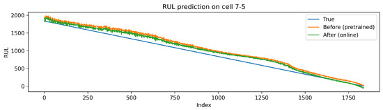
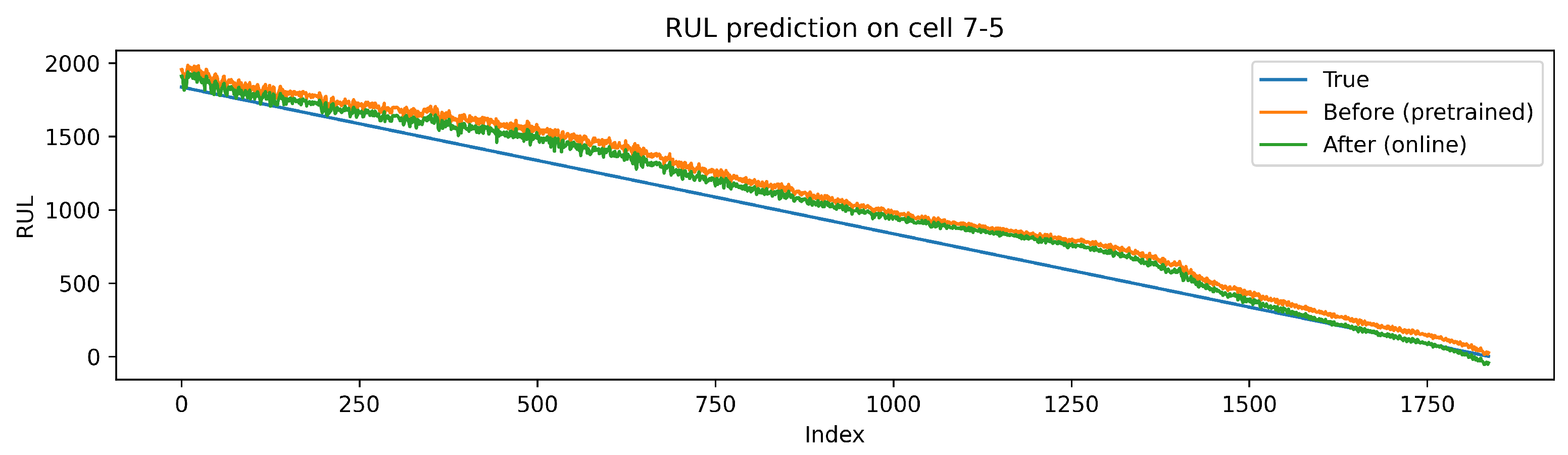
Figure 8 includes cells that illustrate both post-adaptation improvement and deployment risk. Figure 12 shows a cell with clear improvement. For cell 7-5, the RMSE decreases from 152.93 (Before) to 110.79 (After). After adaptation, the predicted curve follows the ground-truth trend more closely. This case matches the pattern noted in Section 4.6, where online personalization is more helpful when the pre-adaptation mismatch remains large.

Figure 12. Case study (improvement). RUL prediction for cell 7-5 before and after online adaptation under the full method.

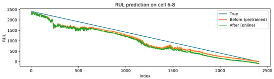
Figure 13 shows a cell whose prediction error increases after online adaptation. For cell 6-8, the RMSE rises from 225.07 (Before) to 277.75 (After), and the trajectory shows stronger localized fluctuations after updating. This case is consistent with the broader heterogeneity summarized in Section 4.6: harmful updates can still occur in a subset of cells, which motivates the conservative policy in Section 4.7. Together with Figure 5 and Figure 7, and Table 4, these examples provide only a coarse characterization of degraded cases rather than a feature-complete taxonomy or a causal diagnosis for each individual cell.

Figure 13. Case study (degradation). RUL prediction for cell 6-8 before and after online adaptation under the full method.

Table 4. Cells whose RUL RMSE increased after online adaptation under the full PEAT method. Here, $\Delta \mathrm{RMSE}={\mathrm{RMSE}}_{\mathrm{After}}-{\mathrm{RMSE}}_{\mathrm{Before}}$, and positive values indicate degradation after updating.

Cell	Before RUL RMSE	After RUL RMSE	ΔRMSE
6-8	225.07	277.75	52.69
5-3	162.33	186.53	24.20
3-1	53.46	68.40	14.94
10-6	202.03	213.06	11.04
1-2	230.09	239.86	9.77
6-1	120.05	126.74	6.69
8-1	198.52	200.38	1.87
10-7	31.83	32.08	0.26

The degraded cells under the full PEAT method are listed in Table 4. The table should be read together with Figure 5 and the representative degradation example in Figure 13.

4.9. SOH Results and Trade-Off

Table 5 highlights a limitation of the present design. Although the full method improves its own average SOH RMSE after online adaptation from 5.74 to 4.18, this value remains above the 2.57 reported for the representative baseline study. This gap is consistent with the current update design: during online adaptation, the direct RUL loss is disabled ($\lambda =0$), the RUL head remains frozen, and only the shared adapter together with the auxiliary SOH head is updated. Under this setting, the reported RUL gain is obtained indirectly through representation adjustment driven by the capacity/SOH path. The present evidence therefore supports a limited conclusion: the lightweight update path is useful for RUL-oriented personalization under the chosen benchmark, but it does not provide the best standalone SOH estimation. More task-aware weighting or partially decoupled update paths may reduce this gap, but these options are beyond the scope of the present work.

Table 5. SOH results (mean over 22 test protocols/cells). Baseline After values are from [8]; the corresponding Before results are not reported there.

Method	Before			After
	RMSE ↓	R2 ↑	MAPE (%) ↓	RMSE ↓	R2 ↑	MAPE (%) ↓
Ma et al. (2022) baseline [8]	–	–	–	2.57	0.999	0.176
PEAT (Full)	5.74	0.9953	0.420	4.18	0.9972	0.294

↓ : lower is better; ↑ : higher is better.

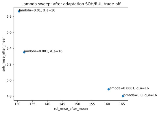
Additional sensitivity runs were performed with separate revision rerun utilities and saved as exploratory result bundles, whereas Table 1 and Table 2 report the main saved deployment comparison. The sweep values below therefore quantify within-sweep sensitivity under that separate rerun path; they are reported as exploratory support results rather than as replacement main results. In particular, the $\lambda =0$ sweep entry should be read as the shared-adapter result from the exploratory sweep bundle, not as a reprint of the main saved full-PEAT result in Table 1 and Table 2. When $\lambda$ was varied over $\{0,{10}^{-4},{10}^{-3},{10}^{-2}\}$, the after-adaptation RUL RMSE changed from 165.30 to 160.53, 132.27, and 130.55, whereas the corresponding SOH RMSE changed from 4.80 to 4.89, 5.35, and 5.86, respectively. The corresponding after-adaptation SOH/RUL trade-off is visualized in Figure 14. Within this exploratory sweep setting, the results indicate that the current update path does not support a uniformly beneficial multi-task setting, and that stronger RUL weighting can alter the SOH/RUL trade-off substantially.

Figure 14. After-adaptation SOH/RUL trade-off under different loss weights $\lambda$ with $d_a=16$. Increasing $\lambda$ improves RUL performance in this sweep, but worsens SOH RMSE, indicating a nontrivial multi-task trade-off in the current update path.

We additionally evaluated adapter bottleneck dimensions $d_a\in \{8,16,32\}$ under the same sweep setting. The after-adaptation RUL RMSE values were 165.94, 165.30, and 164.96, respectively, while the corresponding SOH RMSE values were 4.82, 4.80, and 4.69, with trainable parameters increasing from 1161 to 2193 and 4257. These results suggest that the observed behavior is not tied to a single bottleneck choice, although the sensitivity remains modest within this range.

Taken together, the sweep results above are consistent with a shared-update bottleneck in the present design, but they do not by themselves isolate whether the shared lightweight path contributes structurally to the observed SOH/RUL trade-off. To examine this point further, we added a decoupled-adapter control under the same benchmark, the same loss weight ($\lambda ={10}^{-4}$), and the same adapter bottleneck ($d_a=16$). This control was run in the same exploratory rerun setting as the $\lambda$-sweep and is therefore reported here as matched exploratory evidence rather than as a replacement for the main results in Table 1 and Table 2. In this control, the CNN–LSTM backbone remained unchanged, but the original shared lightweight update path was replaced with two task-specific lightweight branches for the RUL and SOH paths. Under this matched setting, the shared-adapter variant achieved an after-adaptation RUL RMSE of 160.53 and an after-adaptation SOH RMSE of 4.89, whereas the decoupled-adapter control achieved 98.67 and 4.71, respectively. At the same time, the decoupled control increased the number of trainable parameters from 2193 to 4397 and the mean online update time from 123.89 s to 493.09 s. The update-time values in Table 6 are therefore reported only as relative costs within this exploratory control, not as replacements for the per-step deployment cost reported in Section 4.5. These results indicate that the shared lightweight path is one contributing factor to the observed SOH/RUL trade-off under the present benchmark, while task-specific lightweight branches can partly alleviate this tension. This comparison, however, is used here only as structural support evidence and does not replace the main PEAT conclusion.

Table 6. Structural comparison between the shared-adapter and decoupled-adapter variants under the same exploratory Task-A rerun setting with $\lambda ={10}^{-4}$ and $d_a=16$. The decoupled variant uses separate lightweight branches for the RUL and SOH paths while keeping the same CNN–LSTM backbone. The update-time values reported here are mean per-cell rerun fine-tuning times within this exploratory control, not the per-step deployment update times reported in Section 4.5.

Method	After RUL RMSE ↓	After SOH RMSE ↓	Mean Update Time (s) ↓	Trainable Params ↓
Shared adapter	160.53	4.89	123.89	2193
Decoupled adapter	98.67	4.71	493.09	4397

↓ : lower is better.

4.10. Discussion

Under the fixed-backbone and fixed-input setting, PEAT does not aim to replace existing RUL predictors with a universally superior model. Its role is to provide a lighter online update path when a pre-trained global model remains mismatched to a target cell. In battery management, average improvement is meaningful only when it is obtained with a manageable update cost and an acceptable adaptation risk. The cell-level results further show that the gain is conditional rather than universal: some cells with larger pre-adaptation mismatch can benefit more from personalization, whereas cells that are already well tracked or locally noisy may deteriorate after updating.

The present evidence is also limited to the representative HUST benchmark [8] used here, with a single dataset, a fixed train–test split, and a fixed fast-charging protocol and ambient temperature. No validation across dynamically varying operating conditions was performed in the present study. Accordingly, the thresholds in Equation (3) should be interpreted as benchmark-specific heuristics under this controlled setting, rather than as operating-condition-invariant constants or as evidence of validated generalization beyond the present benchmark.

The results reported above reflect trade-offs rather than uniform dominance. Adaptation benefit, update cost, and harmful-update risk need to be considered together. Section 4.5, Section 4.6 and Section 4.7 show that PEAT improves the first two on average under the same basic setting, whereas the conservative variant in Section 4.7 reduces the third through selective updating. The SOH results add a further boundary condition: the shared lightweight adaptation path does not support RUL and SOH equally well. A deployment-ready personalization scheme for battery prognostics therefore still requires lightweight adaptation together with update triggering, rollback control, and more careful multi-task balancing.

5. Conclusions

This work addresses a practical issue in deployment-oriented battery prognostics: how to make personalization less burdensome under a representative CNN–LSTM online-transfer setting without changing the backbone or fixed input length. The experiments suggest that this goal can be achieved to a useful but limited extent. PEAT reduces the number of trainable parameters involved in online updating, slightly shortens the per-step update time, and still improves the average RUL result after adaptation. At the same time, the evaluation shows that average improvement alone is not sufficient for battery-management deployment: some cells still deteriorate after updating, and the conservative variant indicates that part of the average gain can be traded for lower worst-case degradation and fewer harmful updates. These results indicate that under the same baseline setting, online personalization can move toward a better balance among accuracy benefit, update cost, and adaptation risk. The remaining SOH gap further indicates that more selective updating and better coordination between tasks are still needed.

References

- International Energy Agency. Batteries and Secure Energy Transitions; International Energy Agency: Paris, France, 2024. [Google Scholar]
- Che, Y.; Hu, X.; Lin, X.; Guo, J.; Teodorescu, R. Health prognostics for lithium-ion batteries: Mechanisms, methods, and prospects. Energy Environ. Sci. 2023, 16, 338–371. [Google Scholar] [CrossRef] [Scilit]
- Hu, X.; Xu, L.; Lin, X.; Pecht, M. Battery lifetime prognostics. Joule 2020, 4, 310–346. [Google Scholar] [CrossRef] [Scilit]
- Xie, Y.; Wang, S.; Zhang, G.; Takyi-Aninakwa, P.; Fernandez, C.; Blaabjerg, F. A review of data-driven whole-life state of health prediction for lithium-ion batteries: Data preprocessing, aging characteristics, algorithms, and future challenges. J. Energy Chem. 2024, 97, 630–649. [Google Scholar] [CrossRef] [Scilit]
- Ge, M.-F.; Liu, Y.; Jiang, X.; Liu, J. A review on state of health estimations and remaining useful life prognostics of lithium-ion batteries. Measurement 2021, 174, 109057. [Google Scholar] [CrossRef] [Scilit]
- Devie, A.; Baure, G.; Dubarry, M. Intrinsic variability in the degradation of a batch of commercial 18650 lithium-ion cells. Energies 2018, 11, 1031. [Google Scholar] [CrossRef] [Scilit]
- Diao, W.; Kim, J.; Azarian, M.H.; Pecht, M. Degradation modes and mechanisms analysis of lithium-ion batteries with knee points. Electrochim. Acta 2022, 431, 141143. [Google Scholar] [CrossRef] [Scilit]
- Ma, G.; Xu, S.; Jiang, B.; Cheng, C.; Yang, X.; Shen, Y.; Yang, T.; Huang, Y.; Ding, H.; Yuan, Y. Real-time personalized health status prediction of lithium-ion batteries using deep transfer learning. Energy Environ. Sci. 2022, 15, 4083–4094. [Google Scholar] [CrossRef] [Scilit]
- Liu, K.; Peng, Q.; Che, Y.; Zheng, Y.; Li, K.; Teodorescu, R.; Widanage, D.; Barai, A. Transfer learning for battery smarter state estimation and ageing prognostics: Recent progress, challenges, and prospects. Adv. Appl. Energy 2023, 9, 100117. [Google Scholar] [CrossRef] [Scilit]
- Che, Y.; Zheng, Y.; Onori, S.; Hu, X.; Teodorescu, R. Increasing generalization capability of battery health estimation using continual learning. Cell Rep. Phys. Sci. 2023, 4, 101743. [Google Scholar] [CrossRef] [Scilit]
- Kim, S.W.; Oh, K.-Y.; Lee, S. Novel informed deep learning-based prognostics framework for on-board health monitoring of lithium-ion batteries. Appl. Energy 2022, 315, 119011. [Google Scholar] [CrossRef] [Scilit]
- Qin, H.; Fan, X.; Fan, Y.; Wang, R.; Shang, Q.; Zhang, D. A computationally efficient approach for the state-of-health estimation of lithium-ion batteries. Energies 2023, 16, 5414. [Google Scholar] [CrossRef] [Scilit]
- Wu, W.; Chen, Z.; Liu, W.; Zhou, D.; Xia, T.; Pan, E. Battery health prognosis in data-deficient practical scenarios via reconstructed voltage-based machine learning. Cell Rep. Phys. Sci. 2025, 6, 102442. [Google Scholar] [CrossRef] [Scilit]
- Bifet, A.; Gavaldà, R. Learning from time-changing data with adaptive windowing. In Proceedings of the 2007 SIAM International Conference on Data Mining, Minneapolis, MN, USA, 26–28 April 2007; pp. 443–448. [Google Scholar]
- Yang, B.; Qian, Y.; Li, Q.; Chen, Q.; Wu, J.; Luo, E.; Xie, R.; Zheng, R.; Yan, Y.; Su, S.; et al. Critical summary and perspectives on state-of-health of lithium-ion battery. Renew. Sustain. Energy Rev. 2024, 190, 114077. [Google Scholar] [CrossRef] [Scilit]
- Kumar, R.; Das, K. Lithium battery prognostics and health management for electric vehicle application—A perspective review. Sustain. Energy Technol. Assess. 2024, 65, 103766. [Google Scholar] [CrossRef] [Scilit]
- dos Reis, G.; Strange, C.; Yadav, M.; Li, S. Lithium-ion battery data and where to find it. Energy AI 2021, 5, 100081. [Google Scholar] [CrossRef] [Scilit]
- Mayemba, Q.; Mingant, R.; Li, A.; Ducret, G.; Venet, P. Aging datasets of commercial lithium-ion batteries: A review. J. Energy Storage 2024, 83, 110560. [Google Scholar] [CrossRef] [Scilit]
- Li, X.; Yu, D.; Byg, V.S.; Ioan, S.D. The development of machine learning-based remaining useful life prediction for lithium-ion batteries. J. Energy Chem. 2023, 82, 103–128. [Google Scholar] [CrossRef] [Scilit]
- Zhao, J.; Feng, X.; Pang, Q.; Wang, J.; Lian, Y.; Ouyang, M.; Burke, A.F. Battery prognostics and health management from a machine learning perspective. J. Power Sources 2023, 581, 233474. [Google Scholar] [CrossRef] [Scilit]
- Zhang, Y.; Li, Y.-F. Prognostics and health management of lithium-ion battery using deep learning methods: A review. Renew. Sustain. Energy Rev. 2022, 161, 112282. [Google Scholar] [CrossRef] [Scilit]
- Lyu, D.; Zhang, B.; Zio, E.; Xiang, J. Battery cumulative lifetime prognostics to bridge laboratory and real-life scenarios. Cell Rep. Phys. Sci. 2024, 5, 102164. [Google Scholar] [CrossRef] [Scilit]
- Shu, X.; Shen, J.; Li, G.; Zhang, Y.; Chen, Z.; Liu, Y. A flexible state-of-health prediction scheme for lithium-ion battery packs with long short-term memory network and transfer learning. IEEE Trans. Transp. Electrif. 2021, 7, 2238–2248. [Google Scholar] [CrossRef] [Scilit]
- Sahoo, S.; Hariharan, K.S.; Agarwal, S.; Swernath, S.B.; Bharti, R.; Han, S.; Lee, S. Transfer learning based generalized framework for state of health estimation of Li-ion cells. Sci. Rep. 2022, 12, 13173. [Google Scholar] [CrossRef] [Scilit]
- Yang, Y.; Xu, Y.; Nie, Y.; Li, J.; Liu, S.; Zhao, L.; Yu, Q.; Zhang, C. Deep transfer learning enables battery state of charge and state of health estimation. Energy 2024, 294, 130779. [Google Scholar] [CrossRef] [Scilit]
- Gu, B.; Liu, Z. Transfer learning-based remaining useful life prediction method for lithium-ion batteries considering individual differences. Appl. Sci. 2024, 14, 698. [Google Scholar] [CrossRef] [Scilit]
- Lin, T.; Chen, S.; Harris, S.J.; Zhao, T.; Liu, Y.; Wan, J. Investigating explainable transfer learning for battery lifetime prediction under state transitions. eScience 2024, 4, 100280. [Google Scholar] [CrossRef] [Scilit]
- Ji, S.; Zhang, Z.; Stein, H.S.; Zhu, J. Flexible health prognosis of battery nonlinear aging using temporal transfer learning. Appl. Energy 2025, 377, 124766. [Google Scholar] [CrossRef] [Scilit]
- Wu, X.; Chen, J.; Tang, H.; Xu, K.; Shao, M.; Long, Y. Robust online estimation of state of health for lithium-ion batteries based on capacities under dynamical operation conditions. Batteries 2024, 10, 219. [Google Scholar] [CrossRef] [Scilit]
- Gama, J.; Žliobaitė, I.; Bifet, A.; Pechenizkiy, M.; Bouchachia, A. A survey on concept drift adaptation. ACM Comput. Surv. 2014, 46, 44. [Google Scholar] [CrossRef] [Scilit]
- Ni, Y.; Li, X.; Zhang, H.; Wang, T.; Song, K.; Zhu, C.; Xu, J. Online identification of knee point in conventional and accelerated aging lithium-ion batteries using linear regression and Bayesian inference methods. Appl. Energy 2025, 388, 125646. [Google Scholar] [CrossRef] [Scilit]
- Houlsby, N.; Giurgiu, A.; Jastrzebski, S.; Morrone, B.; de Laroussilhe, Q.; Gesmundo, A.; Attariyan, M.; Gelly, S. Parameter-efficient transfer learning for NLP. In Proceedings of the 36th International Conference on Machine Learning, Long Beach, CA, USA, 9–15 June 2019; pp. 2790–2799. [Google Scholar]
Disclaimer/Publisher’s Note: The statements, opinions and data contained in all publications are solely those of the individual author(s) and contributor(s) and not of MDPI and/or the editor(s). MDPI and/or the editor(s) disclaim responsibility for any injury to people or property resulting from any ideas, methods, instructions or products referred to in the content. |
© 2026 by the authors. Licensee MDPI, Basel, Switzerland. This article is an open access article distributed under the terms and conditions of the Creative Commons Attribution (CC BY) license.