Optimization of a Wind Turbine Gearbox Design Reducing Component Damage Risk Considering Different Electrical Faults

Abstract

Wind turbine (WT) drivetrains are exposed to high dynamic loads, especially caused by grid and converter faults. Those loads increase the frictional energy in the contact zone of the gearbox bearings and gear wheels and, thus, theoretically, the probability of failure of the gearbox before the WTs reach their service lifetime. To increase the robustness against grid and converter faults, gearboxes can be designed to include these as special load cases. The critical parts of gearboxes regarding the influence of grid and converter faults are the components of the fast-rotating gearbox side. This paper introduces an optimization procedure for the high-speed shaft (HSS) components of a WT gearbox, considering several electrical faults as special load cases. The basis for data collection in this work is a validated multi-body simulation (MBS) model of a WT drivetrain. Initially, a test plan is formulated using Latin hypercube sampling (LHS). Based on the simulation results generated with the detailed MBS model according to the defined test plan, computationally efficient surrogate models are derived that link the design parameters with the objectives of the optimization. The surrogate models are employed to optimize the microgeometry of the gearbox. The process is done for several electrical faults. With the optimization, the risk of damage to the gear wheels can be reduced by 28% with a reduced or equal risk of damage to the HSS bearing, depending on the load case. It is also shown via comparison that the optimal design for one critical fault simultaneously leads to a sufficient improvement for other electrical faults (max. 4% reduction in improvement of objectives). Thus, it is sufficient to do the optimization regarding electrical faults only for one critical fault, reducing the necessary computational effort significantly.

1. Introduction

Germany is aiming for greenhouse gas neutrality in the long term. For the energy sector, this means achieving decarbonization by 2050 [1]. To this end, the proportion of renewable energy in the electricity mix must increase, while its costs must decrease. One major pillar for renewable energy in Germany is wind energy, which is already among the most cost-competitive sources of electricity. To further support the expansion of wind energy, improving the economic efficiency of WTs remains important. One way of achieving this is to minimize the downtime of WTs. The longest downtimes in WTs occur due to gearbox faults [2]. Within gearboxes, the faults can most often be attributed to the components of the HSS and the intermediate shaft (IMS) of the gearbox, especially the bearings, but also the gear wheels. This paper, therefore, examines the gear wheels on the HSS and IMS as well as the floating bearing of the HSS (which is designed as a cylindrical rolling bearing) of a 2.75 MW research nacelle.

Taking electrical fault conditions into account can increase the future robustness of gearboxes. In addition to the nominal operation, which is well covered in the current design guidelines for WT gearboxes, special load cases due to electrical faults must be considered as well in the future, since they might introduce extraordinary torque ripples dependent on the grid connection of the WT [3]. The macroscopic gearbox design is determined by nominal and partial load operation. Preliminary work has already shown that safety against gear damage, such as micropitting, scuffing, tooth flank breakage and tooth root breakage, can be increased during electrical faults by varying the microgeometry of the spur gear teeth, and the risk of smearing can be reduced via a variation in the clearance in the cylindrical roller bearing [4].

In this work, four different load cases are analyzed to investigate the electrical faults in more detail. Three of the load cases result from grid faults acting on a doubly fed induction generator (DFIG) with a partial-size power converter. These do not occur in the system of the WT, but in the power grid, and, therefore, have an external cause. The grid faults affect the DFIG and lead to dynamic generator torque excitations, with amplitudes significantly higher than the nominal torque. As a fourth load case, a short circuit in a full converter, i.e., an internal WT fault, is considered.

A method has been developed to optimize the microgeometry considering the different electrical faults. The goal is an increased robustness of the HSS components against four different fault load cases. The aim is to identify a gear geometry that will make the gearbox more robust in all four load cases. For this purpose, a test plan is first developed, according to which MBSs are carried out by systematically varying the parameters. The simulation data is then used to create computationally efficient surrogate models, which establish a mathematical relationship between the parameters and the objectives. Multi-criteria optimization using the surrogate models selects parameters for an optimized gearbox design. The four fault load cases are considered when selecting the optimized gearbox design.

2. Materials and Methods

In previous studies, the selected components were optimized considering a single fault load case. To consider multiple electrical faults, a global optimization for different load cases is performed. Thus, a toolchain is used, which includes the simulation model, a design of experiments (DoE), a simulation series, surrogate models and the final optimization.

2.1. Multi-Body Simulation

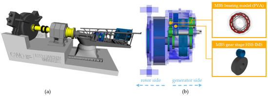
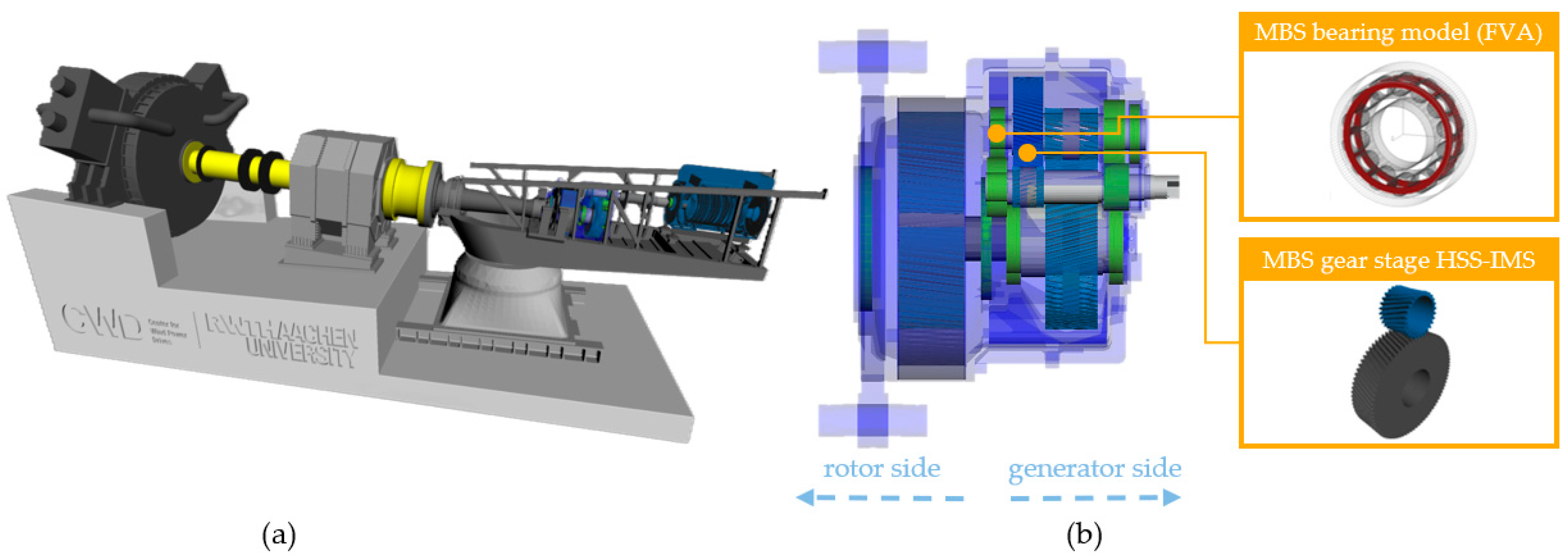
To calculate the damage criteria, a validated MBS model of a 2.75 MW research nacelle is used [5,6]. The test rig setup includes the entire drivetrain of the WT from the main shaft to the generator (Figure 1) [7]. A detailed sub-model of the HSS cylindrical rolling bearing is built into the model. The sub-model is created beforehand with a calculation module for rolling bearings, LaMBDA (bearing multi-body calculation and dynamic analysis) [8]. The MBS model has already been validated in previous work [5,6].

Figure 1. MBS model of the full research nacelle (a) and the gearbox with a detailed bearing and gear stage (b) [3].

2.2. Quantification of the Damage Risk

Damage mechanisms in the gear wheels on the HSS and IMS, as well as in the HSS floating cylindrical roller bearing, are considered. Common gear failures, which can be calculated according to ISO 6336 (see Table 1), include micropitting, scuffing, tooth flank fracture, and tooth breakage [9,10,11,12].

Table 1. Definition of the safety factors of the gear wheels.

Safety Factor	Definition
Safety against micropitting	$S_{\lambda }={\displaystyle \frac{{\lambda }_{GF,min}}{{\lambda }_{GFP}}}$	[9]
Safety against scuffing	$S_B={\displaystyle \frac{{\theta }_S-{\theta }_{Oil}}{{\theta }_{Bmax}-{\theta }_{Oil}}}$	[10]
Safety against tooth flank fracture	$S_{FF}={\displaystyle \frac{0.8}{A_{FF,max}}}$	[11]
Safety against tooth breakage	$S_F={\displaystyle \frac{{\sigma }_{FG}}{{\sigma }_F}}$	[12]

$S_{\lambda }$ is defined by the locally specific lubricant film thickness ${\lambda }_{GF,min}$ and the permissible specific lubricant film thickness. The definition of $S_B$ considers the experimentally determined scuffing temperature ${\mathsf{\Theta }}_S$, the oil temperature ${\mathsf{\Theta }}_{Oil}$ and the maximum contact temperature ${\mathsf{\Theta }}_{B,max}$. $S_{FF}$ is defined by the quotient of the threshold of 0.8 and the maximum local material exposure $A_{FF,max}$. Tooth root stress ${\sigma }_F$ and the permissible bending stress is used to calculate $S_F$.

For bearings, the power per loaded area is one of the criteria of many damage patterns like WEC, smearing or rehardening. The power P per loaded area A is quantified using Equation (1) [13].

$${\left({\displaystyle \frac{P}{A}}\right)}_{max}=\max (0.5\cdot \mu \left(t\right)\cdot p_{max}\left(t\right)\cdot (\Delta u(t)))$$

(1)

In this equation, $\mu$ is the coefficient of friction, $p_{max}$ is the maximum Hertzian pressure and $\Delta u$ is the relative velocity between the two contact surfaces.

2.3. Design of Experiments

Since the generation of the data has a high impact on the computational effort, an efficient DoE is of great interest. Therefore, Latin hypercube sampling (LHS) is used in this work. LHS is suitable for a high number of factors. First, a Latin hypercube design (LHD) is created. With the number of test runs $n_r$ and the number of factors $n_f$, which results in an $n_r\times n_f$ matrix, where each row and column is a random permutation of the natural numbers {1, 2, 3, …, $n_r$}. Subtracting a random number from the range [0, 1) from each entry of the LHD and dividing the result by the number of trials yields a Latin hypercube sample. The LHS in this work is implemented by using the MATLAB R2022b function lhsdesign. Quadratic regression models with twelve factors are created below. This results in 91 degrees of freedom. Therefore, at least 91 simulations with different parameter configurations are required. After balancing accuracy against computational effort, a design of experiments comprising 136 runs is defined. When creating the LHS, the aim is a low correlation between the factor combinations. To ensure this, the Pearson correlation r is calculated (Equation (2)).

$$r={\displaystyle \frac{K_{xy}}{{\sigma }_x^2\cdot {\sigma }_y^2}},r\in [-1,1]$$

(2)

It describes the dependence of the two variables x and y on each other. $K_{xy}$ is the empirical covariance (Equation (3)).

$$K_{xy}={\displaystyle \frac{1}{n_r}}\cdot \sum _{i=1}^{n_r}\left(x_i-\overline{x}\right)\cdot \left(y_i-\overline{y}\right)$$

(3)

The values $\overline{x}$ and $\overline{y}$ represent the mean values of the two variables for which the correlation is determined. New samples are created iteratively until a correlation of less than 0.001 is achieved [14].

The limits of the individual parameters are based on preliminary investigations and are listed in Table 2. The reference parameters are those of the research nacelle on which the MBS model is based.

Table 2. Variable boundaries of the parameter space.

Component	Influencing Parameter	Lower Boundary (LB)	Upper Boundary (UB)	Reference	Unit
Gear wheel (HSS)	Profile shift coefficient $x_{HSS}$	−0.19	0.81	0.11	-
Gear wheel (HSS)	Tip relief $C_{a,HSS}$	40	200	40	$\mathsf{\mu }\mathrm{m}$
Gear wheel (HSS)	Profile crowning $C_{\alpha ,HSS}$	10	110	20	$\mathsf{\mu }\mathrm{m}$
Gear wheel (HSS)	Flank line crowning $C_{b,HSS}$	0	50	50	$\mathsf{\mu }\mathrm{m}$
Gear wheel (HSS)	Flank line slope modification $f_{H\beta ,HSS}$	0.02948	0.57	0.11055	$\mathrm{m}\mathrm{r}\mathrm{a}\mathrm{d}$
Gear wheel (IMS)	Tip relief $C_{a,IMS}$	0	120	30	$\mathsf{\mu }\mathrm{m}$
Gear wheel (IMS)	Profile crowning $C_{\alpha ,IMS}$	0	100	0	$\mathsf{\mu }\mathrm{m}$
Gear wheel (IMS)	End relief $l_{e,IMS}$	0	50	25	$\mathsf{\mu }\mathrm{m}$
Gear wheel (IMS)	End relief width $b_{e,IMS}$	0	70	35	$\mathrm{m}\mathrm{m}$
Gear wheel (IMS)	Flank line crowning $C_{b,IMS}$	0	50	0	$\mathsf{\mu }\mathrm{m}$
Gear wheel (IMS)	Flank line slope modification $f_{H\beta ,IMS}$	−0.16583	0.38693	0.11055	$\mathrm{m}\mathrm{r}\mathrm{a}\mathrm{d}$
Rolling bearing	Radial clearance $c_R$	0	117.5	117.5	$\mathsf{\mu }\mathrm{m}$

2.4. Regression

To create surrogate models that describe the correlation between the geometry parameters and the risk of damage, basic regression approaches are used. Mathematical correlations are created between the objectives y and the design parameters x for optimization purposes. The regression model for the objective $y_i$ is given by the factors $x_{ij}$, the correlations $x_i{x}_j$ and the model constants $c$. It is formulated according to Equation (4). Epsilon ($ϵ$) describes the deviation between the regression model and the actual behavior of the system, which cannot be described by x.

$$y_i=c_0+c_1{x}_{i1}+c_2{x}_{i1}^2+c_3{x}_{i2}+c_4{x}_{i2}^2+\cdots +c_k{x}_{i1}{x}_{i2}+\cdots +{ϵ}_i$$

(4)

These regression models are generated via sequential floating forward selection. Linear and quadratic dependencies of the objectives on the factors are considered. Terms are gradually added to or removed from the model until no significant model improvement is achieved.

This approach is supplemented by a robust regression. The deviations (residuals r) of the training data from the model prediction are determined based on a calculated regression model. As long as $\left|r\right|<3\sigma$ applies to the largest residual in terms of amount, where $\sigma$ is the standard deviation of the residuals, the corresponding data point is removed from the training data. A regression is then carried out again with the new training data set [14].

The R² quality criterion can be used to evaluate regression models. It is calculated using the objective of the training data ($y_i$), the associated model prediction ($\widehat{y_i}$), and the number of measurements ($n_r$), according to Equation (5).

$$R^2={\displaystyle \frac{S{S}_R}{S{S}_T}}=1-{\displaystyle \frac{S{S}_E}{S{S}_T}}=1-{\displaystyle \frac{{\sum }_{i=1}^{n_r}{\left(y_i-\widehat{y_i}\right)}^2}{{\sum }_{i=1}^{n_r}{\left(y_i-\overline{y_i}\right)}^2}}$$

(5)

As the number of model coefficients increases, a higher R value is generally achieved. The adjusted R-squared value ($R_{adj}^2$) is used to filter out this unwanted effect (Equation (6)) [14].

$$R_{adj}^2=1-{\displaystyle \frac{n_r-1}{n_r-n_m}}\cdot (1-R^2)$$

(6)

2.5. Optimization

The MATLAB function gamultiobj is used to solve the optimization problem. This creates a Pareto front from several predefined functions (in the case of this work, the previously created regression functions). The gamultiobj function uses a controlled genetic algorithm based on NSGA-II [15]. The algorithm is run with different solver settings because convergence to a global optimum cannot always be guaranteed due to stochastic processes. The solver settings are the same as those in [4].

Since the output of a multi-criteria optimization consists of several Pareto-optimal solutions, the choice of one of these solutions must be made after the optimization. To select a suitable solution, the results are filtered in two steps. First, a decision criterion is defined based on three individual quality criteria: the level of the objectives in the reference model ($q_{ref}\in [0, 1]$), the probability of failure of the components ($q_p\in [0, 1]$), and the quality of the regression models ($q_{reg}\in [0, 1]$). The last criterion ($q_{reg}$) is added to avoid a false sorting out of good solutions due to poor model predictions from one regression model. The standardized overall quality measure for an optimization variable $i$ is determined from these three criteria using Equation (7).

$$q_{tot,I,i}={\displaystyle \frac{q_{ref,i}+q_{p,i}+q_{reg,i}}{{\sum }_{j=1}^5{(q}_{ref,j}+q_{p,j}+q_{reg,j})}}$$

(7)

The final quality measure $Q_{tot,I}$ of a Pareto-optimal solution is calculated by Equation (8).

$$Q_{tot,I}=\sum _{i=1}^5{y}_{rel,i}\cdot q_{tot,I,i}$$

(8)

Here, $y_{rel,i}$ is calculated for the four safety factors and for the power per loaded area using Equation (9).

$$y_{rel,S}={\displaystyle \frac{S_i}{S_{i,ref}}}, y_{rel,P/A}={\displaystyle \frac{{\left(P/A\right)}_{max,ref}}{{\left(P/A\right)}_{max}}}$$

(9)

$Q_{tot,I}$ can be used to make a quantitative selection of the optima. To eliminate errors due to inadequate regression models, the optima are compared with the simulation model. To do this, the ten best optima are checked against simulation results of the MBS model and the quality of the results is reevaluated. In the second step, a quality measure $Q_{tot,II}$ is used that is formed similarly to $Q_{tot,I}$. However, this calculation is based on the simulation results and does not consider the quality of the regression models ($q_{reg,i}$).

3. Results and Discussion

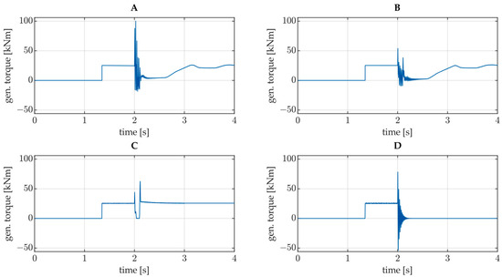
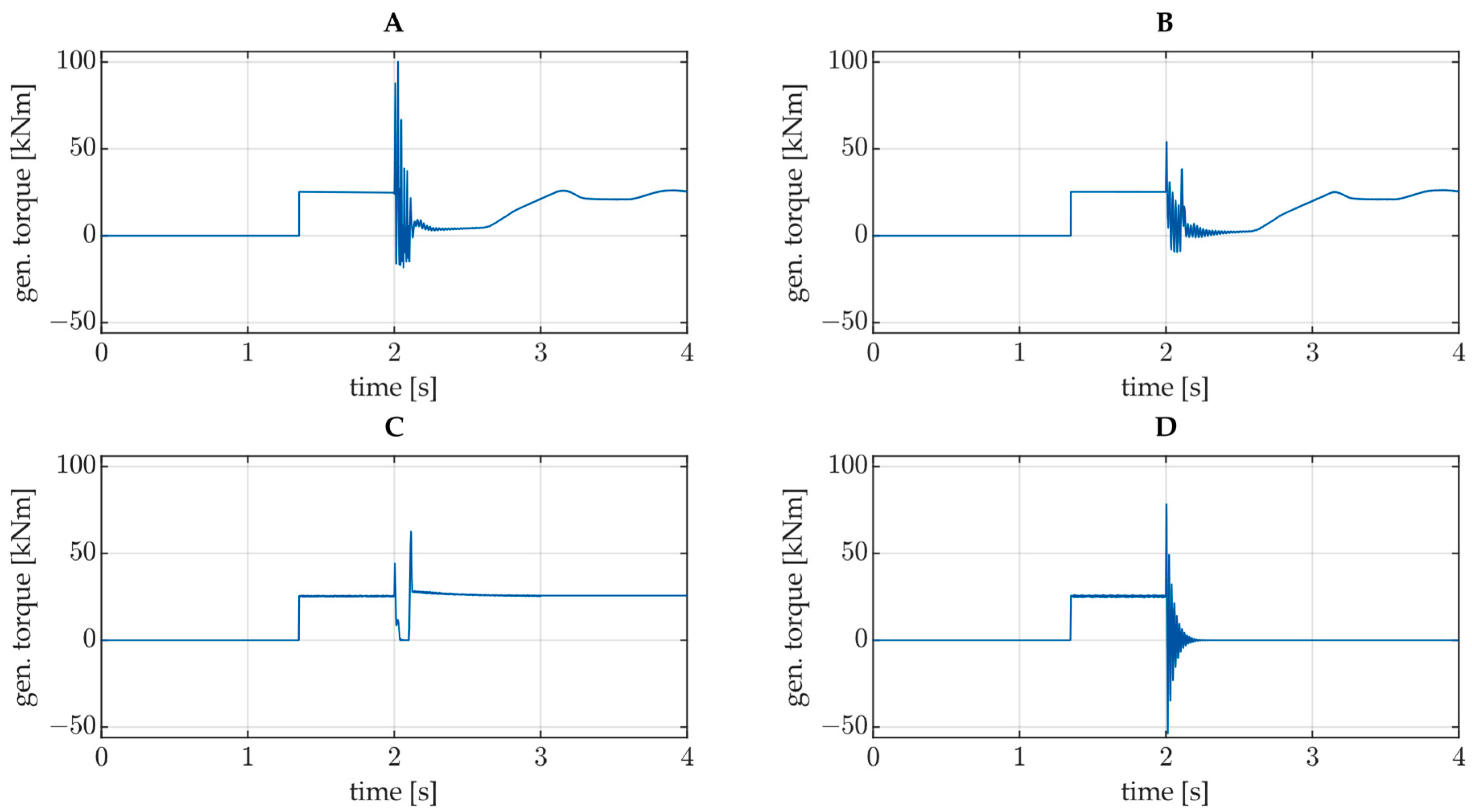
The results of this work are presented in the following. Four different electrical fault load cases are considered in this work. The applied torque at the generator is shown for each load case in Figure 2. Load cases A, B and C are based on grid faults affecting a doubly fed induction generator (DFIG) in a wind turbine with a partial-size power converter. Load case D is caused by a short circuit in the converter of a WT with a single-fed induction generator and a full-size power converter.

Figure 2. Generator torque for each load case: (A) Load case A, (B) Load case B, (C) Load case C, and (D) Load case D.

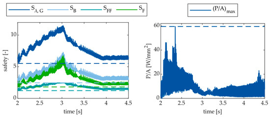
The safety factors of the gear wheels ($S_{\lambda ,G}$, $S_B$, $S_{FF}$, $S_F)$ and the power per loaded area of the bearing (${\left(P/A\right)}_{max}$) are defined as the objectives for the optimization. The safety factors for the gear wheels are most critical immediately after the start of each fault [4]. In Figure 3 on the left, the progression of the values over time for load case A is shown. The fault starts at t = 2 s.

Figure 3. Progression of the objectives for load case A immediately after the fault occurs.

The power per loaded area also shifts to a more critical range immediately after the fault is initiated (on the right in Figure 3). However, individual outliers can be identified, meaning that singular values lead to a high ${\left(P/A\right)}_{max}$.

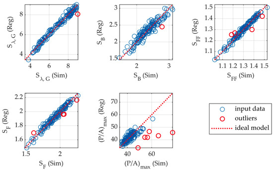
Five regression models are created for the objectives. The robust regression method is used. Apart from the model for ${\left(P/A\right)}_{max}$, a high model quality of $R_{adj}^2\ge 0.875$ is achieved for all models. As illustrated by the values for $R_{adj}^2$, in Table 3, for all four load cases, the regression models deviate significantly more from the simulation results for ${\left(P/A\right)}_{max}$. This is because individual peaks in ${\left(P/A\right)}_{max}$ have a significant impact on the target value, as can be seen in Figure 3.

Table 3. Values of $R_{adj}^2$ for the objectives. High model quality is marked in green, and poor model quality is marked in red.

Load Case	${\mathit{S}}_{\mathit{\lambda },\mathit{G}}$	${\mathit{S}}_{\mathit{B}}$	${\mathit{S}}_{\mathit{F}\mathit{F}}$	${\mathit{S}}_{\mathit{F}}$	${\left(\mathit{P}\mathsf{/}\mathit{A}\right)}_{\mathit{m}\mathit{a}\mathit{x}}$
A	0.977	0.895	0.967	0.963	0.630
B	0.978	0.883	0.972	0.970	0.546
C	0.977	0.901	0.977	0.981	0.258
D	0.977	0.875	0.942	0.936	0.871

In Figure 4, the deviation of the regression models (Reg) from the simulation results (Sim) is shown for the five objectives in the first load case (A). The dashed line shows the course of an ideal regression model for comparison. The outliers that were neglected for model creation are shown in red. Outliers are identified as described in Section 2.4 and they are given lower weights when the regression models are created.

Figure 4. Prediction of regression models compared with simulation results.

A few outliers are detected for $S_{\lambda ,G}$, $S_B$, $S_{FF}$ and $S_F$, and these are close to the other data points. Extreme outliers are only detected for (${P/A)}_{max}$. For these outliers, the simulation model produces significantly worse results than the regression model predicts. The deviation here is up to over 60%. This confirms the lower model quality expected based on the values for $R_{adj}^2$ in Table 3. Overall, it is more difficult to predict the power per loaded area than the other objectives. Nevertheless, the optimization method must select a combination of factors that improves all objectives. Therefore, several Pareto-optimal solutions are considered at each step to filter out incorrect surrogate model predictions.

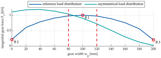
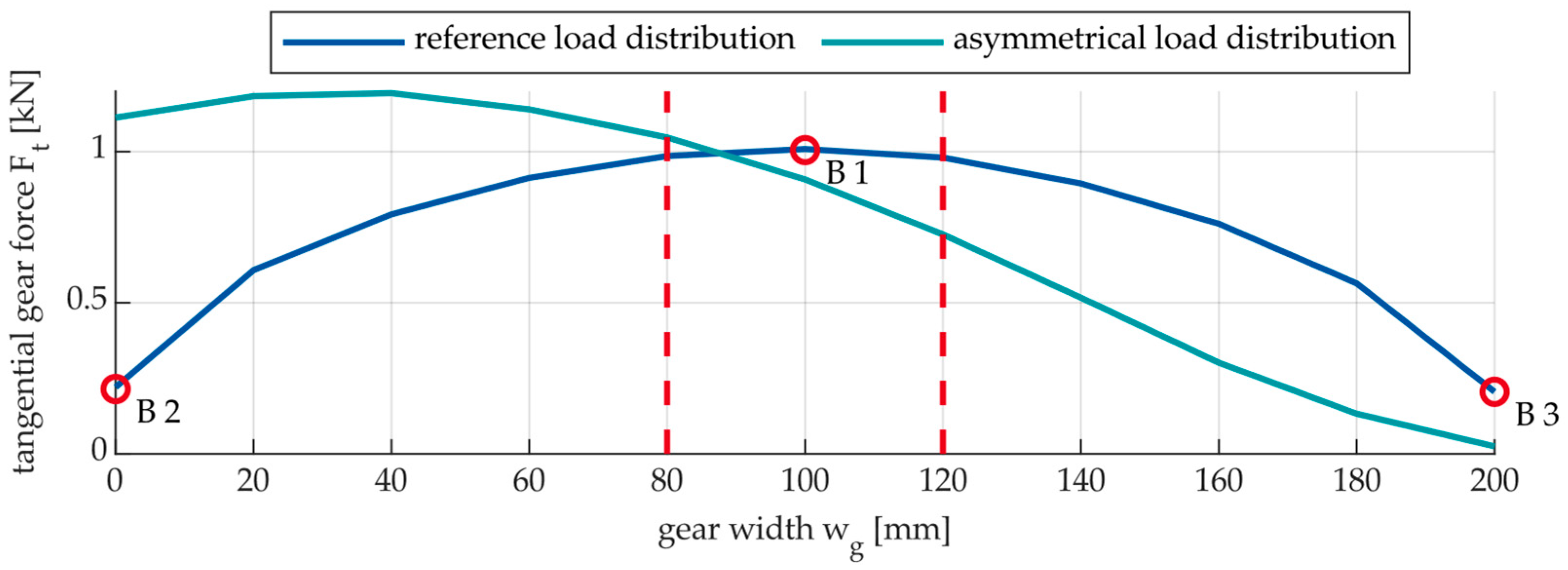
Initial investigations have shown that, depending on the parameter settings, the teeth of the spur gear can tilt in the gear wheels between HSS and IMS. This tilting results in an asymmetrical load distribution of the tangential force F_t across the width w_g of the gear tooth (Figure 5).

Figure 5. Gear tooth load distribution of the reference geometry compared to an asymmetrical gear tooth load distribution.

To avoid such tilting in the optimized design, three constraints (B1–B3) that describe the load distribution are introduced:

• $w_g\left(F_{t,max}\right)\in [80;120]$.
• ${\displaystyle \frac{F_t(w_g=0)}{F_{t,max}}}\le 0.75$.
• ${\displaystyle \frac{F_t(w_g=200)}{F_{t,max}}}\le 0.75$.

These three constraints ensure that the tooth flank is loaded centrally. Similar to the objectives, regression models are created for these constraints to include them in the optimization procedure.

For $S_{\lambda }$, $S_B$, $S_{FF}$ and $S_F$, it is further specified that all optimized safeties need to be higher than the corresponding reference ($S_i\ge S_{i,ref}$). Another constraint is that ${\left(P/A\right)}_{max}\le {\left(P/A\right)}_{max,ref}$. With these constraints, the optimization is performed using the regression models created. The result of the optimization is 325,000 Pareto-optimal solutions per load case. The best ten solutions per load case are selected based on the $Q_{tot,I}$ quality criterion. These solutions are then validated by simulations using the MBS model. Then, the simulation results are used to reevaluate these solutions using the $Q_{tot,II}$ criterion. Table 4 lists the three best Pareto-optimal solutions for each load case (A, B, C and D).

Table 4. Objective values of the best three solutions per load case.

ID	$\frac{{\mathit{S}}_{\mathit{\lambda }}}{{\mathit{S}}_{\mathit{\lambda },\mathit{r}\mathit{e}\mathit{f}}}$	$\frac{{\mathit{S}}_{\mathit{B}}}{{\mathit{S}}_{\mathit{B},\mathit{r}\mathit{e}\mathit{f}}}$	$\frac{{\mathit{S}}_{\mathit{F}\mathit{F}}}{{\mathit{S}}_{\mathit{F}\mathit{F},\mathit{r}\mathit{e}\mathit{f}}}$	$\frac{{\mathit{S}}_{\mathit{F}}}{{\mathit{S}}_{\mathit{F},\mathit{r}\mathit{e}\mathit{f}}}$	$\frac{{\left(\mathbf{P}\mathsf{/}\mathbf{A}\right)}_{\mathit{m}\mathit{a}\mathit{x}}}{{\left(\mathit{P}\mathsf{/}\mathit{A}\right)}_{\mathit{m}\mathit{a}\mathit{x},\mathit{r}\mathit{e}\mathit{f}}}$	${\mathit{Q}}_{\mathit{t}\mathit{o}\mathit{t},\mathit{I}\mathit{I}}$
A1	128%	131%	131%	133%	85%	1.268
A2	124%	136%	132%	135%	87%	1.267
A3	128%	130%	130%	133%	85%	1.262
B1	133%	135%	135%	139%	96%	1.246
B2	145%	119%	135%	139%	95%	1.235
B3	136%	125%	134%	137%	96%	1.229
C1	135%	131%	130%	132%	100%	1.197
C2	130%	136%	130%	132%	101%	1.196
C3	125%	138%	129%	132%	103%	1.192
D1	131%	125%	126%	128%	86%	1.227
D2	132%	126%	127%	129%	88%	1.226
D3	132%	125%	127%	129%	93%	1.201

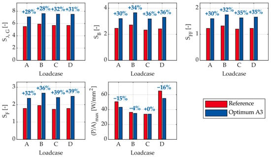
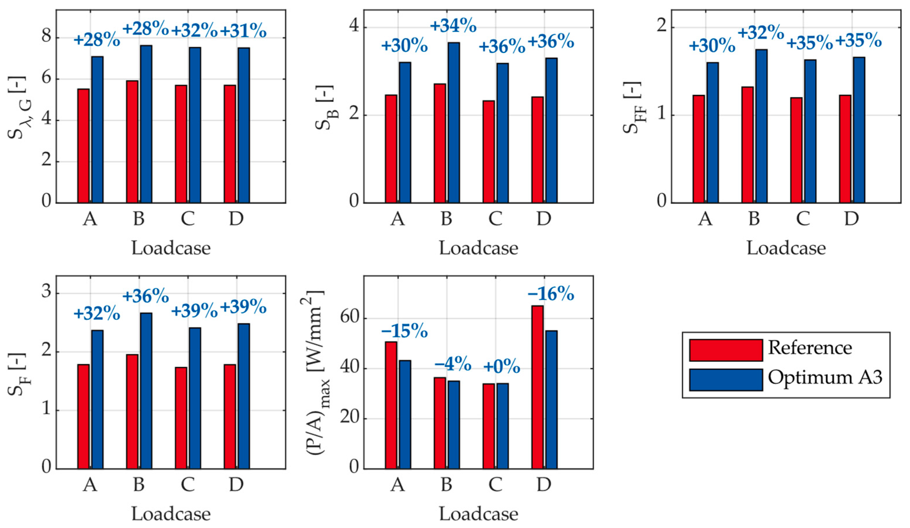
The three best solutions for load case A are chosen for further evaluation. To find a solution that improves the objectives for all four load cases, the factor settings of solutions A1, A2 and A3 are simulated with all four load cases. As only one of those three solutions improves all the objectives for all four load cases, this solution (A3) is selected. The resulting objectives are shown in Figure 6. The value of each objective is shown in blue for each of the four load cases. The respective reference value with default settings is shown in red.

Figure 6. Improvement of the objectives using the optimization procedure.

With this parameter configuration, an increase of at least 28% in the four safety factors of the gear wheels ($S_{\lambda ,G}$, $S_B$, $S_{FF}$ and $S_F$) can be achieved. Additionally, ${\left(P/A\right)}_{max}$ improves by at least 4% for three of the four load cases. For load case C, however, ${\left(P/A\right)}_{max}$ remains almost unchanged. The limitations of the method are evident in the optimization of the P/A ratio of the cylindrical rolling element bearing. Depending on the load case, this indicates that no significant improvement in P/A can be achieved by varying the parameters within the defined limits.

A comparison with the values from Table 5 shows that, depending on the load case, the selected optimum A3 achieves equal or up to 2% better values for ${\left(P/A\right)}_{max}$ and a maximum 4% lower improvement in the safety factors of the gear stage compared to the respective load case optimization. It can be seen that the optimization for single load cases did not always result in the best solution. For load cases C and D, solution A3 leads to better objective values than solutions C1 and D1. No better solution was found for the individual optimization for load cases C and D compared to the solution A3 due to the deviation between the regression model and the MBS model. Nonetheless, it can be stated that optimizing the microgeometry of the HSS components for a single critical electrical fault is sufficient to achieve a similarly higher robustness of the gearbox than for an optimization considering multiple electrical load cases. Optimizing for a single fault load case does not necessarily lead to the best result. However, optimizing for a single load case (in this case, load case A) results in significantly greater robustness for multiple fault load cases simultaneously.

Table 5. Objectives of the best solution per load case compared to the common solution A3 (bold).

Load Case	ID	$\frac{{\mathit{S}}_{\mathit{\lambda }}}{{\mathit{S}}_{\mathit{\lambda },\mathit{r}\mathit{e}\mathit{f}}}$	$\frac{{\mathit{S}}_{\mathit{B}}}{{\mathit{S}}_{\mathit{B},\mathit{r}\mathit{e}\mathit{f}}}$	$\frac{{\mathit{S}}_{\mathit{F}\mathit{F}}}{{\mathit{S}}_{\mathit{F}\mathit{F},\mathit{r}\mathit{e}\mathit{f}}}$	$\frac{{\mathit{S}}_{\mathit{F}}}{{\mathit{S}}_{\mathit{F},\mathit{r}\mathit{e}\mathit{f}}}$	$\frac{{\left(\mathbf{P}\mathsf{/}\mathbf{A}\right)}_{\mathit{m}\mathit{a}\mathit{x}}}{{\left(\mathit{P}\mathsf{/}\mathit{A}\right)}_{\mathit{m}\mathit{a}\mathit{x},\mathit{r}\mathit{e}\mathit{f}}}$
B	B1	133%	135%	135%	139%	96%
	A3	129%	135%	132%	136%	96%
C	C1	135%	131%	130%	132%	100%
	A3	132%	137%	136%	139%	100%
D	D1	131%	125%	126%	128%	86%
	A3	132%	136%	135%	139%	84%
${\Delta }_{min}$		−4%	−0%	−0%	−3%	−2%
${\Delta }_{max}$		+1%	+11%	+9%	+11%	+0%

Based on this, it can be concluded that only one load case is needed to create surrogate models for optimizing the gearbox. Therefore, the computational effort required for optimizing for several electrical faults can be significantly reduced. Only validation of the results is carried out with all load cases considered. The parameter settings for the chosen optimum A3 are listed in Table 6 (the meanings of parameter abbreviations can be found in Table 2).

Table 6. Parameter configuration of ID A3.

	${\mathit{C}}_{\mathit{a},\mathit{H}\mathit{S}\mathit{S}}$	${\mathit{C}}_{\mathit{a},\mathit{I}\mathit{M}\mathit{S}}$	${\mathit{C}}_{\mathit{\alpha },\mathit{H}\mathit{S}\mathit{S}}$	${\mathit{C}}_{\mathit{\alpha },\mathit{I}\mathit{M}\mathit{S}}$	${\mathit{I}}_{\mathit{e},\mathit{I}\mathit{M}\mathit{S}}$	${\mathit{b}}_{\mathit{e},\mathit{I}\mathit{M}\mathit{S}}$	${\mathit{C}}_{\mathit{b},\mathit{H}\mathit{S}\mathit{S}}$	${\mathit{C}}_{\mathit{b},\mathit{I}\mathit{M}\mathit{S}}$	${\mathit{f}}_{\mathit{H}\mathit{\beta },\mathit{H}\mathit{S}\mathit{S}}$	${\mathit{f}}_{\mathit{H}\mathit{\beta },\mathit{I}\mathit{M}\mathit{S}}$	${\mathit{x}}_{\mathit{H}\mathit{S}\mathit{S}}$	${\mathit{c}}_{\mathit{R}}$
	[$\mathsf{\mu }\mathbf{m}$]	[$\mathsf{\mu }\mathbf{m}$]	[$\mathsf{\mu }\mathbf{m}$]	[$\mathsf{\mu }\mathbf{m}$]	[$\mathsf{\mu }\mathbf{m}$]	[$\mathbf{m}\mathbf{m}$]	[$\mathsf{\mu }\mathbf{m}$]	[$\mathsf{\mu }\mathbf{m}$]	[$\mathbf{m}\mathbf{r}\mathbf{a}\mathbf{d}$]	[$\mathbf{m}\mathbf{r}\mathbf{a}\mathbf{d}$]	[$\mathbf{-}$]	[$\mathsf{\mu }\mathbf{m}$]
Reference	40.00	30.0	20.00	0.00	25.00	35.00	50.00	0.00	0.11	0.11	0.11	117.5
ID A3	55.59	112.1	23.26	93.92	49.73	4.24	0.38	6.98	0.04	0.16	0.20	90.13

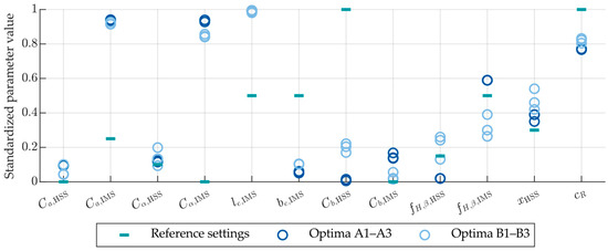
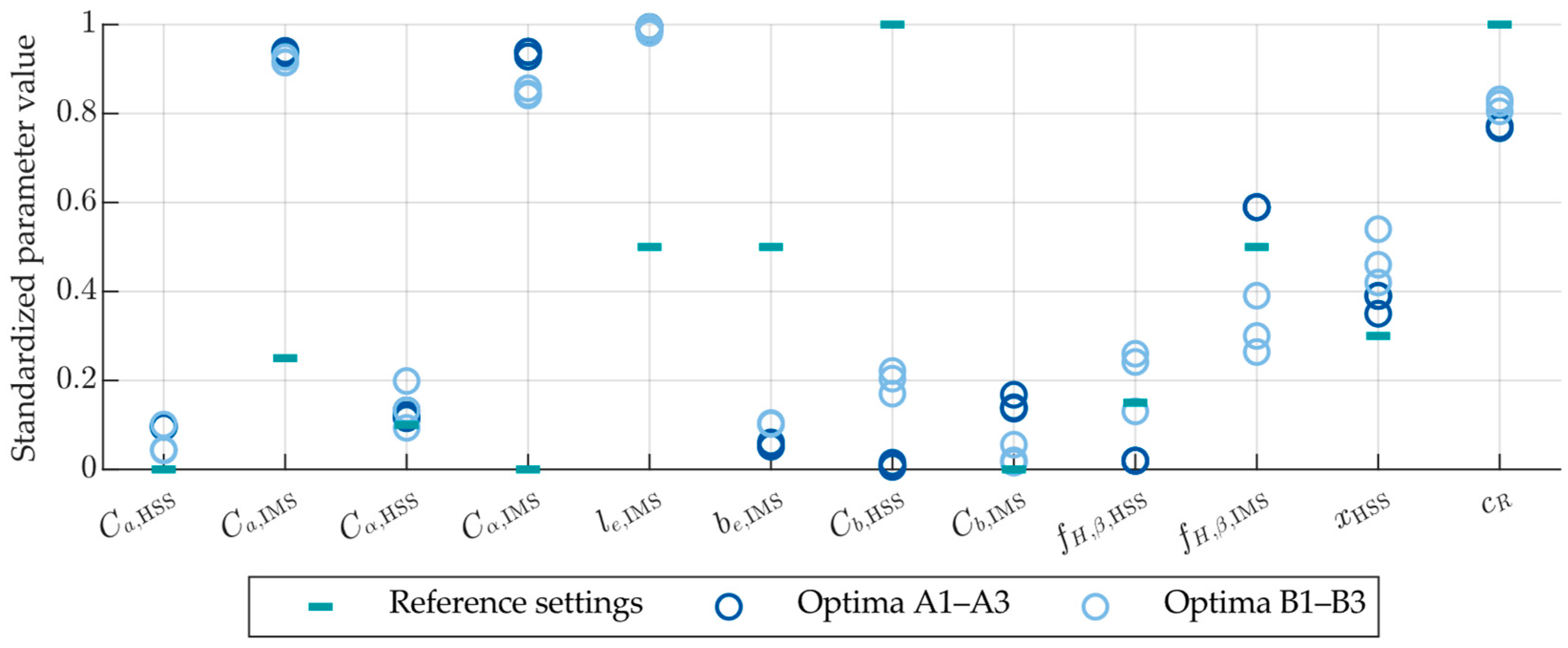
To estimate how the parameters should be changed, Figure 7 shows the parameter settings for solutions A1–A3 and B1–B3 in standardized form, together with the reference settings. Compared to the reference parameter configuration, an increase in the profile shift coefficient ($x_{HSS}$) is recommended. Moreover, higher values for the tip relief of both gears ($C_{a,HSS}$ and $C_{a,IMS}$) have a positive impact on the objectives. While the profile crowning of the HSS gear ($C_{\alpha ,HSS}$) remains largely unchanged, the corresponding modification of the IMS gear ($C_{\alpha ,IMS}$) should be increased. For the IMS gear, a larger end relief ($I_{e,IMS}$) combined with a reduced end relief width ($b_{e,IMS}$) is recommended. The flank line crowning of the HSS gear ($C_{b,HSS}$) should be reduced and of the IMS gear ($C_{b,IMS}$) should be increased. Based on Figure 7, no clear trend for the flank line slope modifications ($f_{H\beta ,HSS}$ and $f_{H\beta ,IMS}$) can be determined. The rolling element bearing should be designed with reduced clearance ($c_R$).

Figure 7. Standardized parameter settings for Optima A1–A3 and B1–B3.

4. Conclusions and Outlook

This study determined an optimized gearbox design considering four different electrical special load cases which are not considered in current design standards yet. Electrical fault load cases that are critical for gearbox robustness were taken into consideration. The focus was on the gear wheels of the HSS and IMS, as well as the HSS’s floating cylindrical roller bearing, where damage often occurs. An efficient test plan was created. The quality of the test plan was ensured by correlating the factor combinations. Computationally efficient regression models of the objectives were created to be used in a mathematical optimization procedure.

All objective values were improved compared to the reference design of the gearbox. The safety factors for damage to the gear wheels between HSS and IMS increased by at least 28%. The power per loaded area in the floating bearing was also reduced, but only minimally, depending on the fault load case under consideration. Overall, a higher robustness of the gearbox against the damage criteria can be determined for all four considered electrical fault load cases. Optimizing the gearbox microgeometry for one electrical fault is sufficient to significantly increase robustness against several electrical faults. Consequently, the computational effort required for MBSs can be reduced by approximately 75% (compared to using four load cases for the optimization).

The limitations of the method were also identified. As the results show, the optimization of the microgeometry of the cylindrical roller bearing only decreases the risk of damage slightly. Since the HSS bearings fail, in future studies, the cylindrical roller bearing will be replaced with a journal bearing. The implementation of the journal bearing will be investigated in more detail and included in the optimization procedure. Journal bearings are, in general, not susceptible to the peak loads resulting from the torque ripples during electrical faults.

References

- Bundesministerium für Wirtschaft und Energie. Climate Action Plan 2050: Principles and Goals of the German Government’s Climate Policy. Available online: https://www.bundeswirtschaftsministerium.de/Redaktion/DE/Publikationen/Industrie/klimaschutzplan-2050.pdf?__blob=publicationFile&v=1 (accessed on 30 July 2025).
- Dao, C.; Kazemtabrizi, B.; Crabtree, C. Wind turbine reliability data review and impacts on levelised cost of energy. Wind Energy 2019, 22, 1848–1871. [Google Scholar] [CrossRef] [Scilit]
- Röder, J.; Jacobs, G.; Bosse, D.; Izal, J.L.R. Reduction of gearbox loads of a DFIG wind turbine during grid faults with optimized converter configurations. J. Phys. Conf. Ser. 2022, 2265, 32034. [Google Scholar] [CrossRef] [Scilit]
- Bußkamp, P.; Jacobs, G.; Röder, J. Multiobjective wind turbine gearbox design optimization to reduce component damage risk during grid faults. Forsch. Ingenieurwesen 2025, 89, 48. [Google Scholar] [CrossRef] [Scilit]
- Matzke, D.; Schelenz, R.; Reisch, S.; Roscher, B.; Jacobs, G.; Theling, J.; Schroers, M.; Löpenhaus, C.; Brecher, C. Validation of the gearbox load calculation of a wind turbine MBS model. In Conference for Wind Power Drives, CWD 2019, Conference Proceedings, Aachen, Germany, 12–13 March 2019; Abel, D., Brecher, C., de Doncker, R.W., Eds.; Books on Demand: Norderstedt, Germany, 2019; p. 62025. ISBN 9783748178675. [Google Scholar]
- Matzke, D.; Jacobs, G.; Schelenz, R. Full scale system simulation of a 2.7 MW wind turbine on a system test bench. In Conference for Wind Power Drives, CWD 2017, Conference proceedings, Aachen, Germany, 7–8 March 2017; Werkmeister, A.T., Abel, D., Brecher, C., de Doncker, R.W., Hameyer, K., Jacobs, G., Monti, A., Schröder, W., Eds.; BoD—Books on Demand: Norderstedt, Germany, 2017; ISBN 9783743134560. [Google Scholar]
- Forschungsvereinigung Antriebstechnik e.V. FVA-Gondel: Belastungen an den Antriebskomponenten von Winenergieanlagen; Research Project No. 730; Final Report; Forschungsvereinigung Antriebstechnik e.V.: Frankfurt am Main, Germany, 2019. [Google Scholar]
- Kiekbusch, T. Zylinderrollenlagermodul für Simpack, FVA Forschungsvorhaben Nr. 625 II: Final Report 1234; Forschungsvereinigung Antriebstechnik e.V.: Frankfurt am Main, Germany, 2017. [Google Scholar]
- DIN ISO 6336-22; Calculation of Load Capacity of Spur and Helical Gears—Part 22: Calculation of Micropitting Load Capacity. International Organization for Standardization: Geneva, Switzerland, 2018.
- DIN ISO 6336-20; Calculation of Load Capacity of Spur and Helical Gears—Part 20: Calculation of Scuffing Load Capacity—Flash Temperature Method. International Organization for Standardization: Geneva, Switzerland, 2022.
- DIN ISO 6336-4; Calculation of Load Capacity of Spur and Helical Gears—Part 4: Calculation of Tooth Flank Fracture Load Capacity. International Organization for Standardization: Geneva, Switzerland, 2019.
- DIN ISO 6336-3; Calculation of Load Capacity of Spur and Helical Gears—Part 3: Calculation of Tooth Bending Strength. International Organization for Standardization: Geneva, Switzerland, 2019.
- Forschungsvereinigung Antriebstechnik e.V. Schädlicher Wälzlagerschlupf: Wann ist Wälzlagerschlupf schädlich und führt zum Ausfall des Wälzlagers? Research Project No. 663 I; Final Report; Forschungsvereinigung Antriebstechnik e.V.: Frankfurt am Main, Germany, 2015. [Google Scholar]
- Siebertz, K.; van Bebber, D.; Hochkirchen, T. Statistische Versuchsplanung: Design of Experiments (DoE), 2nd ed.; Springer: Berlin/Heidelberg, Germany, 2017; ISBN 978-3-662-55743-3. [Google Scholar]
- MathWorks. MATLAB R2022b, MathWorks: Natick, MA, USA, 2022.
Disclaimer/Publisher’s Note: The statements, opinions and data contained in all publications are solely those of the individual author(s) and contributor(s) and not of MDPI and/or the editor(s). MDPI and/or the editor(s) disclaim responsibility for any injury to people or property resulting from any ideas, methods, instructions or products referred to in the content. |
© 2026 by the authors. Licensee MDPI, Basel, Switzerland. This article is an open access article distributed under the terms and conditions of the Creative Commons Attribution (CC BY) license.