Addressing Data Sparsity in EV Charging Load Forecasting: A Novel Zero-Inflated Neural Network Approach

Abstract

Accurate electric vehicle (EV) charging load forecasting is essential for grid planning and resource allocation, yet existing approaches struggle with the inherent sparsity of charging data—a phenomenon characterized by excessive zeros representing periods of no charging activity. This paper addresses this challenge through a novel framework combining a Zero-Inflated Neural Network (ZINN) architecture with an Evolutionary Neural Architecture Search (ENAS) algorithm. ZINN explicitly decomposes the forecasting problem into binary classification (predicting charging occurrence) and regression (estimating energy magnitude conditioned on occurrence), enabling the model to learn distinct patterns for the absence and presence of charging events. Rather than relying on manually designed architectures, ENAS automatically discovers optimal encoder and decoder configurations from a comprehensive search space encompassing modern architectures (LSTM, GRU, Transformer, and iTransformer), layer configurations, activation functions, and hyperparameters. The evolutionary algorithm balances prediction accuracy with computational efficiency through multi-objective optimization. Extensive experiments on real-world EV charging data from 30 stations in Wuhan demonstrate that the ZINN+ENAS framework achieves the lowest prediction error compared to conventional baselines, with the discovered optimal configuration substantially outperforming hand-crafted designs. Comprehensive ablation studies reveal that the asymmetric dual-head architecture and adaptive regularization strategies are critical for handling data sparsity. These findings highlight the importance of explicit zero-inflation modeling and automated architecture discovery for specialized forecasting tasks, providing practitioners with an open-source framework for practical EV charging load prediction.

1. Introduction

The rapid proliferation of electric vehicles (EVs) is fundamentally transforming the landscape of transportation and energy consumption. As reported by the International Energy Agency (IEA), global EV sales reached nearly 14 million in 2023, and this trend is projected to continue as governments worldwide intensify their efforts to promote greener technologies [1,2]. This growth necessitates the development of efficient electricity supply infrastructure capable of supporting increasing charging demands. Accurately forecasting EV charging loads is critical for effective energy management and grid stability [3]. Understanding the intricacies of charging behaviors is vital, as they can vary significantly based on several factors, including location, time of day, and user patterns [4].

One of the main challenges in integrating EV charging infrastructure into existing energy systems is the inherently sparse nature of charging demand data. Many EV charging stations experience periods of low utilization, leading to sparse training data that complicates accurate load forecasting. The uneven distribution of EVs across various charging stations results in frequent empty charging sessions, where infrequently utilized stations may remain vacant for extended periods. This zero-inflated characteristic of the data—where the distribution exhibits an excess of zero values compared to a standard continuous distribution—significantly undermines the reliability of conventional forecasting models. Consequently, the lack of sufficient historical usage data complicates the optimization of energy distribution networks aimed at accommodating fluctuating demand.

EV charging load patterns exhibit significant temporal variability at multiple scales: diurnal cycles driven by work commute patterns, weekly patterns reflecting different usage behaviors on weekends versus weekdays, and seasonal variations influenced by climate and travel patterns. Simultaneously, the heterogeneity of charging environments introduces substantial spatial variability, as each station exhibits distinct usage patterns influenced by various contextual factors such as proximity to commercial centers, residential areas, or transportation hubs. This multi-scale temporal-spatial heterogeneity poses a fundamental challenge for conventional forecasting approaches that assume stationary distributions or homogeneous patterns across all locations.

While deep learning techniques such as Long Short-Term Memory (LSTM) networks [5] and Transformer [6] have been widely adopted to improve prediction accuracy over traditional statistical methods, they often struggle to effectively handle zero values and the distributional characteristics of sparse data. This fundamental limitation arises from three key factors: (1) standard regression models optimize for mean squared error, which is dominated by abundant zero observations and systematically underestimates charging probabilities; (2) traditional neural architectures lack explicit mechanisms to model the zero-inflation component, treating all predictions uniformly regardless of whether they represent charging or non-charging periods; and (3) manually designed architectures are not adaptive to the unique sparsity patterns of EV charging data, resulting in suboptimal feature learning for both occurrence and magnitude prediction.

To address the multifaceted challenges of data sparsity and complex temporal patterns in EV charging load forecasting, we propose an integrated framework combining two key innovations: First, a novel Zero-Inflated Neural Network (ZINN) architecture is introduced, specifically designed to handle the sparse nature of EV charging data. Second, an automated Evolutionary Neural Architecture Search (ENAS) framework discovers optimal encoder and decoder configurations within a comprehensive search space.

The main contributions of this work are as follows:

1.

Novel Zero-Inflated Neural Network (ZINN) Architecture: We introduce a dual-component ZINN that explicitly tackles the zero-inflation problem inherent in EV charging data. By decomposing forecasting into binary classification (presence/absence of charging) and regression (magnitude of energy consumption), ZINN yields more accurate and interpretable predictions than standard regression. It features adaptive loss weighting and instance normalization to handle station heterogeneity.

2.

Automated Evolutionary Neural Architecture Search (ENAS) Framework: We develop an ENAS framework using evolutionary algorithms to automatically discover optimal neural network configurations for EV charging load forecasting. This approach systematically explores a rich search space and incorporates multi-objective optimization to balance prediction accuracy with model efficiency, overcoming limitations of manual design.

3.

Comprehensive Empirical Validation: Extensive experiments on real-world EV charging data from 30 stations demonstrate that our ZINN+ENAS framework significantly outperforms conventional baselines.

The remainder of this paper is organized as follows. Section 2 reviews related work in time series forecasting, zero-inflated modeling, and neural architecture search. The data exploration and preprocessing section is then presented in Section 3, followed by the problem formulation in Section 4. Section 5 presents the proposed ZINN architecture and the evolutionary NAS framework in detail. Section 6 describes the experimental setup, datasets, and results, including comparisons with baseline methods and ablation studies. Finally, Section 7 concludes the paper and outlines future directions.

2. Related Work

The accurate prediction of EV charging demand has gained considerable attention with the growing prevalence of electric vehicles. The increasing need for effective forecasting methods is driven by challenges associated with the limited availability of charging infrastructure and the demand for efficient energy management in urban settings [3,7]. One essential aspect of forecasting EV charging demand lies in integrating diverse data sources, including historical charging patterns, traffic conditions, environmental influences and efficiency of electric vehicle charging stations [8]. Studies have demonstrated that employing big data technologies and advanced algorithms can significantly enhance the accuracy of predictions and address complexities associated with charging behaviors [9,10].

2.1. Traditional Forecasting Methods

Traditionally, EV charging demand prediction has relied heavily on statistical models and rule-based algorithms. Techniques such as Auto-Regressive Integrated Moving Average (ARIMA) [11], exponential smoothing [12], and regression analysis have been commonly employed to estimate future charging loads. However, these methodologies often encounter challenges associated with data sparsity, as a result of infrequent charging in certain regions. Because a large fraction of historical records may correspond to near-zero (or zero) loads, regression-oriented objectives (e.g., MSE) tend to bias predictions toward underestimating charging occurrences and magnitudes. In addition, the number of active stations and their utilization rates further affect the availability and balance of informative samples, which poses barriers to robust and accurate forecasting [13]. In response to these limitations, recent advances have seen a shift toward machine learning methods, which incorporate ensemble techniques and hybrid approaches that combine statistical and machine learning methodologies [14,15,16]. Despite these developments, issues related to the quality and sparsity of data continue to hinder the accuracy of load forecasting models.

2.2. Deep Learning Approaches for Time Series Forecasting

Recently, deep learning-based approaches have gained significant traction in the realm of time series forecasting and EV charging demand prediction. Recurrent neural networks, particularly Long Short-Term Memory (LSTM) networks [5] and Gated Recurrent Units (GRU) [17], have shown great promise in capturing temporal dependencies and have outperformed traditional statistical methods across several studies [18,19,20,21,22]. These architectures excel at modeling sequential patterns through their gating mechanisms, which control information flow and help mitigate the vanishing gradient problem.

Additionally, transformer architectures [6] have emerged as a powerful alternative for time series forecasting, demonstrating superior performance in capturing long-range dependencies. Recent innovations such as iTransformer [23] have introduced an inverted architecture that treats time series variables as tokens, achieving state-of-the-art results on multiple forecasting benchmarks [24]. These transformer-based approaches offer improved parallelization and attention mechanisms that enable more efficient learning of complex temporal patterns compared to recurrent approaches.

2.3. Zero-Inflated Modeling

Handling sparse and zero-inflated data remains a critical challenge in many real-world forecasting applications. Zero-inflated models, originally developed in statistical literature [25,26], decompose the problem into two components: a binary model for predicting the occurrence of non-zero values and a regression model for predicting magnitudes conditioned on occurrence. These approaches have been successfully adapted for count data and sparse time series [27,28]. However, the integration of zero-inflated modeling with deep neural networks remains relatively unexplored in the EV charging forecasting literature.

Our proposed ZINN bridges classical zero-inflated modeling and modern deep learning by maintaining the interpretable two-component structure while leveraging neural networks to learn flexible, non-parametric mappings from features to both occurrence probabilities and magnitudes. This hybrid approach enables superior performance on sparse time series compared to purely parametric or purely neural methods.

2.4. Neural Architecture Search

Neural Architecture Search (NAS) has become an increasingly important methodology for automating the design of neural networks, moving away from manual architecture engineering. Early NAS approaches employed reinforcement learning to guide architecture search [29], while more recent methods have adopted evolutionary algorithms [30], Bayesian optimization [31], and differentiable search methods [32]. Evolutionary NAS approaches have demonstrated particular promise for complex search spaces, efficiently exploring architectures through mutation and crossover operators to discover novel architectural patterns [33].

The benefits of NAS are multifaceted: automated architecture search can discover non-intuitive designs that outperform hand-crafted architectures, adapt to task-specific characteristics, and improve both accuracy and computational efficiency. However, most existing NAS work focuses on standard classification or regression tasks such as image classification, with fewer studies addressing the unique challenges of sparse time series forecasting [34]. The application of NAS to specialized problems such as zero-inflated forecasting with dual-component architectures remains largely unexplored. This gap represents an opportunity to leverage automated architecture discovery to find optimal configurations specifically tailored for sparse EV charging load prediction, where the interplay between encoder design, activation functions, regularization strategies, and loss weighting is critical for performance.

2.5. Identified Research Gaps

Despite considerable progress in EV charging demand forecasting, persistent challenges remain. First, existing methods largely depend on the quality and quantity of available data, with data sparsity continuing to limit predictive accuracy in many regions. Second, there is a notable gap in methodologies that effectively combine zero-inflation handling with modern deep learning architectures and automated architecture discovery. Third, while extensive research exists on deterministic architecture design for general time series forecasting, the application of automated architecture search to sparse forecasting problems with specific structural characteristics remains underexplored. Fourth, most existing approaches treat architecture design as a one-time decision rather than adapting architectures to specific data characteristics, forecasting horizons, or station-specific patterns. Finally, the trade-off between model accuracy and computational efficiency—particularly important for resource-constrained deployment scenarios—has not been systematically addressed in the context of zero-inflated forecasting. This work addresses these gaps by proposing an integrated framework that combines zero-inflated neural networks with evolutionary architecture search, enabling automated discovery of optimal architectures for sparse EV charging forecasting tasks while maintaining computational efficiency.

3. Data Source

We conducted our analysis using real-world EV charging data collected in Wuhan from January to May 2018. The dataset comprises detailed records of individual charging sessions, including temporal information (start and end times) and spatial locations, extracted from comprehensive EV trajectory records. These trajectory records capture the full spectrum of EV user behaviors—including travel, parking, and charging patterns—enabling analysis of both the temporal dynamics and spatial heterogeneity inherent in urban EV charging demand.

We first clustered the geographic coordinates of charging sessions to derive a set of charging stations. Each charging session provides both a start location and an end location. In our implementation, we use the start coordinates as the representative station location. Specifically, we: (i) drop sessions with missing GPS coordinates; (ii) detect invalid start coordinates (latitude or longitude $\le 0$ or NaN) and replace the invalid start coordinates with the corresponding end coordinates when available; (iii) convert coordinates into radians and compute great-circle distances using the haversine metric.

We then apply DBSCAN clustering with haversine distance to group spatially close sessions into station clusters. The DBSCAN radius parameter is set as ${\epsilon }_{\mathrm{meters}}=100$ m, converted to the haversine angular distance:

$${\epsilon }_{\mathrm{rad}}={\displaystyle \frac{{\epsilon }_{\mathrm{meters}}}{1000}}·{\displaystyle \frac{1}{R_{\mathrm{earth}}}},$$

where $R_{\mathrm{earth}}=6371.0088$ km. We set min_samples = 1 so that even isolated sessions can be assigned a station. Under this setting, DBSCAN may still output noise labels in some cases; if noise points exist, we assign each noise session a unique station ID (i.e., each noise point becomes its own station) to ensure every session has a valid station ID.

After clustering, we identified 30 distinct charging stations. For each station, the dataset summarizes: (i) station coordinates as the mean of the clustered start latitudes and longitudes; (ii) num_sessions, the number of sessions assigned to the station; (iii) num_vehicles, the number of unique vehicles (VINs) observed at the station; (iv) total_energy_kWh, the total consumed energy in kilowatt-hours across all sessions; (v) avg_session_duration_hours, the average session duration in hours; and (vi) the operational time span, captured by the earliest start_time (from late January) and the latest end_time (up to late May).

A summary of key features is presented in Table 1. This summary table highlights the variability among stations in terms of activity levels and energy consumption, which is vital for understanding station-level demand dynamics. It underscores the importance of regional aggregation in the pursuit of accurate demand forecasting.

Table 1. Summary statistics of key features of charging stations in Wuhan.

	Minimum	Maximum	Mean	Median	Standard Deviation
Number of Sessions	1973	45,291	20,000	18,000	9000
Number of Vehicles	7	1016	400	350	200
Total Energy Consumption (kWh)	2399.20	1,000,612.13	300,000	250,000	200,000
Average Session Duration (hours)	0.97	4.53	2.25	2.10	0.60

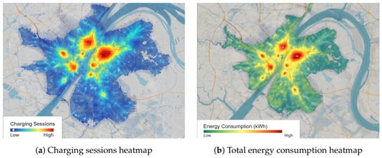
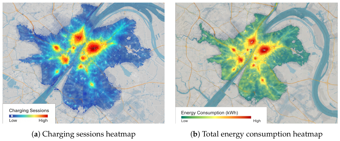
Figure 1 presents regional heatmaps that illustrate the geographic distribution of charging stations in Wuhan: The first heatmap depicts the distribution of charging sessions across various regions, identifying hotspots where the demand for charging is most intense. The second heatmap represents total energy consumption (in kWh) across these regions, revealing areas with significant energy usage for charging.

Figure 1. The heatmap of all charging sessions, left is the charging frequency and right is the charging load.

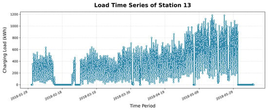
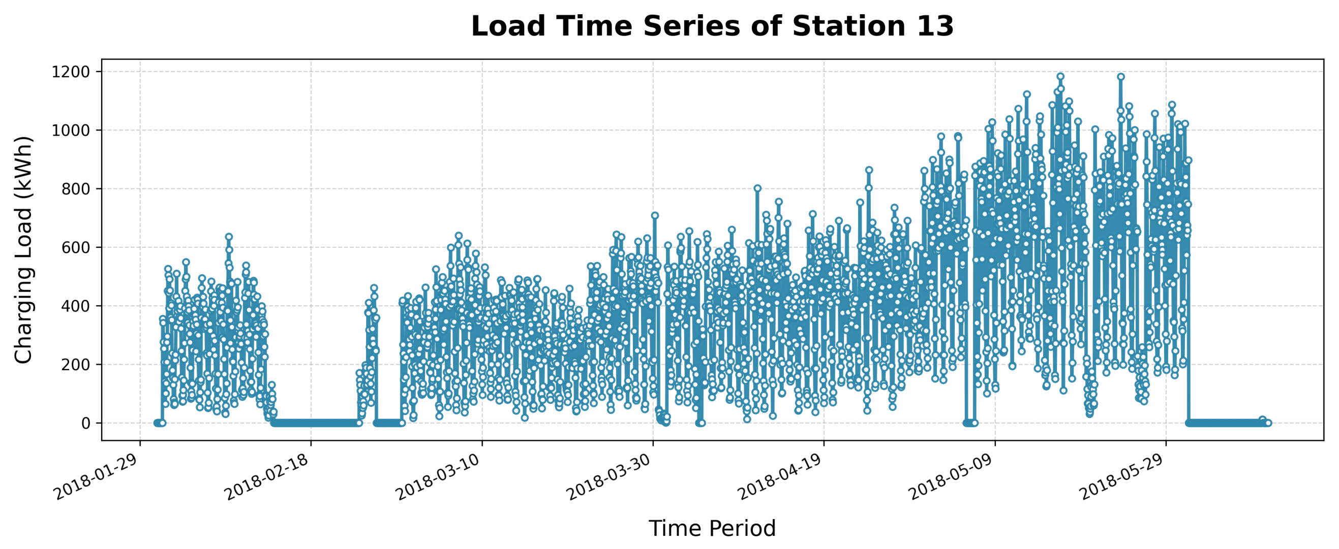
Notably, there is a marked imbalance in charging loads; some stations exhibit high usage frequency across all time intervals while others do not. Taking the load time series of a station shown in Figure 2 as an example, we observe, at least, three time intervals where the load is (near) zero kWh.

Figure 2. Daily charging load for a charging station over a 24 h period, illustrating intraday variation and periods of zero load.

3.1. Sparsity Analysis of Charging Load Data

We have significantly expanded our investigation into the presence and temporal distribution of zero values (periods without recorded charging activity). This enhanced analysis explicitly incorporates daily and weekly seasonality to reveal the intricate relationship between charging inactivity and time structures, providing a more comprehensive understanding of station utilization.

3.2. Overall and Station-Level Sparsity

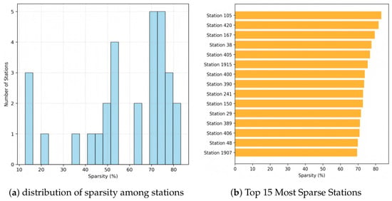
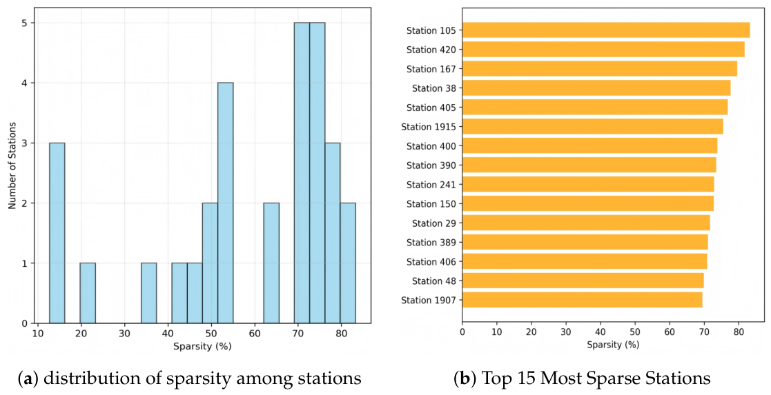
Our data indicates an overall sparsity of 61.2% across all charging records, signifying that a substantial portion of observed periods reflects no charging events. This high degree of sparsity necessitates a detailed examination of its underlying patterns. The distribution of sparsity among individual charging stations, as shown in Figure 3a, exhibits considerable variance. Some stations demonstrate notably higher inactivity; for instance, the top 15 most sparse stations (Figure 3b) consistently show sparsity levels above 70%, with Station 105 reaching an 83.26% zero ratio. Conversely, Station 13 registered the lowest sparsity at 12.67%.

Figure 3. Station-level sparsity distribution.

3.3. Temporal Patterns of Zero Values (Sparsity Seasonality)

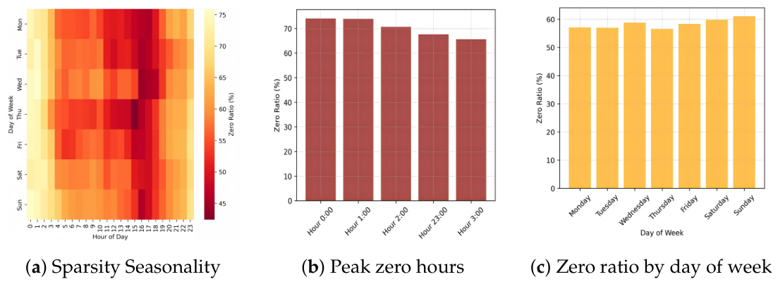
To unravel the temporal structure of sparsity, we analyzed the zero ratio across different time dimensions, which is crucial for identifying predictable periods of low demand or potential station underutilization. Figure 4 illustrates these temporal patterns:

Figure 4. The temporal patterns of zero values.

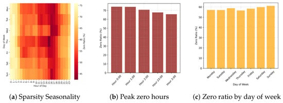
• Hour-of-Day and Day-of-Week Heatmap: The combined influence of daily and weekly cycles on sparsity is comprehensively presented in the heatmap in Figure 4a. This visualization clearly offers valuable insights for optimizing station operations and scheduling maintenance.
• Hourly Zero Ratio: A distinct diurnal pattern is evident in the zero ratio, as depicted in Figure 4b. Early morning periods (0–6 a.m.) consistently demonstrate the highest zero ratios across all days. Sparsity is highest during the early morning hours, peaking at approximately 74.02% around midnight (0:00–1:00 a.m.), and gradually decreasing as the day progresses and charging activity increases. This pattern strongly correlates with typical off-peak hours for vehicle usage.
• Daily Zero Ratio: Figure 4c shows that the zero ratio remains relatively stable throughout the weekdays, hovering between 56% and 58%. However, weekends exhibit a slightly increased zero ratio, reaching 59.80% on Saturday and 61.02% on Sunday. This suggests a general reduction in charging activity during non-working days.

These detailed temporal analyses, encompassing both the occurrence of zero values and actual energy consumption, collectively provide a robust framework for understanding charging station utilization. This addresses the feedback received and offers actionable insights for demand forecasting, network planning, and operational adjustments.

4. Problem Formulation

In a study area comprising a set of n charging stations, each station may accommodate one or more charging sessions. Utilizing the historical data on EV charging demand at the station level, our objective is to develop a predictive model for charging demand across these stations over specified periods (e.g., 6 or 12 h).

Mathematically, let $Y_t$ denote a vector of n elements, where $Y_t^i$ represents the charging load at station i during time period t. Given the historical sequence of EV charging demand over the preceding m time intervals, represented as $[Y_{t-m},Y_{t-m+1},\dots ,Y_{t-1}]$, alongside the corresponding feature set that encapsulates temporal factors and other relevant parameters influencing charging behavior, denoted as $[X_{t-m},X_{t-m+1},\dots ,X_{t-1}]$, our goal is to leverage this information to forecast the charging demand for the next p time intervals, namely:

$$[(Y_{t-m},X_{t-m}),\dots ,(Y_t,X_t)]\stackrel{f(·)}{\to }[Y_{t+1},\dots ,Y_{t+p}]$$

where $0<m<n$ and $0<p<t+p\le n$. This formulation indicates that our deep learning model is designed to learn a function $f(·)$ that effectively predicts future charging demand based on observed historical data.

However, a significant challenge arises from data sparsity within station-level charging demand datasets. As evidenced by the heatmap analysis, many charging stations exhibit limited usage frequency, often resulting in a substantial volume of near-zero observations in the historical data. In some instances, as much as 60% of the recorded sessions for certain stations are zeros, indicating periods devoid of charging events. This phenomenon introduces severe imbalances within the dataset, complicating the task for conventional prediction models to learn effectively, thereby challenging the demand forecasting efforts.

5. Methodology

To effectively address the challenges associated with sparse EV charging load forecasting, we propose a novel forecasting architecture termed the Zero-Inflated Neural Network (ZINN). This architecture is specifically designed to cope with high sparsity datasets while enhancing the accuracy of load predictions.

5.1. Framework Overview

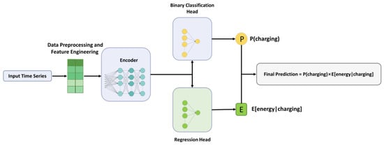
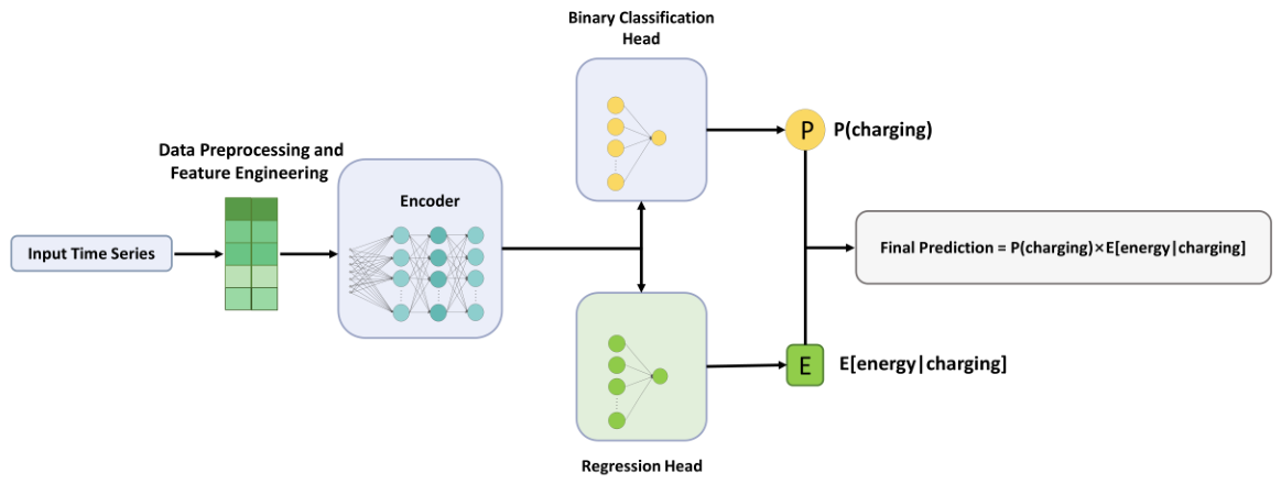
As illustrated in Figure 5, our approach includes three parts:

Figure 5. The overview of EV charging load forecasting. The architecture features a shared feature encoder, a binary head for predicting charging probability, and a regression head for estimating energy consumption.

1.

Encoder: This component learns a compressed representation from input time series of past charging patterns. The input contains: (1) historical energy loads from all stations and (2) features related to each time step.

2.

Binary Head: This component predicts the probability that the charging load is positive at each forecast horizon step for every station. Specifically, for time step $t+\tau$ (within the prediction horizon), the model outputs $p_{t+\tau }=P(y_{t+\tau }>0\mid x_t)\in [0,1]$, which is computed as $p_{t+\tau }=\sigma \left(z_{t+\tau }\right)$ using a sigmoid activation function.

3.

Regression Head: This component estimates the expected energy amount, $E\left[\mathrm{energy}\right|\mathrm{charging}]$, conditional on a charging event taking place. It utilizes a softplus activation function to ensure that predictions remain non-negative.

The final prediction for the charging load at the station is derived from multiplying the outputs of the binary head and the regression head, given by Equation (1):

$$Y_{\mathrm{Final}}=\mathcal{P}\left(\mathrm{charging}\right)\times \mathbb{E}\left[\mathrm{energy}\right|\mathrm{charging}]$$

(1)

5.1.1. Training and Loss Function

The ZINN model is trained using a custom loss function that accounts for both the binary classification of charging events and the regression of energy load predictions. The total loss function is defined as follows:

$${\mathcal{L}}_{\mathrm{total}}={\lambda }_{\mathrm{BCE}}·{\mathcal{L}}_{\mathrm{BCE}}(\mathrm{prob},\mathrm{brinary}\_\mathrm{target})+{\lambda }_{\mathrm{MSE}}·{\mathcal{L}}_{\mathrm{MSE}}(\mathrm{energy},\mathrm{positive}\_\mathrm{targets})$$

(2)

where ${\mathcal{L}}_{\mathrm{BCE}}$ represents the binary cross-entropy loss for the binary head, and ${\mathcal{L}}_{\mathrm{MSE}}$ is the mean squared error for the regression head, evaluated only on non-zero energy values. The coefficients ${\lambda }_{\mathrm{BCE}}$ and ${\lambda }_{\mathrm{MSE}}$ serve as weighting factors to balance the contributions of each component during training.

The effective training of this model is facilitated through techniques such as dropout regularization, early stopping, and adaptive learning rate adjustments, ensuring optimal convergence and generalization performance.

5.1.2. Probabilistic Formulation and Zero-Inflated Likelihood

Let $y_t\ge 0$ denote the charging energy at a given station and time step t. We define a binary charging indicator

$$z_t=\mathbb{I}(y_t>0).$$

The binary head outputs

$${\pi }_t=P(z_t=1\mid x_t)=\sigma \left({\ell }_t\right),$$

where ${\ell }_t$ is the binary head logit and $\sigma (·)$ is the sigmoid function. Conditioned on $z_t=1$, the regression head outputs a non-negative mean

$${\mu }_t=\mathbb{E}[y_t\mid z_t=1,x_t],$$

which is produced by a softplus activation.

We adopt a zero-inflated likelihood that combines a point mass at zero with a continuous distribution for positive values:

$$p(y_t\mid x_t)=(1-{\pi }_t){\delta }_0\left(y_t\right)+{\pi }_t{p}_{+}(y_t;{\mu }_t,{\sigma }^2),$$

where ${\delta }_0(·)$ is a point mass at zero and $p_{+}(y_t;{\mu }_t,{\sigma }^2)$ denotes the density of positive-energy values. In implementation, we model $p_{+}(y_t;{\mu }_t,{\sigma }^2)$ with a Gaussian density on the positive support (treated as an approximation, since ${\mu }_t$ is constrained to be non-negative).

The negative log-likelihood decomposes into a Bernoulli term for zeros and a regression term for non-zeros:

$$\begin{array}{cc}\hfill -logp(y_t\mid x_t)& =-z_{t}log{\pi }_t-(1-z_t)log(1-{\pi }_t)\hfill \\ & +z_t·{\displaystyle \frac{{(y_t-{\mu }_t)}^2}{2{\sigma }^2}}+\mathrm{const}.\hfill \end{array}$$

Therefore, optimizing the binary cross-entropy for the event probability and the mean squared error on positive samples corresponds to maximizing the above zero-inflated likelihood up to additive constants, when ${\sigma }^2$ is treated as fixed. In our total loss in Equation (2), the coefficients ${\lambda }_{\mathrm{BCE}}$ and ${\lambda }_{\mathrm{MSE}}$ re-weight the two decomposed terms to balance classification and regression under high sparsity.

5.1.3. Uncertainty Estimation

To quantify model uncertainty under data sparsity, we use Monte Carlo dropout at inference time. Concretely, we keep dropout active during prediction and draw S stochastic forward passes, obtaining samples ${\{{\pi }_t^{\left(s\right)},{\mu }_t^{\left(s\right)}\}}_{s=1}^S$. The predictive mean energy is approximated by

$$\mathbb{E}\left[y_t\right]\approx {\displaystyle \frac{1}{S}}\sum _{s=1}^S{\pi }_t^{\left(s\right)}{\mu }_t^{\left(s\right)},$$

and the epistemic uncertainty is estimated via the sample variance

$$\mathrm{Var}\left[y_t\right]\approx {\displaystyle \frac{1}{S}}\sum _{s=1}^S{\left({\pi }_t^{\left(s\right)}{\mu }_t^{\left(s\right)}-\mathbb{E}\left[y_t\right]\right)}^2.$$

This uncertainty-aware prediction provides additional information for decision-making in sparse charging regimes.

5.1.4. Handling Sparsity

The unique architecture of ZINN is particularly adept at managing data sparsity for several reasons:

1.

Zero-Inflated Modeling: By employing a binary head for predicting the presence of charging events, the ZINN explicitly models the excess zeros in the dataset. This approach allows the network to differentiate between periods where no charging occurs and periods with actual demand, thus effectively capturing the underlying distribution of the data.

2.

Two-Stage Learning: The separation of the prediction into two stages—determining the probability of a charging event and estimating the energy associated with that event—enables the model to learn relevant features pertinent to both aspects independently. This separation also enhances the model’s ability to identify conditions conducive to actual charging vs. no charging.

3.

Regularization Techniques: ZINN utilizes dropout layers in both heads, which promote model generalization and prevent overfitting to the sparse data, ensuring that the model remains robust even with high-dimensional input features.

4.

Weighted Loss Function: The model employs a custom loss function that balances binary cross-entropy for the probability prediction and mean squared error for the energy prediction, allowing it to focus more on learning from non-zero instances while still penalizing misclassifications effectively.

Through this innovative framework, we aim to provide a robust and reliable solution to the challenges posed by data sparsity in EV charging load forecasting while enhancing model performance and accuracy.

5.2. Evolutionary Structure Search for Zero-Inflated Neural Networks

To avoid manually selecting a single deterministic network structure, we employ an evolutionary architecture search (EA) framework. Given the zero-inflated forecasting objective, the proposed EA automatically discovers effective encoder and head architectures together with key training regularization hyperparameters. This allows the final Zero-Inflated Neural Network to better adapt its inductive bias to sparse (zero-dominated) charging behavior across stations.

5.2.1. Searching Space Definition

We define a comprehensive search space $\mathcal{S}$ that jointly spans (i) the encoder design, (ii) the binary-occurrence head, (iii) the regression (positive-energy) head, and (iv) training hyperparameters:

$$\mathcal{S}=\mathcal{E}\times {\mathcal{H}}_B\times {\mathcal{H}}_R\times \mathcal{R}.$$

(3)

Encoder Space

The encoder search space is defined as

$$\mathcal{E}={\mathcal{T}}_e\times {\mathcal{D}}_h\times {\mathcal{L}}_n\times {\mathcal{D}}_o,$$

(4)

where ${\mathcal{T}}_e\in \{\mathrm{LSTM},\mathrm{GRU},\mathrm{Transformer},\mathrm{iTransformer}\}$ is the encoder type, ${\mathcal{D}}_h\in \{32,64,128,256\}$, is the hidden/model dimension for recurrent encoders, ${\mathcal{L}}_n\in \{1,2,3\}$ is the number of stacked layers, and ${\mathcal{D}}_o\in [0.0,0.3]$ is the dropout rate.

For Transformer-based encoders, we further specify:

$${\mathcal{T}}_{\mathrm{config}}={\mathcal{D}}_m\times {\mathcal{N}}_h\times {\mathcal{D}}_f,$$

(5)

with ${\mathcal{D}}_m\in \{64,128,256\}$ (model dimension), ${\mathcal{N}}_h\in \{2,4,8\}$ (number of attention heads, constrained such that ${\mathcal{D}}_{m}mod{\mathcal{N}}_h=0$), and ${\mathcal{D}}_f\in \{128,256,512\}$ (feed-forward dimension).

Let $t\in {\mathcal{T}}_e$. Given an input sequence $x\in {\mathbb{R}}^{B\times T\times D}$ (batch size B, temporal length T, feature dimension D), the encoder produces:

$${\mathit{h}}_{\mathrm{enc}}={\mathrm{Encoder}}_{\mathit{t}}(\mathit{x}\mathsf{;}{\mathsf{\theta }}_{\mathit{e}})\mathsf{.}$$

(6)

The encoder output dimension $d_{\mathrm{enc}}$ is

$$d_{\mathrm{enc}}=\left\{\begin{array}{cc}{\mathcal{D}}_h,\hfill & \mathrm{if}{\mathcal{T}}_e\in \{\mathrm{LSTM},\mathrm{GRU}\},\hfill \\ {\mathcal{D}}_m,\hfill & \mathrm{if}{\mathcal{T}}_e\in \{\mathrm{Transformer},\mathrm{iTransformer}\}.\hfill \end{array}\right.$$

(7)

Head Space (Binary and Regression)

Both the binary occurrence head and the regression (positive magnitude) head are implemented as MLPs with the following shared structural search form:

$$\mathcal{H}={\mathcal{L}}_{\mathrm{config}}\times {\mathcal{A}}_{\mathrm{act}}\times {\mathcal{D}}_{\mathrm{drop}}\times {\mathcal{B}}_{\mathrm{norm}},$$

(8)

where ${\mathcal{L}}_{\mathrm{config}}$ denotes the choice of hidden-layer widths (e.g., $\left\{\right[64],[128],[64,32],[128,64]$, $[256,128],[128,64,32]\}$), ${\mathcal{A}}_{\mathrm{act}}\in \{\mathrm{ReLU},\mathrm{GELU},\mathrm{ELU},\mathrm{SiLU}\}$ is the activation function, ${\mathcal{D}}_{\mathrm{drop}}\in [0.0,0.3]$ is the dropout rate, and ${\mathcal{B}}_{\mathrm{norm}}\in \{\mathrm{True},\mathrm{False}\}$ indicates whether batch normalization is used.

For prediction horizon (time steps) P and N charging stations, the binary head outputs an occurrence probability:

$$\widehat{\mathit{p}}={\mathrm{Head}}_{\mathit{B}}({\mathit{h}}_{\mathrm{enc}}\mathsf{;}{\mathsf{\theta }}_{\mathit{B}})\in {[\mathbf{0}\mathsf{,}\mathbf{1}]}^{\mathit{B}\times \mathit{P}\times \mathit{N}}\mathsf{,}$$

(9)

and the regression head outputs the non-negative magnitude for positive events:

$${\widehat{\mathit{y}}}_{\mathrm{reg}}={\mathrm{Head}}_{\mathit{R}}({\mathit{h}}_{\mathrm{enc}}\mathsf{;}{\mathsf{\theta }}_{\mathit{R}})\in {\mathbb{R}}_{\ge \mathsf{0}}^{\mathit{B}\times \mathit{P}\times \mathit{N}}\mathsf{.}$$

(10)

Training and Regularization Space

We define the hyperparameter search space as

$$\mathcal{R}={\mathcal{L}}_{\mathrm{rate}}\times {\mathcal{W}}_{\mathrm{decay}}\times {\mathcal{G}}_{\mathrm{clip}}\times {\mathcal{B}}_{\mathrm{momentum}},$$

(11)

where ${\mathcal{L}}_{\mathrm{rate}}\in \{0.0001,0.0005,0.001,0.005\}$ is the learning rate, ${\mathcal{W}}_{\mathrm{decay}}\in \{{10}^{-5},{10}^{-4},{10}^{-3}\}$ is the $L_2$ regularization coefficient, ${\mathcal{G}}_{\mathrm{clip}}\in \{0.5,1.0,1.5,2.0\}$ is the gradient clipping threshold, and ${\mathcal{B}}_{\mathrm{momentum}}\in \{0.01,0.05,0.1,0.9\}$ is the batch-normalization momentum.

Architecture Configuration

A sampled architecture configuration $c\in \mathcal{S}$ is represented as a tuple:

$$\mathit{c}=({\mathit{t}}_{\mathit{e}}\mathsf{,}{\mathit{d}}_{\mathit{h}}\mathsf{,}{\mathit{l}}_{\mathit{n}}\mathsf{,}{\mathit{d}}_{\mathit{o}}^{\mathrm{enc}}\mathsf{,}{\mathit{l}}_{\mathit{B}}\mathsf{,}{\mathit{a}}_{\mathit{B}}\mathsf{,}{\mathit{d}}_{\mathit{B}}\mathsf{,}{\mathit{b}}_{\mathit{B}}\mathsf{,}{\mathit{l}}_{\mathit{R}}\mathsf{,}{\mathit{a}}_{\mathit{R}}\mathsf{,}{\mathit{d}}_{\mathit{R}}\mathsf{,}{\mathit{b}}_{\mathit{R}}\mathsf{,}\mathsf{\alpha }\mathsf{,}\mathit{w}\mathsf{,}\mathit{g}\mathsf{,}\mathit{m})\mathsf{,}$$

(12)

where $\alpha$ denotes the learning rate, w the $L_2$ coefficient, g the gradient clipping threshold, and m the batch-normalization momentum.

5.2.2. Evolutionary Algorithm

We initialize a population ${\mathcal{P}}_0$ by uniformly sampling $\left|P\right|$ configurations:

$${\mathcal{P}}_0=\{c_i^{\left(0\right)}\sim \mathrm{Uniform}\left(\mathcal{S}\right):i=1,\dots ,\left|P\right|\}$$

(13)

Each configuration c is evaluated on the validation set to obtain loss $\mathcal{L}\left(c\right)$. At generation g, we select the top-k parent configurations:

$${\mathcal{P}}_{\mathrm{parent}}^{\left(g\right)}=\mathrm{Top}\text{-}\mathrm{k}({\mathcal{P}}^{(g-1)},k=\lfloor \left|P\right|/2\rfloor )$$

(14)

For each parent $c_p$, mutation modifies attributes with probability $p_m$:

$$c_c\left[a\right]=\left\{\begin{array}{cc}\mathrm{Sample}\left({\mathcal{S}}_a\right)\hfill & \mathrm{with}\mathrm{probability}{p}_m\hfill \\ c_p\left[a\right]\hfill & \mathrm{otherwise}\hfill \end{array}\right.$$

(15)

Key mutable attributes include: encoder type, hidden dimension, layer count, and learning rate. For Transformer configurations, we enforce the constraint ${\mathcal{D}}_{m}mod{\mathcal{N}}_h=0$ to ensure valid attention head configurations.

Crossover combines two parents uniformly:

$$c_c\left[a\right]=\left\{\begin{array}{cc}{c}_{p1}\left[a\right]\hfill & \mathrm{with}\mathrm{probability}0.5\hfill \\ c_{p2}\left[a\right]\hfill & \mathrm{with}\mathrm{probability}0.5\hfill \end{array}\right.$$

(16)

The evolutionary search is formalized in Algorithm 1, terminating after $G_{\max }$ generations. The best configuration $c^{*}$ is returned. Here, $T_{\mathrm{train}}$ denotes the number of training epochs used to train each candidate architecture, and $T_{\mathrm{eval}}$ denotes the number of evaluation epochs/steps used to compute its validation loss.

Algorithm 1 Evolutionary Architecture Search for ZINN.

1:  Initialize population: ${\mathcal{P}}^{\left(0\right)}\sim \mathrm{Uniform}\left(\mathcal{S}\right)$ 2:  for $g=1$ to $G_{\max }$ do 3:      ${\mathcal{P}}_{\mathrm{parent}}^{\left(g\right)}=\mathrm{Top}\text{-}\mathrm{k}({\mathcal{P}}^{(g-1)},k=\lfloor \left|P\right|/2\rfloor )$ 4:      for $i=1$ to $\lfloor \left|P\right|/2\rfloor$ do 5:          if rand() $<p_{\mathrm{crossover}}$ then 6:             $c_c=\mathrm{Crossover}\left(\mathrm{Sample}\text{-}2\left({\mathcal{P}}_{\mathrm{parent}}^{\left(g\right)}\right)\right)$ 7:         else 8:             $c_c=\mathrm{Mutate}\left(\mathrm{Sample}\left({\mathcal{P}}_{\mathrm{parent}}^{\left(g\right)}\right)\right)$ 9:         end if 10:       Train the candidate $c_c$ on ${\mathcal{D}}_{\mathrm{train}}$ for $T_{\mathrm{train}}$ epochs with early stopping (patience: 25 epochs) 11:       Evaluate the trained model on ${\mathcal{D}}_{\mathrm{val}}$ for $T_{\mathrm{eval}}$ steps to obtain $\mathcal{L}\left(c_c\right)$ 12:     end for 13:     ${\mathcal{P}}^{\left(g\right)}=\mathrm{Best}\text{-}\mathrm{k}({\mathcal{P}}_{\mathrm{parent}}\cup {\mathcal{P}}_{\mathrm{offspring}},k=\left|P\right|)$ 14:  end for 15:  Return $c^{*}={arg\; min}_{c\in {\mathcal{P}}^{\left(G_{\max }\right)}}\mathcal{L}\left(c\right)$

Each candidate architecture is first trained on the training set for up to $T_{\mathrm{train}}=50$ epochs with early stopping. The learning rate adjustment scheduler (ReduceLROnPlateau) operates during this training phase, reducing the learning rate when validation loss plateaus (patience: 15 epochs). If the validation loss fails to improve for 25 consecutive epochs, training is halted via early stopping. The evaluation phase then computes the validation loss on a held-out validation set (${\mathcal{D}}_{\mathrm{val}}$) using the best epoch checkpoint, providing the fitness score $\mathcal{L}\left(c\right)$ for architecture ranking.

5.2.3. Architecture Evaluation and Multi-Objective Optimization

Each candidate configuration is evaluated by training on ${\mathcal{D}}_{\mathrm{train}}$ and validating on ${\mathcal{D}}_{\mathrm{val}}$:

$$\mathcal{L}\left(\mathit{c}\right)={\displaystyle \frac{\mathbf{1}}{|{\mathcal{D}}_{\mathrm{val}}|}}\sum _{(\mathit{x}\mathsf{,}\mathit{y})\in {\mathcal{D}}_{\mathrm{val}}}{\parallel \widehat{\mathit{y}}(\mathit{c}\mathsf{,}\mathit{x})-\mathit{y}\parallel }_{\mathbf{2}}^{\mathbf{2}}$$

(17)

To balance accuracy and computational efficiency, we compute a Pareto frontier:

$${\mathcal{P}}_{\mathrm{Pareto}}=\{c\in \mathcal{P}\mid \nexists c^{\prime }\in \mathcal{P}:\mathcal{L}\left(c^{\prime }\right)<\mathcal{L}\left(c\right)\mathrm{and}\theta \left(c^{\prime }\right)<\theta \left(c\right)\}$$

(18)

where $\theta \left(c\right)$ is the total parameter count. The computational complexity of the search is:

$$\mathcal{O}\left(\left(\left|P\right|+G_{\max }·\lfloor \left|P\right|/2\rfloor \right)·(T_{\mathrm{train}}+T_{\mathrm{eval}})\right).$$

(19)

With $G_{\max }=15$, $\left|P\right|=30$, and evaluating approximately $\lfloor \left|P\right|/2\rfloor$ offspring per generation, the total number of candidate trainings is approximately $\left|P\right|+G_{\max }·\lfloor \left|P\right|/2\rfloor =30+15·15=255$. Therefore, the search cost remains practical for deployment scenarios.

6. Experiments

6.1. Experimental Setup

To evaluate the performance of the proposed ZINN architecture, we focus on the task of predicting the charging demand over the next 6 h, utilizing the preceding 24 h of historical data. The choice of 60 min time resolution is justified as follows: (1) Although the average session duration is 2.25 h (Table 1), individual sessions exhibit significant variability (standard deviation 0.60 h), and many sessions are substantially shorter than the mean; (2) a 60 min resolution provides sufficient granularity to capture intra-hour demand variations while remaining computationally efficient; (3) the empirical distribution of session durations shows that approximately 50% of sessions complete within the first 60 min, making this resolution appropriate for capturing rapid charging demand changes; (4) this resolution aligns with standard grid-level demand forecasting and allows for practical operational decision-making at EV charging networks.

A batch size of 64 is employed throughout, and the Adam optimizer is used for training. Moreover, the optimal configuration for the ZINN model structures is automatically discovered by the evolutionary architecture search framework rather than manually configured.

To dynamically adjust the learning rate during training, we utilize the ReduceLROnPlateau scheduler. This method reduces the learning rate by a factor of 0.5 if the validation loss does not show improvement over a specified patience of 15 epochs. It operates in ‘min’ mode, meaning that the scheduler monitors the validation loss, and updates are printed when the learning rate changes, providing transparency into the adjustment process.

An early stopping mechanism is integrated into the training process to prevent unnecessary epochs when the validation loss ceases to improve. This is governed by a patience parameter of 25 epochs, along with a minimum delta of $8\times {10}^{-6}$, which defines the minimum change in loss required for an improvement to be recognized. If the validation loss fails to surpass this threshold over the specified patience period, training is halted.

6.2. Data Preprocessing

6.2.1. Input Data

The input data consists of time series measurements from multiple charging stations with the following characteristics:

• Format: Long-format DataFrame with columns: station_id, period, and energy;
• Time Resolution: Configurable (default: 60 min);
• Handling Missing Values: Zero-filling for missing energy measurements.

6.2.2. Feature Engineering

The following temporal features are automatically generated from the timestamp:

• Hour of day (sine/cosine encoded as shown in Equation (20))

  $$\mathrm{hour}\_\sin =sin\left({\displaystyle \frac{2\pi \times \mathrm{hour}}{24}}\right),\mathrm{hour}\_\cos =cos\left({\displaystyle \frac{2\pi \times \mathrm{hour}}{24}}\right);$$

  (20)
• Day of week (sine/cosine encoded);
• Day of month;
• Month;
• Weekend indicator;
• Business day indicator.

Rationale for sinusoidal encoding: We apply sinusoidal encoding to hour-of-day and day-of-week to capture wrap-around periodicity (e.g., hour 23 and hour 0 are adjacent). Day-of-month and month are encoded as categorical indices rather than sinusoidal functions because they do not exhibit wrap-around structure within our forecasting horizon. This selective encoding strategy improves model interpretability while maintaining computational efficiency.

The feature engineering process produces a total of 47 features, comprising station loads (30 features), and temporal features (17 features). The dataset is split temporally to maintain chronological order, with 70% of the data allocated for training (2184 samples), 15% for validation (468 samples), and 15% for testing (468 samples). This temporal splitting strategy ensures that the model is evaluated on unseen future data, preventing information leakage and providing realistic performance estimates. Each station’s features are normalized independently using Min-Max scaling to map values to the range $[0,1]$, which helps prevent features with larger magnitudes from dominating the learning process while enabling fair comparison across stations with different utilization levels.

6.3. Model Evaluation Metrics

We will use two typical evaluation metrics, namely Mean Absolute Error (MAE) and Root Mean Square Error (RMSE) to evaluate model performance by comparing the difference between the predicted and observed charging demands (denoted as ${\widehat{y}}_t$ and $y_t$, respectively) from different perspectives.

Mean Absolute Error (MAE): The MAE quantifies the error between the predicted and observed EV charging demands. Root Mean Square Error (RMSE): The RMSE index is sensitive to outliers. The RMSE will be relatively large if the difference between the predicted and observed data are large. Therefore, a larger RMSE indicates worse performance of the model.

6.4. ENAS Result Analysis

6.4.1. Search Insights

The evolutionary search process revealed several important architectural patterns:

1.

Attention-Based Superiority: Modern attention mechanisms (iTransformer) outperformed traditional RNN variants, challenging conventional wisdom for time series forecasting.

2.

Asymmetric Head Design: The binary head’s deeper structure ($[128,64,32]$) versus the regression head’s simplicity ($\left[128\right]$) confirms that detecting sparse events requires greater representational capacity than magnitude prediction.

3.

Aggressive Regularization: The dual dropout strategy (0.3 for binary, 0.1 for regression) with batch normalization in the binary head reflects the need for strong regularization when handling high-sparsity data (60.4%).

4.

GELU Activation Dominance: Both heads selected GELU over alternatives (ReLU, ELU, Swish), indicating superior gradient flow and smoother learning dynamics for this task.

5.

Minimal Batch Normalization: The absence of batch normalization in the regression head suggests that per-station feature normalization during preprocessing provides sufficient distributional stability.

This configuration represents a significant advancement over earlier hand-crafted architectures, demonstrating the value of automated architecture discovery in identifying non-obvious yet highly effective designs for specialized forecasting problems.

6.4.2. Best AutoML Configuration

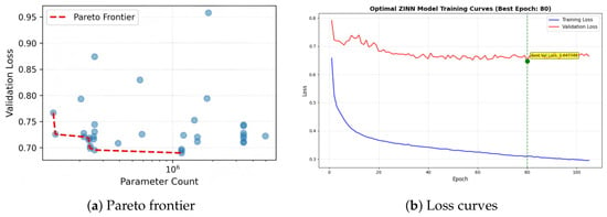
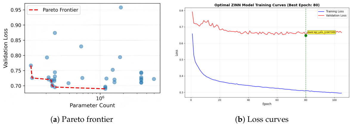
We search for the best configuration based on the lowest validation loss and the lowest parameter count. Figure 6 shows the Pareto frontier of the search space, which represents the set of architectures that achieve both low validation loss and low parameter count.

Figure 6. Evolutionary architecture search analysis: (a) Trade-off between validation loss and model parameter count; (b) Convergence behavior of best configuration showing stable training without overfitting.

The optimal architecture identified by the automated machine learning process exhibits a carefully balanced design across multiple dimensions. Table 2 provides a comprehensive summary of the best configuration discovered by the evolutionary architecture search.

Table 2. Best AutoML configuration for ZINN structure.

Encoder Architecture		Binary Classification Head
Encoder Type	iTransformer	Layer Dimensions	[128, 64, 32]
Model Dimension	256	Activation Function	GELU
Attention Heads	4	Dropout Rate	0.3
Feed-Forward Dimension	512	Batch Normalization	Yes
Number of Layers	1
Encoder Dropout	0.3
Regression Head		Training Configuration
Layer Dimensions	[128]	Learning Rate	0.001
Activation Function	GELU	Weight Decay	$1\times {10}^{-5}$
Dropout Rate	0.1	Gradient Clipping	1.0
Batch Normalization	No	Total Parameters	773,104
		Training Time	≈50.18 s

The selected configuration represents a significant shift toward modern attention-based architectures, favoring the iTransformer encoder over traditional recurrent variants. This choice reflects the evolutionary algorithm’s ability to discover task-specific optimal designs that diverge from conventional choices.

Encoder Architecture: The selection of iTransformer as the encoder demonstrates the effectiveness of inverse-attention mechanisms for time series forecasting. Unlike traditional Transformers that apply attention across time steps, iTransformer treats each time series variable (station) as an independent token, enabling the model to capture inter-variable dependencies more effectively. With a model dimension of 256 and 4 attention heads, the configuration provides sufficient representation capacity while maintaining computational efficiency. The constraint $d_{\mathrm{model}}mod{n}_{\mathrm{heads}}=0$ (i.e., $256mod4=0$) ensures valid attention head configurations. A single layer with 0.3 dropout achieves a balance between learning capacity and regularization, preventing the model from overfitting to the sparse training data.

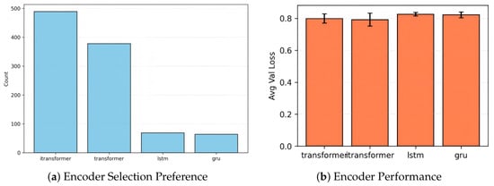
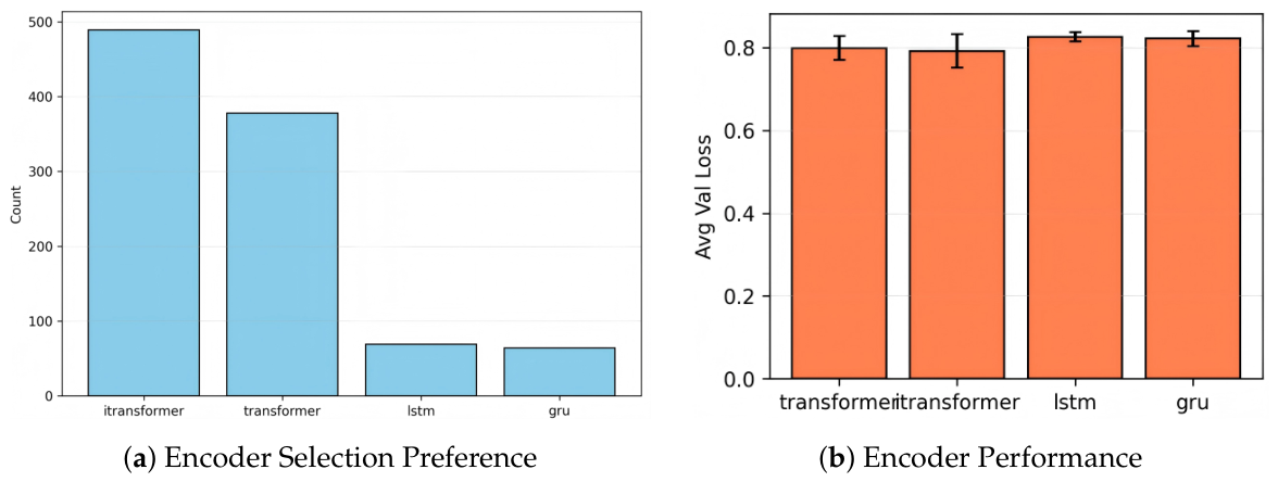
Figure 7 shows the fitness of encoder types regarding selection frequency and average validation loss. The iTransformer encoder is the most frequently selected encoder type, followed by the Transformer encoder. Figure 7b shows the average validation loss of each encoder type. The iTransformer encoder has the lowest average validation loss, indicating its superior performance in this task.

Figure 7. The fitness of encoder types regarding selection freqnecy and average validation loss.

Binary Head Design: The binary classification head employs a deeper structure $[128,64,32]$ compared to the regression head, reflecting the greater complexity of predicting charging occurrence in sparse data. GELU activation functions provide smoother gradients compared to ReLU, facilitating better learning dynamics during backpropagation. The inclusion of batch normalization stabilizes activations across layers, enhancing convergence stability. The aggressive dropout rate of 0.3 provides substantial regularization, critical for preventing overfitting when predicting rare charging events.

Regression Head Design: The regression head employs a simpler single-layer architecture $\left[128\right]$, reflecting that energy magnitude prediction is a more straightforward task once charging occurrence is established. GELU activation ensures smooth non-linear transformations, while the moderate dropout rate of 0.1 provides light regularization appropriate for regression tasks. Notably, batch normalization is absent from this head, suggesting that the binary head’s batch normalization provides sufficient distributional stabilization.

Regularization Strategy: The conservative learning rate of 0.001, combined with minimal weight decay ($1\times {10}^{-5}$) and aggressive gradient clipping (1.0), reflects the need for careful optimization on sparse data. The low weight decay suggests minimal L2 regularization is necessary when dropout and gradient clipping are employed. The small gradient clipping threshold prevents gradient explosion while maintaining directional learning signals.

6.5. Prediction Performance Analysis

The ZINN model was trained for up to 200 epochs, and early stopping was applied at epoch 80 when the validation loss stopped improving. Figure 6b shows the training and validation loss curves. During training, the total loss—comprising the Binary Cross-Entropy (BCE) term for the charging probability and the Mean Squared Error (MSE) term for the positive-energy regression—exhibits stable convergence behavior, indicating effective optimization under high sparsity.

Prediction Visualization and Comparison

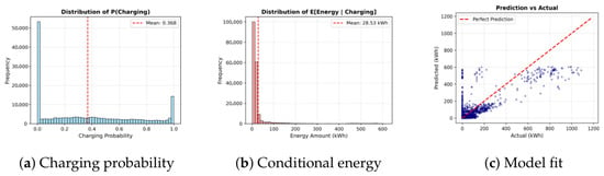
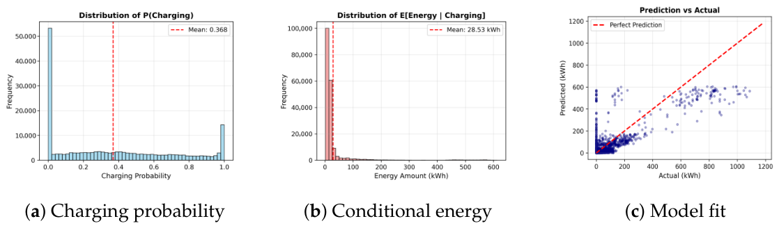
This subsection analyzes the model outputs from both the binary head and the regression head. In Figure 8a, we plot the distribution of the predicted charging probability, denoted by $\mathcal{P}\left(\mathrm{charging}\right)$. Owing to the high sparsity level (approximately 60% zero observations), the model frequently assigns low probabilities to non-charging periods, which is consistent with the empirical charging behavior.

Figure 8. Prediction component analysis: (a) Charging probability distribution; (b) Predicted conditional energy distribution; (c) Actual vs. predicted loads showing overall agreement.

Figure 8b further visualizes the predicted conditional energy, $\mathbb{E}[\mathrm{energy}\mid \mathrm{charging}]$, produced by the regression head. In addition, Figure 8c shows a scatter plot comparing actual vs. predicted loads. Most samples concentrate around the ideal matching line (red), suggesting that the proposed decomposition helps the model capture the overall magnitude of charging demand. Nonetheless, a noticeable deviation appears in the high-energy region, which may be attributed to the interaction between the two heads: the final prediction is modulated by the charging probability, and hence errors in either component can affect the upper tail behavior.

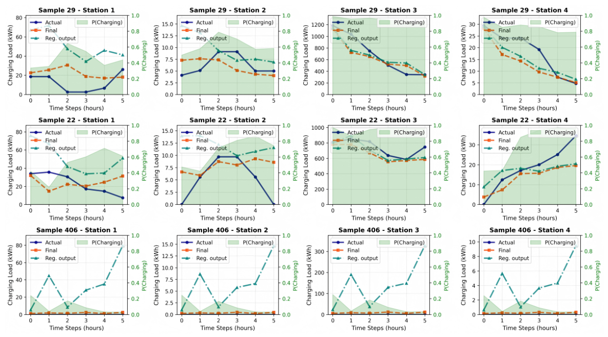
To examine temporal prediction behavior, we selected several representative stations at random and plotted the actual versus predicted charging loads for the next 6 h. Figure 9 compares predictions for 4 different stations. The green shaded region indicates the charging probabilities produced by the binary head, the green dotted line corresponds to the regression head output (predicted conditional energy), and the orange dotted line shows the final load prediction obtained by combining both heads.

Figure 9. ZINN predictions on sample test cases demonstrating the ability to capture diverse charging patterns over a 6 h horizon.

Overall, when charging events occur, the predicted trajectories closely follow the temporal evolution of the ground truth, with discrepancies limited to a small number of time steps. In the subset of samples without charging events (the four cases in the bottom row), the final prediction appropriately remains near zero, consistent with the model successfully identifying non-charging periods from the inferred charging probabilities. These observations suggest that the proposed probability–regression decomposition acts as a critical filter under sparsity: it suppresses spurious positive-energy predictions during inactive periods and yields smoother and more faithful forecasting trends.

6.6. Comparative Performance with Baselines

The proposed ZINN model was evaluated against several baseline forecasting methods, including: (i) GRU and LSTM regressors, (ii) a Transformer regressor, (iii) a Physics-Informed Neural Network (PINN) adapted from [35] for aggregated station-level prediction, (iv) MSTNet, which uses multi-scale temporal convolutional branches, and (v) the strong iTransformer model [23] based on inverse attention for time series forecasting. The overall and non-zero performance are summarized in Table 3, where values in bold are the best performance of ZINN.

Table 3. Comparison of forecasting methods for EV charging load.

Methods	Overall Metrics		Non-Zero Metrics
	MAE	RMSE	MAEnz	RMSEnz	MAPEnz%
GRU Regressor	0.2020	0.2976	0.2456	0.3920	86.89
LSTM Regressor	0.1958	0.2940	0.2524	0.4081	82.12
Transformer Regressor	0.1682	0.2893	0.2900	0.4537	92.40
PINN Regressor	0.1820	0.2934	0.5496	0.6980	78.20
MSTNet Regressor	0.1388	0.2809	0.6386	0.7756	78.66
ZINN (iTransformer)	0.1053	0.2233	0.2206	0.3516	78.18

Across overall metrics, ZINN achieves the best performance with the lowest Overall MAE of 0.1053 and the lowest Overall RMSE of 0.2233. For example, the next best overall performance is achieved by iTransformer with $\mathrm{MAE}=0.1672$ and $\mathrm{RMSE}=0.3575$ (as reported in Table 3).

For non-zero metrics, ZINN remains consistently superior. It attains $MA{E}_{nz}=\mathbf{0}.\mathbf{2206}$ and $RMS{E}_{nz}=\mathbf{0}.\mathbf{3516}$, and it also yields the lowest $MAP{E}_{nz}=\mathbf{78}.\mathbf{18}\%$ among the compared methods. These results indicate that the proposed zero-inflated decomposition is particularly effective in forecasting charging magnitudes when charging events actually take place, rather than only improving performance on the abundant zero portion of the data.

Ablation Study

To validate the effectiveness of the zero-inflated design of ZINN, we conduct controlled ablations. Specifically, after fixing the encoder and head structure, the training pipeline and input data are kept unchanged, while we modify only one component (i.e., we ablate the zero-inflated formulation by using a regression-only variant).

Effect of the zero-inflated component. Table 4 shows that ablation of the zero-inflated design leads to a substantial degradation in zero detection. In particular, while the regression-only variant achieves comparable overall errors (MAE/RMSE differ only marginally: $0.1060/0.2202$ vs. $0.1053/0.2233$), its zero-detection F1-score drops from 79.41% (Full) to 52.50% (Reg-only), indicating that the main limitation comes from incorrect identification of non-charging (zero) states. Interestingly, on non-zero samples, the regression-only variant is competitive in some absolute error metrics; however, the full model achieves a lower non-zero MAPE (78.18 vs. 84.44), suggesting that jointly learning occurrence and magnitude yields more reliable estimates on charging periods.

Table 4. Ablation results for ZINN using iTransformer encoder.

Model	Overall Metrics		Non-Zero Metrics			Zero-Detection Metric
	MAE	RMSE	MAEnz	RMSEnz	MAPEnz%	Acc.%	F1-Score%
Full	0.1053	0.2233	0.2206	0.3516	78.18	84.37	79.41
Reg-only	0.1060	0.2202	0.2151	0.3317	84.44	37.70	52.50

Zero-Detection Performance Metrics. Beyond standard numerical error metrics, ZINN’s binary classification head provides strong discrimination between charging and non-charging states. With a charging probability threshold of 0.5, the full model achieves an accuracy of 84.37%, compared to 37.7% for the regression-only variant. This large gap further confirms that explicitly modeling charging occurrence is essential under sparse and imbalanced conditions.

As reported in Table 4, the full model achieves a zero-detection F1 score of 79.41%, whereas the regression-only baseline reaches only 52.50%. This clear gap highlights that explicitly separating zero (non-charging) from non-zero (charging) states is critical when the forecasting task is dominated by imbalanced observations. Consistent with this design, the distribution of predicted charging probabilities has a mean of 0.38 with noticeable variance, reflecting heterogeneity across stations and time periods.

In comparison to the ablated and regression-only variants, the proposed zero-inflated formulation yields more reliable behavior in sparse charging scenarios. In particular, when compared against additional baselines (e.g., Basic LSTM, Basic Transformer, PINN, and MultiScale Temporal Net), ZINN—and especially the iTransformer-based configuration—maintains superior performance in handling both non-charging intervals and charging events, which is reflected by the consistently stronger zero-detection results.

7. Conclusions

In this study, we developed and evaluated a Zero-Inflated Neural Network for EV charging load forecasting under highly sparse observations. ZINN explicitly models the excess-zero behavior by combining a binary head for charging occurrence with a regression head for non-zero energy estimation. This decomposition enables the model to distinguish charging and non-charging states, alleviating the tendency of purely regression-based objectives to be dominated by abundant zero observations and thereby improving robustness in sparse charging regimes. Overall, ZINN achieves the most accurate forecasting performance among the compared methods, and its zero-detection capability demonstrates clear gains over a regression-only variant. From a methodological perspective, the binary–regression decomposition offers a principled mechanism for suppressing spurious positive predictions during non-charging periods while improving the fidelity of energy estimates when charging events occur. These results indicate that ZINN provides an effective and practical framework for station-level forecasting, supporting more reliable energy management and operational planning for EV charging infrastructures.

Limitations and Future Work. First, our discretization assumes that the energy variable $y_t$ represents the (near) total charging energy within each fixed time bin (default 60 min); consequently, the derived zero/non-zero indicator $z_t=\mathbb{I}(y_t>0)$ is conditional on this aggregation. Second, station identity is inferred from GPS-based DBSCAN clustering of session start coordinates, assuming that GPS noise and short-term mobility do not materially change station assignment. Additionally, while the proposed zero-inflated likelihood is formulated in a probabilistic manner, the positive-energy density is implemented as a Gaussian approximation with a fixed variance term, which may limit calibration for heavy-tailed magnitude distributions. Our experiments are conducted on a single city and do not include direct auxiliary operational variables (e.g., station downtime, maintenance schedules), which could affect zero patterns. We therefore treat the reported improvements as evidence of benefit under comparable data conditions and recommend further validation on multi-city datasets with richer metadata. We did not compare against classical zero-inflated or hurdle statistical models; future work will incorporate such baselines to quantify the incremental benefit of the neural decomposition and further improve interpretability across sparse forecasting settings.

References

- Alšauskas, O.; Connelly, E.; Huismans, M.; Jenness, E.; Copier, J.J.; Marois, J.L.; Lombardo, T.; McDonagh, S.; O’Riordan, V.; Petropoulos, A.; et al. Global EV Outlook 2024; Technical Report; International Energy Agency: Paris, France, 2024. [Google Scholar]
- Yang, Y.; Zhu, B.; She, X.; Wang, K.; Liu, A. A Family of Bipolar DC–DC Converters With Interpolar Voltage Self-Balancing Based on FB-BVMs for BLVDC Microgrid. IEEE Trans. Ind. Electron. 2025, 72, 9229–9238. [Google Scholar] [CrossRef] [Scilit]
- He, C.; Zhu, J.; Lan, J.; Li, S.; Wu, W.; Zhu, H. Optimal planning of electric vehicle battery centralized charging station based on EV load forecasting. IEEE Trans. Ind. Appl. 2022, 58, 6557–6575. [Google Scholar] [CrossRef] [Scilit]
- Li, H.; Zhu, J.; Zhou, Y.; Feng, D.; Zhang, K.; Shen, B. Review of load forecasting methods for electric vehicle charging station. In Proceedings of the 2022 IEEE/IAS Industrial and Commercial Power System Asia (I&CPS Asia); IEEE: Piscataway, NJ, USA, 2022; pp. 1833–1837. [Google Scholar]
- Hochreiter, S.; Schmidhuber, J. Long short-term memory. Neural Comput. 1997, 9, 1735–1780. [Google Scholar] [CrossRef] [Scilit] [PubMed]
- Vaswani, A.; Shazeer, N.; Parmar, N.; Uszkoreit, J.; Jones, L.; Gomez, A.N.; Kaiser, L.; Polosukhin, I. Attention is all you need. In Proceedings of the 31st International Conference on Neural Information Processing Systems (NIPS’17), Long Beach, CA, USA, 4–9 December 2017; pp. 6000–6010. [Google Scholar]
- You, L.; Zhu, R.; Kwan, M.P.; Chen, M.; Zhang, F.; Yang, B.; Wong, M.S.; Qin, Z. Unraveling adaptive changes in electric vehicle charging behavior toward the postpandemic era by federated meta-learning. Innovation 2024, 5, 100587. [Google Scholar] [CrossRef] [Scilit] [PubMed]
- Yang, Y.; Zhu, B.; She, X.; Wang, K.; Liu, A. A Family of Voltage Balancers With Fault-Tolerance and Interpolar Voltage Self-Balancing Ability for Bipolar DC Power Systems. IEEE Trans. Transp. Electrif. 2025, 11, 9864–9876. [Google Scholar] [CrossRef] [Scilit]
- Arias, M.B.; Bae, S. Electric vehicle charging demand forecasting model based on big data technologies. Appl. Energy 2016, 183, 327–339. [Google Scholar] [CrossRef] [Scilit]
- Wu, D.; Zhang, F.; Lou, W.; Li, D.; Chen, J. Chemical characterization and toxicity assessment of fine particulate matters emitted from the combustion of petrol and diesel fuels. Sci. Total Environ. 2017, 605–606, 172–179. [Google Scholar] [CrossRef] [Scilit]
- Jeon, Y.E.; Kang, S.B.; Seo, J.I. Hybrid Predictive Modeling for Charging Demand Prediction of Electric Vehicles. Sustainability 2022, 14, 5426. [Google Scholar] [CrossRef] [Scilit]
- Pasha, J.; Li, B.; Elmi, Z.; Fathollahi-Fard, A.M.; yip Lau, Y.; Roshani, A.; Kawasaki, T.; Dulebenets, M.A. Electric vehicle scheduling: State of the art, critical challenges, and future research opportunities. J. Ind. Inf. Integr. 2024, 38, 100561. [Google Scholar] [CrossRef] [Scilit]
- Zhou, N.; Xiong, X.; Wang, Q. Probability Model and Simulation Method of Electric Vehicle Charging Load on Distribution Network. Electr. Power Components Syst. 2014, 42, 879–888. [Google Scholar] [CrossRef] [Scilit]
- Huang, X.; Wu, D.; Boulet, B. Ensemble learning for charging load forecasting of electric vehicle charging stations. In Proceedings of the 2020 IEEE Electric Power and Energy Conference (EPEC); IEEE: Piscataway, NJ, USA, 2020; pp. 1–5. [Google Scholar]
- Majidpour, M.; Qiu, C.; Chu, P.; Pota, H.R.; Gadh, R. Forecasting the EV charging load based on customer profile or station measurement? Appl. Energy 2016, 163, 134–141. [Google Scholar] [CrossRef] [Scilit]
- Lu, Y.; Li, Y.; Xie, D.; Wei, E.; Bao, X.; Chen, H.; Zhong, X. The Application of Improved Random Forest Algorithm on the Prediction of Electric Vehicle Charging Load. Energies 2018, 11, 3207. [Google Scholar] [CrossRef] [Scilit]
- Cho, K.; van Merriënboer, B.; Gulcehre, C.; Bahdanau, D.; Bougares, F.; Schwenk, H.; Bengio, Y. Learning Phrase Representations using RNN Encoder–Decoder for Statistical Machine Translation. In Proceedings of the 2014 Conference on Empirical Methods in Natural Language Processing (EMNLP); Moschitti, A., Pang, B., Daelemans, W., Eds.; Association for Computational Linguistics: Doha, Qatar, 2014; pp. 1724–1734. [Google Scholar] [CrossRef] [Scilit]
- Zhu, J.; Yang, Z.; Guo, Y.; Zhang, J.; Yang, H. Short-term load forecasting for electric vehicle charging stations based on deep learning approaches. Appl. Sci. 2019, 9, 1723. [Google Scholar] [CrossRef] [Scilit]
- Zhu, J.; Yang, Z.; Mourshed, M.; Guo, Y.; Zhou, Y.; Chang, Y.; Wei, Y.; Feng, S. Electric vehicle charging load forecasting: A comparative study of deep learning approaches. Energies 2019, 12, 2692. [Google Scholar] [CrossRef] [Scilit]
- Zhang, X.; Chan, K.W.; Li, H.; Wang, H.; Qiu, J.; Wang, G. Deep-learning-based probabilistic forecasting of electric vehicle charging load with a novel queuing model. IEEE Trans. Cybern. 2020, 51, 3157–3170. [Google Scholar] [CrossRef] [Scilit]
- Mohammad, F.; Kang, D.K.; Ahmed, M.A.; Kim, Y.C. Energy demand load forecasting for electric vehicle charging stations network based on convlstm and biconvlstm architectures. IEEE Access 2023, 11, 67350–67369. [Google Scholar] [CrossRef] [Scilit]
- Li, Y.; Yang, C.; Zeng, H.; Dong, Z.; An, Z.; Xu, Y.; Tian, Y.; Wu, H. Frequency-aligned knowledge distillation for lightweight spatiotemporal forecasting. In Proceedings of the IEEE/CVF International Conference on Computer Vision; IEEE: Piscataway, NJ, USA, 2025; pp. 7262–7272. [Google Scholar]
- Liu, Y.; Hu, T.; Zhang, H.; Wu, H.; Wang, S.; Ma, L.; Long, M. iTransformer: Inverted Transformers Are Effective for Time Series Forecasting. In Proceedings of the International Conference on Learning Representations; Kim, B., Yue, Y., Chaudhuri, S., Fragkiadaki, K., Khan, M., Sun, Y., Eds.; International Conference on Learning Representations (ICLR): Appleton, WI, USA, 2024; Volume 2024, pp. 11116–11140. [Google Scholar]
- Hussain, A.; Eswarakrishnan, V.; Aslam, A.; Tripura, S. Charging stations demand forecasting using LSTM based hybrid transformer model. Sci. Rep. 2025, 15, 36639. [Google Scholar] [CrossRef] [Scilit]
- Lambert, D. Zero-inflated Poisson regression, with an application to defects in manufacturing. Technometrics 1992, 34, 1–14. [Google Scholar] [CrossRef] [Scilit]
- Mullahy, J. Specification and testing of some modified count data models. J. Econom. 1986, 33, 341–365. [Google Scholar] [CrossRef] [Scilit]
- Yang, H. Bayesian Zero-Inflated Model for Ordinal Data. Master’s Thesis, University of South Carolina, Columbia, SC, USA, 2020. [Google Scholar]
- Neelon, B.; O’Malley, A.J.; Smith, V.A. Modeling zero-modified count and semicontinuous data in health services research Part 1: Background and overview. Stat. Med. 2016, 35, 5070–5093. [Google Scholar] [CrossRef] [Scilit]
- Zoph, B.; Vasudevan, V.; Shlens, J.; Zou, Q.V. Neural architecture search with reinforcement learning. In Proceedings of the International Conference on Learning Representations (ICLR), Toulon, France, 24–26 April 2017. [Google Scholar]
- Real, E.; Aggarwal, A.; Huang, Y.; Le, Q.V. Regularized evolution for image classifier architecture search. Proc. AAAI Conf. Artif. Intell. 2019, 33, 4780–4789. [Google Scholar] [CrossRef] [Scilit]
- Klein, A.; Falkner, S.; Springenberg, J.; Hutter, F. Fast Bayesian optimization of machine learning hyperparameters on large datasets. In Proceedings of the Artificial Intelligence and Statistics; PMLR: Cambridge, MA, USA, 2019; pp. 528–536. [Google Scholar]
- Liu, H.; Simonyan, K.; Yang, Y. DARTS: Differentiable architecture search. In Proceedings of the International Conference on Learning Representations (ICLR), New Orleans, LA, USA, 6–9 May 2019. [Google Scholar]
- Sun, Y.; Xue, B.; Zhang, M. Evolving deep convolutional neural networks for image classification. IEEE Trans. Evol. Comput. 2020, 24, 394–407. [Google Scholar] [CrossRef] [Scilit]
- Elsken, T.; Metzen, J.H.; Hutter, F. Neural architecture search: A survey. J. Mach. Learn. Res. 2019, 20, 1997–2017. [Google Scholar]
- Kuang, H.; Qu, H.; Deng, K.; Li, J. A physics-informed graph learning approach for citywide electric vehicle charging demand prediction and pricing. Appl. Energy 2024, 363, 123059. [Google Scholar] [CrossRef] [Scilit]
Disclaimer/Publisher’s Note: The statements, opinions and data contained in all publications are solely those of the individual author(s) and contributor(s) and not of MDPI and/or the editor(s). MDPI and/or the editor(s) disclaim responsibility for any injury to people or property resulting from any ideas, methods, instructions or products referred to in the content. |
© 2026 by the authors. Licensee MDPI, Basel, Switzerland. This article is an open access article distributed under the terms and conditions of the Creative Commons Attribution (CC BY) license.