


Abstract
Large-scale and widely distributed air-conditioning (AC) loads can be aggregated into load-type Virtual Power Plants (VPPs) to participate in peak-shaving ancillary services, thereby improving the allocation of demand-side electricity resources. However, current AC aggregation methods primarily focus on meeting peak-shaving instructions and generally employ fixed incentive pricing and proportional capacity allocation, making it difficult to balance user revenue and satisfaction and thereby constraining the flexibility of VPP demand-side regulation. This paper proposes a unified incentive-based demand response scheduling framework for both fixed- and variable-frequency AC loads across industrial, commercial, and residential scenarios. Based on the Equivalent Thermal Parameter model, AC loads are classified into curtailable and shiftable types, with their adjustable boundaries characterized by a Time-of-Use (TOU) elasticity-based interaction willingness model and a fuzzy load transfer rate model, respectively. A three-objective optimization model is established to maximize user revenue while minimizing user dissatisfaction and scheduling error, with incentive pricing and capacity allocation jointly optimized via Non-dominated Sorting Genetic Algorithm III (NSGA-III). Case studies are conducted on a load-type VPP covering three scenarios, namely a large industrial zone, a commercial zone, and a residential zone, under weekday and non-weekday TOU tariffs and three representative 1 h peak-shaving periods. Compared with a fixed-pricing benchmark, the proposed strategy increases total user revenue by 9.4% to 11.4% and reduces weighted average dissatisfaction by 0.27 to 1.92%. The case study results demonstrate that the proposed method can improve the trade-off between user revenue and satisfaction.
1. Introduction
The large-scale integration of renewable energy, coupled with the ongoing development of electricity spot and ancillary service markets, has increased the need for flexible regulating resources in power systems. In this context, VPPs, which aggregate distributed energy resources, energy storage systems, and flexible loads, have become an important means of linking user-side flexibility with grid-side regulation needs [1,2,3]. Previous studies have shown that heating, ventilation, and AC systems can provide peak-shaving and load-shifting capability at the building-cluster level through setpoint adjustment, pre-cooling/pre-heating, and power limiting [4,5]. Among these resources, AC loads are regarded as one of the most promising flexible resources for demand response because of their strong thermal inertia, fast response, large installed capacity, and adjustable comfort settings. Nevertheless, constraints related to thermal comfort, heterogeneity in participation willingness, and differences in perceived economic benefits continue to hinder the sustained and reliable participation of AC resources in grid-interactive regulation [6].
Existing studies on AC load scheduling can generally be divided into two streams. One stream focuses on load aggregation and control. Relevant research has explored the quantification of HVAC flexibility, building demand flexibility, and various AC control strategies [7,8,9]. Established methodologies have been developed for demand response control, multi-agent coordinated regulation, and adaptive decentralized control of large-scale variable-frequency AC clusters [10,11,12]. Some studies have further addressed variable-frequency and residential AC scheduling from an engineering application perspective [13,14]. Additionally, some research has examined the distinct characteristics of fixed-frequency and variable-frequency ACs across multiple scenarios, as well as the influence of user willingness to interact on adjustable potential [15]. Recent studies have further shown that differentiated economic benefit and thermal comfort requirements of AC users should be explicitly considered when designing demand response strategies [16]. Overall, this line of research has achieved substantial progress in aggregation modeling, response boundary analysis, and tracking control. However, it primarily focuses on improving execution efficiency and tracking accuracy, with insufficient attention given to the coordinated optimization of user incentives and scheduling decisions.
The other stream focuses on market-oriented VPP operation and scheduling. In this line of research, dynamic incentive pricing, user satisfaction, comfort loss, and market revenue have been gradually integrated into unified scheduling frameworks. Existing studies have examined VPP bidding under dynamic demand response prices and integrated satisfaction constraints [17], as well as urban VPP operation under incentive-based demand response and two-stage robust optimization with refined demand response [18,19]. More recent studies have also investigated incentive-based demand response and hierarchical VPP operation while accounting for user participation uncertainty and aggregator-side satisfaction [20,21]. Related VPP research has further expanded to multi-market participation and demand-side ancillary-service operation [22,23]. However, most studies focus on generic flexible loads or integrated VPP portfolios, neglecting the heterogeneous response characteristics of fixed-frequency and variable-frequency AC loads across industrial, commercial, and residential scenarios. In addition, relatively few studies have jointly optimized capacity allocation and incentive pricing. In load-type VPPs, the demand response capability of AC loads is highly scenario-dependent, because it is jointly constrained by thermal comfort, building thermal inertia, response duration, and user participation heterogeneity across fixed-frequency/variable-frequency units and industrial, commercial, and residential settings.
In practical operation, the participation of a load-type VPP in ancillary services involves two layers: external market bidding, clearing, and settlement, as well as internal resource organization and incentive scheduling following a peak-shaving request. Existing studies have not effectively combined multi-scenario aggregation modeling of fixed- and variable-frequency AC loads with differentiated incentive design, nor have they unified curtailable and shiftable load characteristics within a joint optimization framework for capacity allocation and incentive pricing. Therefore, unlike studies that focus primarily on AC control performance or on VPP market bidding with generic flexible loads, this paper addresses the internal coordination problem of a load-type VPP after receiving a peak-shaving command, with emphasis on jointly evaluating scenario-dependent AC response capability and enabling differentiated incentive-based capacity allocation. Specifically, fixed- and variable-frequency AC loads across industrial, commercial, and residential scenarios are modeled within a unified framework that combines load aggregation, response-boundary characterization, and the coordinated optimization of incentive pricing and capacity allocation. In this manner, the study contributes not only to demand response scheduling for power system flexibility, but also to understanding how user willingness and satisfaction affect the practical adoption of flexible load resources in smart grid-oriented VPP operation.
The main contributions of this paper are as follows:
- A unified aggregation and response-boundary modeling framework has been established for fixed-frequency and variable-frequency AC loads in industrial, commercial, and residential scenarios. By distinguishing between curtailable loads and shiftable loads, we characterize the actual adjustable boundaries of the two load types using a TOU elasticity-based user interaction willingness model and a triangular membership function-based load transfer rate model, respectively.
- Under a given upper-level peak-shaving requirement, a three-objective coordinated scheduling model is developed for multi-scenario AC resources within a load-type VPP. Unlike studies focused mainly on control performance or external market bidding, the model jointly optimizes capacity allocation and incentive pricing while balancing user revenue, user satisfaction, and scheduling accuracy.
- Comparative case studies against a benchmark with fixed pricing and proportional allocation show that differentiated incentive pricing can reallocate AC response capacity across scenarios, thereby improving the trade-off among economic performance, user satisfaction, and scheduling effectiveness.
2. Air Conditioning Load Modeling
The Equivalent Thermal Parameter (ETP) model describes the thermodynamic characteristics of an AC system under different operating conditions through the energy balance Equation and thermodynamic cycle. The first-order ETP model is governed by the following equation:
where is the indoor temperature; is the outdoor temperature (°C); is the cooling capacity of the AC (kW); R is the equivalent thermal resistance of the AC–building system (°C/kW); and C is the equivalent thermal capacitance of the AC–building system (kJ/°C).
2.1. Fixed-Frequency AC Aggregation Model
A fixed-frequency AC unit operates cyclically, with its on/off state determined by comparing the indoor temperature to the setpoint temperature. The cooling capacity, denoted as , is expressed as
where the subscript ff denotes the fixed-frequency AC; superscript u and d represent the upper and lower limits, respectively; is the electrical power at time t; is the rated power; η is the coefficient of performance (COP); is the on/off state variable (0 = off, 1 = on); is the setpoint temperature; is the sampling time step; and are the upper and lower deadband limits, respectively; and is the deadband width.
Assuming that the outdoor temperature remains constant, can be expressed as
where is the constant in the general solution of the differential equation.
When the AC system is activated (i.e., ), setting the indoor temperature equal to the upper deadband limit and the lower deadband limit , respectively, yields the off-duration and the on-duration within a single operating cycle
where and .
For load aggregators and dispatch centers, the aggregated power of a large-scale AC fleet is of primary interest. Since the aggregated power of fixed-frequency ACs depends solely on the number of units currently operating, the duty cycle is introduced to represent the probability that a single unit is on at time t. The average electrical power of one fixed-frequency AC unit over its operating cycle is
where i is the unit index, is the rated power of unit i, is the cycle’s average power, and is the duty cycle of unit i.
Since the on-to-off time ratio of a fixed-frequency AC in a single cycle is typically around 1:2, the condition is satisfied. Equation (8) can therefore be transformed into the following inequality:
Assuming that the number of operating units N is sufficiently large and that each unit runs independently, the aggregated power of N fixed-frequency AC units at time t under constant outdoor temperature is
where the subscript agg denotes aggregation.
Incorporating the expectation operator into inequality (9), the upper and lower bounds of the aggregated power, and , are obtained as
where E(·) denotes the mathematical expectation.
The aggregated baseline power of the fixed-frequency AC load can then be expressed as
where is the allocation coefficient.
It follows from Equation (13) that the aggregated power of the fixed-frequency AC load is determined by the number of operating units N, the outdoor temperature , the expected setpoint temperature , the expected deadband width , the allocation coefficient , the expected COP , and the expected equivalent thermal resistance . Equation (13) is derived under the assumptions of approximately constant within each scheduling interval and statistically independent operation of a large AC population, which are appropriate for the hour-level scheduling considered here.
2.2. Variable-Frequency AC Aggregation Model
Unlike fixed-frequency ACs, the compressor speed of a variable-frequency AC varies between its maximum and minimum operating frequencies in response to changes in indoor temperature relative to the setpoint. For instance, in cooling mode, the relationship between compressor frequency and indoor temperature can be described as follows:
where is the compressor frequency at indoor temperature ; the subscript vf denotes the variable-frequency AC; and are the upper and lower frequency limits; and are the lower and upper deadband limits; and is the cut-off temperature, generally set to . When the indoor temperature falls below , the compressor stops and the unit enters standby mode.
The cooling capacity and the electrical power of a variable-frequency AC are both expressed as linear functions of the compressor frequency f:
The default regulation method for variable-frequency AC aggregation involves adjusting the temperature setpoint. When the setpoint is altered at a specific moment, both the operating power and the indoor temperature respond accordingly. After a brief transition period, the AC system reaches a new steady state. Assuming that this transition is sufficiently brief, only the steady-state changes should be considered in the aggregation model, thereby allowing for the neglect of transient dynamics.
Assuming a constant outdoor temperature during the regulation period and that the indoor temperature stabilizes at the setpoint, substituting these conditions into Equation (1) yields the steady-state cooling capacity :
where is the setpoint temperature of the variable-frequency AC.
Substituting Equation (17) into Equations (15) and (16), the steady-state power is obtained as
Introducing the expectation operator and aggregating N variable-frequency AC units, the aggregated power is
From the analysis of Equation (19), it can be concluded that the aggregated power of variable-frequency AC loads can be determined by several variables: the number of operating units N, the outdoor temperature , the expected setpoint temperature , the expected fitting coefficients , and the expected equivalent thermal resistance . Equation (19) further assumes that transient responses after setpoint changes are negligible over the scheduling interval, which is appropriate for the hour-level scheduling considered here but may reduce accuracy for shorter intervals or pronounced thermal lag.
2.3. Curtailable Load Modeling
Building on the aggregation models developed in Section 2.1 and Section 2.2, two typical types of AC scheduling response can be analyzed. Curtailable loads are defined as AC loads whose operating power is reduced by increasing the temperature setpoint within a specified time window. Typical scenarios include residential- and commercial-building AC systems, where both the curtailment capacity and duration are limited by user comfort requirements. According to Equation (19), the difference between the aggregated power before and after the setpoint adjustment represents the objectively available regulation potential. The adjusted aggregated load satisfies
where is the adjusted aggregated power of the curtailable load in period t; is the pre-adjustment aggregated power; is the aggregated curtailment in period t; is the total curtailment over the regulation period T; and is the upper bound on curtailment in period t.
2.3.1. User Interaction Willingness Quantification Model
Calculating the adjustable potential of AC loads necessitates careful consideration of both objective and subjective factors. The objective factor refers to the inherent regulatory potential of the AC load itself, while the subjective factor pertains to the user’s willingness to engage in regulation. As electricity markets continue to evolve, user willingness to interact is primarily influenced by their sensitivity to TOU pricing. When the actual electricity price does not exceed the user’s expected price, their willingness to participate is either zero or negative, resulting in no incentive for engagement. Conversely, when the actual price surpasses the expected price, users are inclined to participate in order to mitigate electricity costs; notably, the greater the price differential, the stronger the willingness to engage. Additionally, an amplification coefficient α is introduced to account for non-price factors such as the type of day and operational conditions.
Users participating in regulation are classified by scenario, distinguishing between industrial/commercial and residential settings, as well as by day type, categorizing days into weekdays and non-weekdays. The willingness of users to engage in regulation in scenario j under day type k is defined as follows:
where is the scenario index and is the day-type index; ; is the expected electricity price; is the current actual price; is the peak-period price; and is the amplification coefficient capturing the influence of non-price factors.
The AC regulation lowers the compressor frequency by raising the temperature setpoint, thereby reducing the total power consumption. The willingness of users to interact with the system determines the acceptable magnitude of setpoint increase. Based on this willingness , the elastic range for temperature adjustment is determined as follows:
where and are the original upper and lower deadband limits before regulation; and are the updated deadband limits after regulation.
2.3.2. Curtailable Load Scheduling Response Model
Based on the AC aggregation models presented in Section 2.1 and Section 2.2, when user interaction willingness is not considered, the potential for objective regulation of the curtailable load is equivalent to the difference in the aggregated power before and after the adjustment of the setpoint
where and are the objective regulation potentials of the fixed- and variable-frequency AC aggregations, respectively, without considering interaction willingness; and are the aggregated powers of the fixed-frequency fleet before and after setpoint adjustment; and are the corresponding values for the variable-frequency fleet; and are the setpoint adjustment magnitudes for the respective fleets.
Incorporating both objective and subjective factors, the total AC load curtailment for n scenarios under day type k at time t is
2.4. Shiftable Load Modeling
Unlike curtailable loads, shiftable loads respond to scheduling commands by shifting their electricity consumption over time rather than reducing the total amount consumed. Typical examples include industrial production equipment and time-flexible AC loads in commercial buildings. The response of shiftable AC loads results in a shift in the load curve along the time dimension, making it impossible to directly infer the actual response magnitude from the original forecasted load. Consequently, this paper introduces a load transfer rate, defined as the ratio of load shifted from high-price periods to low-price periods relative to the original load during the high-price period. This metric effectively characterizes users’ temporal shifting behavior under TOU pricing incentives. Based on Equation (19), the adjusted aggregated power of shiftable ACs is satisfied:
where is the adjusted aggregated power of the shiftable load in period t; is the pre-adjustment aggregated power; is the aggregated shift amount in period t (positive for inflow, negative for outflow); and and are the upper and lower bounds of the shift amount in period t.
2.4.1. Load Transfer Rate Model
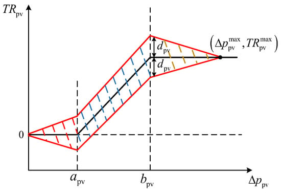
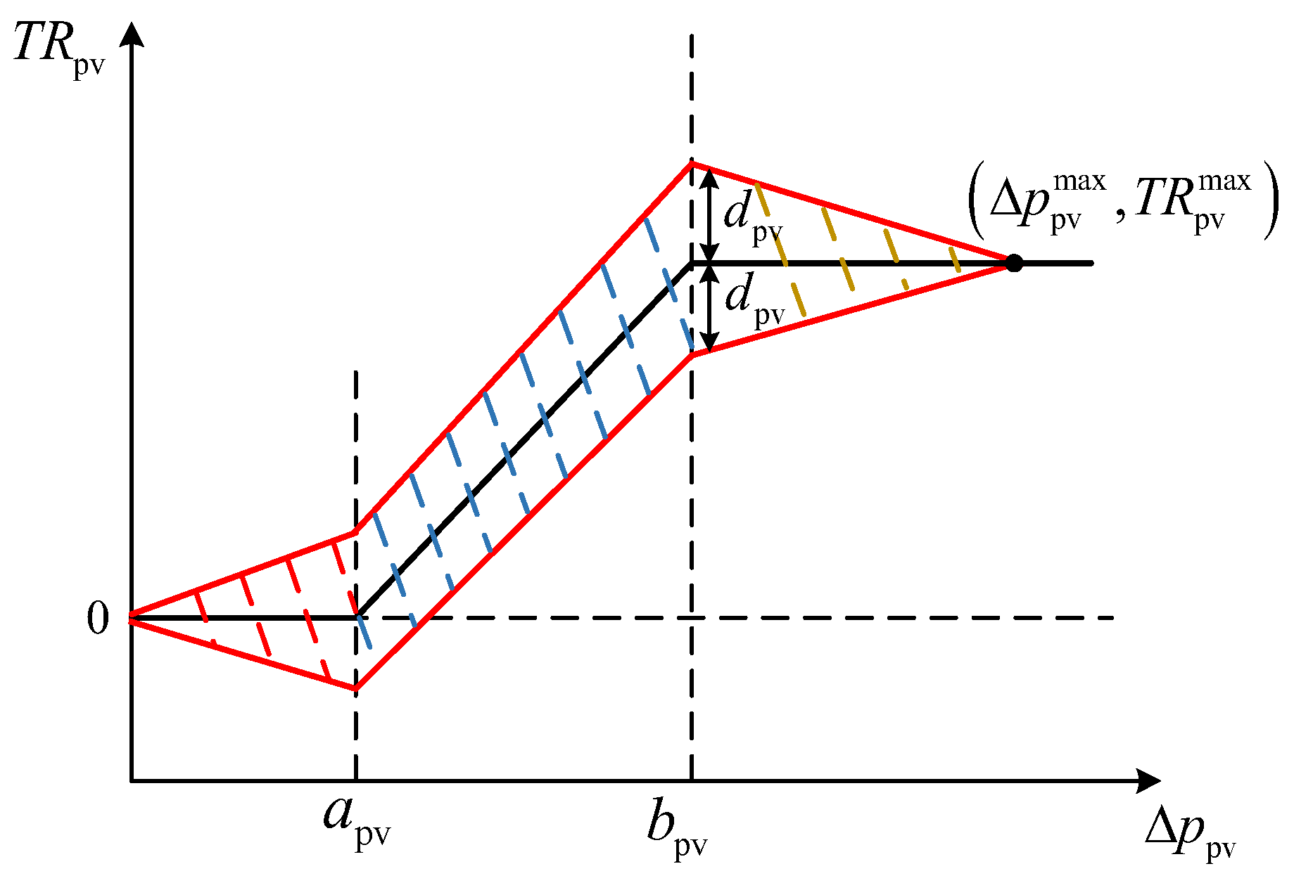
Under TOU pricing, a fuzzy approach utilizing triangular membership functions is employed to characterize the response rate of shiftable AC loads. The response of the load to price incentives is categorized into three distinct zones: a dead zone, a linear zone, and a saturation zone. The load transfer rate is defined as the ratio of the load shifted from peak-price periods to valley-price periods, relative to the original load during the peak period, as illustrated in Figure 1.
Figure 1.
Load transfer rate curve accounting for user response heterogeneity.
In Figure 1, the solid black curve illustrates the load transfer rate based on principles of consumer psychology, while the area enclosed by the solid red lines delineates the maximum fluctuation range of the transfer rate. Within both the dead zone and linear zone, the price incentive is insufficient to alter electricity consumption behavior; the prevailing uncertainty is primarily attributed to non-economic factors, such as established consumption habits. As the incentive intensifies and the response rate escalates, external factors, including weather conditions, become increasingly significant, thereby amplifying uncertainty. In the saturation zone, economic factors dominate, leading to a stabilization of response behavior, with uncertainty diminishing towards zero.
As shown in Figure 1, the load transfer rate varies with the peak-to-valley price differential . When , the response remains near zero (dead zone). When , increases with the price differential (linear zone). When , the response approaches its upper limit (saturation zone). The red envelope denotes the uncertainty range . Accordingly, Equation (31) describes the piecewise transfer-rate curve, and Equation (32) gives the variation in the uncertainty width .
Based on Figure 1, fuzzy numbers are utilized to represent the actual load response rate, while triangular membership functions characterize the degree of variation in this response rate. The peak-to-valley transfer rate under TOU pricing is expressed as follows:
where is the actual peak-to-valley load transfer rate; is the rate-of-change coefficient of the transfer rate with respect to the peak-to-valley price differential in the linear zone; is the actual peak-to-valley price differential; is the maximum value of the price differential; and are the price differentials at the dead-zone and saturation-zone inflection points, respectively; is the upper limit of ; and is the maximum fluctuation range of the peak-to-valley transfer rate.
The maximum fluctuation range serves as a parameter of the membership function; . After exceeds , the price differential becomes the dominant factor governing the fluctuation of the transfer rate, and decreases toward zero. Its expression is
where and are the coefficients for the rate of change of before and after the saturation-zone inflection point, respectively. By analogy, the transfer rates for peak-to-flat and flat-to-valley periods, and , accounting for response uncertainty, can be derived in the same manner.
2.4.2. Shiftable Load Scheduling Response Model
Using the time period-averaged aggregated power as the baseline load, the aggregated shift amount of shiftable AC loads at time t is derived from Equations (19) and (28)–(30) as
where , and are the sets of peak-, flat-, and valley-price periods, respectively.
3. Scheduling Strategy Design Considering User Revenue and Satisfaction
3.1. User Revenue and Satisfaction Quantification Model
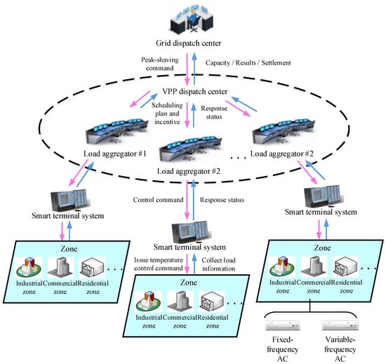
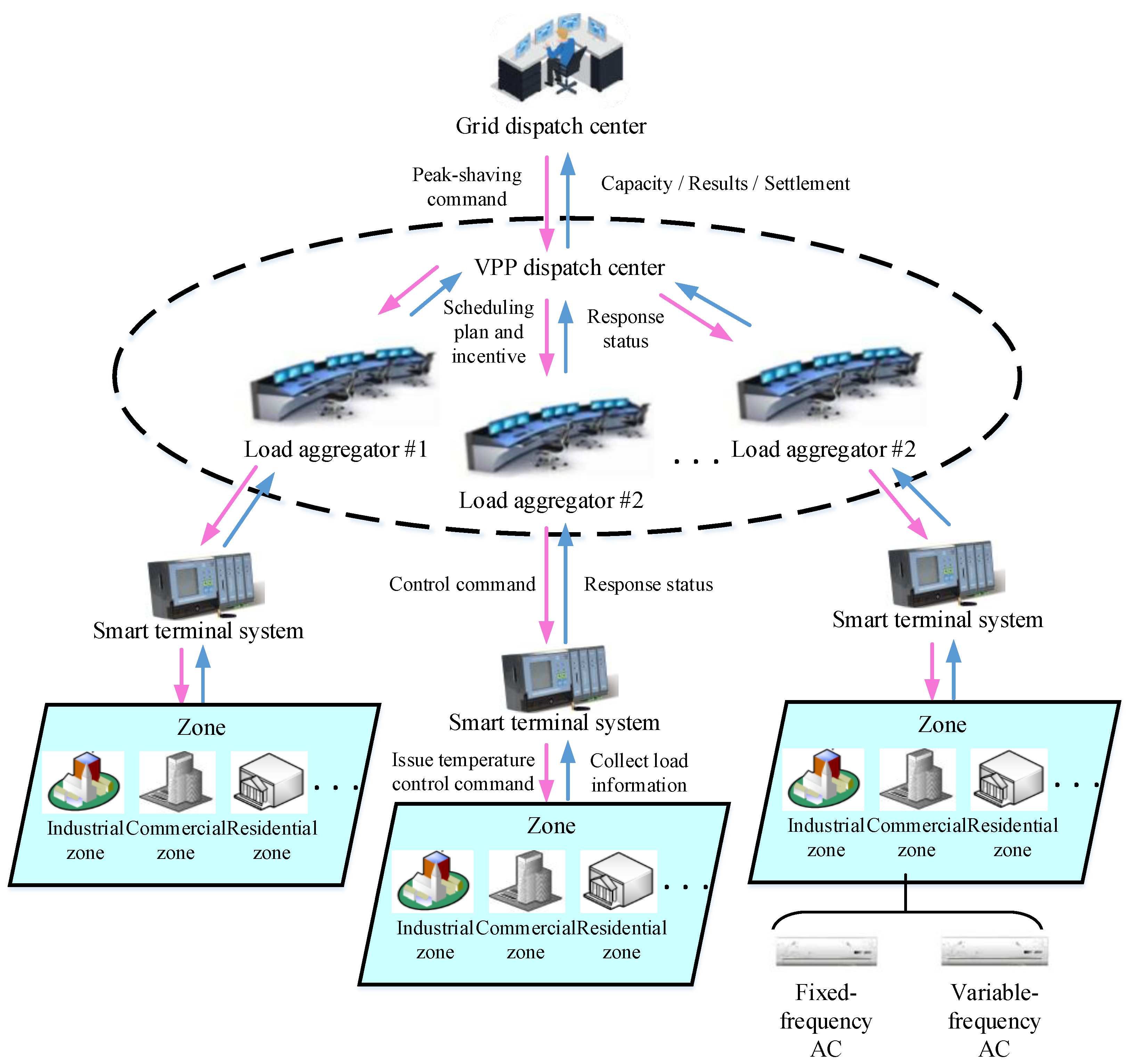
To address the limitations of conventional frameworks that utilize scheduling error as the sole objective, this paper proposes a multi-objective optimization scheduling strategy that explicitly incorporates both user satisfaction and revenue. The strategy employs a centralized optimization architecture, as illustrated in Figure 2. The grid dispatch center transmits peak-shaving commands to the VPP dispatch center, which subsequently issues peak-shaving instructions to each load aggregator within its jurisdiction. Each aggregator coordinates AC resources across industrial, commercial, and residential scenarios within its service area to develop localized capacity allocation and incentive schemes.
Figure 2.
Multi-objective optimal scheduling architecture for load-type VPP participation in peak-shaving services.
This paper focuses on an optimization model that addresses the multi-scenario co-scheduling problem within the jurisdiction of a single aggregator. In this framework, the load-type VPP simultaneously integrates the objectives of maximizing user revenue and minimizing user dissatisfaction, while ensuring precise tracking of peak-shaving commands. This co-optimization effectively aligns the peak-shaving requirements from the grid side with the interests of users. Accordingly, this section formulates the multi-objective optimization equations and, building on the subjective and objective constraint factors established in Section 2, defines appropriate capacity constraints.
- User Revenue
The revenue generated by AC users participating in peak-shaving services through load-type VPP consists of two components. The first component is the cost savings on electricity achieved by adjusting AC consumption during the peak-shaving period; if the adjusted cost exceeds the original cost, this component may become negative. The second component is the incentive income accrued from participating in VPP scheduling. From the user’s perspective, earning incentive income requires competing in a market with users from various scenarios within the VPP jurisdiction; a higher bid reduces the likelihood of securing a successful dispatch contract.
where is the revenue of AC users in scenario under day type from participating in peak-shaving services; is the incentive bid of users in scenario under day type (CNY/kWh); is the dispatch success probability at bid , as defined in Equation (37); is the electricity cost saved by the user during the peak-shaving period (positive when costs decrease and negative when costs increase); is the incentive income received from participating in VPP scheduling during ; is the real-time electricity price at time on the scheduling day (CNY/kWh); is the AC load adjustment at time ; is the time-step duration; and is the peak-shaving period.
The dispatch success probability is modeled as
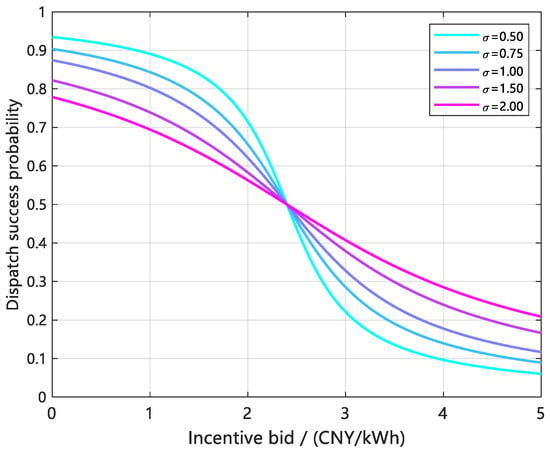
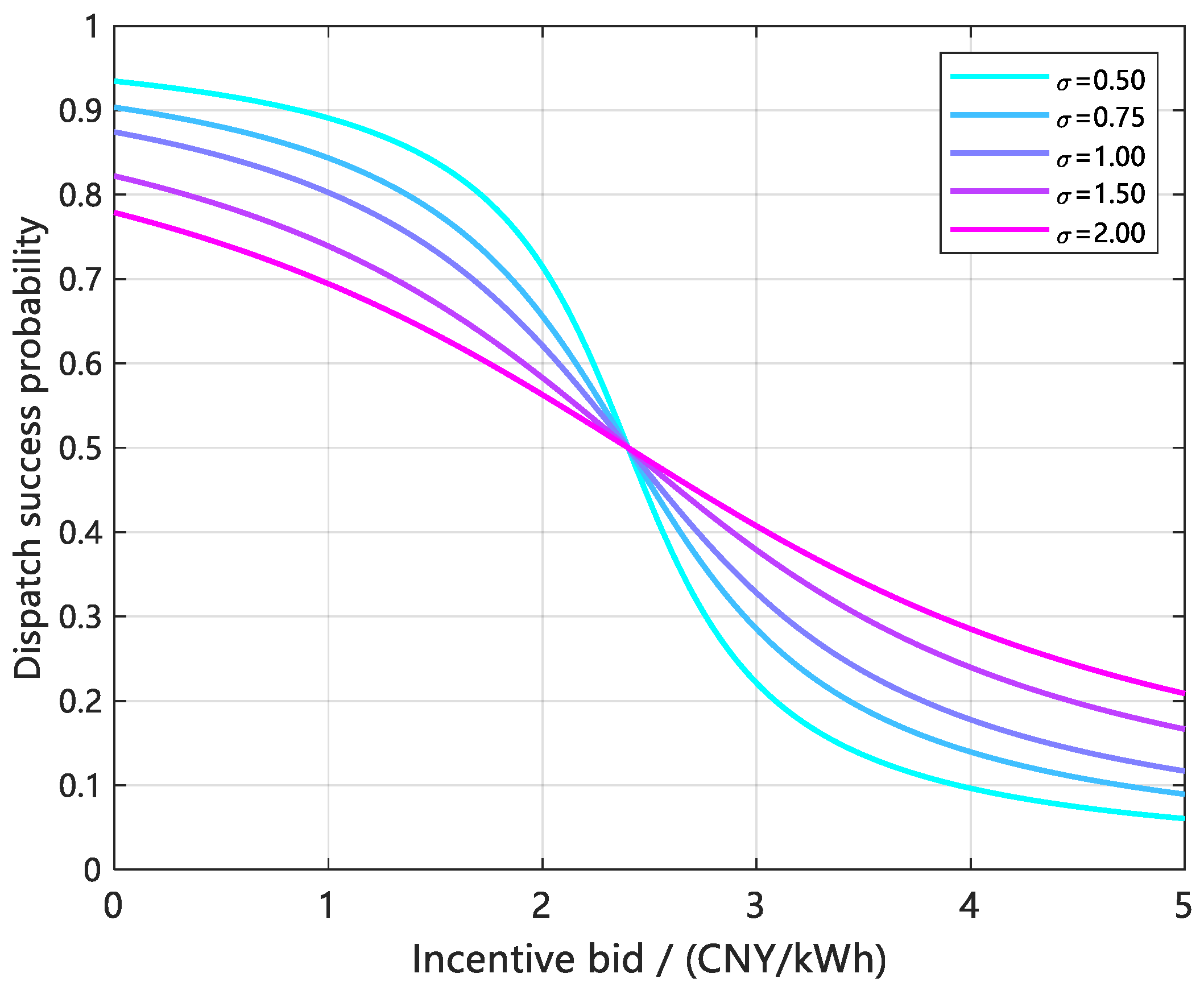
where is the reference bid corresponding to a 50% dispatch success probability (CNY/kWh); and is the price competition sensitivity coefficient reflecting the degree of market competition within the VPP jurisdiction.
- 2.
- User Satisfaction
According to consumer psychology theory, when the adjustment of AC power is minimal, user dissatisfaction increases only marginally with the extent of power reduction. However, as the adjustment becomes more significant, its effect on thermal comfort becomes increasingly pronounced. In scenarios where power reduction is substantial—approaching or reaching shutdown levels—user dissatisfaction peaks, and even a minor change in power can lead to a disproportionately large increase in dissatisfaction. These observations suggest that user dissatisfaction escalates nonlinearly with scheduled power adjustments and is particularly sensitive to changes in power within the high-adjustment range. Based on this analysis, the AC operating power, denoted as , is taken as the independent variable, and user dissatisfaction is modeled as
where is the user’s dissatisfaction with AC electricity usage in scenario under day type .
3.2. Objective Function Formulation
Assuming that the load-type VPP jurisdiction contains n scenarios, the scheduling capacity is allocated across scenarios to minimize the error between the total scheduling capacity and the peak-shaving command issued by the dispatch center, while jointly optimizing user satisfaction and revenue. The objective function is formulated as
where is the scheduling error for day type between the total scheduled capacity and the peak-shaving command; is the peak-shaving command issued by the dispatch center to the load-type VPP for day type during ; and is the scheduled AC load adjustment in scenario under day type .
For each scenario under day type , let denote the total scheduled capacity over the peak-shaving period. The weighted average dissatisfaction for each day type is defined as
where each scenario’s scheduled capacity share is taken as the weight.
Drawing on the scheduling response models for temperature-sensitive loads presented in Section 2.3 and Section 2.4, the upper and lower bounds on scheduling capacity are distinctly specified for each scenario based on the type of AC load.
- Curtailable AC loads
Considering user interaction willingness, the curtailable AC load must satisfy the elastic temperature adjustment range. The capacity bounds are
where denotes the set of curtailable load scenario indices; is the upper bound on scheduled capacity for curtailable AC load scenario under day type ; is the interaction willingness in scenario under day type at time , evaluated from Equation (23) based on the TOU price at period ; is the initial adjustable temperature range (i.e., the deadband width prior to regulation) in scenario at time ; and are the numbers of fixed-frequency and variable-frequency AC units in scenario , respectively; and , , and are the scenario- counterparts of , , and as defined in Equations (13) and (19), respectively.
- 2.
- Shiftable AC loads
The adjustable range of shiftable AC loads is determined by the fluctuation of the load transfer rate . The capacity bounds are
where denotes the set of shiftable load scenario indices; and are the upper and lower bounds on scheduled capacity for shiftable AC loads, obtained by substituting the upper limits () and lower limits () of the transfer rates , , and from Equations (31) and (32) into Equation (33), corresponding to the maximum and minimum feasible load shift amounts under the fuzzy uncertainty range, respectively.
3.3. Scheduling Strategy Solution Procedure
The model presented in this paper encompasses three optimization objectives. The decision variables are categorized into two dimensions: scheduling capacity and incentive pricing. Furthermore, both the relationship between the bid success rate and the bid price, as well as the relationship between user dissatisfaction and scheduled capacity, exhibit nonlinear characteristics. This leads to nonlinear coupling among the three objectives. Traditional algorithms, such as NSGA-II, encounter challenges related to reference surface degeneracy and struggle to maintain solution diversity when the number of objectives exceeds two. In contrast, NSGA-III introduces a structured reference-point mechanism that effectively preserves the uniform distribution of the Pareto front within the three-dimensional objective space. Consequently, NSGA-III is utilized to solve the model discussed in this paper.
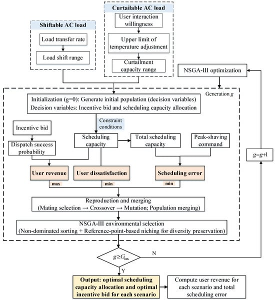
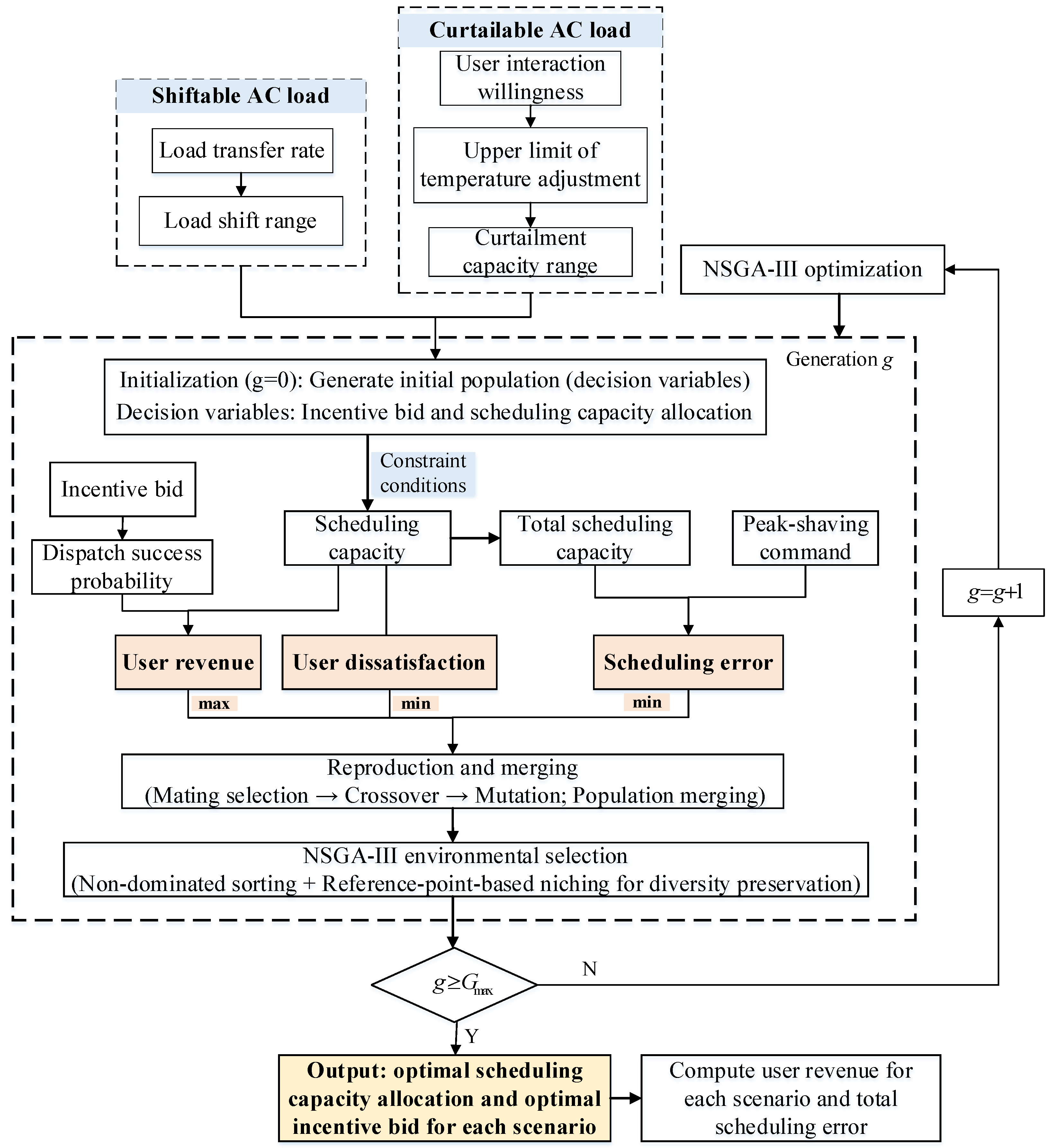
The NSGA-III algorithm is utilized to tackle the multi-objective scheduling problem for n AC load scenarios that participate in the peak-shaving ancillary service market under day type k, within the jurisdiction of the VPP. The solution procedure is illustrated in Figure 3 and is executed as follows.
Figure 3.
Solution procedure for the multi-objective optimal scheduling strategy integrating user satisfaction and revenue.
Step 1: Acquire scenario AC parameters and TOU pricing data. Compute the user’s willingness to interact and the upper limit of temperature adjustment for curtailable AC load scenarios, thereby determining the capacity upper bounds. Construct the corresponding feasibility constraints.
Step 2: Calculate the fluctuation range of the load transfer rate for shiftable AC load scenarios based on TOU data. Determine the capacity bounds for shiftable loads according to the peak-shaving periods specified by the dispatch center. Consolidate the capacity bounds and operating constraints for both curtailable and shiftable loads to establish the constraint conditions and feasibility criteria for the NSGA-III solver.
Step 3: With scenario-level capacity allocation and incentive bids as decision variables, we formulate a three-objective optimization model aimed at maximizing user revenue, minimizing user dissatisfaction, and minimizing scheduling errors. After initializing the population in NSGA-III, we apply selection, crossover, and mutation to generate offspring. This offspring is then merged with the parent population, followed by non-dominated sorting. Subsequently, we implement a reference point-based niching mechanism to iteratively maintain solution diversity until the Pareto-optimal solution set is achieved.
Step 4: Upon reaching the termination criterion, the NSGA-III algorithm outputs the Pareto-optimal solution set for one run. To reduce the influence of stochasticity, the NSGA-III procedure is independently repeated multiple times. After each run, the TOPSIS method is employed to select a unique compromise solution from the obtained Pareto set. The corresponding total user revenue, weighted average dissatisfaction, and scheduling error of the selected compromise solution are then recorded for subsequent statistical analysis and result reporting.
4. Case Study
4.1. Scenario Description
The VPP service area is categorized into three distinct scenarios: a residential zone, a commercial zone, and a large industrial zone. In the large industrial zone, controllable AC loads are represented as shiftable loads, while those in the residential and commercial zones are characterized as curtailable loads. Both weekdays () and non-weekday days () are taken into account. To reduce computational complexity, a simplified distribution network configuration is adopted in the case study, following prior studies [24]. The AC parameters for each scenario, adapted from Ref. [15], along with the TOU prices for each type of day based on the TOU tariff of a city in eastern China, are presented in Table 1 and Table 2, respectively. According to the current VPP subsidy policy in Jiangsu Province, the incentive bidding range for all three scenarios is established at 0–4.8 CNY/kWh, with the reference bid , which corresponds to a 50% success rate, set at 2.4 CNY/kWh. In the benchmark strategy (Strategy 1), the scenarios participate through a conventional load aggregator, and the incentive bid remains fixed at 2.4 CNY/kWh across all scenarios. In the proposed joint optimization strategy (Strategy 2), the incentive bids and scenario-level scheduling capacities are jointly optimized using the multi-objective model developed in Section 3.
Table 1.
Scenario AC parameters.
Table 2.
TOU pricing and baseline prices by scenario.
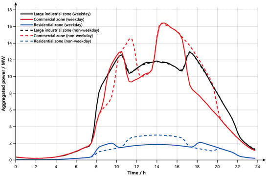
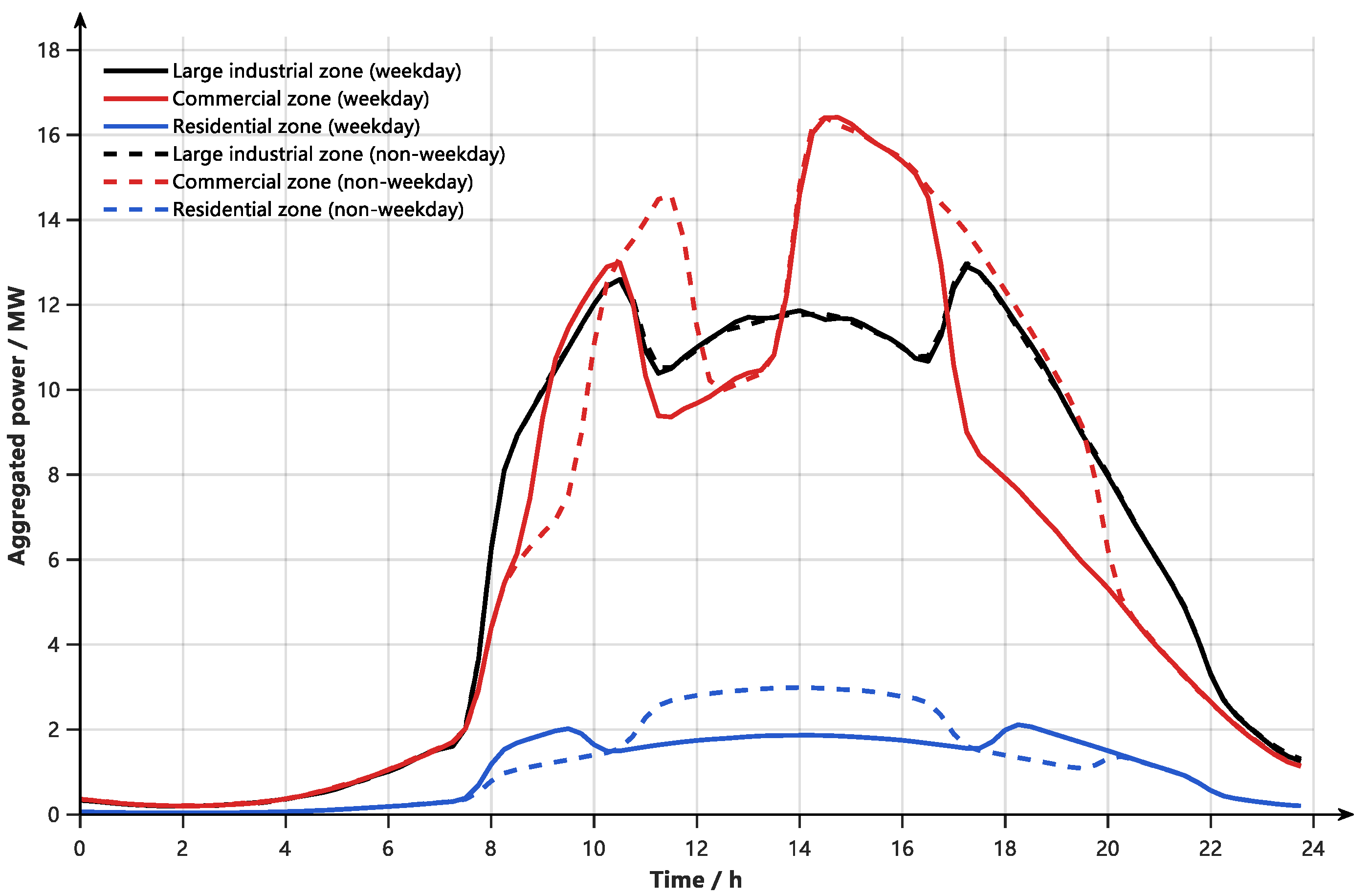
Based on the AC equipment parameters in Table 1, the aggregated AC load curves of the three scenarios are obtained through Monte Carlo aggregation, as shown in Figure 4.
Figure 4.
Daily aggregated power curves of the combined fixed- and variable-frequency AC fleets across three scenarios under two-day types.
Figure 4 illustrates the 24 h aggregated power curves for the combined fixed- and variable-frequency AC fleets across all three scenarios, considering both types of days. The commercial zone on weekdays exhibits a double-peak profile within the 10:00–20:00 window, reaching a peak of approximately 16.4 MW. In contrast, the large industrial zone maintains relatively stable power levels between 11 and 13 MW throughout the day, with a variation in less than 1 MW between weekdays and non-weekdays. The residential zone shows a daily aggregated power range of 0.3–2.5 MW, featuring a single peak of approximately 2.5 MW occurring between 13:00 and 16:00.
The amplification coefficients for the large industrial zone are . For the commercial zone, reduced foot traffic on non-weekdays lowers price sensitivity relative to weekdays, so = 1.5 and = 1. For the residential zone, . For ease of analysis, the interaction willingness values are categorized into four states: denotes a negative willingness; denotes a neutral state; denotes a moderately positive willingness; and denotes a strongly positive willingness.
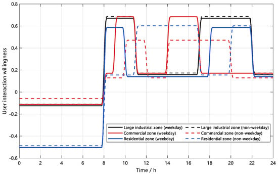
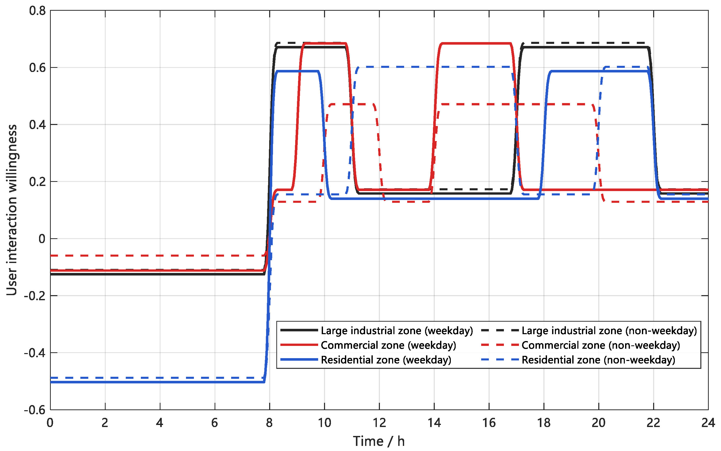
The computed 24 h willingness curves are illustrated in Figure 5. Taking weekdays as an example, the large industrial zone experiences peak electricity demand between 08:00 and 11:00, as well as from 17:00 to 22:00, coinciding with peak TOU periods, where the willingness peaks at 0.671, indicating a strongly positive response. In contrast, the commercial zone’s peak prices occur during business hours, specifically from 10:00 to 12:00 and 14:00 to 20:00, resulting in a willingness peak of 0.684, which is also strongly positive. The residential zone, influenced by commuting patterns, concentrates electricity usage between 08:00 and 10:00, and from 18:00 to 22:00, with a willingness peak of 0.596, categorized as moderately positive. Regarding differences between day types, the large industrial zone shows no significant variation in peak willingness periods or magnitudes between weekdays and non-weekdays. Conversely, the commercial zone exhibits a notably lower willingness on non-weekdays, with the maximum dropping from strongly positive to moderately positive. The residential zone shifts its peak willingness window to 11:00 to 17:00 and from 20:00 to 22:00 on non-weekdays, although the magnitude remains comparable to that observed on weekdays. These time-varying willingness profiles serve as the subjective input for the curtailable load constraints discussed in Section 4.2.
Figure 5.
24 h user interaction willingness curves across three scenarios under two-day types.
The NSGA-III is configured with a population size of 100, a maximum of 500 generations, a mutation rate of 0.15, and 12 reference point divisions for three objectives. A total of 20 independent runs are performed, and the final solution is selected using the TOPSIS compromise method.
4.2. Scheduling Capacity Constraint Calculation
4.2.1. Shiftable Load Constraints for the Large Industrial Zone
From the TOU pricing in Table 2 for the large industrial zone, the price differentials are computed as: peak-to-valley = 0.819 CNY/kWh, peak-to-flat = 0.453 CNY/kWh, and flat-to-valley = 0.366 CNY/kWh. The load transfer rate model parameters in Table 3 are determined empirically based on engineering practice. Substituting these values along with the model parameters in Table 3 into Equations (31)–(33), the load shift fluctuation ranges for each period are obtained, as shown in Table 4.
Table 3.
Load transfer rate model parameters for the large industrial zone.
Table 4.
Load shift fluctuation ranges for each period in the large industrial zone.
Table 4 demonstrates that at the upper transfer rate limit, 1221.56 kW and 250.33 kW are transferred from peak and flat periods to valley periods, respectively. Conversely, at the lower transfer rate limit, 902.89 kW and 185.03 kW are similarly shifted from peak and flat periods to valley periods.
4.2.2. Curtailable Load Constraints for the Commercial and Residential Zones
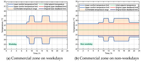
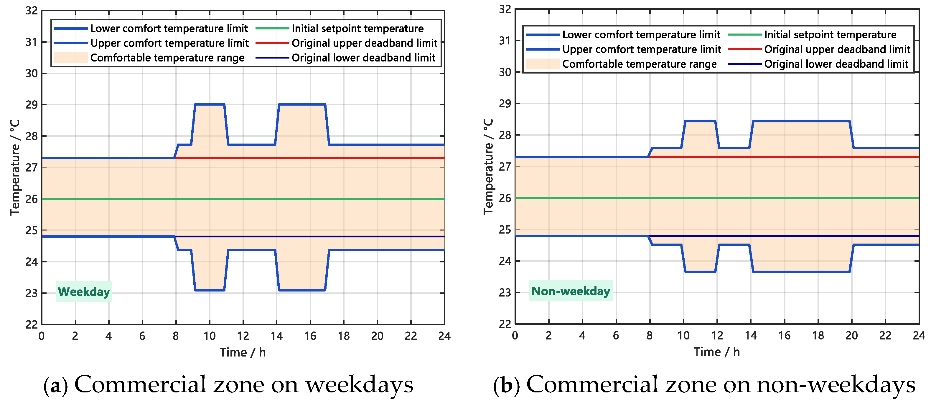
A typical summer daily temperature curve for Jiangsu Province is adopted. The initial setpoint temperature for all three scenarios is assumed to be 26 °C. Based on the optimal thermal comfort index range for human occupants, a comfortable indoor temperature range of 24.8–27.3 °C is adopted as the initial adjustable temperature interval. Taking the commercial zone as an example, Figure 6 illustrates the full-day variation in the elastic temperature adjustment range on both weekdays and weekends. By utilizing the interaction willingness values from Table 5 and applying Equation (24), the upper limits for elastic temperature adjustments are determined for each scenario. The resulting upper bounds on air conditioning load curtailment for both the commercial and residential zones across different day types are presented in Table 5.
Figure 6.
Elastic temperature adjustment range for the commercial zone.
Table 5.
Upper bounds on AC load curtailment for the commercial and residential zones.
Table 5 indicates that the upper bound for weekday commercial-zone peak curtailment (5707.35 kW) is 49.9% greater than the corresponding non-weekday value (3804.90 kW) for the same period. The willingness ratio between the two is 1.50, and this proportional relationship extends to the capacity bounds through the linear mapping defined in Equation (24). Notably, the peak curtailment upper bound for the residential zone remains consistent across both weekdays and non-weekdays at 1059.93 kW. This finding aligns with Equation (23), as the peak-to-valley price differential is 0.28 CNY/kWh on both types of days, resulting in identical willingness values. Across various scenarios, the peak-period curtailment upper bound is approximately 3.5 to 4.0 times the flat-period value, underscoring the impact of TOU price incentive differentials on scheduling capacity constraint boundaries.
4.3. Scheduling Strategy and Results Analysis
Three representative peak-shaving periods are selected for the case study: weekday afternoon (14:00–15:00) with a command of 4.2 MW, weekday evening (19:00–20:00) with 2.5 MW, and non-weekday afternoon (14:00–15:00) with 3.5 MW. For each period, Strategy 2 is compared against Strategy 1 in terms of capacity allocation, user revenue, and user dissatisfaction. The scheduling time resolution is set to 15 min.
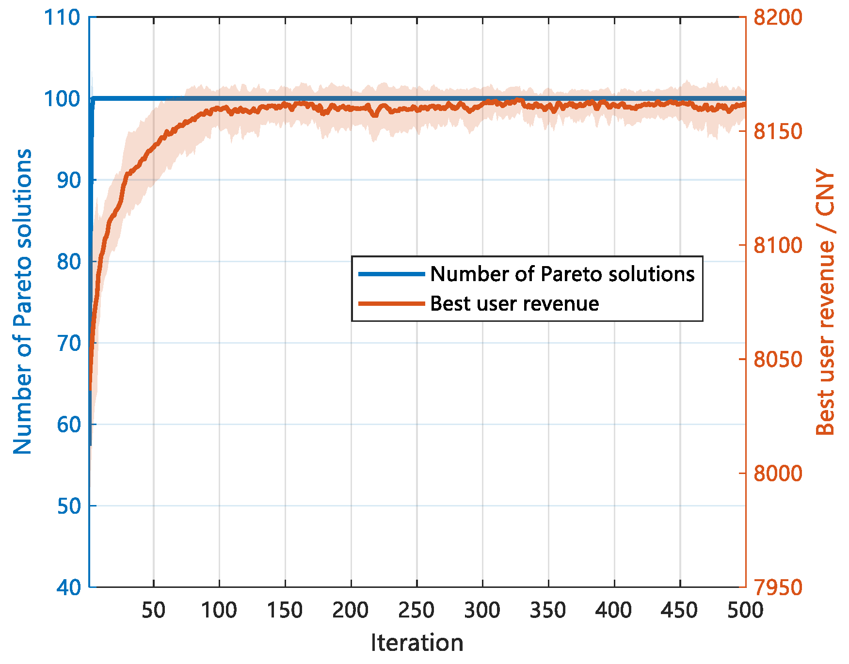
Before comparing the two scheduling strategies in detail, the convergence performance of the optimization algorithm is first illustrated for a representative peak-shaving period. Figure 7 shows the mean convergence curve and standard deviation of 20 independent NSGA-III runs for the weekday 14:00–15:00 period. The results indicate that the algorithm converges rapidly and remains stable in the later iterations, demonstrating good convergence and robustness over repeated runs.
Figure 7.
Convergence behavior of NSGA-III over 20 independent runs.
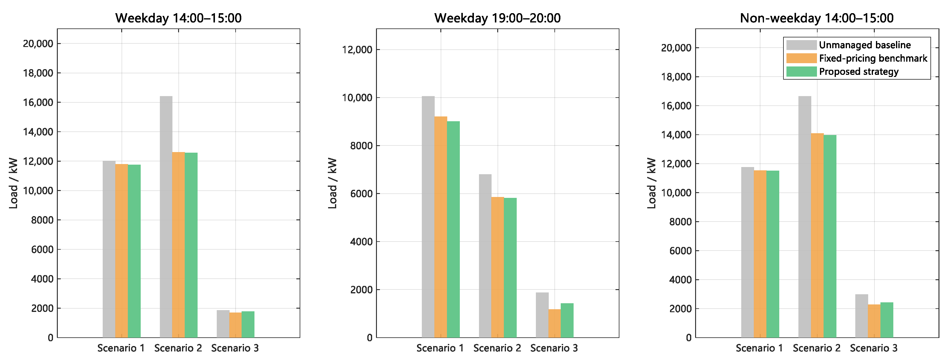
Figure 8 further presents the scenario-level AC loads under the unmanaged baseline, the fixed-pricing benchmark (Strategy 1), and the proposed strategy (Strategy 2) during the three representative peak-shaving periods. The unmanaged baseline represents the natural AC demand without coordinated scheduling, while the two scheduled strategies show how this demand can be redistributed and reduced across scenarios to provide peak-shaving response.
Figure 8.
Scenario-level AC loads under the unmanaged baseline, Strategy 1, and Strategy 2 across three peak-shaving periods.
As shown in Figure 8, both strategies reduce the AC load in each scenario relative to the unmanaged baseline. Although the overall peak-shaving task is similar, the differences in scenario-level load reduction between Strategy 1 and Strategy 2 indicate distinct capacity allocation patterns, which are further examined in the following subsections from the perspectives of capacity allocation, user revenue, and user dissatisfaction.
- Optimal Capacity Allocation and Incentive Bids
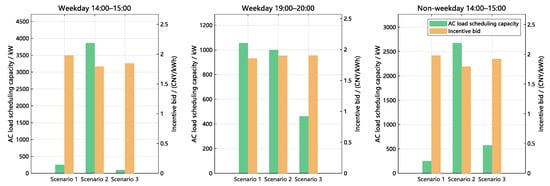
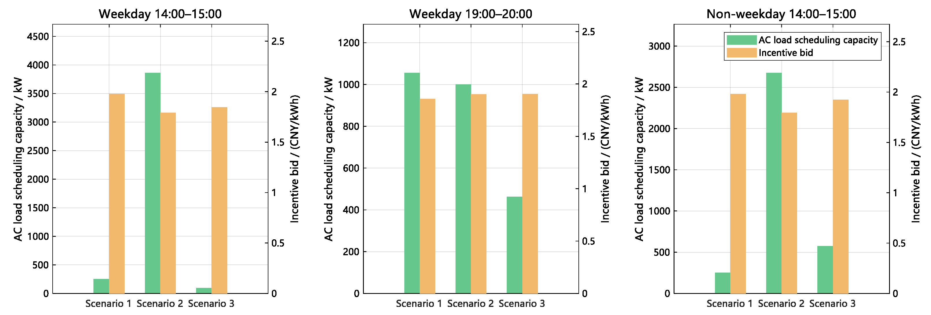
As illustrated in Figure 9, the capacity allocation patterns across the three peak-shaving periods exhibit a distinct dependence on the time of day. During the weekday period from 14:00 to 15:00, Strategy 2 predominantly allocates capacity to Scenario 2 (commercial zone), with a scheduled capacity of approximately 3850 kW, accounting for 91.7% of the total. In contrast, Scenario 1 (large industrial zone) and Scenario 3 (residential zone) receive approximately 250 kW (5.9%) and 100 kW (2.4%), respectively. The incentive bids for the three scenarios are approximately 2.0, 1.7, and 1.8 CNY/kWh, all of which are below the fixed benchmark of 2.4 CNY/kWh. During the weekday period from 19:00 to 20:00, all three scenarios experience their respective peak-price periods, with the differences in willingness to pay being smaller compared to the earlier time period.
Figure 9.
Optimal AC load scheduling capacity and incentive bids for each scenario across three peak-shaving periods.
Strategy 2 allocates approximately 1050 kW (42.0%), 1000 kW (40.0%), and 460 kW (18.4%) across the three scenarios, resulting in a more balanced distribution. The incentive bids for all scenarios are approximately 1.9 CNY/kWh, with inter-scenario differences remaining below 0.1 CNY/kWh. During the non-weekday period from 14:00 to 15:00, the large industrial zone experiences a flat load period, compressing its shiftable load capacity upper bound to 250.33 kW, thus Scenario 1 receives approximately 250 kW (7.1%). The curtailment upper bound for the commercial zone (3804.90 kW) is 3.6 times greater than that of the residential zone (1059.93 kW); consequently, Strategy 2 allocates approximately 2700 kW (77.1%) to Scenario 2 and approximately 570 kW (16.3%) to Scenario 3. The bid for the commercial zone is approximately 1.8 CNY/kWh, while the bid for the residential zone is approximately 2.0 CNY/kWh.
- 2.
- Comparison of Scheduling Capacity by Scenario
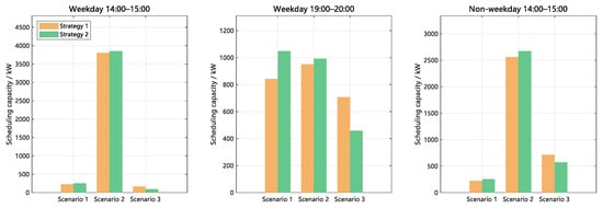
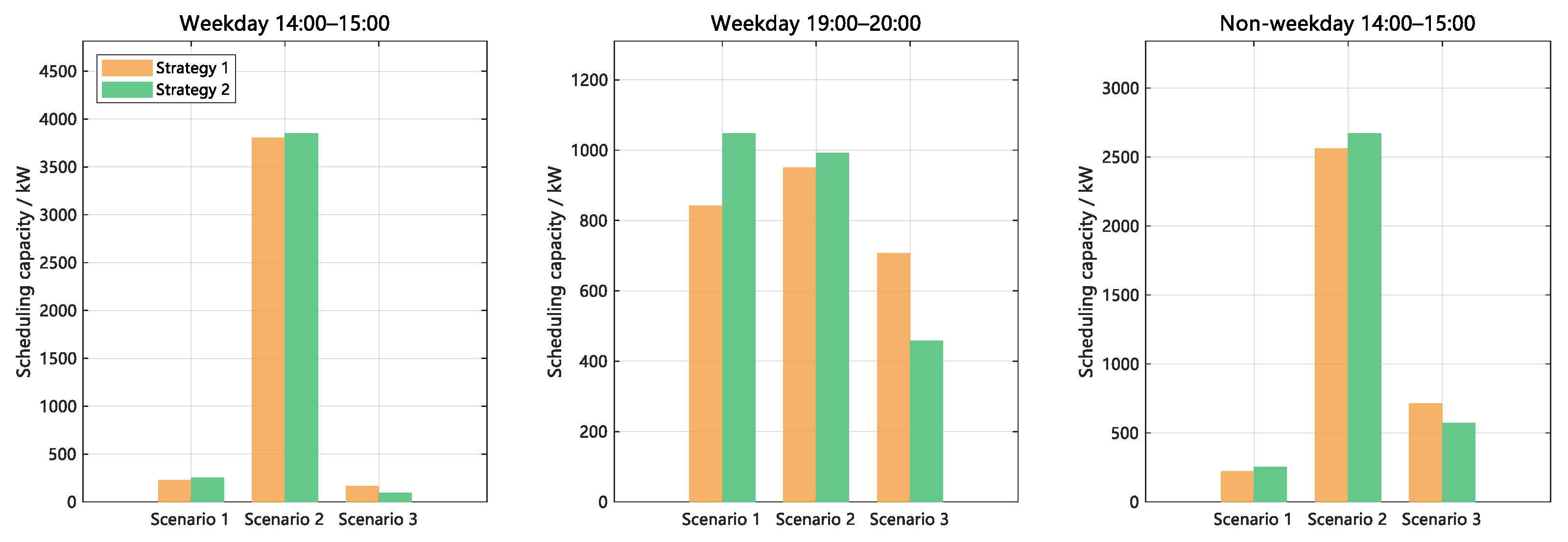
As can be seen from Figure 10, Strategy 2 alters the capacity allocation pattern compared to Strategy 1 across all three periods. During weekdays from 14:00 to 15:00, capacity is significantly concentrated in Scenario 2, while Scenarios 1 and 3 experience reduced allocations. In the weekday period from 19:00 to 20:00, allocations for Scenarios 1 and 2 increase, whereas Scenario 3 encounters a slight decrease. During non-weekdays from 14:00 to 15:00, Scenario 2 receives an increased allocation, and Scenario 3 is allocated less; Scenario 1 remains consistently allocated under both strategies due to its binding flat-period capacity upper bound.
Figure 10.
Comparison of scheduling capacity by scenario for Strategy 1 and Strategy 2 across three peak-shaving periods.
- 3.
- Comparison of User Revenue
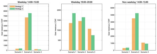
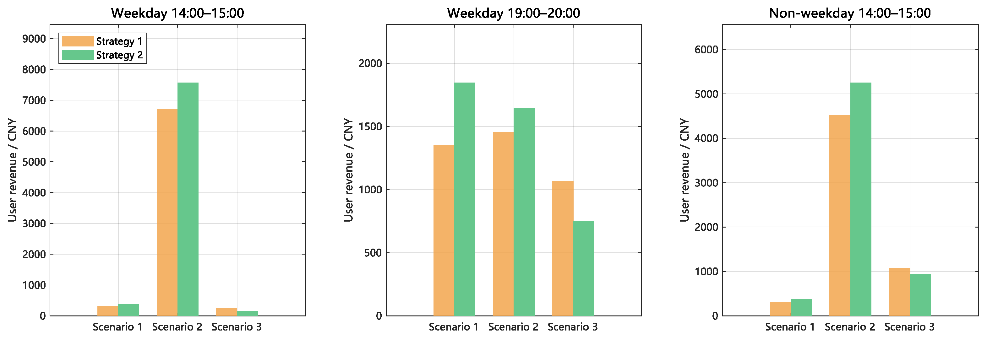
As illustrated in Figure 11, Strategy 2 consistently generates higher total revenue than Strategy 1 across all three periods, although the direction of revenue changes for individual scenarios varies based on the capacity allocation pattern. During weekdays from 14:00 to 15:00, Strategy 2 allocates capacity predominantly to Scenario 2, which increases its revenue from approximately 6700 CNY to around 7600 CNY. Conversely, Scenarios 1 and 3 experience a decline in revenue due to reduced allocated capacities. Consequently, total user revenue across all three scenarios rises from 7267.1 CNY to 8092.6 CNY, reflecting an improvement of 11.4%. During the weekday period from 19:00 to 20:00, all three scenarios are subjected to peak pricing with minimal differences in willingness to pay; the balanced allocation leads to revenue increases across all scenarios, resulting in a total revenue enhancement of 9.4%. In the non-weekday period from 14:00 to 15:00, total revenue escalates from 5901.0 CNY to 6562.8 CNY, marking a gain of 11.2%.
Figure 11.
Comparison of user revenue by scenario for Strategy 1 and Strategy 2 across three peak-shaving periods.
- 4.
- Comparison of User Dissatisfaction
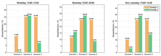
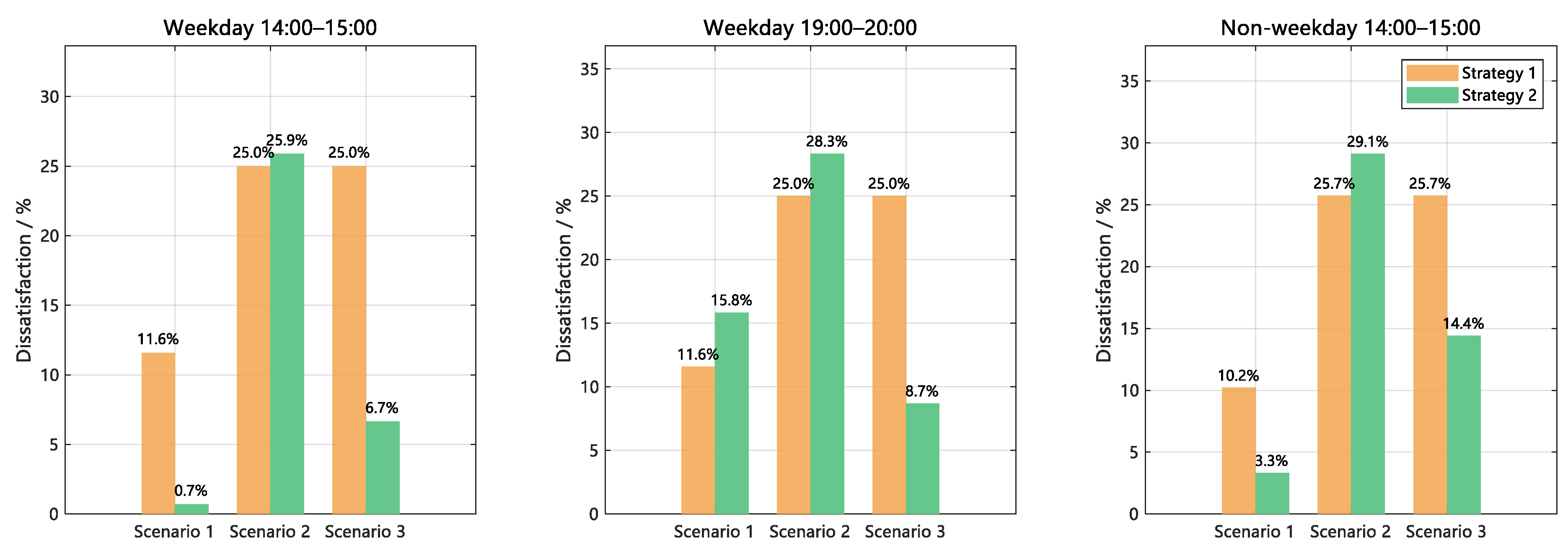
As illustrated in Figure 12, the shifts in dissatisfaction across various scenarios directly correlate with the capacity allocation patterns. Scenarios that experience reduced dispatch exhibit lower levels of dissatisfaction, whereas those that receive concentrated capacity increases demonstrate heightened dissatisfaction. Specifically, during the weekday period from 14:00 to 15:00, substantial reductions in Scenarios 1 and 3 result in notable decreases in dissatisfaction. In contrast, Scenario 2, which accommodates the concentrated capacity, experiences a slight uptick in dissatisfaction. Conversely, during the weekday period from 19:00 to 20:00, the increased allocations to Scenarios 1 and 2, compared to Strategy 1, lead to a rise in their dissatisfaction levels, while the diminished allocation to Scenario 3 contributes to a reduction in dissatisfaction. The non-weekday period from 14:00 to 15:00 exhibits a similar trend to the initial period: Scenario 2, which receives the highest dispatch share, sees a slight increase in dissatisfaction, while both Scenarios 1 and 3 experience declines in dissatisfaction.
Figure 12.
Comparison of user dissatisfaction by scenario for Strategy 1 and Strategy 2 across three peak-shaving periods.
Across all three peak-shaving periods, Strategy 2 enhances total user revenue by 9.4% to 11.4% and decreases the weighted average dissatisfaction by 0.27 to 1.92 percentage points compared to Strategy 1. It is important to note that Strategy 2 is primarily designed for overall revenue maximization. In specific periods, it may compress the dispatch of scenarios with stricter capacity constraints, resulting in a decline in revenue for those individual scenarios. This phenomenon represents a structural characteristic of the inter-scenario trade-off within the multi-objective framework. From the perspective of overall VPP operations, the proposed framework achieves a net increase in total revenue while ensuring the accuracy of peak-shaving command tracking. The extent of improvement in weighted dissatisfaction is influenced by both the capacity constraint configurations and the time-varying willingness profiles for each period.
4.4. Internal Model Comparison of Differentiated Pricing and Sensitivity Analysis
4.4.1. Internal Model Comparison of Differentiated Pricing
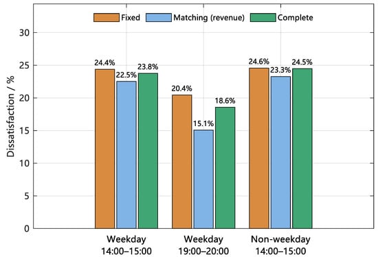
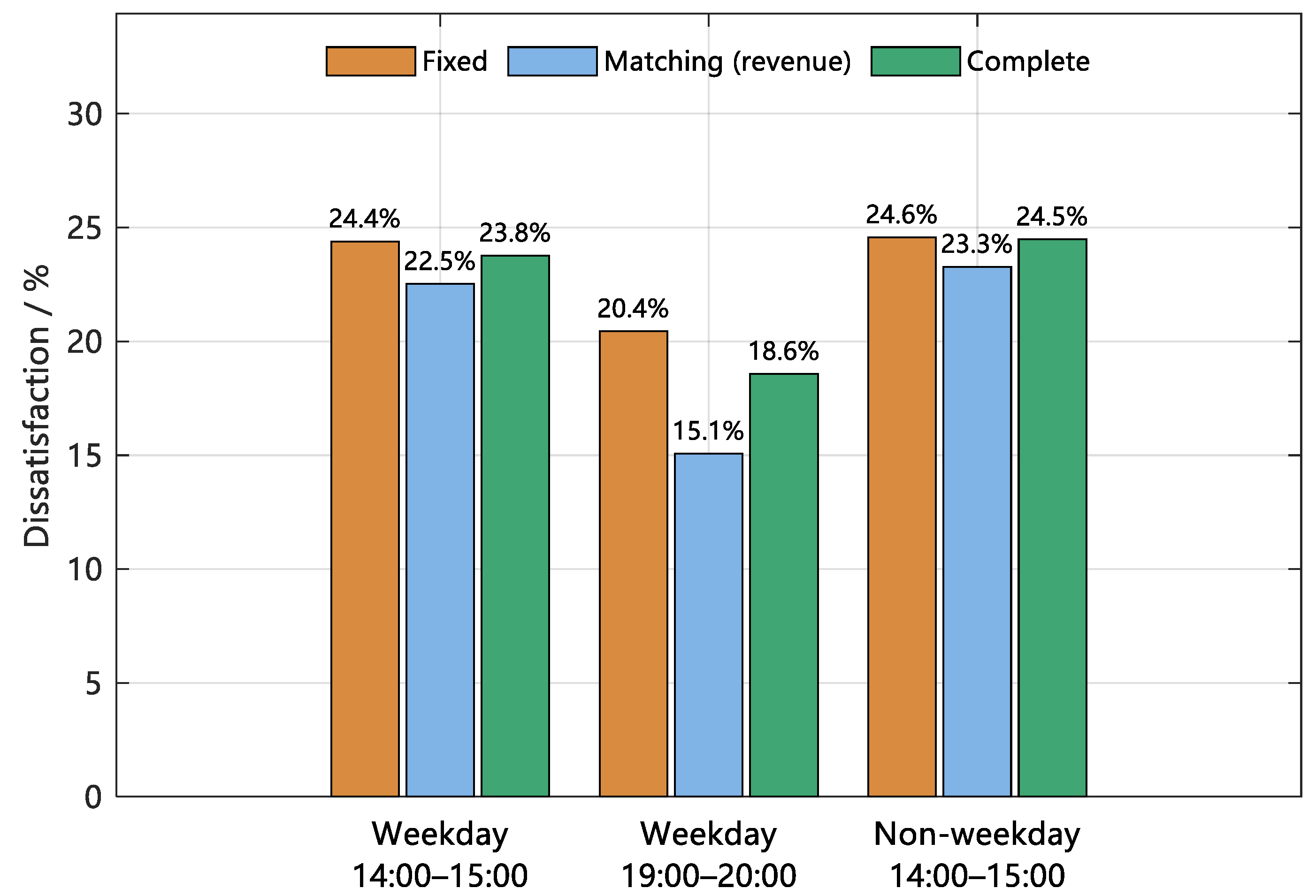
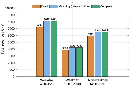
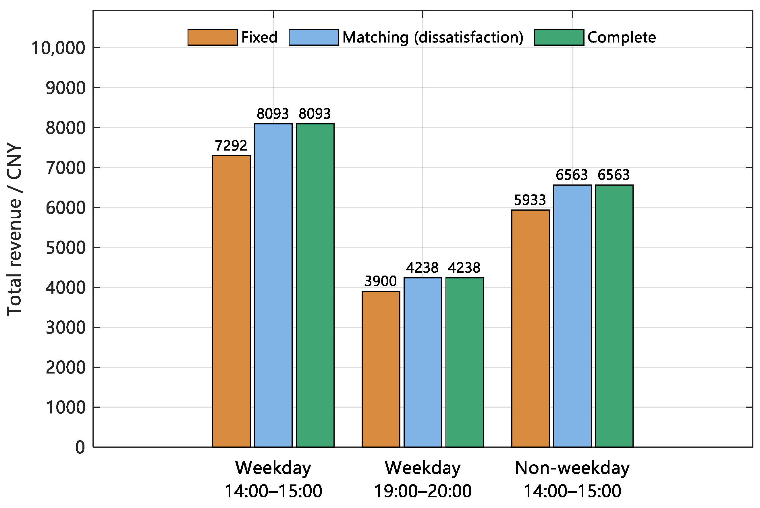
To isolate the contribution of differentiated pricing within the present model and case study settings, three internal comparison schemes are constructed as variants of Strategy 2, differing sorely in the extent to which scheduling capacity and incentive bid are jointly optimized. All three schemes are implemented within the NSGA-III framework and therefore differ from Strategy 1, which fixes the incentive price at 2.4 CNY/kWh and allocates capacity proportionally without optimization, serving only as an external benchmark. The Fixed scheme constrains to 2.4 CNY/kWh and optimizes only capacity allocation. The Matching scheme retains differentiated pricing but imposes an additional scalar constraint: in Figure 11, a revenue lower bound equal to the Fixed-scheme baseline is enforced, and the solution with the lowest weighted dissatisfaction is selected from the feasible Pareto subset; in Figure 13, a dissatisfaction upper bound equal to the Fixed-scheme baseline is enforced, and the solution with the highest total revenue is selected. The Complete scheme simultaneously optimizes both decision dimensions without additional scalar constraints and is equivalent to Strategy 2.
Figure 13.
Comparison of weighted dissatisfaction across schemes under the revenue constraint.
Figure 13 demonstrates that, while ensuring that the total revenue does not fall below the Fixed scheme baseline, the Complete scheme achieves lower weighted dissatisfaction than the Fixed scheme across all three periods, with reductions ranging from 4.0 to 7.9 percentage points. The Matching scheme exhibits some improvement over the Fixed scheme only during the weekday 14:00–15:00 period; in the other two periods, it shows little difference from the Fixed scheme. These results indicate that, under a fixed bid, merely applying NSGA-III optimization to capacity allocation is insufficient to achieve the dissatisfaction reductions realized by the Complete scheme. Differentiated pricing leads to a more significant reduction in dissatisfaction during the weekday 19:00–20:00 and non-weekday 14:00–15:00 periods.
As illustrated in Figure 14, under the constraint that weighted dissatisfaction does not exceed the baseline established by the Fixed scheme, both the Matching scheme and the Complete scheme achieve identical total revenues across all three periods, surpassing the Fixed scheme by 8.7% to 10.8%. The Fixed scheme fails to attain this revenue level while complying with the dissatisfaction baseline constraint. This finding demonstrates that, within the context of the present case study, the integration of differentiated pricing into joint optimization is more effective for enhancing total revenue than merely fixing the price and optimizing capacity allocation.
Figure 14.
Comparison of total revenue across schemes under the dissatisfaction constraint.
4.4.2. Sensitivity Analysis
Single-factor sensitivity analyses are conducted for two key model parameters: the price competition sensitivity coefficient in Equation (37), which reflects the degree of market competition, and the user interaction willingness amplification coefficient in Equation (23), which captures the effects of non-price factors.
As shown in Figure 15, the coefficient governs the slope of the dispatch success rate as a function of the bid deviation from the reference value. Values of = 0.5, 0.75, 1.0, 1.5 and 2.0 are tested for during the weekday period from 14:00 to 15:00. Figure 13 shows that all five curves intersect at a 50% success rate at the reference bid of 2.4 CNY/kWh. A smaller produces a steeper curve and a wider modulation range for differentiated pricing.
Figure 15.
Family of dispatch success rate curves.
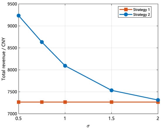
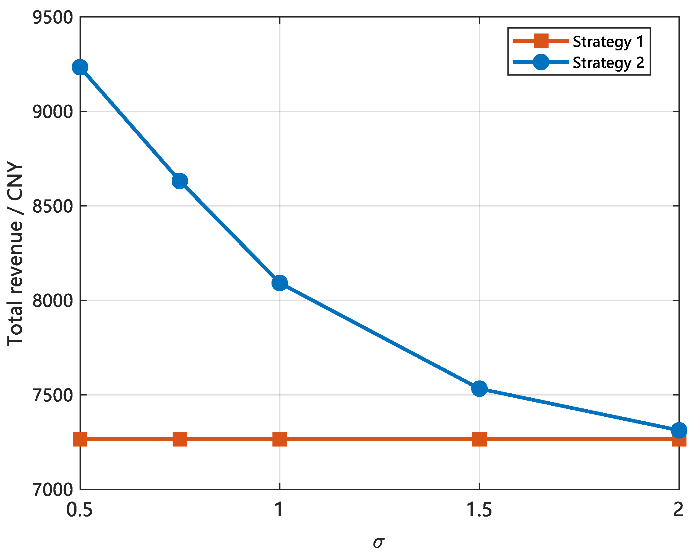
As shown in Figure 16, Strategy 1 uses a fixed bid, maintaining a constant of 0.5, resulting in total revenue that remains approximately stable at around 7300 CNY, irrespective of . In contrast, the total revenue of Strategy 2 exhibits a monotonically decreasing trend as increases, declining from approximately 9250 CNY at = 0.5 to about 7300 CNY at = 2.0. The revenue improvement relative to Strategy 1 diminishes from roughly 26.7% to approximately 0.7%. This decline can be directly attributed to the flattening of the success-rate curve as increases, which reduces the modulation range that differentiated pricing can exploit.
Figure 16.
Total revenue as a function of the price competition sensitivity coefficient
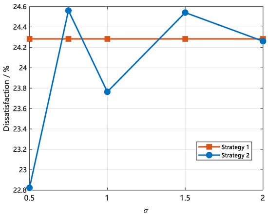
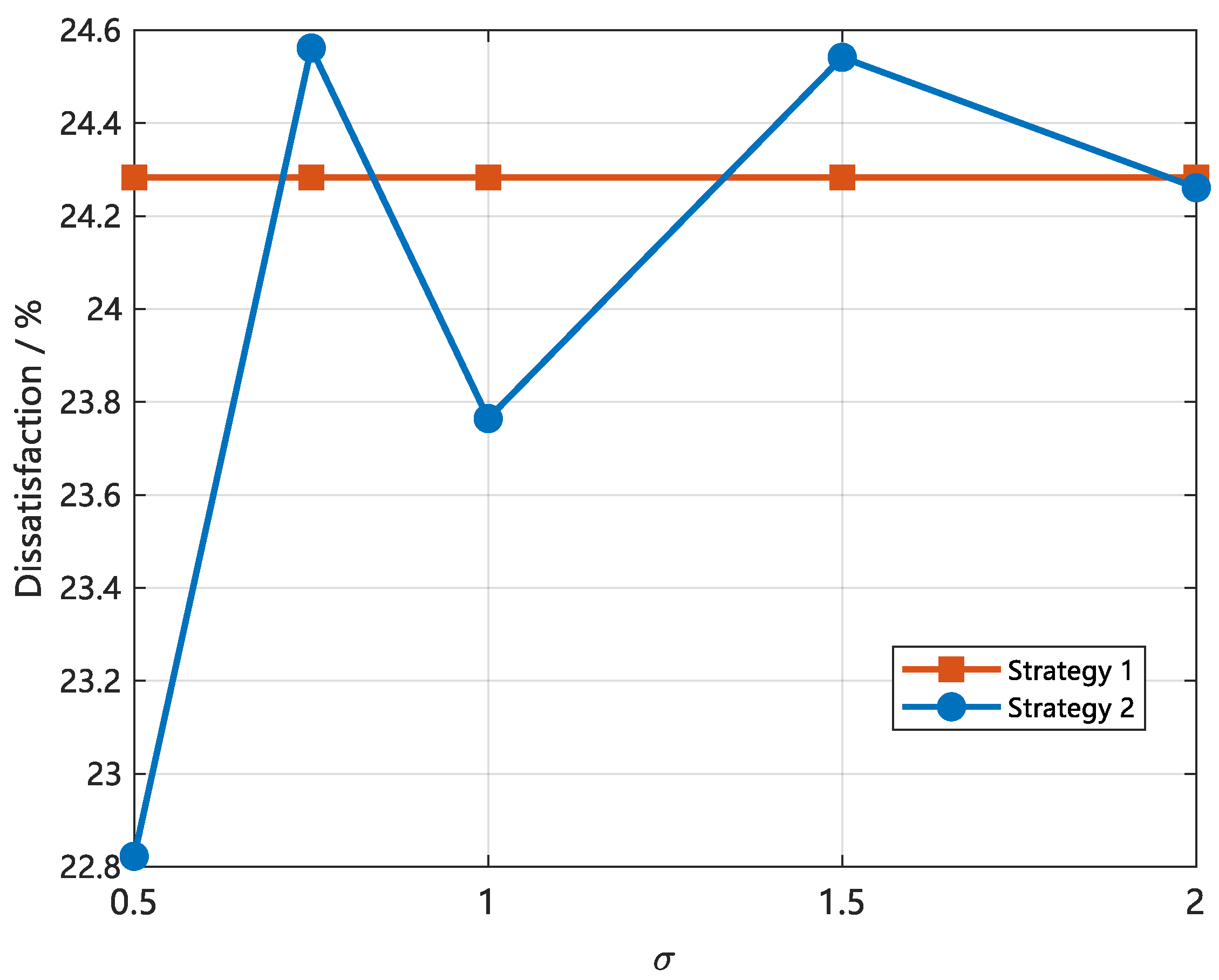
As shown in Figure 17, the dissatisfaction associated with Strategy 1 is stable at approximately 24.3% across all values of , which is consistent with its fixed bid and unchanging capacity allocation pattern. In contrast, the dissatisfaction of Strategy 2 varies non-monotonically with , exhibiting local peaks at = 0.75 and = 1.5. These results indicate that within the current model and case study, the enhancement of dissatisfaction associated with differentiated pricing is more effectively achieved at smaller values of . As increases, this improvement becomes less pronounced in the model output.
Figure 17.
Weighted dissatisfaction as a function of the price competition sensitivity coefficient
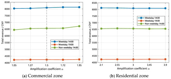
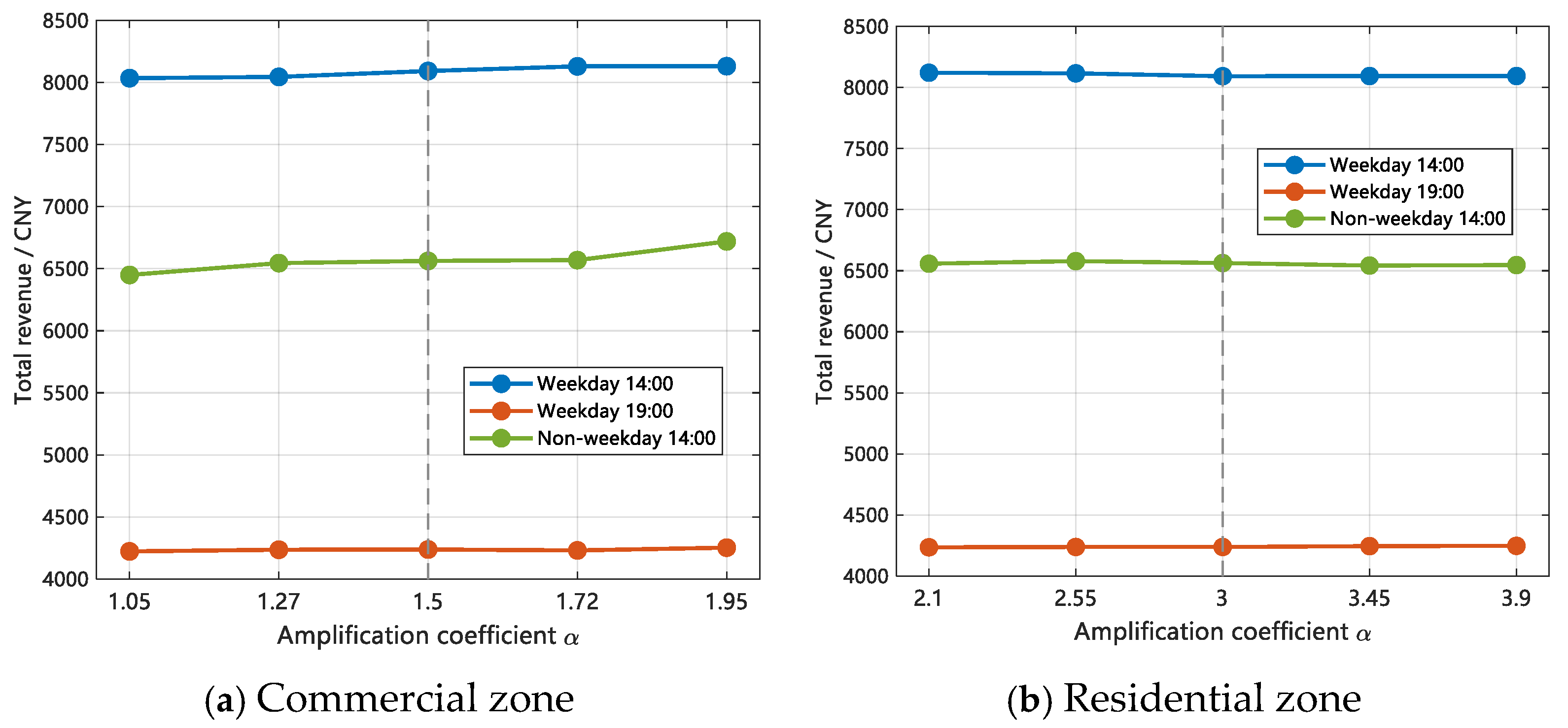
The amplification coefficient affects the allowable temperature adjustment range and the upper bound of curtailable capacity, as defined in Equation (24). Single-factor sensitivity analyses are performed separately for the commercial and residential zones, with set to 0.7, 0.85, 1.0, 1.15, and 1.3 times the respective baseline values. As shown in Figure 18, as varies within this range, the total revenue over the three peak-shaving periods changes by no more than 3%. This indicates that revenue is mainly determined by the total scheduled capacity and the bid level, whereas the direct effect of is limited.
Figure 18.
Total revenue as a function of the user interaction willingness amplification coefficient The dashed line indicates the baseline value of
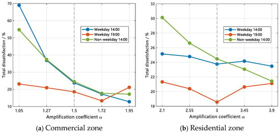
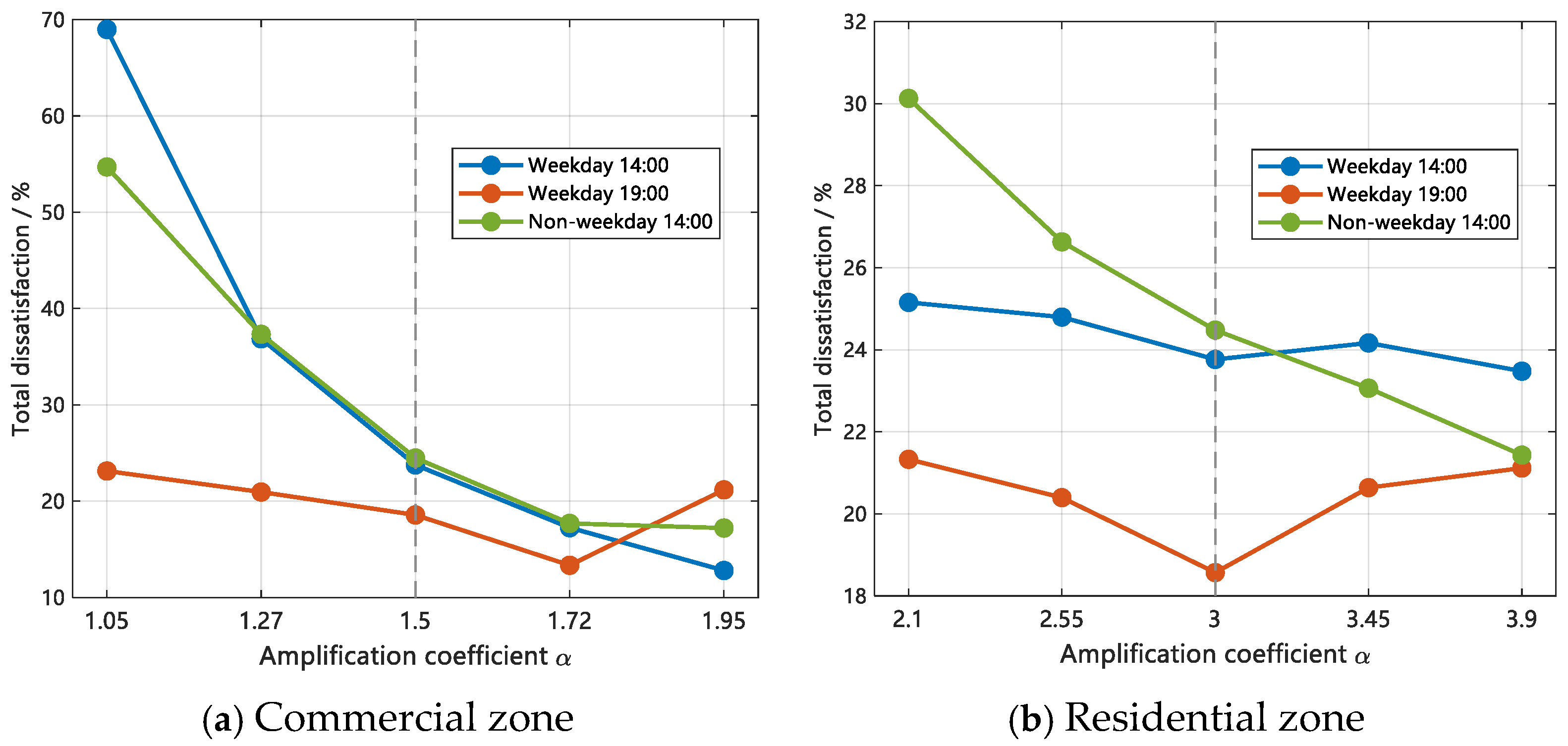
As illustrated in Figure 19, dissatisfaction exhibits a significantly greater sensitivity to change compared to revenue. In the commercial zone, when increases from 1.05 to 1.95, dissatisfaction during both the weekday period of 14:00–15:00 and the non-weekday period of 14:00–15:00 decreases by more than 40%.
Figure 19.
Weighted dissatisfaction as a function of the user interaction willingness amplification coefficient The dashed line indicates the baseline value of
In the residential zone, as increases from 2.1 to 3.9, dissatisfaction consistently decreases across all three periods. However, the reductions observed range from 6% to 9%, indicating a notably gradual improvement. Based on Equations (24) and (42), the variable linearly influences the elastic temperature adjustment range, which in turn affects the upper bound of capacity.
The baseline upper bound of capacity in the commercial zone (5707.35 kW) significantly exceeds that of the residential zone (1059.93 kW). Consequently, a similar change in variable results in a considerably larger absolute increase in the capacity bound for the commercial zone compared to the residential zone. This disparity in boundary sensitivity is consistent with the scenario-dependent magnitudes of dissatisfaction improvement observed in Figure 19.
In summary, under the current model settings, case study assumptions, and parameter scan ranges, the model is more sensitive to the market competition parameter than to the user willingness parameter . The benefits of differentiated pricing become more pronounced when is small, whereas variations in mainly influence user dissatisfaction through their effect on capacity constraints and have a relatively limited direct impact on total revenue.
5. Conclusions
This paper presents a unified framework for internal resource coordination in load-type VPPs after receiving peak-shaving commands. The framework is developed to address the limitations of conventional methods based on fixed incentive pricing and proportional capacity allocation, which tend to overlook the heterogeneous response characteristics of fixed- and variable-frequency air-conditioning loads across different scenarios. Aggregated power models for both fixed- and variable-frequency AC units are developed based on the ETP model. Subsequently, a TOU–elasticity-based interaction willingness model and a fuzzy load transfer rate model are introduced to characterize the adjustable boundaries of curtailable and shiftable loads, respectively, and a three-objective optimization model is solved using NSGA-III. Case studies show that, compared with the fixed-pricing benchmark, the proposed strategy improves total user revenue by 9.4% to 11.4% and reduces weighted average dissatisfaction by 0.27 to 1.92 percentage points across three representative peak-shaving periods. These results indicate that differentiated incentive pricing enables a more rational reallocation of AC response capacity across scenarios, improves the trade-off between user economic benefit and thermal comfort.
The present study focuses on internal coordination scheduling, while aggregator-side procurement costs and upper-level market settlement costs are not explicitly modeled and will be incorporated in future work. Future work will also use measured data for parameter identification, examine the propagation of parameter uncertainty, investigate price–quantity bidding strategies in the ancillary service market, and assess the applicability of the aggregation models under more dynamic weather conditions and shorter dispatch intervals.
Author Contributions
Conceptualization, T.Y. and Q.C.; methodology, T.Y. and Q.C.; software, Q.C.; validation, Q.C., D.W. and Y.Z.; formal analysis, D.L.; investigation, Q.C.; resources, Q.C. and B.C.; data curation, Q.C.; writing—original draft preparation, Q.C.; writing—review and editing, T.Y. and D.L.; visualization, Q.C.; supervision, D.L.; project administration, T.Y.; funding acquisition, H.W. All authors have read and agreed to the published version of the manuscript.
Funding
This research was funded by the Natural Science Foundation of Jiangsu Province, grant number BK20251067.
Data Availability Statement
All data generated or analyzed during this study are included in this published article.
Conflicts of Interest
The authors declare no conflicts of interest.
References
- Gao, H.; Jin, T.; Feng, C.; Li, C.; Chen, Q.; Kang, C. Review of virtual power plant operations: Resource coordination and multidimensional interaction. Appl. Energy 2024, 357, 122284. [Google Scholar] [CrossRef] [Scilit]
- Kaiss, M.; Wan, Y.; Gebbran, D.; Vila, C.U.; Dragičević, T. Review on Virtual Power Plants/Virtual Aggregators: Concepts, applications, prospects and operation strategies. Renew. Sustain. Energy Rev. 2025, 211, 115242. [Google Scholar] [CrossRef] [Scilit]
- Toderean, L.; Cioara, T.; Anghel, I.; Sarmas, E.; Michalakopoulos, V.; Marinakis, V. Demand response optimization for smart grid integrated buildings: Review of technology enablers landscape and innovation challenges. Energy Build. 2025, 326, 115067. [Google Scholar] [CrossRef] [Scilit]
- Hwang, H.; Yoon, A.; Yoon, Y.; Moon, S. Demand response of HVAC systems for hosting capacity improvement in distribution networks: A comprehensive review and case study. Renew. Sustain. Energy Rev. 2023, 187, 113751. [Google Scholar] [CrossRef] [Scilit]
- Zhang, K.; Saloux, E.; Candanedo, J.A. Enhancing energy flexibility of building clusters via supervisory room temperature control: Quantification and evaluation of benefits. Energy Build. 2024, 302, 113750. [Google Scholar] [CrossRef] [Scilit]
- Nambiar, C.; Schiavon, S.; Brager, G.; Rosenberg, S. Assessing thermal comfort and participation in residential demand flexibility programs. Energy Build. 2025, 328, 115153. [Google Scholar] [CrossRef] [Scilit]
- Wang, D.; Zheng, W.; Wang, Z.; Wu, Z.; Shen, B.; Tian, S. Quantifying the potential of load flexibility for building HVAC system using model predictive control strategy. Energy Build. 2024, 323, 114819. [Google Scholar] [CrossRef] [Scilit]
- Doma, A.; Ouf, M.M.; Amara, F.; Morovat, N.; Athienitis, A.K. Occupancy-informed predictive control strategies for enhancing the energy flexibility of grid-interactive buildings. Energy Build. 2025, 332, 115388. [Google Scholar] [CrossRef] [Scilit]
- Zanetti, E.; Blum, D.; Fu, H.; Weyandt, C.; Pritoni, M.A.; Piette, M.A. Commercial building HVAC demand flexibility with model predictive control: Field demonstration and literature insights. Energy Build. 2025, 345, 116097. [Google Scholar] [CrossRef] [Scilit]
- Dai, M.; Li, H.; Wang, S. Event-driven demand response control of air-conditioning to enable grid-responsive buildings. Autom. Constr. 2023, 150, 104815. [Google Scholar] [CrossRef] [Scilit]
- Dai, M.; Li, H.; Wang, S. Multi-agent based distributed cooperative control of air-conditioning systems for building fast demand response. J. Build. Eng. 2023, 77, 107463. [Google Scholar] [CrossRef] [Scilit]
- Dong, L.; Wu, Q.; Hong, J.; Wang, Z.; Fan, S.; He, G. An adaptive decentralized regulation strategy for the cluster with massive inverter air conditionings. Appl. Energy 2023, 330, 120304. [Google Scholar] [CrossRef] [Scilit]
- Zhou, T.; Chen, H.; Zhang, N.; Han, Y.; Zhou, S.; Li, Z.; Zhou, M. An analogue on/off state-switching control method suitable for inverter-based air conditioner load cluster participating in demand response. Appl. Energy 2024, 363, 123096. [Google Scholar] [CrossRef] [Scilit]
- Wang, C.; Wang, B.; You, F. Demand response for residential buildings using hierarchical nonlinear model predictive control for plug-and-play. Appl. Energy 2024, 369, 123581. [Google Scholar] [CrossRef] [Scilit]
- Ding, Y.; Zhang, H.; Yang, X.; Tian, Z.; Huang, C. An adaptive switching control model for air conditioning systems based on information completeness. Appl. Energy 2024, 375, 124004. [Google Scholar] [CrossRef] [Scilit]
- Li, B.; Wang, Y.; Jiang, H.; Wang, R.; Lu, S. Demand Response Strategy Optimization Method Based on Differentiated Comprehensive Benefit Model of Air-Conditioning Customers. Buildings 2025, 15, 1065. [Google Scholar] [CrossRef] [Scilit]
- Mei, S.; Tan, Q.; Liu, Y.; Trivedi, A.; Srinivasan, D. Optimal bidding strategy for virtual power plant participating in combined electricity and ancillary services market considering dynamic demand response price and integrated consumption satisfaction. Energy 2023, 284, 128592. [Google Scholar] [CrossRef] [Scilit]
- Zhou, K.; Peng, N.; Yin, H.; Hu, R. Urban virtual power plant operation optimization with incentive-based demand response. Energy 2023, 282, 128700. [Google Scholar] [CrossRef] [Scilit]
- Liu, J.; Peng, J.; Liu, H.; Deng, J.; Song, X. Two-stage robust optimization of a virtual power plant considering a refined demand response. Energy 2025, 322, 135560. [Google Scholar] [CrossRef] [Scilit]
- Liu, X.; Niu, Z.; Li, Y.; Hu, L.; Tang, J.; Cai, Y.; Zeng, S. Optimal demand response for a virtual power plant with a hierarchical operation framework. Sustain. Energy Grids Netw. 2024, 39, 101443. [Google Scholar] [CrossRef] [Scilit]
- Li, D.; Wang, M.; Shen, Y.; Li, F.; Lin, S.; Zhou, B. Low-carbon operation strategy of virtual power plant considering progressive demand response. Int. J. Electr. Power Energy Syst. 2024, 161, 110176. [Google Scholar] [CrossRef] [Scilit]
- Feng, J.; Ran, L.; Wang, Z.; Zhang, M. Optimal bidding strategy for virtual power plant in multiple markets considering integrated demand response and energy storage. J. Energy Storage 2025, 124, 116706. [Google Scholar] [CrossRef] [Scilit]
- Chen, Y.; Li, Z.; Yu, S.S.; Liu, B.; Chen, X. A profitability optimization approach of virtual power plants comprised of residential and industrial microgrids for demand-side ancillary services. Sustain. Energy Grids Netw. 2024, 38, 101289. [Google Scholar] [CrossRef] [Scilit]
- Yang, X.; Fu, G.; Liu, F.; Tian, Y.; Xu, Y.; Chai, Z. Potential evaluation and control strategy of air conditioning load aggregation response considering multiple factors. Power Syst. Technol. 2022, 46, 699–714. [Google Scholar] [CrossRef]

Disclaimer/Publisher’s Note: The statements, opinions and data contained in all publications are solely those of the individual author(s) and contributor(s) and not of MDPI and/or the editor(s). MDPI and/or the editor(s) disclaim responsibility for any injury to people or property resulting from any ideas, methods, instructions or products referred to in the content. |
© 2026 by the authors. Licensee MDPI, Basel, Switzerland. This article is an open access article distributed under the terms and conditions of the Creative Commons Attribution (CC BY) license.