


Abstract
Soiling in photovoltaic systems is a recurring problem that reduces energy generation and demands efficient operation and maintenance (O&M) strategies. In this context, this paper proposes a machine learning-based approach to identify dirt levels and generate cleaning alerts using operational and weather data. Initially, the models were evaluated with a decision threshold ranging from 0.5 to 0.7, using only operational features. Subsequently, the inclusion of weather features was tested, which improved the models’ performance and enabled the selection of the best models for the exhaustive features search step. The models analyzed in this step were Extra Trees, Histogram-based Gradient Boosting, Extreme Gradient Boosting, and Random Forest. Exhaustive analysis further improved model performance, as indicated by global metrics and ROC curves. The Extra Trees model with a threshold of 0.5 showed the best performance and was selected as the final configuration, achieving an accuracy of 0.9884 and an AUC-ROC of 0.9957. Finally, the selected model was applied to determine daily soiling levels and trigger alerts based on temporal persistence, indicating its potential to support predictive O&M decisions and cleaning actions in PV systems.
1. Introduction
Soiling in photovoltaic (PV) systems is an environmental phenomenon inherent to open-air operation, associated with the deposition of particles and contaminants on the surfaces of PV modules. The rate of accumulation, persistence, and spatial distribution of this deposition vary with weather conditions and local characteristics, giving the problem a strongly site-specific and history-dependent operational character [1]. From a physical-operational perspective, soiling can reduce effective irradiance [2] and induce partial shading, degrading the electrical response and reducing power and energy generated [1]. In maintenance decision-making, predictive maintenance approaches have leveraged this degradation as a signal to plan interventions and minimize accumulated losses [3]. These performance reductions also impact operation and maintenance (O&M), as they can coexist with electrical faults and other anomalies, making it difficult to identify the dominant mechanism and prioritize interventions [4]. Furthermore, the accelerated expansion of photovoltaic systems [5], especially in residential installations [6], has been accompanied by a lack of maintenance, resulting in decreased availability and low capacity factor. Studies evaluating classifiers for electrical faults also highlight the difficulty of separating similar classes and the need for decision criteria [7].
In this context, monitoring and diagnostics play a central role in reducing uncertainties in performance interpretation and supporting maintenance decisions. Reviews on monitoring and fault detection systems highlight the importance of instrumentation, data acquisition and organization to support decisions over time [8]. The synthesis of methods and challenges in fault detection/diagnostics in PV plants reinforces the relevance of supervisory architectures and performance metrics for O&M [4]. Additionally, measurement-based methods, such as I-V curves, show that different loss mechanisms can produce similar signatures, necessitating robust criteria to avoid misinterpretations, especially when surface effects and electrical faults overlap [9]. Recent studies also show that dirt can explicitly interfere with fault diagnosis by affecting electrical signatures, motivating strategies that incorporate this effect into feature extraction and the classifier’s decision [10]. In parallel, predictive maintenance proposals treat the need for intervention, including cleaning, as a decision driven by weather and operational features, aiming to reduce accumulated losses and avoid overly conservative policies [3]. In the specific context of PV soiling, the key challenge is not only detecting the presence of dirt but also translating this information into reliable and operationally actionable maintenance decisions.
As a natural evolution of these approaches, data-driven methods, machine learning (ML), and artificial intelligence (AI) have become predominant in identifying operating conditions, degradation, and failures, and they can be organized into two approaches: (i) image-based methods and (ii) methods based on electrical and weather data [8]. In the image-based, deep learning (DL) has been applied to RGB, thermal, and electroluminescence images to classify defects and anomalies in modules and cells, including comparisons of preprocessing in RGB images [11], detection of defective cells by electroluminescence [12], and hierarchical classification in unbalanced multiclass thermal databases [13]. In operational applications, there are studies that combine transformed and lightweight neural networks for detection/diagnosis in grid connected systems [14] and approaches with DL and handcrafted feature fusion with attention and optimization mechanisms to increase robustness in fault classification [15]. In multimodal inspection, feature fusion (e.g., RGB and infrared) in You Only Look Once (YOLO) architectures have been employed to increase robustness in field scenarios [16]. In the specific area of dirt and dust detection, dedicated networks for panel dust detection stand out [17], combinations of DL feature extraction with tree classifiers to reduce computational cost [18], and GPU-embedded implementations (Jetson Nano) for real-time dirt recognition [19]. Together, these works advance automated inspection of the PV systems. However, their continuous and large-scale application may depend on additional infrastructure (sensors/cameras and acquisition campaigns) and consistent labeling strategies. This has been motivating the use of available electrical signals and weather data as a lower-cost alternative for continuous monitoring.
Based on this, recent studies in the literature prioritize commonly available electrical and weather data (voltage, current, power, temperatures, and meteorological variables) for anomaly detection and diagnosis, favoring integration with continuous monitoring. Common applications include multi-channel Convolutional Neural Networks (CNNs) and feature selection frameworks for diagnostics in PV arrays [20], as well as approaches that evaluate classifiers for electrical faults and emphasize the role of feature selection and decision criteria in separating similar classes [21]. In analyses focused on DC-side electrical faults, challenges in separating proximate fault modes and the need for careful validation are also highlighted [7]. The operationalization of these outputs depends on the decision criterion. In this sense, studies comparing static and dynamic thresholds show how the decision threshold influences performance and reliability in supervised anomaly detection [22].
To address labeling constraints, class imbalance, and operational variability, hybrid models and data augmentation strategies have been proposed, such as autoencoders coupled with Random Forest (RF) for detection/diagnosis [23] and generative and diffusion models integrated with CNNs to improve generalization in fault classification [24]. In power electronics, the use of digital twins has been proposed for diagnosis in DC-DC converters, integrating modeling and data to support anomaly detection and interpretation [25]. To reduce dependence on local instrumentation and capture temporal dynamics, studies propose using satellite data with Recurrent Neural Networks (RNNs) for fault diagnosis [26] and, at a multi-system scale, methods with Graph Neural Networks (GNNs) that explore neighborhood relationships among plants for cost-effective diagnosis [27]. Additionally, GNNs have also been applied to diagnosis in distribution grids with high PV penetration with weak features, highlighting additional challenges of reliability and data quality in PV-grid integration [28].
The practical implementation of these methods has been accompanied by distributed monitoring architectures that integrate Internet of Things (IoT), cloud computing, and edge computing. There are studies on the application of embedded systems for remote monitoring and diagnosis with ML and IoT [29], edge detection with explainability components for decision support [30], detection/diagnostic algorithms running in the cloud [31], and Artificial Intelligence of Things (AIoT) frameworks that integrate diagnosis, remote monitoring, and predictive maintenance support [32]. Other contributions address low-cost embedded supervised learning for fault detection and classification [33], and combinations of prediction and potential analysis with fault detection in AIoT systems with a hybrid solar-hydrogen system [34]. Finally, hybrid approaches of DL and physics-informed methods, that use synthetic data generation, illustrate strategies to increase robustness and overcome limitations of labeled real data [35], as in the case of faults in PV plant trackers [36].
Despite significant progress, the transition from classification/diagnostic results to their direct application in O&M policies is not yet treated uniformly. In many studies, dirt/dust is treated as a detection target (often using computer vision) or as a factor that interferes with fault diagnosis. However, probabilistic outputs are not always converted into temporal rules and operationally actionable warning criteria [19]. Furthermore, the influence of the decision threshold on sensitivity, false alarms, and operational cost is not always explored, despite its relevance to maintenance decisions [22]. Studies that incorporate the effect of dirt on electrical signatures reinforce the need for well-defined decision criteria to avoid ambiguities between classes [10], while predictive maintenance work highlights the cost of late intervention decisions [3]. In this sense, the adoption of IoT/edge/cloud architectures and the use of widely available electrical and weather data create an opportunity to integrate detection, temporal analysis, and decision-making into scalable intelligent O&M flows [29,32]. Additionally, low-cost and cloud solutions also illustrate complementary paths for remote diagnostics and monitoring [31,33].
Thus, a significant gap is identified in the literature due to the absence of consolidated frameworks that integrate robust classification of soiling status, temporal analysis of PV module operational behavior, and the conversion of these results into objective predictive maintenance strategies, such as cleaning alerts. Although several studies demonstrate the feasibility of using ML to detect soiling or estimate performance losses, few evaluate the impact of different decision thresholds, explore classification probabilities over time, and translate this evidence into operational O&M criteria.
The novelty of this study lies in integrating soiling classification and maintenance decision support into a single ML-based framework. Unlike previous studies that primarily focused on fault/soiling detection, the proposed approach combines operational and weather data, compares multiple classifiers across different decision thresholds, and converts classification outputs into a temporal rule for objective cleaning alerts. In this way, the study helps bridge the gap between predictive modeling and actionable O&M support in PV systems.
Given this, the main contributions of this study are as follows:
- Development of an ML-based framework for determining the soiling status of PV modules using electrical and weather data;
- Comparative evaluation of different classification models, input feature arrangements, and decision thresholds for soiling-status identification;
- Definition of a temporal rule based on classification outputs to determine daily soiling levels and trigger cleaning alerts;
- Demonstration of the framework’s potential to support predictive O&M decision-making in PV systems.
However, although the proposed framework demonstrated high predictive performance, its validation was carried out under a controlled experimental setup with a limited number of PV modules. Thus, the results should be understood within this scope, and additional validation under different operating conditions, larger-scale systems, and other weather conditions is necessary to confirm the broader generalizability of the approach.
The remainder of the article is organized as follows: Section 2 describes the methodology, including dataset preprocessing, labeling parameters, model evaluation, and the formulations used to determine the soiling status and alert criteria. Section 3 presents and discusses the results obtained in the tests, including comparative analyses between models and configurations, and results on the status of soiled PVs and the alert system. Finally, Section 4 presents the conclusions and perspectives for future work.
2. Methods
The methodology adopted in this study was developed to identify the state of soiling on PV systems and trigger the cleaning alert. In this context, an ML-based approach was proposed to classify the cleanliness status of PV modules and to define criteria for issuing cleanliness alerts, based on operational and weather data. The models were developed in Python (version 3.12.7) and implemented in the Spyder 5 integrated development environment, using the Anaconda package (Anaconda, Inc., Austin, TX, USA). The computational experiments were performed on a personal computer equipped with an Intel Core Ultra 7 155H processor (Intel Corporation, Santa Clara, CA, USA), operating at 3.8 GHz, 32 GB of RAM (5600 MHz), a GeForce RTX 4060 GPU (NVIDIA Corporation, Santa Clara, CA, USA; driver version 32.0.15.7683), and Microsoft Windows 11 operating system (Microsoft Corporation, Redmond, WA, USA). The libraries used to develop the models included Pandas (version 2.1.4), NumPy (version 1.26.4), Matplotlib (version 3.7.5), and Scikit-learn (version 1.4.2).
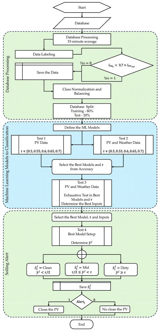
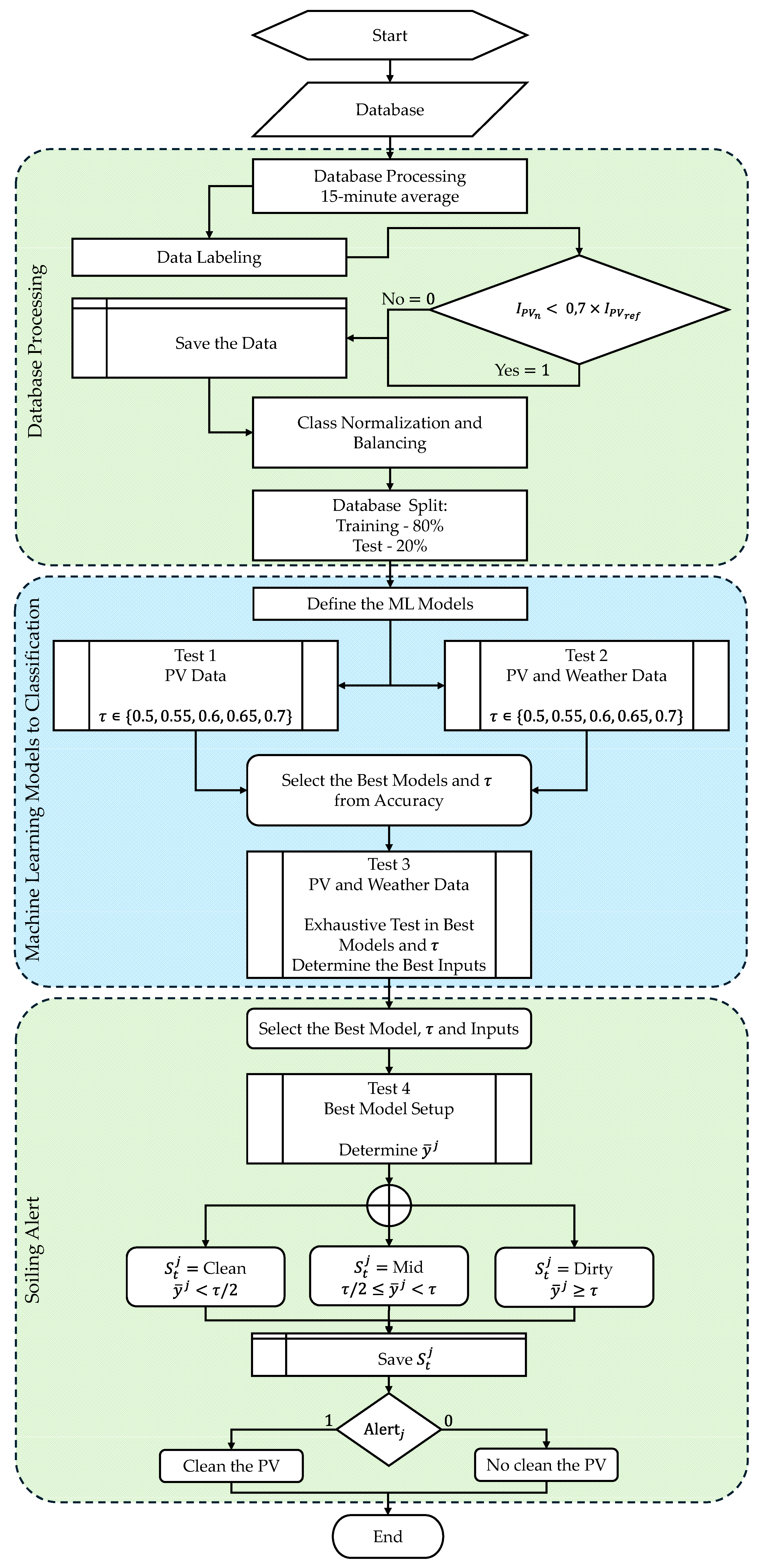
The methodology is structured and summarized in the general flowchart presented in Figure 1, which presents the main steps followed in the work.
Figure 1.
General flowchart of the framework used for determining the PV soiling status and the alert system.
Initially, experimental data from PV systems and a meteorological station were processed, including pre-processing, sample labeling, and a dataset structure for model training and testing. Next, different ML models were developed and evaluated for classifying the soiling status of PV panels, considering different input attribute arrangements and variations in the decision threshold. Finally, based on the model and configuration with the best performance, a strategy was implemented to determine the soiling status of the panels and define an alert criterion for cleaning, resulting in a scalable and adaptable structure applicable to different PV systems and operational scenarios, with the potential to support predictive maintenance strategies and energy performance optimization.
2.1. Dataset Processing
The test system for this study consists of four PV panels, with measurements taken on each panel individually. Of these panels, two were subjected to artificial pollution tests (PV1 and PV2), with controlled dirt application throughout the evaluation period. A third panel (PV3) was cleaned daily and used as a reference for ideal performance. Finally, the fourth panel (PV4) remained exposed to environmental conditions, accumulating dirt naturally over time.
The original database has a temporal resolution of 1 min and covers a period of 7 months, as presented in the Supplementary Materials. For analysis purposes, the data were reprocessed by aggregating the mean in 15 min intervals. Thus, each new point represents the mean of the values recorded in each 15 min interval. Subsequently, the dataset annotation for training the classification models was based on a comparative reference methodology, using the clean control panel, the PV3, as the standard. This approach was necessary because there were no prior manual annotations of the PV panels’ dirtiness. The central labeling criterion established that a sample is considered a dirty panel (labeled as “1”) when its current () shows a significant drop compared to the reference panel (), and all other samples are labeled as clean panels (labeled as “0”).
The labeling threshold was set at 70% of the current generated by the clean panel, a criterion applied exclusively during the period of greatest energy generation potential, which was between 10:00 AM and 3:00 PM. This definition was supported by preliminary analyses in which different labeling rules were tested, including thresholds of 70%, 80%, and 90%, as well as alternative criteria based on both current and power. This procedure was motivated by the fact that the choice of threshold can directly influence class assignment and, therefore, alter the balance between classification errors and the resulting performance metrics, as discussed in [37] on classifier thresholding and F1-oriented decision rules, although our study was based on accuracy. Among the evaluated options, the current-based rule with a 70% threshold yielded the best classification accuracy and was therefore selected. Furthermore, the 10:00 AM to 3:00 PM window was selected to ensure that comparisons were performed under adequate solar irradiance conditions, minimizing false positives that could occur during periods of low insolation. This restriction also means that samples outside this interval were excluded from the labeling procedure. Although suitable for the evaluated conditions, this choice may introduce sensitivity to site-specific and seasonal irradiance patterns, which should be considered when extending the approach to other operating scenarios. Finally, the labeling was implemented using conditional operations that simultaneously compared each panel’s measurement time and relative performance against the reference.
The data from the four PVs were consolidated into a single set, where each record was standardized with the same variables for each PV module, which contained the following data:
- Voltage—Voltage (V);
- Current—Current (A);
- Temperature—Temperature (°C);
- Power—Calculate power (W).
Additionally, data from a meteorological station is available, with the following measurements:
- GHI1 and GHI2—Solar irradiation (W/m2);
- DEW—Dew-point (°C);
- TEMP—Ambient temperature (°C);
- HUM—Relative humidity (%);
- SPEED—Wind speed (m/s).
To avoid problems with magnitude, the dataset was standardized using the normal distribution (), as expressed in Equation (1):
where is the real sample at time , is the mean of the samples, and is the standard deviation of the samples.
Subsequently, class balancing was performed using the Random Under-Sampling technique to equalize the representation of the “clean” and “dirty” classes, ensuring that the ML models did not exhibit bias towards the majority class. This strategy was adopted due to its simplicity and because it preserves only real observations from the dataset, without introducing synthetic samples. However, alternative approaches to class balancing may also be suitable. Finally, the dataset was divided into 80% for training and 20% for testing.
2.2. Classification Models Evaluation
The analysis involved developing ML models to classify operational data, with an emphasis on identifying PV module soiling status. Performance tests were conducted, encompassing the evaluation of different models, multiple arrangements of input variables, and distinct thresholds, given by . This process aimed to investigate the impact of attribute choices, labeling strategy, and decision limits on the predictive capacity of the classifiers, enabling the identification of the most efficient and robust models and configurations for the problem under study.
For the analyses, different ML models applied to classification were evaluated. The models tested included Bagging (BG), Decision Tree (DT), Extra Trees (ET), Gaussian Naive Bayes (GNB), Gradient Boosted Classifier (GBC), Histogram-based Gradient Boosting (HGB), K-Nearest Neighbors (KNNs), Multi-Layer Perceptron (MLP), Random Forest (RF), Stochastic Gradient Descent (SGD), Support Vector Classifier (SVC), and Extreme Gradient Boosting (XGB).
It is noteworthy that the default settings of the classification models were used. This choice was made to ensure methodological consistency and reproducibility across all evaluated models, while also avoiding model-specific tuning advantages that could favor some classifiers over others in the comparative analysis. From this, tests were conducted considering variations in of 0.5, 0.55, 0.6, 0.65, and 0.7. For example, during the training and testing steps of the models, for a of 0.5, predicted values ≥ 0.5 are classified as dirty panels, and predicted values < 0.5 are classified as clean panels, with the same logic applied to the different variations in . Two tests were then conducted: the first considered only the PV data, and the second included meteorological station data in addition to the PV data. Based on the test results, the models with the best accuracy were identified.
Next, an exhaustive test was conducted on the four models with the highest average accuracy. In this procedure, the models were evaluated considering all possible combinations of input features, with the aim of identifying, for each model and for each value, the attributes most representative of the database that resulted in the best accuracies. For cases in which the models yielded the same accuracy value, the lowest value was selected. This choice is because the lowest value is a less aggressive cutoff point for determining the soiling status of the PVs. Then, based on the models and configurations selected in this step, predictive performance was evaluated using the training and testing processing times and the classification metrics adopted in this study.
The classification problem adopted in this study was binary, with zero (“0”) representing a clean panel and one (“1”) representing a dirty panel. The models’ performance was evaluated using the confusion matrix. In this context, true positives (TP) corresponded to samples from the positive class correctly classified by the model, while true negatives (TN) corresponded to samples from the negative class correctly classified. False positives (FP) referred to samples from the negative class that were incorrectly classified as positive, while false negatives (FN) corresponded to samples from the positive class that were incorrectly classified as negative. During this stage, accuracy, precision, recall, and F1-score metrics were evaluated, along with the area under the receiver operating characteristic curve (AUC-ROC) analysis, as per the study by [38].
Accuracy was used to quantify the proportion of correct predictions made by the model relative to the total number of samples and is defined by Equation (2):
The precision assessed the reliability of the model’s positive and negative predictions, defined as the proportion of correctly classified samples among all predicted samples, as expressed in Equation (3):
The recall, also called sensitivity, measured the model’s ability to correctly identify samples belonging to the positive and negative classes, and it is defined by Equation (4):
The F1-score was used as a balanced metric between precision and recall, corresponding to the harmonic mean of these metrics. Its formulation is presented in Equation (5):
The Receiver Operating Characteristic (ROC) curve was constructed from the variation in the classifier’s decision , relating the true positive rate (TPR) and the false positive rate (FPR), defined by Equations (6) and (7), respectively:
Finally, the AUC-ROC was used as a global performance metric to evaluate the models’ discriminative capacity. AUC-ROC values close to 1 indicated a high capacity for separating classes, while values close to 0.5 indicated performance equivalent to random classification. With this, it was possible to determine the classification model and the best arrangement for the problem of identifying the state of soiling in PV panels.
2.3. Determination of the State of Soiling and the Alert System
After identifying the model and configuration with the best performance, the soiling status of the PVs was evaluated. During this test, the soiling status was assessed at three levels, namely clean, medium, and dirty, resulting in a cleaning alert strategy for the panels. The strategy adopted to communicate that the PVs were clean was based on daily analysis of floating windows over the last 7 days, using results from the classification model and its best configuration. For this, based on the daily result of the classification probabilities (), for each PV panel , with a time resolution of 15 min in the interval from 10:00 AM to 03:00 PM, the daily average () of this period was calculated according to Equation (8). From this, the direction of Equation (9) was used to determine the soiling status () of each PV panel:
where denotes the total number of samples considered in the analysis interval, represents the probability of soiling predicted by the model at time for PV panel , corresponds to the daily average of these probabilities for panel , and is the decision threshold used to discriminate daily as clean, mid, or dirty. It should be noted that the original model was trained as a binary classifier, with labels limited to clean and dirty. The mid status was introduced afterward as a post hoc interpretation of the probability outputs, by subdividing the clean side of the decision range to indicate proximity to the dirty condition, while preserving the original dirty threshold.
Next, based on the results of , an alert criterion was defined for cleaning each PV module individually, as expressed in Equation (10), in which the alert is triggered when
where equals 1 indicates that PV panel requires cleaning, and equals 0 indicates that no cleaning action is necessary. Furthermore, and represent, respectively, the relative frequencies of the mid and dirty classes for each PV panel , calculated from the daily distribution of dirt states . In turn, represents the classified dirt state for PV panel on the -th day prior to time . It should be noted that the terms and are defined as the ratio between the number of samples classified in each state and the total number of samples in the analyzed period. The criterion adopts two decision mechanisms defined empirically based on a series of fit tests: (i) a combined condition, in which the proportions of the mid and dirty classes must simultaneously exceed 30%, and (ii) a dominant condition, in which the dirty class must exceed 50% of the samples. Furthermore, an operational criterion was incorporated that suppresses the alert if at least one of the last three days is classified as clean, aiming to reduce false positives in maintenance decision-making.
These parameters were defined empirically as operational decision criteria rather than through formal optimization. From an O&M perspective, such criteria represent a trade-off between FP, which may lead to unnecessary cleaning actions, and FN, which may delay intervention and increase energy losses. Therefore, although effective under the evaluated conditions, these parameters may be adapted to different operational scenarios and maintenance priorities.
3. Results and Discussion
This section presents and discusses the results obtained from four evaluation stages. First, all ML models were trained and evaluated using only the PV module database, with threshold values ranging from 0.5 to 0.7. Subsequently, the same procedure was repeated with the complete database, incorporating weather features, to quantify the effect of environmental information on the classifiers’ performance. From these results, the four models with the highest average accuracy were selected. Next, an exhaustive search for attribute combinations was performed for these four models, again under between 0.5 and 0.7, to identify the most representative configuration and the model with the best overall performance. Finally, the selected model and configuration were applied to determine the dirtiness status of the panels and to trigger cleaning alerts, translating the classification probabilities into an operational logic oriented towards predictive maintenance.
3.1. Evaluation of Models with Operational Features of PV Modules
This test aimed to evaluate the ability of ML models to identify the state of soiling using only the operational features available in the PV modules. The purpose of this test was to verify whether the electrical and thermal behavior of the modules (voltage, current, power, and temperature) provided sufficient information for classification, and to quantify the sensitivity of performance to the choice of . The results obtained for each model and for each value of are presented in Table 1.
Table 1.
Accuracy results for PV module data.
Overall, high performance was observed for the main classifiers, especially ensemble-based approaches and non-linear methods. HGB showed the highest average accuracy (0.9448) and low variation across thresholds (0.9440–0.9459), indicating classifier stability under changes in the cutoff point. Following this, KNN achieved an average of 0.9425, maintaining performance up to = 0.6, with a slight reduction at ≥ 0.65. The ET and BG models also remained among the best, with averages of 0.9413 and 0.9409, respectively.
Although RF showed high maximum values (0.9459 at equal 0.5 and 0.55), it was more sensitive to increases in , dropping to 0.9324 at = 0.65, suggesting that the model was more affected by changes in the decision criterion when operating only with PV features. The GBC showed intermediate performance (mean 0.9386), while XGB exhibited the same result across the evaluated thresholds (mean 0.9324). Among the models with the lowest performance, DT maintained a constant mean of 0.9170, while MLP and SVC presented means of 0.9139 and 0.9124, respectively. Finally, SGD (mean 0.8853) and GNB (mean 0.8347) recorded the lowest accuracies, highlighting limitations in representing the soiling pattern based solely on operational features. From a physical point of view, this assessment was relevant because different loss mechanisms can produce similar electrical signatures, requiring robust models to avoid misinterpretations when surface effects and electrical faults overlap [9,10].
Given this, this evaluation demonstrated that the module data were sufficient to achieve high accuracies across several models but also indicated that performance and stability may vary with the classifier and threshold. Based on these findings, the next test investigated the potential gains from incorporating meteorological variables, evaluating whether additional weather information would improve the models’ performance.
3.2. Evaluation of the Models with the Complete Dataset
This analysis aimed to evaluate the impact of incorporating weather features on models’ ability to classify the state of soiling, considering both operational data from PV modules and meteorological station measurements. The objective was to verify whether information such as irradiance, humidity, ambient temperature, dew point, and wind would help reduce ambiguities associated with operational and environmental variability, and to analyze the stability of the models in the face of variations in the established value. The addition of weather features is aligned with data-driven approaches that integrate electrical quantities to improve detection and diagnosis in PV systems, as discussed in [20]. The results obtained for each model and for each value are presented in Table 2.
Table 2.
Accuracy results for PV module and weather data.
Based on the results in Table 2, a significant performance increase was observed compared to the scenario without weather data. The ET model showed the highest accuracy (0.9834), achieving its best values at = 0.55 and = 0.6 (0.9865). The HGB showed equally high performance and, above all, the most stable behavior among the evaluated thresholds, maintaining 0.9826 at all values (average 0.9826). Next, XGB obtained an average of 0.9768, with little oscillation and a maximum at = 0.6 (0.9788). RF reached an average of 0.9730, however, with greater sensitivity to the increase in the threshold, reducing from 0.9768 ( = 0.5) to 0.9653 ( = 0.7).
In the intermediate range, BG averaged 0.9707, with improvement at higher thresholds (up to 0.9730 at = 0.65–0.7). GBC and MLP maintained similar performance (averages of 0.9687 and 0.9676, respectively), with good predictive capacity when incorporating weather features. The methods such as KNN, SGD, and SVC showed lower average performance (0.9537, 0.9490, and 0.9444), while DT remained stable at 0.9363, and GNB registered the lowest performance (average 0.8699), though with a slight improvement at higher .
Regarding the first evaluation, the inclusion of weather features increased the overall average accuracy of the models from 0.9204 to 0.9563 (+3.59 p.p.) and increased the best absolute performance from 0.9459 to 0.9865 (+4.06 p.p.). This performance improvement aligns with the recent literature, which indicates greater model robustness when weather data are considered alongside PV module data, especially in scenarios of operational variability and the need for continuous monitoring [29,32]. Therefore, based on the average accuracies of the complete dataset, the four models with the best performance were selected for the next stage: ET, HGB, XGB, and RF. From this selection, an exhaustive test was performed for these models, evaluating combinations of attributes and values, with the aim of determining the most representative configuration and the best overall model for operational application.
3.3. Exhaustive Testing on Selected Models
The purpose of this step was to verify whether the previously observed selection held when the models were analyzed more thoroughly and, primarily, to select a model with stable performance relative to other metrics in the face of variations in . Furthermore, as described in the methodology, the choice of considered the tie-breaking rule of the lowest value, as it represents a less aggressive threshold in identifying dirtiness. It was observed that the four models exhibited high performance across the evaluated metrics, as shown in Table 3.
Table 3.
Best results for the exhaustive test.
Observing the results in Table 3, it was found that the four models presented high overall performance, with accuracies above 0.98, AUC-ROC scores above 0.99, and high F1-scores in both classes, indicating a robust classification between clean (0) and dirty (1). Although the differences were small, ET ( = 0.5) stood out for combining the highest accuracy (0.9884) and the highest AUC-ROC (0.9957), in addition to presenting high precision and recall in both classes: for class 0, precision of 0.9962 and recall of 0.9811 (F1 = 0.9886), and for class 1, precision of 0.9805 and recall of 0.9960 (F1 = 0.9882). The HIST ( = 0.55) showed very similar performance and well-balanced metrics, while XGB ( = 0.5) and RF ( = 0.6) remained competitive, with accuracy and recall metrics comparable to ET and HIST, but slightly lower.
Considering the behavior by class, ET showed very high recall for class 1 (0.9960), a desirable characteristic to reduce the chance of classifying dirty panels as clean (false negatives), while maintaining high precision and F1-score. Additionally, the HIST model also maintained a balance between precision and recall in both classes, suggesting similar robustness. From a computational point of view, processing times were very similar across the models (≈6 s), indicating that the choice of classifier could prioritize performance and stability without a significant execution penalty in this study.
Moreover, Table 4 complemented this analysis by highlighting which features contributed to the best performance of each model in the selected configuration. It was observed that GHI1 and GHI2 were selected in all the best configurations (HIST, XGB, ET, and RF), indicating that irradiance information was central to explaining performance variations and supporting the discrimination between classes, since it helps distinguish reduced PV output caused by low solar resource from losses associated with soiling. The Temperature and Voltage were also present in all cases, indicating that, in addition to the environmental context provided by irradiance, the thermal and electrical behavior of the PV module also played a relevant role in class discrimination. Additionally, the feature Temperature affects the electrical response of the PV module, while Voltage reflects changes in operating conditions associated with the PV module performance. In the context of soiling, this is particularly important because surface deposition reduces the effective irradiance reaching the cells, which can alter the electrical operating point and contribute to differences in voltage behavior under comparable weather conditions.
Table 4.
Features for the best arrangements of each model.
Furthermore, there were differences between models: HIST was the only one to select additional weather features (DEW and TEMP) combined with Power; XGB and RF incorporated SPEED and Current, while ET combined irradiance with Power. Wind may influence both dust deposition and partial natural cleaning, affecting soiling persistence over time. Taken together, these results indicated that, although irradiance and temperature were common features, each model prioritized distinct subsets to maximize accuracy.
The processing times reported in Table 4 correspond to the best configuration selected for each model, relative to the respective decision thresholds shown in the table. It should be noted, however, that the exhaustive analyses were performed for five threshold values (0.5, 0.55, 0.6, 0.65, and 0.7). Across these threshold variations, the observed processing times remained close to the presented values, indicating no substantial computational deviation among the evaluated cutoff values.
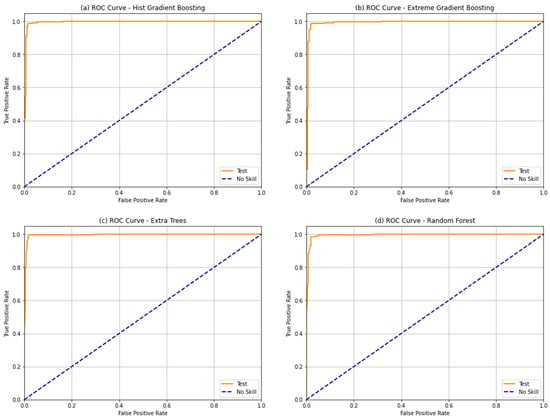
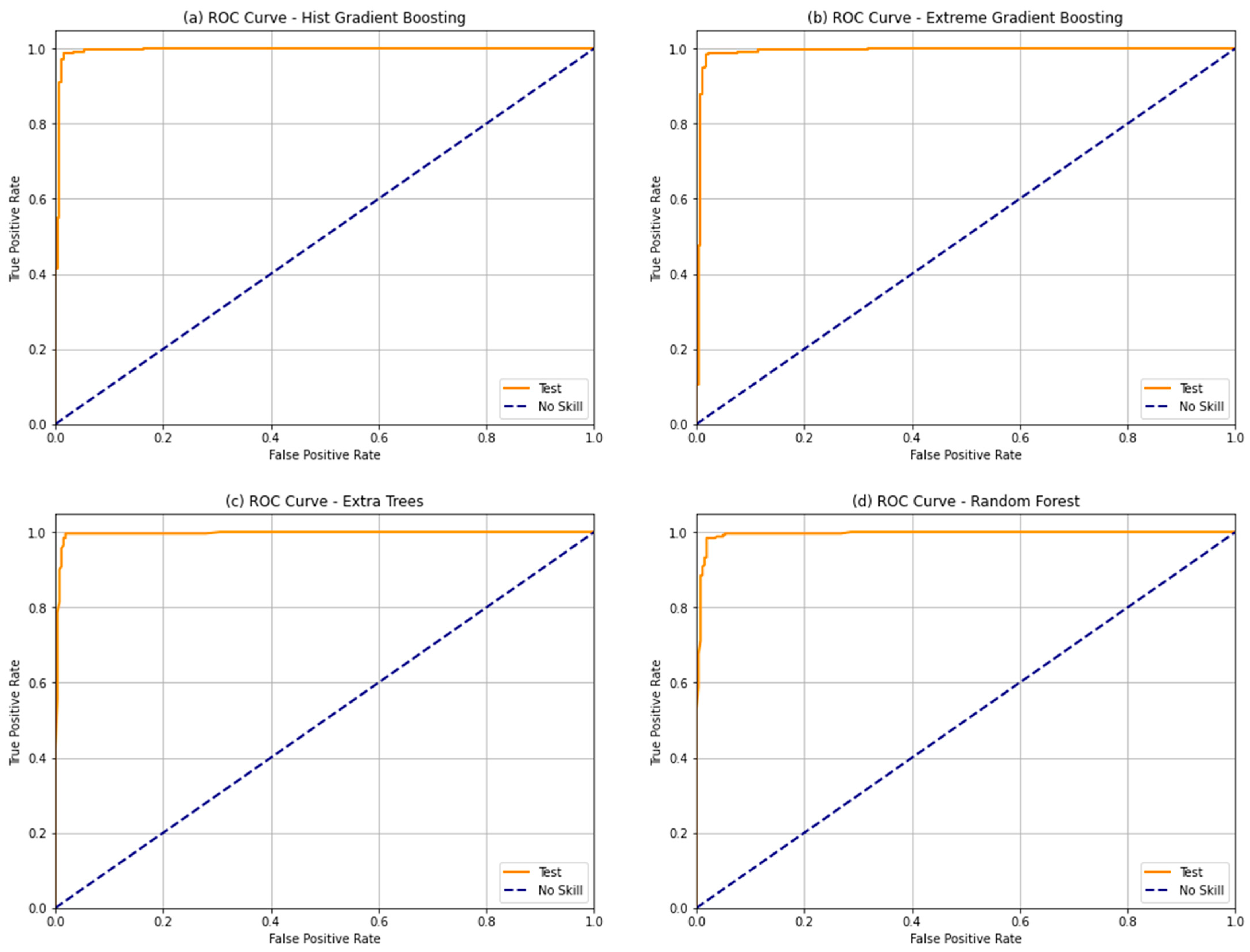
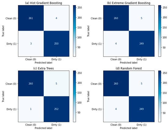
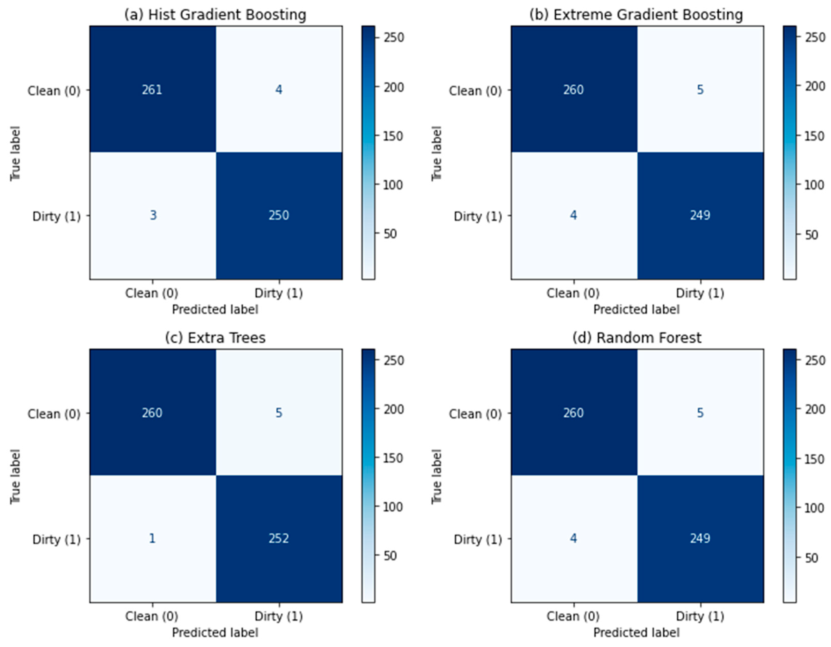
In addition, the ROC curves and confusion matrices for the four models are presented in a single block in Figure 2 and Figure 3, respectively. It was observed that the ROC curves remained concentrated near the upper left corner for all models, indicating high discriminative capacity with the AUC-ROC values reported in Table 3. In practical terms, the confusion matrices showed that the four classifiers made few errors, with a predominance of correct classifications in both classes. The ET model presented the lowest total incidence of errors, with 5 FP and only 1 FN. The HIST model showed very similar performance, with 4 FP and 3 FNs, while RF and XGB showed equivalent patterns, with 5 FP and 4 FN.
Figure 2.
ROC Curves: (a) Histogram-based Gradient Boosting; (b) Extreme Gradient Boosting; (c) Extra Trees; (d) Random Forest.
Figure 3.
Confusion Matrices: (a) Histogram-based Gradient Boosting; (b) Extreme Gradient Boosting; (c) Extra Trees; (d) Random Forest.
From an operational perspective, FP may result in unnecessary cleaning recommendations, while FN may delay intervention in soiled panels. These misclassifications may be related to short-term weather variability, measurement noise, and partial overlap between weather effects and soiling-related electrical behavior, which can reduce class separability in specific samples. These results also do not suggest evident overfitting, as the models consistently achieved high and balanced accuracy, precision, recall, F1-score, and AUC-ROC, as shown in Table 3. The low number of errors is therefore coherent with the overall robustness of the selected classifiers under the evaluated test conditions.
Finally, these results reinforced the idea that all four models are viable from a predictive standpoint. However, the ET model presented the best overall performance and, among classes, was therefore chosen for the subsequent operational stage. Following this, the selected model was applied to determine the soiling status of the PV panels over time and to operationalize the cleaning alert criterion, translating the classification probabilities into levels (clean, mid, and dirty) and into a maintenance trigger rule.
3.4. Results of Determining the Soiling Status of the PV Panels and the Alert System
To assess the soiling status of the PV panels used in this study, a dataset was reserved, with a total of 12 days of sampling. In this step, the selected model was used to estimate the daily soiling status of each PV panel at three levels (clean, mid, and dirty), as defined by the criteria described in the methodological section. To facilitate visual interpretation of the results, the clean state was represented in green, the mid state in orange, and the dirty state in red. Based on this classification, the was calculated, with state 1 indicating the need for cleaning and state 0 indicating that no action was required, according to the established decision rule. It should be noted that panels PV1 and PV2 were subjected to soiling tests, while panels PV3 and PV4 remained with natural soiling accumulation. Thus, the results of this stage are presented in Table 5, Table 6, Table 7 and Table 8, corresponding to panels PV1, PV2, PV3, and PV4, respectively. For clarity, the values in Table 5, Table 6, Table 7 and Table 8 are displayed according to the rolling-window structure used in the alert logic. Thus, repeated entries do not indicate duplicate data, but rather the same daily probability within successive moving windows used to evaluate the persistence of soiling over time.
Table 5.
Estimated average daily probability and soiling status of PV1 in the test set.
Table 6.
Estimated average daily probability and soiling status of PV2 in the test set.
Table 7.
Estimated average daily probability and soiling status of PV3 in the test set.
Table 8.
Estimated average daily probability and soiling status of PV4 in the test set.
For PV1, the daily classification indicated a predominance of mid and dirty states for most of the initial period, with high average daily probabilities, which resulted in the activation of the alert in the moving windows corresponding to days 7, 8, and 9. It should be noted that, at this stage, controlled tests were conducted by applying dirt on consecutive days to evaluate the model’s ability to maintain the signaling of the need for cleaning under the persistence of the soiling. From day 10 onwards, a sharp reduction in probability (21.90%) was observed, classified as clean, followed by intermediate values, which led to the alert ceasing from that point.
Similarly, in PV2, the behavior showed a more gradual transition, with initial values predominantly in the mid-range, followed by a period with higher probabilities, which increased the dirty class index in the moving windows and allowed the alert criterion to be met. As a result, was not triggered at the first decision point (day 7) but was triggered in two consecutive evaluations, i.e., in the windows closed on days 8 and 9, indicating persistent dirtiness at a level sufficient to satisfy the established conditions. From day 10 onwards, a significant drop in probabilities was observed (≈19.76%, classified as clean), followed by intermediate values, which resulted in the cessation of the alert because there was at least one clean state among the last three days, with remaining at 0 on days 10, 11 and 12, in accordance with the adopted rule, as was the case for PV1.
For PV3 and PV4, no forced or controlled dirt application was performed, and both panels remained exposed to natural environmental conditions. Therefore, the observed variation in the estimated probabilities reflected natural operating and environmental conditions, including natural soiling effects, rather than controlled soiling accumulation. In this context, the application of the alert criterion with a 7-day rolling window was useful to avoid false triggers due to isolated events, since the alert depends on the persistence of mid/dirty states throughout the window or the dominance of dirty states, in addition to the operational criterion associated with the operating state of the last few days. Thus, for PV3 and PV4, the observed behavior reflected natural field conditions, with no persistent soiling pattern strong enough to satisfy the alert criterion throughout the evaluated period. Consequently, no cleaning alert was triggered for these panels.
Finally, the alert system responded consistently to the evaluated scenarios. In the PV panels subjected to controlled tests, the alert was triggered when mid/dirty states persisted and ceased after the estimated levels decreased. Under natural environmental conditions, there was no significant dirt on the PV panels, as evidenced by the estimated relative probabilities, resulting in no triggering. Thus, the approach demonstrated the potential to support O&M decisions in an objective and scalable way, reducing false alerts and prioritizing interventions when dirt accumulation remained significant over time.
4. Conclusions
Soiling in PV modules is a recurring challenge in different regions and operating conditions, as it reduces energy performance and requires efficient O&M decisions to determine when to intervene with cleaning. This study proposed and evaluated an ML-based approach to identify the state of soiling on PV panels and to trigger cleaning alerts from operational and weather data. In tests using features exclusively from the PV modules, the models achieved high performance, with average accuracies ranging from 0.83 to 0.94, showing that electrical and thermal signals are essential for the classification. However, the inclusion of weather features yielded performance gains, increasing the overall average accuracy of the models and improving the best absolute performance, indicating higher discrimination capacity when the environmental context was considered.
The exhaustive analysis of feature and threshold combinations confirmed the robust performance of the four finalist models and enabled the selection of the better model and configuration for operational use. The ET model, with = 0.5, presented the best combination of performance and between classes, with accuracy = 0.9884, AUC-ROC = 0.9957, and high values across the other metrics, in addition to a low incidence of errors, while maintaining a processing time of 6 s, compatible with practical application. Finally, the strategy for determining the daily state (clean, mid, and dirty) and the alert criterion based on a moving window responded consistently to the evaluated scenarios, triggering alerts under persistent controlled soiling conditions and remaining inactive when natural conditions did not sustain a soiling pattern sufficient to meet the alert criterion. In addition, for the PV panels subjected to controlled tests, the alert was triggered due to the persistence of dirt and ceased after the reduction in the estimated levels, whereas in the PV panels under natural environmental conditions, no temporal windows met the alert criterion, resulting in no trigger. Taken together, the results highlight the approach’s potential to support O&M decisions in an objective, scalable, and predictive manner, reducing false alerts and prioritizing interventions when soiling accumulation remained significant over time.
In conclusion, as future work, it is recommended to expand the validation set across different climatic and seasonal periods and to investigate strategies for calibrating the decision threshold for different configurations in large PV power plants. Additionally, it is proposed to evaluate the embedding of the model in hardware for operation in Edge AI, enabling local real-time inference with low latency and greater system autonomy, in addition to integrating the method into supervisory environments with continuous monitoring and periodic model updates.
Supplementary Materials
The following supporting information can be downloaded at https://www.mdpi.com/article/10.3390/en19081964/s1.
Author Contributions
Conceptualization, B.K.H., J.C.J.J. and L.M.; methodology, B.K.H., J.C.J.J., L.M., E.A.T. and N.P.M.; software, B.K.H., J.C.J.J. and L.M.; validation, B.K.H., J.C.J.J., L.M., P.H.d.F. and R.M.S.; formal analysis, E.A.T., P.H.d.F. and N.P.M.; investigation, B.K.H., J.C.J.J. and E.A.T.; resources, R.M.S. and N.P.M.; data curation, B.K.H., L.M. and P.H.d.F.; writing—original draft preparation, B.K.H., J.C.J.J. and E.A.T.; writing—review and editing, E.A.T., P.H.d.F. and R.M.S.; visualization, N.P.M.; supervision, R.M.S. and N.P.M.; project administration, R.M.S. and N.P.M.; funding acquisition, R.M.S. and N.P.M. All authors have read and agreed to the published version of the manuscript.
Funding
This work has been fully funded by the project SOLO—Desenvolvimento de métodos de machine learning embarcados para identificação de queda de performance em sistemas fotovoltaicos por sujidade supported by Future Grid—Centro e Competência Embrapii Lactec em Smart Grid e Eletromobilidade, with financial resources from the PPI HardwareBR of the MCTI grant number 054/2023, signed with EMBRAPII.
Data Availability Statement
The data presented in this study might be available on request from the corresponding author.
Conflicts of Interest
Authors B.K.H., J.C.J.J., L.M., E.A.T., P.H.F., R.M.S., and N.P.M. were employed by the company Future Grid. The remaining authors declare that the research was conducted in the absence of any commercial or financial relationships that could be construed as a potential conflict of interest.
Abbreviations
The following abbreviations are used in this manuscript:
| O&M | Operation and Maintenance |
| PV | Photovoltaic |
| ML | Machine Learning |
| AI | Artificial Intelligence |
| DL | Deep Learning |
| YOLO | You Only Look Once |
| CNN | Convolutional Neural Network |
| RNN | Recurrent Neural Network |
| GNN | Graph Neural Network |
| IoT | Internet of Things |
| AIoT | Artificial Intelligence of Things |
| BG | Bagging |
| DT | Decision Tree |
| ET | Extra Trees |
| GNB | Gaussian Naive Bayes |
| GBC | Gradient Boosted Classifier |
| HGB | Histogram-based Gradient Boosting |
| KNN | K-Nearest Neighbors |
| MLP | Multi-Layer Perceptron |
| SGD | Stochastic Gradient Descent |
| SVC | Support Vector Classifier |
| XGB | Extreme Gradient Boosting |
| TP | True Positives |
| TN | True Negatives |
| FP | False Positives |
| FN | False Negatives |
| AUC-ROC | Area Under the Receiver Operating Characteristic Curve |
| ROC | Receiver Operating Characteristic |
| TPR | True Positive Rate |
| FPR | False Positive Rate |
References
- Sharma, S.; Raina, G.; Yadav, S.; Sinha, S. A Comparative Evaluation of Different PV Soiling Estimation Models Using Experimental Investigations. Energy Sustain. Dev. 2023, 73, 280–291. [Google Scholar] [CrossRef] [Scilit]
- Tonolo, É.A.; Mariano, J.D.A.; Urbanetz Junior, J. Análise do Efeito do Acúmulo de Sujeira nos Sistemas Fotovoltaicos da UTFPR—Câmpus Curitiba. Available online: https://anaiscbens.emnuvens.com.br/cbens/article/view/183/183 (accessed on 10 March 2026).
- Al-Humairi, A.; Khalis, E.; Al-Hemyari, Z.A.; Jung, P. Machine Learning-Based Predictive Maintenance for Photovoltaic Systems. AI 2025, 6, 133. [Google Scholar] [CrossRef] [Scilit]
- Triki-Lahiani, A.; Bennani-Ben Abdelghani, A.; Slama-Belkhodja, I. Fault Detection and Monitoring Systems for Photovoltaic Installations: A Review. Renew. Sustain. Energy Rev. 2018, 82, 2680–2692. [Google Scholar] [CrossRef] [Scilit]
- Yang, R.L.; Máximo Tiepolo, G.; Tonolo, É.A.; Junior, J.U.; Bester De Souza, M. Estimação da Temperatura em Células Fotovoltaicas para Sistemas Fotovoltaicos Conectados à Rede Elétrica em Curitiba. Available online: https://utfpr-ct-static-content.s3.amazonaws.com/utfpr.curitiba.br/wp-content/uploads/sites/85/2018/11/Estimacao_da_temperatura_em_celulas_fotovoltaicas_para_sistemas_fotovoltaicos_conectados_a_rede_eletrica_em_Curitiba_VF.pdf (accessed on 10 March 2026).
- Hammerschmitt, B.K.; Rambo, M.V.H.; Leone, A.d.S.; Iantorno, L.M.; Schiavon, H.B.; Corrêa, D.P.; Lissa, P.; Keane, M.; Riella, R.J. Deep Learning for Residential Electrical Energy Consumption Forecasting: A Hybrid Framework with Multiscale Temporal Analysis and Weather Integration. Energies 2025, 18, 5885. [Google Scholar] [CrossRef] [Scilit]
- Suliman, F.; Anayi, F.; Packianather, M. Electrical Faults Analysis and Detection in Photovoltaic Arrays Based on Machine Learning Classifiers. Sustainability 2024, 16, 1102. [Google Scholar] [CrossRef] [Scilit]
- Madeti, S.R.; Singh, S.N. Monitoring System for Photovoltaic Plants: A Review. Renew. Sustain. Energy Rev. 2017, 67, 1180–1207. [Google Scholar] [CrossRef] [Scilit]
- Spataru, S.; Sera, D.; Kerekes, T.; Teodorescu, R. Diagnostic Method for Photovoltaic Systems Based on Light I–V Measurements. Sol. Energy 2015, 119, 29–44. [Google Scholar] [CrossRef] [Scilit]
- Qu, J.; Sun, Q.; Qian, Z.; Wei, L.; Zareipour, H. Fault Diagnosis for PV Arrays Considering Dust Impact Based on Transformed Graphical Features of Characteristic Curves and Convolutional Neural Network with CBAM Modules. Appl. Energy 2024, 355, 122252. [Google Scholar] [CrossRef] [Scilit]
- Eshwaran Ramachandran, M.; Babu Balachandran, G.; Velladurai, P.; Rajakumar, A. Deep Learning for Solar PV Fault Classification Using RGB Imaging and Comparison of Preprocessing Techniques. Sol. Energy 2025, 301, 113959. [Google Scholar] [CrossRef] [Scilit]
- Ebied, M.A.; Munshi, A.; Alhuzali, S.A.; El-sotouhy, M.M.; Shehta, A.I.; Elborlsy, M.S. Advanced Deep Learning Modeling to Enhance Detection of Defective Photovoltaic Cells in Electroluminescence Images. Sci. Rep. 2025, 15, 31640. [Google Scholar] [CrossRef] [Scilit] [PubMed]
- Ayunts, H.; Agaian, S.S.; Grigoryan, A.M. Solar Photovoltaic System Fault Classification via Hierarchical Deep Learning with Imbalanced Multi-Class Thermal Dataset. Energies 2026, 19, 462. [Google Scholar] [CrossRef] [Scilit]
- Teta, A.; Korich, B.; Bakria, D.; Hadroug, N.; Rabehi, A.; Alsharef, M.; Bajaj, M.; Zaitsev, I.; Ghoneim, S.S.M. Fault Detection and Diagnosis of Grid-Connected Photovoltaic Systems Using Energy Valley Optimizer Based Lightweight CNN and Wavelet Transform. Sci. Rep. 2024, 14, 18907. [Google Scholar] [CrossRef] [Scilit]
- Hamid, A.-K.; Alrahhal, M.; Obaideen, K.; Bonny, T.; Tan, Y.C.; Hussein, M.I. Artificial Intelligence for Smart Solar Energy Monitoring: Genetic Attention-Based Hybrid Deep–Handcrafted Fusion for Faulty Solar Panel Image Classification. Results Eng. 2025, 28, 107900. [Google Scholar] [CrossRef] [Scilit]
- Guo, Y.; Wang, X.; Lin, Z. RFE-YOLO: A Study on Photovoltaic Module Fault Detection Algorithm Based on Multimodal Feature Fusion. Sensors 2025, 25, 6774. [Google Scholar] [CrossRef] [Scilit]
- Onim, M.S.H.; Sakif, Z.M.M.; Ahnaf, A.; Kabir, A.; Azad, A.K.; Oo, A.M.T.; Afreen, R.; Hridy, S.T.; Hossain, M.; Jabid, T.; et al. SolNet: A Convolutional Neural Network for Detecting Dust on Solar Panels. Energies 2022, 16, 155. [Google Scholar] [CrossRef] [Scilit]
- Bassil, J.; Noura, H.N.; Salman, O.; Chahine, K.; Guizani, M. Efficient Combination of Deep Learning and Tree-Based Classification Models for Solar Panel Dust Detection. Intell. Syst. Appl. 2025, 26, 200509. [Google Scholar] [CrossRef] [Scilit]
- El Karch, H.; El Gouri, R.; Natij, Y.; Benally, M.; Mezouari, A. AI-Based Smart Real-Time PV Panels Soiling Recognizing System Using Deep Neural Network Framework on NVIDIA Jetson Nano Embedded GPU. Int. Inf. Eng. Technol. Assoc. 2024, 29, 1687–1699. [Google Scholar] [CrossRef] [Scilit]
- Lu, X.; Lin, P.; Cheng, S.; Fang, G.; He, X.; Chen, Z.; Wu, L. Fault Diagnosis Model for Photovoltaic Array Using a Dual-Channels Convolutional Neural Network with a Feature Selection Structure. Energy Convers. Manag. 2021, 248, 114777. [Google Scholar] [CrossRef] [Scilit]
- Tchoketch Kebir, S.; Cheggaga, N.; Ilinca, A.; Boulouma, S. An Efficient Neural Network-Based Method for Diagnosing Faults of PV Array. Sustainability 2021, 13, 6194. [Google Scholar] [CrossRef] [Scilit]
- Klinsuwan, T.; Ratiphaphongthon, W.; Wangkeeree, R.; Wangkeeree, R.; Sirisamphanwong, C. Evaluation of Machine Learning Algorithms for Supervised Anomaly Detection and Comparison between Static and Dynamic Thresholds in Photovoltaic Systems. Energies 2023, 16, 1947. [Google Scholar] [CrossRef] [Scilit]
- Ratsheola, K.; Setlhaolo, D.; Rasool, A.; Ali, A.; Mabunda, N.E. A Hybrid Artificial Intelligence for Fault Detection and Diagnosis of Photovoltaic Systems Using Autoencoders and Random Forests Classifiers. Eng 2025, 6, 254. [Google Scholar] [CrossRef] [Scilit]
- da Silveira Junior, C.R.; Sousa, C.E.R.; Fonseca Alves, R.H. Automatic Fault Classification in Photovoltaic Modules Using Denoising Diffusion Probabilistic Model, Generative Adversarial Networks, and Convolutional Neural Networks. Energies 2025, 18, 776. [Google Scholar] [CrossRef] [Scilit]
- Hueros-Barrios, P.J.; Rodríguez Sánchez, F.J.; Martín Sánchez, P.; Santos-Pérez, C.; Sangwongwanich, A.; Novak, M.; Blaabjerg, F. Digital Twin Approach for Fault Diagnosis in Photovoltaic Plant DC–DC Converters. Sensors 2025, 25, 4323. [Google Scholar] [CrossRef] [Scilit]
- Van Gompel, J.; Spina, D.; Develder, C. Satellite Based Fault Diagnosis of Photovoltaic Systems Using Recurrent Neural Networks. Appl. Energy 2022, 305, 117874. [Google Scholar] [CrossRef] [Scilit]
- Van Gompel, J.; Spina, D.; Develder, C. Cost-Effective Fault Diagnosis of Nearby Photovoltaic Systems Using Graph Neural Networks. Energy 2023, 266, 126444. [Google Scholar] [CrossRef] [Scilit]
- Liu, J.; Huang, Y.; Chen, K.; Liu, G.; Yan, J.; Chen, S.; Xie, Y.; Yu, Y.; Huang, T. Graph Neural Networks for Fault Diagnosis in Photovoltaic-Integrated Distribution Networks with Weak Features. Sensors 2025, 25, 5691. [Google Scholar] [CrossRef] [Scilit]
- Mellit, A.; Benghanem, M.; Kalogirou, S.; Massi Pavan, A. An Embedded System for Remote Monitoring and Fault Diagnosis of Photovoltaic Arrays Using Machine Learning and the Internet of Things. Renew. Energy 2023, 208, 399–408. [Google Scholar] [CrossRef] [Scilit]
- Sairam, S.; Seshadhri, S.; Marafioti, G.; Srinivasan, S.; Mathisen, G.; Bekiroglu, K. Edge-Based Explainable Fault Detection Systems for Photovoltaic Panels on Edge Nodes. Renew. Energy 2022, 185, 1425–1440. [Google Scholar] [CrossRef] [Scilit]
- Abdul-Rahaim, L.A.; Rahi, A.S. Intelligent Fault Detection Algorithm of PV System Based on Cloud Computing. Int. J. Electron. Commun. Eng. 2024, 11, 99–107. [Google Scholar] [CrossRef] [Scilit]
- Lodhi, E.; Liu, X.; Xiong, G.; Khan, M.A.; Lodhi, Z.; Nawaz, T.; Dilawar, A.; Tarkoma, S.; Wang, F. SmartPV-AIoT: An AIoT-Integrated Framework for Fault Diagnosis and Remote Monitoring in Photovoltaic Systems. Energy Convers. Manag. X 2025, 27, 101117. [Google Scholar] [CrossRef] [Scilit]
- Hojabri, M.; Kellerhals, S.; Upadhyay, G.; Bowler, B. IoT-Based PV Array Fault Detection and Classification Using Embedded Supervised Learning Methods. Energies 2022, 15, 2097. [Google Scholar] [CrossRef] [Scilit]
- Joshua, S.R.; Yeon, A.N.; Park, S.; Kwon, K. A Hybrid Machine Learning Approach: Analyzing Energy Potential and Designing Solar Fault Detection for an AIoT-Based Solar–Hydrogen System in a University Setting. Appl. Sci. 2024, 14, 8573. [Google Scholar] [CrossRef] [Scilit]
- Bougoffa, M.; Benmoussa, S.; Djeziri, M.; Palais, O. Hybrid Deep Learning for Fault Diagnosis in Photovoltaic Systems. Machines 2025, 13, 378. [Google Scholar] [CrossRef] [Scilit]
- Zgraggen, J.; Guo, Y.; Notaristefano, A.; Goren Huber, L. Physics Informed Deep Learning for Tracker Fault Detection in Photovoltaic Power Plants. In Proceedings of the 14th Annual Conference of the Prognostics and Health Management Society, Nashville, TN, USA, 1–4 November 2022; Volume 14. [Google Scholar] [CrossRef] [Scilit]
- Lipton, Z.C.; Elkan, C.; Naryanaswamy, B. Optimal Thresholding of Classifiers to Maximize F1 Measure. In Machine Learning and Knowledge Discovery in Databases; Calders, T., Esposito, F., Hüllermeier, E., Meo, R., Eds.; Lecture Notes in Computer Science; Springer Nature: Berlin/Heidelberg, Germany, 2014; pp. 225–239. [Google Scholar]
- Capeletti, M.B.; Hammerschmitt, B.K.; Negri, R.G.; Guarda, F.G.K.; Prade, L.R.; Knak Neto, N.; Abaide, A.d.R. Identification of Nontechnical Losses in Distribution Systems Adding Exogenous Data and Artificial Intelligence. Energies 2022, 15, 8794. [Google Scholar] [CrossRef] [Scilit]

Disclaimer/Publisher’s Note: The statements, opinions and data contained in all publications are solely those of the individual author(s) and contributor(s) and not of MDPI and/or the editor(s). MDPI and/or the editor(s) disclaim responsibility for any injury to people or property resulting from any ideas, methods, instructions or products referred to in the content. |
© 2026 by the authors. Licensee MDPI, Basel, Switzerland. This article is an open access article distributed under the terms and conditions of the Creative Commons Attribution (CC BY) license.