Transient Voltage Stability Assessment Method Based on CWT-ResNet

Abstract

Accurate and rapid transient voltage stability assessment is crucial for the safe and stable operation of new energy bases in desert and grassland regions. Existing deep learning methods fail to adequately capture the high-dimensional dynamic coupling features of transient voltage signals in large-scale renewable energy bases with UHVDC transmission, and suffer from poor performance under class-imbalanced sample conditions. This paper proposes a transient voltage stability assessment method utilizing continuous wavelet transform (CWT) time–frequency images and a deep residual network (ResNet-50). CWT with the Morlet wavelet basis converts voltage time-series signals into multi-scale time–frequency images to simultaneously capture temporal and frequency-domain transient features. An improved focal loss (FL) function is introduced to dynamically adjust category weights based on actual sample distribution, enhancing model robustness under extreme class imbalance. The proposed method is validated on a modified IEEE 39-bus system incorporating the Qishao UHVDC line and wind/photovoltaic integration in Northwest China, using 1490 simulation samples under diverse fault scenarios. Results demonstrate that the proposed CWT-ResNet achieves 98.88% accuracy, 94.74% precision, 100% recall, and 97.29% F1-score, outperforming SVM, 1D-CNN, and 1D-ResNet baselines. Under 5 dB noise conditions, the method maintains over 90% accuracy, demonstrating strong noise robustness.

1. Introduction

The rapid expansion of renewable energy generation and the widespread deployment of power electronic devices have fundamentally altered the dynamic characteristics of modern power systems, leading to heightened structural complexity and increasingly prominent voltage stability challenges [1]. In China, wind and solar resources are predominantly concentrated in desert, Gobi, and barren regions far from load centers; consequently, ultra-high voltage direct current (UHVDC) transmission has become indispensable for large-scale renewable energy integration [2,3]. At the DC sending ends of such renewable energy bases, the absence of conventional synchronous generation causes severe reactive power imbalances during fault events—such as commutation failures—thereby triggering transient voltage instability [4]. As renewable energy penetration continues to grow, the transient stability mechanisms at DC sending ends become increasingly complex [5], making transient voltage stability assessment (TVSA) more challenging and hindering power system planning and operational optimization. However, no deep learning-based TVSA method has been specifically designed for large-scale renewable energy bases in desert, Gobi, and wasteland regions with UHVDC transmission—the key gap that motivates this work.

Traditional TVSA methods include time-domain simulation [6] and energy function approaches [7,8]. Time-domain simulation provides accurate results but is computationally prohibitive for real-time applications [9,10], while energy function methods rely on simplifying assumptions that often yield overly conservative stability margins. With advances in artificial intelligence and wide-area measurement technology, data-driven approaches have emerged as effective alternatives that learn nonlinear input–output stability mappings without requiring detailed physical models [11,12]. Shallow machine learning algorithms—including decision trees (DTs) [13], support vector machines (SVMs) [14], and extreme learning machines (ELMs) [15]—have been applied to TVSA; however, these methods depend heavily on manual feature engineering, introducing subjectivity and limiting generalizability.

Deep learning models such as convolutional neural networks (CNNs), deep residual networks, and long short-term memory (LSTM) networks [16,17] overcome these limitations by automatically extracting hierarchical features from raw data. Recent advances in CNN-based TVSA include a Bayesian variational CNN ensemble [18] that extracts spatiotemporal grid features via parallel branches with variational inference fusion to reduce misclassification rates, and a residual CNN architecture [19] that mitigates gradient vanishing through skip connections. Despite these advances, two critical limitations remain. First, existing methods neglect channel-wise feature diversity and lack dynamic weight adjustment mechanisms, making fixed average feature aggregation inadequate for the high-dimensional dynamic coupling characteristics inherent to large-scale renewable bases. Second, transient stability datasets are inherently class-imbalanced. Data augmentation via conditional GANs [20] cannot guarantee physical fidelity of synthetic samples, and weighted cross-entropy [21] relies on empirical weight selection rather than adaptive adjustment—both failing to reliably handle extreme imbalance across multiple scenarios.

To address these challenges, this paper proposes a transient voltage stability assessment method integrating continuous wavelet transform (CWT) time–frequency images with a deep residual network (ResNet-50). Specifically, the main contributions are as follows: (1) CWT with the Morlet wavelet basis converts voltage time-series signals into multi-scale time–frequency images to simultaneously capture temporal and frequency-domain transient features, resolving the high-dimensional dynamic coupling challenge. (2) An improved focal loss (FL) function is introduced, incorporating a category–number balancing factor λ_i to dynamically adjust loss weights according to actual sample distribution, enhancing model robustness under extreme class imbalance. (3) The proposed method is the first deep learning approach specifically designed and validated for the “desert–grassland–wasteland” renewable energy base configuration with UHVDC transmission in Northwest China, using 1490 simulation samples under diverse fault scenarios on a modified IEEE 39-bus system.

2. Deep Residual Networks Based on Continuous Wavelet Transform

2.1. Deep Residual Network Model with Continuous Wavelet Transform

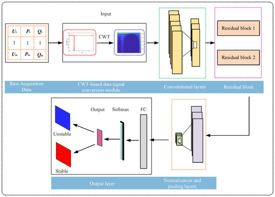
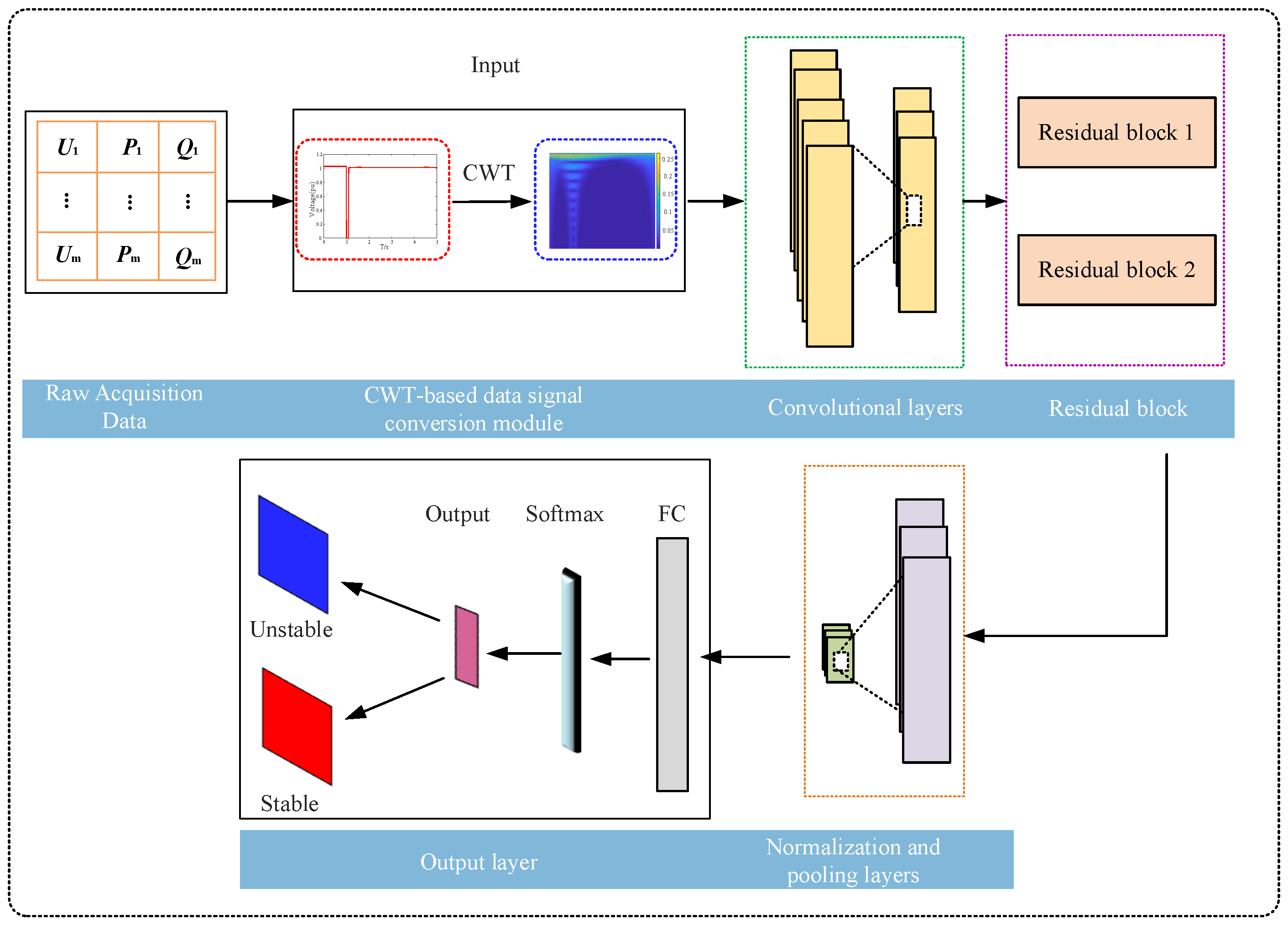
The overall network architecture for constructing the combined model is shown in Figure 1. It comprises an input module, a CWT feature extraction module, a ResNet feature learning module, a classification and stability assessment module, and a model validation and performance optimization module. First, the input layer acquires raw PMU measurement or simulation data. This data undergoes preprocessing before the CWT feature extraction module converts the voltage time-series signals into multi-scale time–frequency features via continuous wavelet transform. This generates a two-dimensional time–frequency matrix to capture local dynamics and frequency evolution characteristics during transient processes. Specific methodologies are detailed in Section 2. Subsequently, the ResNet feature learning module automatically extracts high-order abstract features from the time–frequency map through stacked convolutional layers and residual connections, mitigating the vanishing gradient problem in deep networks. Then, the classification and stability assessment module outputs stability classification results (e.g., stable/unstable) based on global average pooling (GAP) and fully connected layers, employing cross-entropy or focal loss functions to address sample category imbalance. Finally, a fully connected layer maps features captured by the preceding network to the output classification space. Probability values output via the ReLU activation function yield transient voltage stability/instability assessment results.

Figure 1. Hybrid model network architecture.

2.2. Continuous Wavelet Transform (CWT)

The continuous wavelet transform (CWT) is an effective time–frequency analysis method capable of capturing local features of transient voltage signals through multi-scale analysis. Its core principle involves decomposing voltage signals using scalable and shiftable wavelet basis functions to extract dynamic information about voltage disturbances across different scales and time windows. CWT transforms the input voltage signal into wavelet coefficients through a series of wavelet basis functions, forming a time–frequency distribution map. This process achieves scaling and translation of the original signal across different time and frequency scales.

Given the non-stationary and sudden nature of transient voltage disturbances (such as surges, dips, oscillations, harmonics, etc.), different wavelet basis functions exhibit varying capabilities in capturing signal characteristics. Therefore, selecting appropriate wavelet basis functions during transient voltage analysis enables more accurate extraction of the temporal location, duration, frequency components, and energy distribution of voltage disturbances.

The CWT method maps the energy distribution of voltage disturbances across different scales, thereby identifying characteristic information of transient voltage events. These wavelet coefficients reveal regions of concentrated energy within the voltage signal’s time–frequency domain, aiding in disturbance classification and assessment of their impact on power quality. Consequently, CWT provides an effective means for in-depth analysis of transient voltage characteristics. The CWT method is expressed as follows:

$$T(a,b)={\displaystyle \frac{1}{\sqrt{a}}}{\displaystyle {\int }_{-\infty }^{\infty }x(t){\psi }_{a,b}^{*}(t)dt}$$

(1)

where the shape and displacement of the wavelet function are determined by parameters a and b. a is the scaling factor reflecting frequency resolution; b is the translation factor reflecting time position; x(t) is the original signal; ${\psi }_{a,b}^{*}(t)$ is the complex conjugate of at parameters a and b; $T(a,b)$ is the continuous wavelet transform of the signal; when the wavelet is highly correlated with signal x(t) at given parameters a and b, a large magnitude $T(a,b)$ is obtained.

2.3. Deep Residual Modules

Deep learning networks are widely applied due to their effective handling of various feature extraction and classification tasks. Theoretically, increasing the depth of a deep learning network enhances its expressive power. However, in convolutional neural networks (CNNs), excessive depth leads to slower convergence and reduced accuracy. Even expanding the dataset to address overfitting does not improve classification performance or accuracy. Furthermore, as the network deepens and model parameters increase, issues like vanishing gradients or exploding gradients arise. The ResNet architecture was introduced to tackle the training challenges associated with traditional convolutional neural networks. This model employs identity mapping across multiple convolutional layers for backpropagation and parameter optimization, reducing training complexity. It effectively resolves the degradation issues in deep neural networks, accelerates convergence, and achieves strong performance in image recognition.

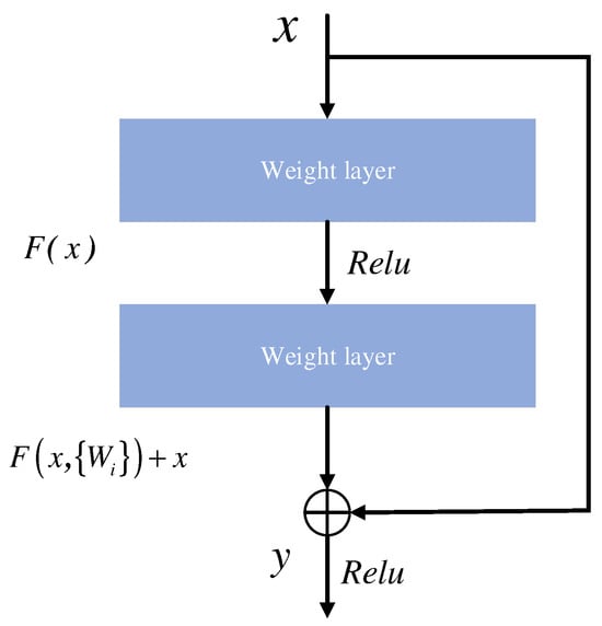
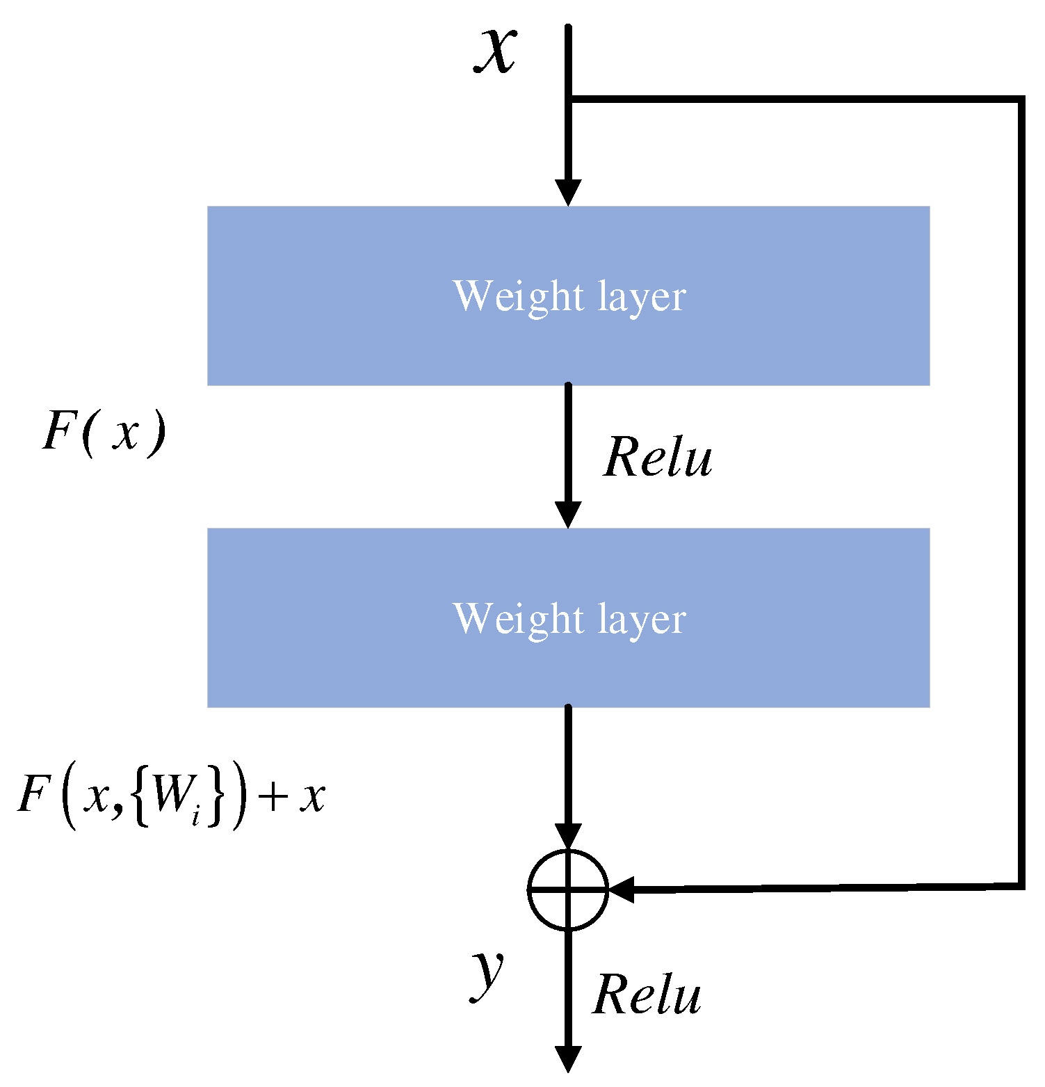
As one of the classic convolutional neural networks, the deep residual network incorporates multiple basic residual modules during its construction. These modules form the core component of the ResNet architecture. The residual block structure is illustrated in Figure 2, with its mathematical definition defined as

$$y=f\left(F\left(x,\left\{W_i\right\}\right)+x\right)$$

(2)

where x and y denote the input and output of the residual block; f represents the ReLU activation function; W_i denotes the weight parameters of the residual block; $F\left(x,\left\{W_i\right\}\right)$ indicates the residual mapping.

Figure 2. Residual module structure.

2.4. Deep Residual Network Architecture

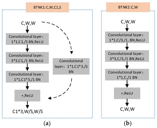
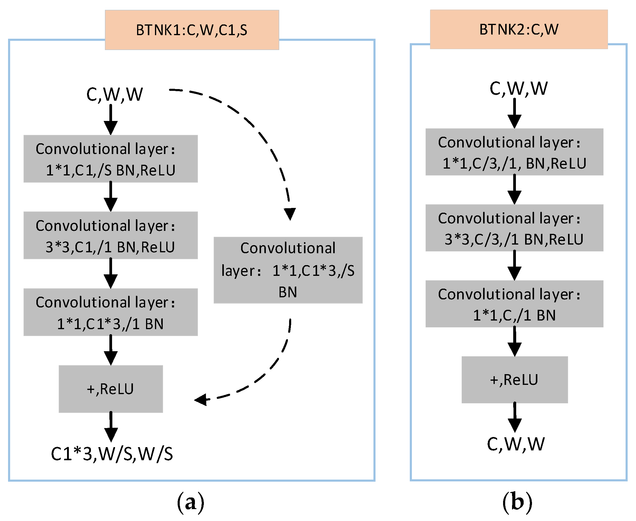
The overall architecture of ResNet is constructed based on a series of residual blocks. Different versions exist to meet varying application requirements, such as ResNet-18, ResNet-34, ResNet-50, ResNet-101, and ResNet-152. The primary distinctions between these variants lie in network depth and the types of residual blocks employed. The residual modules in ResNet-50 ensure network stability as layer count increases, effectively addressing the aforementioned challenges. ResNet-50s Bottleneck residual blocks comprise two types: Conv Block and Identity Block.

The residual module accepts inputs of dimensions C × W × W. It first performs a 1 × 1 convolution to reduce the feature image dimensions; this is followed by a 3 × 3 convolution operation, and finally, a 1 × 1 convolution restores the dimensions. The processed result is then fed into a batch normalization (BN) layer and a rectifying linear unit (ReLU) layer. At the dashed line, a C1 × 3 1 × 1 convolutional network reduces the output dimensions to C1 × 3, W/S, W/S. In Figure 3a, /S denotes stride, C and C1 represent channel counts, input image height and width are both W, BN indicates batch normalization, and ReLU is the activation function. The Identity Block, termed BTNK2 as shown in Figure 3b, bypasses dimensional reduction via convolutional networks. Instead, it directly adds the input to three convolutional blocks along with corresponding BN and ReLU operations, then passes through an activation function to produce the output.

Figure 3. Residual module structure. (a) Conv Block residual block. (b) Identity Block residual block.

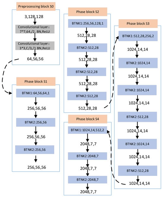
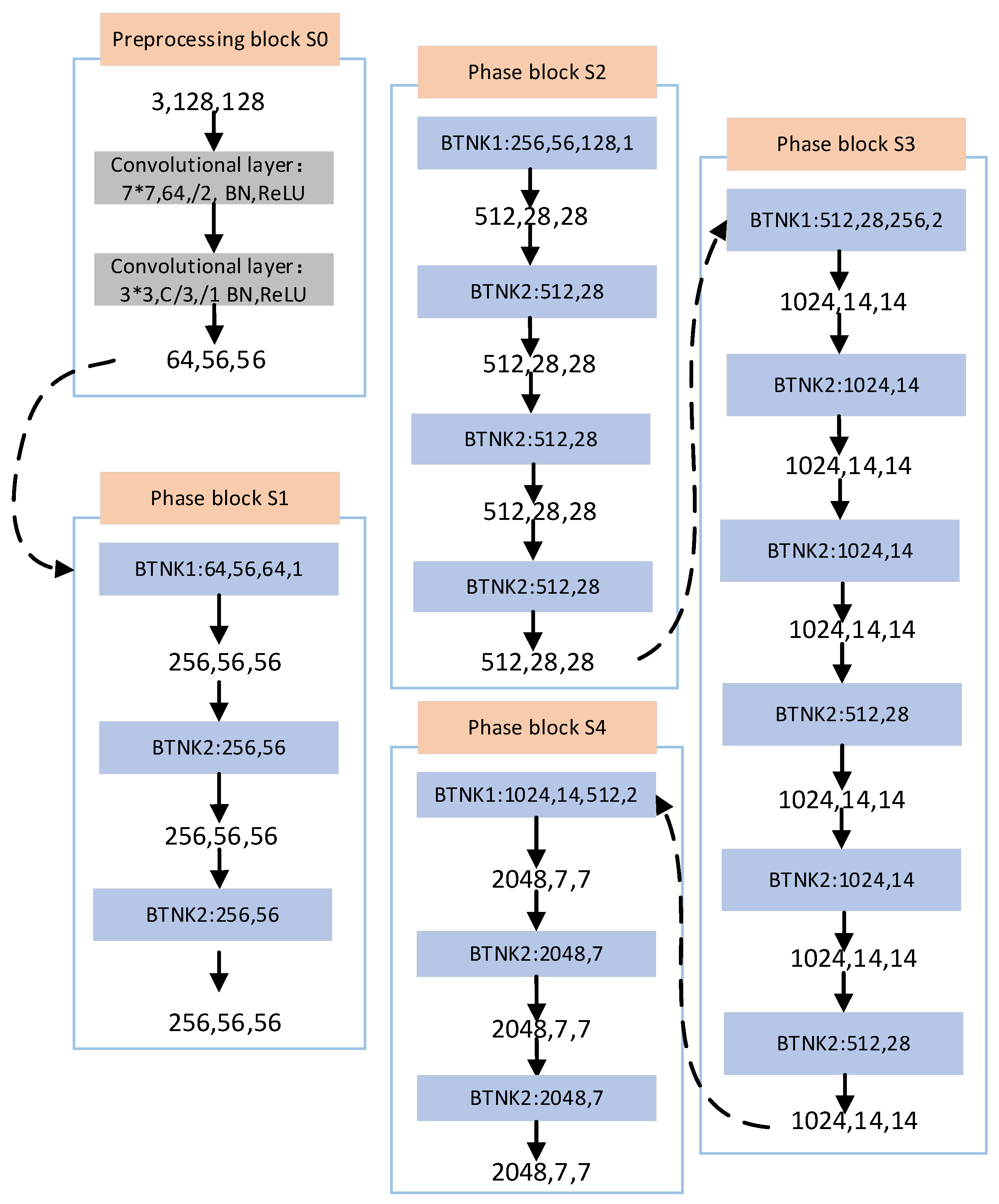
The ResNet-50 network architecture adopted in this study is illustrated in Figure 4. The network accepts a three-channel input of size 3 × 128 × 128, where the three channels correspond to the CWT time–frequency images of bus voltage, active power, and reactive power, respectively. In the S0 preprocessing block, the input first passes through a 7 × 7 convolutional layer with 64 filters and stride two (BN, ReLU), followed by 3 × 3 max-pooling with stride two, yielding a feature map of 64 × 56 × 56. This output then enters four stage blocks (S1–S4). S1 contains one Conv Block (BTNK1) and two Identity Blocks (BTNK2), expanding channels to 256 while maintaining spatial size at 56 × 56. S2 further expands channels to 512 with spatial resolution halved to 28 × 28. S3 and S4 continue this pattern, producing outputs of 1024 × 14 × 14 and 2048 × 7 × 7, respectively. The progressive channel expansion (64 → 256 → 512 → 1024 → 2048) and spatial down sampling across stages enable the network to extract increasingly abstract features from the CWT images. Throughout this process, shortcut connections allow gradients to flow directly through identity mappings, resolving the vanishing gradient problem inherent in very deep networks. ResNet-50 thus outperforms architectures such as VGG in both accuracy and computational efficiency, making it well-suited as the foundational backbone for transient voltage stability assessment in this study.

Figure 4. ResNet-50 network architecture.

3. Transient Voltage Stability Assessment Model

3.1. Sample Construction Process

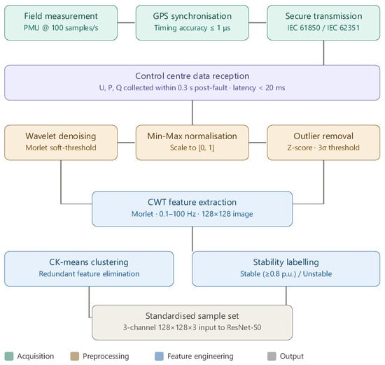
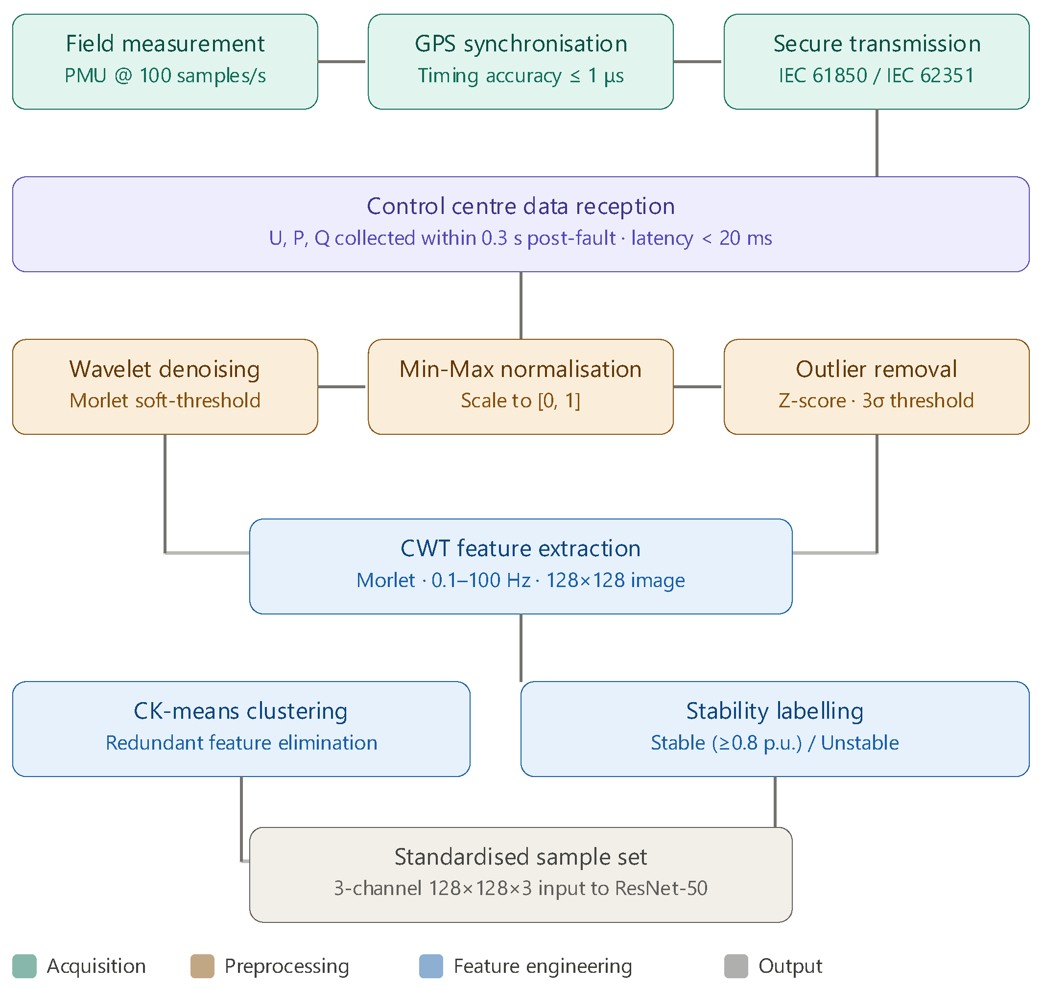
The sample construction process generates input features and labels through a systematic data processing workflow. Input features are derived from three key electrical quantities measured at the transmission points of renewable energy grids: bus voltages, active power, and reactive power. These signals are acquired via Phasor Measurement Units (PMUs), which synchronously sample at a rate of 100 samples/second using GPS-based time synchronization with timing accuracy within 1 microsecond, ensuring temporal consistency across geographically distributed measurement points [2]. The measured data is transmitted to the control center via IEC 61850-compliant communication protocols over fiber-optic networks, guaranteeing both real-time transmission (latency < 20 ms) and data integrity. To ensure data security, encryption mechanisms conforming to IEC 62351 standards are applied during transmission, preventing unauthorized access and data tampering.

Samples are collected within 0.3 s after fault clearance, capturing the critical transient recovery window. Raw data typically contains sensor noise and high-frequency interference; therefore, a Morlet wavelet soft-thresholding method is applied for denoising, followed by Min–Max normalization to scale all electrical quantities to the [0, 1] range. Outliers exceeding the 3σ threshold (Z-score method) are subsequently identified and removed. The complete data acquisition and preprocessing workflow is illustrated in Figure 5. The sample set can be represented as

$$X=\left[u_1,\cdots ,u_m,p_1,\cdots ,p_m,q_1,\cdots q_m\right]$$

(3)

where u_m represents bus voltages across the grid; p_m and q_m denote active and reactive power injected into lines and buses, respectively; and X is the output label for each sample.

Figure 5. Data acquisition and preprocessing framework for transient voltage stability assessment.

To cover diverse fault scenarios reflecting power system complexity, the simulation design incorporates typical fault types such as line short circuits, DC commutation failures, and load transients. Fault points are placed at the transmission end, receiving end, and intermediate nodes of renewable energy bases to simulate disturbance propagation characteristics across different regions. Setting fault clearance times (e.g., 50 ms, 100 ms, 200 ms) further reflects the dynamic fault recovery process, ensuring sample diversity.

During data preprocessing, raw data typically contains noise and dimensional differences, necessitating noise reduction and normalization to enhance data quality. A soft-thresholding method based on Morlet wavelets is employed to eliminate sensor noise and simulation errors. Electrical quantity data is then scaled to the [0, 1] range via Min–Max normalization, calculated as

$$x_{norm}={\displaystyle \frac{x-x_{\mathit{m}\mathit{i}\mathit{n}}}{x_{\mathit{m}\mathit{a}\mathit{x}}-x_{\mathit{m}\mathit{i}\mathit{n}}}}$$

(4)

where $x_{\mathit{m}\mathit{a}\mathit{x}}$ and $x_{\mathit{m}\mathit{i}\mathit{n}}$ denote the minimum and maximum values of the data, respectively. Additionally, the Z-score method identifies and removes outliers exceeding the 3σ range to ensure a reasonable data distribution.

Feature extraction and CWT-based time–frequency image generation form the core of sample construction. Traditional time-series data cannot be directly input into deep learning models; thus, CWT conversion to time–frequency images is essential for extracting dynamic features. The Morlet wavelet basis function is selected due to its strong localization capability for oscillatory signals, making it suitable for capturing non-stationary features such as voltage surges/drops and harmonics. The scale range is set from 0.1 to 100 Hz, covering the power system’s fundamental frequency (50 Hz) and its harmonics, ensuring both low-frequency and high-frequency features are extracted. The CWT coefficient matrix is converted into a 128 × 128 grayscale image via grayscale mapping, with pixel values ranging from [0, 255] corresponding to linear interpolation of coefficient amplitudes. For multi-channel inputs, CWT images of voltage, active power, reactive power, and load current are concatenated to form a three-channel image (128 × 128 × 3), preserving the coupling relationships among multidimensional electrical quantities.

3.2. Transient Voltage Stability Criteria

In the classification of sample output labels, according to the Guidelines for Power System Security and Stability, if the node voltage recovers to 0.8 p.u. or above within 10 s after a fault, and the voltage at the 220 kV and above central nodes remains no lower than 0.9 p.u., it is recorded as “stable” (Label 2); if the node voltage fails to recover to 0.8 p.u. within 10 s, or the central node voltage remains below 0.9 p.u. for over 1 s, it is classified as “unstable” (Label 1). The label generation process includes sliding window analysis (window length = 10 s), criterion matching, and cross-validation to ensure label definitions align with time-domain simulation results.

3.3. Handling Data Imbalance

Since actual power systems operate stably most of the time, the number of collected unstable samples is typically fewer than stable samples, resulting in data imbalance [20]. In this article, ‘stable’ refers to the ability of the voltage at each node to recover to an acceptable level within a specified time after a fault—in particular, if the node voltage recovers to 0.8 p.u. or above within 10 s after a fault, and the voltage of central nodes at 220 kV and above is not lower than 0.9 p.u., it is considered ‘stable’; otherwise, it is ‘unstable’. In a sample space with imbalanced class distribution, evaluation models struggle to fully learn the feature information of minority class samples, affecting the overall evaluation performance of the model. The standard focal loss (FL), originally proposed by Lin et al., modulates the gradient update direction through a focusing factor to enhance focus on hard-to-classify samples, thereby improving the model’s handling of imbalanced data. However, standard FL was designed primarily to suppress easy-sample dominance at the sample level, without accounting for dataset-level class frequency distribution. Its calculation formula is

$$\mathrm{FL}(p,y)=-{(1-p)}^{\gamma }\mathit{l}\mathit{o}\mathit{g}(p_i)$$

(5)

where γ is the modulation factor for easy/hard samples; $p_i$ is the model’s predicted probability for the target class.

Although FL effectively addresses hard-to-classify samples, it fails to dynamically optimize loss weights under extreme imbalance; consequently, the dominance of the majority class may obscure the discrimination of the minority class. This paper introduces a category–number balancing factor ${\lambda }_i$ to dynamically optimize loss weights across categories, yielding the improved FL formula

$${\mathrm{FL}}^{\prime }(p,y)=-{\displaystyle \sum _{i=1}^n{(1-p)}^{{\lambda }_i\gamma }\mathit{l}\mathit{o}\mathit{g}(p_i)}$$

(6)

where the category–number balancing factor λ_i is expressed as

$${\lambda }_i=\sqrt{{\displaystyle \frac{C_i}{{\displaystyle \sum _{j=1}^k{C}_j}}}}$$

(7)

where $C_i$ denotes the number of samples in category $i$; k is the total number of categories. Unlike the standard FL which relies solely on the per-sample focusing factor ${(1-p)}^{\gamma }$, the improved FL additionally incorporates ${\lambda }_i$ to compensate for dataset-level class frequency skew. The square-root formulation in Equation (7) is deliberately chosen to avoid over-correction: a linear inverse-frequency weight would excessively amplify minority-class gradients, whereas the square root provides moderate compensation that preserves the balance between classification difficulty and distributional skew. Consequently, the improved FL simultaneously addresses both sample-level hard-example mining and dataset-level class imbalance, which standard FL alone cannot achieve.

3.4. Model Evaluation Metrics

To comprehensively evaluate the transient voltage assessment model’s performance, this paper employs a confusion matrix and defines four key performance metrics: accuracy (Ac), precision (Pr), recall (Re), and confusion matrix. The confusion matrix is shown in Table 1. Beyond conventional accuracy measures, the $F_1$ score reflects the model’s predictive capability for unstable samples.

Table 1. TSA confusion matrix.

Predicted Value	Actual
	Stable	Unstable
Stable	$T_P$	$F_P$
Unstable	$F_N$	$T_N$

The expression is as follows:

$$A_C={\displaystyle \frac{T_P+T_N}{T_P+T_N+F_P+F_N}}$$

(8)

$$P_r={\displaystyle \frac{T_N}{T_N+F_N}}$$

(9)

$$R_e={\displaystyle \frac{T_N}{T_N+F_P}}$$

(10)

$$F_1={\displaystyle \frac{2\times P_r\times R_e}{P_r+R_e}}$$

(11)

where $F_P$ and $T_P$ represent the number of samples incorrectly and correctly assessed as unstable, respectively; $F_N$ and $T_N$ represent the number of samples incorrectly and correctly assessed as stable, respectively.

3.5. CWT-ResNet-Based Transient Voltage Stability Assessment Workflow

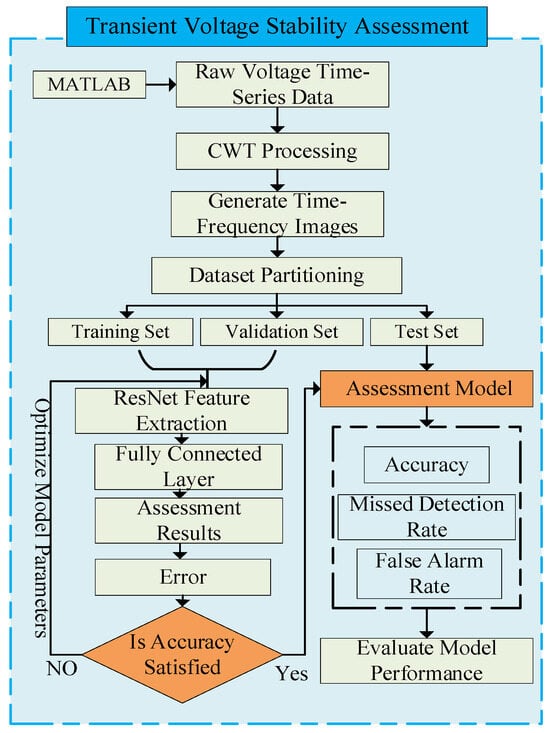
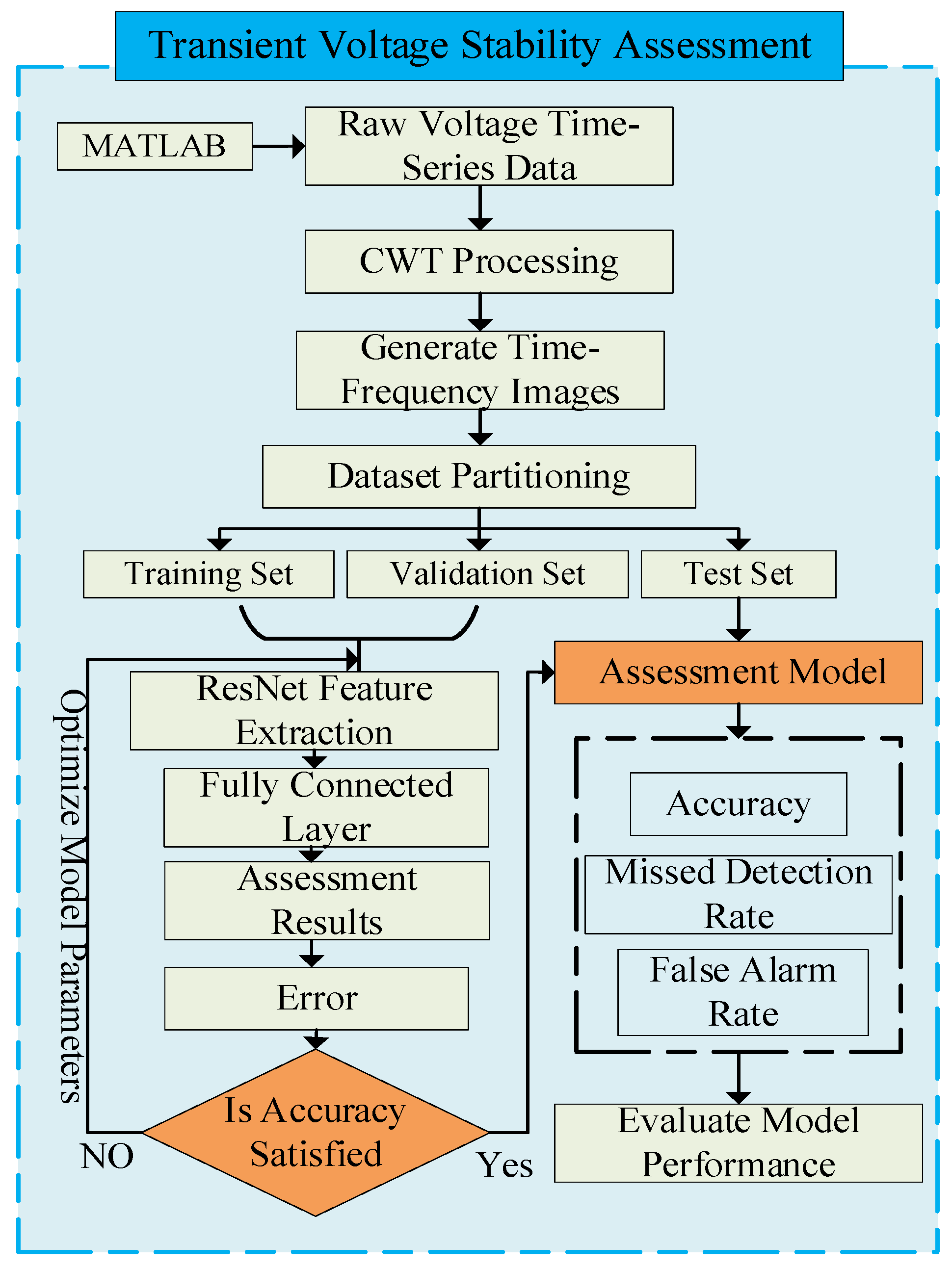
The specific workflow of the CWT-ResNet-based transient voltage stability assessment method is illustrated in Figure 6.

Figure 6. CWT-ResNet transient voltage stability assessment workflow.

Step 1: Data Acquisition and Standardized Preprocessing. In practical deployment, raw time-series data is obtained via PMU (Phasor Measurement Unit) devices installed at key transmission buses, which record three-phase voltage phasors, active power, and reactive power at a sampling rate of no less than 100 Hz in compliance with IEEE Std C37.118.1. Upon detection of a disturbance event, a 0.3 s post-fault data window is captured and transmitted to the control center via the Phasor Data Concentrator (PDC) over fiber-optic communication links. In offline training scenarios, equivalent data can be obtained from fault simulations. Sensor noise and high-frequency interference are then eliminated using the Morlet wavelet soft-thresholding method. Min–Max normalization is subsequently applied. Finally, outliers are identified and removed based on the Z-score criterion, yielding a standardized time-series sample set that establishes the data foundation for feature extraction.

Step 2: Time–Frequency Feature Extraction. Continuous wavelet transform (CWT) is independently applied to key time-series signals within each preprocessed sample—bus voltage and line active/reactive power. This step is computationally lightweight and can be executed in real time on a standard industrial server or edge computing node at the control center, typically within 20–50 ms.

Step 3: Time–Frequency Image Generation. Univariate time series are transformed into time–frequency matrices via CWT using the Morlet wavelet basis over 0.1–100 Hz scales. The Morlet wavelet is chosen for its optimal time–frequency localization and ability to capture the oscillatory nature of transient voltage signals; the 0.1–100 Hz range covers all dynamically significant phenomena in the study system, from inter-area oscillation modes (0.1–0.7 Hz) and control dynamics (1–10 Hz) to the fundamental frequency (50 Hz) and UHVDC commutation-related second harmonics (100 Hz). CWT coefficient matrices are mapped to 128 × 128 grayscale images through linear interpolation, forming single-channel time–frequency images; this resolution was determined through comparative experiments across candidate sizes (64 × 64, 128 × 128, and 256 × 256), where 128 × 128 achieved the best balance between classification accuracy and computational efficiency. Voltage, active power, and reactive power images are concatenated to form a three-channel (128 × 128 × 3) input tensor, preserving multidimensional coupling features.

Step 4: Deep Feature Extraction. ResNet-50 is selected as the multi-channel image input network. Features are extracted through convolutional layers and residual blocks, then compressed into feature vectors via global average pooling. An improved focal loss function is introduced to dynamically adjust loss weights across different categories. The pre-trained model requires only a CPU-equipped server for real-time inference, with no specialized hardware beyond standard control center computing infrastructure.

Step 5: Stability Classification and Output. The model outputs stability classification results (stable/unstable) via global average pooling and a fully connected layer, with inference completing in under 10 ms. The total end-to-end latency from disturbance onset to classification output is estimated at under 200 ms, satisfying the operational requirements for online emergency voltage control. Predicted probability values are mapped to the [0, 1] range using the ReLU activation function.

Step 6: Results and Performance Validation. Accuracy (Ac), precision (Pr), and recall (Re) are calculated using a confusion matrix. Model performance is validated across diverse category datasets to ensure robustness in extremely imbalanced data scenarios. In online operation, the classification result and predicted probability are transmitted to the Energy Management System (EMS) dispatcher interface to support real-time decision-making.

4. Case Study Analysis

4.1. Sample Set Construction

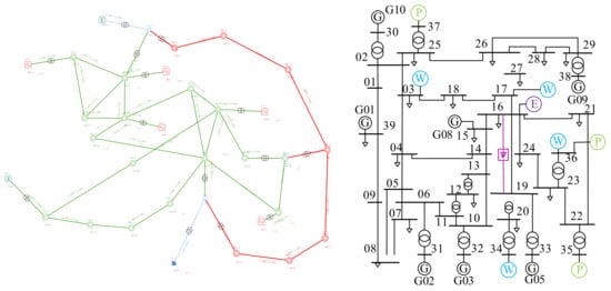
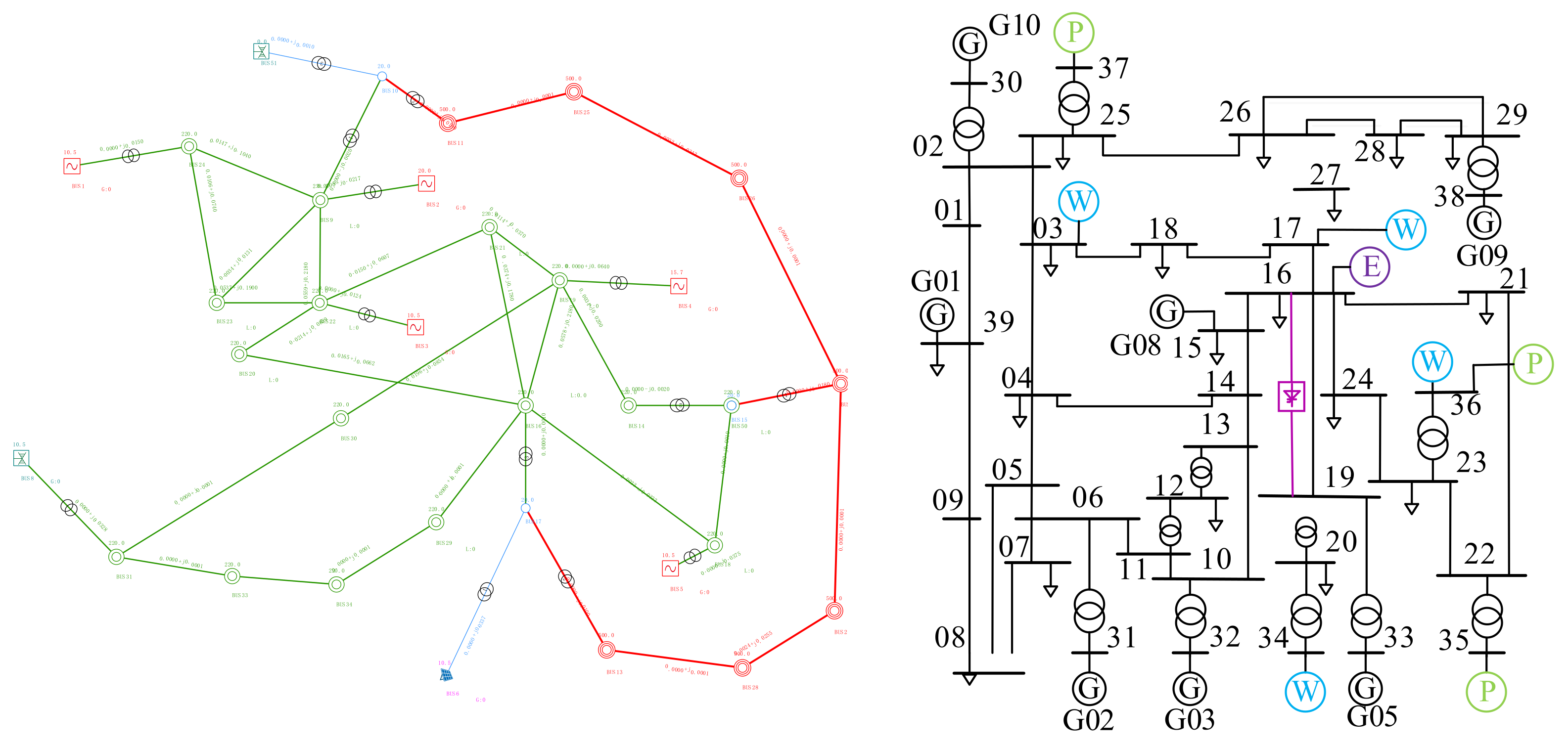
Taking the Qishao DC transmission line in Northwest China as an example, a simulation model of the IEEE 10-machine 39-node system was constructed based on PSASP, with the structure shown in Figure 7. The IEEE 10-machine 39-node system was modified by adding a DC transmission line between nodes 16 and 19, installing wind farms at nodes 03, 17, 34, and 36, photovoltaic power plants at nodes 37, 35, and 36, and a responsive energy storage system at node 16. This configuration enables transient voltage stability assessment. Within the system model, generators employ a second-order classical model, while loads adopt a constant impedance mode. To generate training data, diverse simulation data were produced by altering system operating states and fault conditions. For comparative analysis, power flow non-convergence cases were filtered out during data preprocessing, yielding 1490 valid samples—998 transient stable samples and 492 transient unstable samples—maintaining a sample ratio of approximately 3:1.

Figure 7. IEEE 10-machine 39-node system and Gansu power grid topology.

The deep learning model was constructed in the MATLAB 2023b environment. The hardware configuration comprised an Intel^® Core™ i7-8700 CPU @ 3.20 GHz (base frequency 3.19 GHz) with 8 GB RAM.

4.2. Data Generation and Preprocessing

To fully account for diverse fault scenarios in actual power grids and enhance training sample diversity, Datasets A and B were generated by setting different simulation conditions. Dataset A was created under N-1 fault conditions by varying load levels to 95%, 100%, and 105%. The fault location was varied at 10%, 20%, 30%, 40%, 50%, 60%, 70%, 80%, 90%, and 100%. The fault duration was varied at 0.1 s, 0.15 s, 0.2 s, 0.25 s, and 0.3 s. Dataset B is obtained under identical conditions with a DC lockout fault applied. Specific time-domain simulation parameters are detailed in Table 2.

Table 2. Time-domain simulation parameter settings.

Parameter Category	Parameter Value	Number of Parameters
Frequency	50 Hz	1
DC	16–19	1
Fault Type	DC Lockout, N-1 Fault	2
Load Level	95%, 100%, 105%	3
Fault Location	10%, 20%, 30%, 40%, 50%, 60%, 70%, 80%, 90%, 100%	10
Fault Duration	0.1, 0.15, 0.2, 0.25, 0.3	5

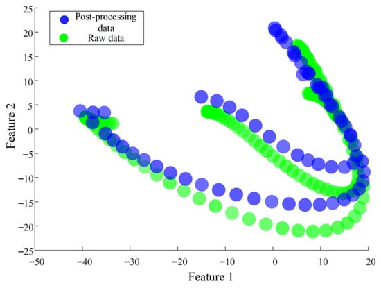
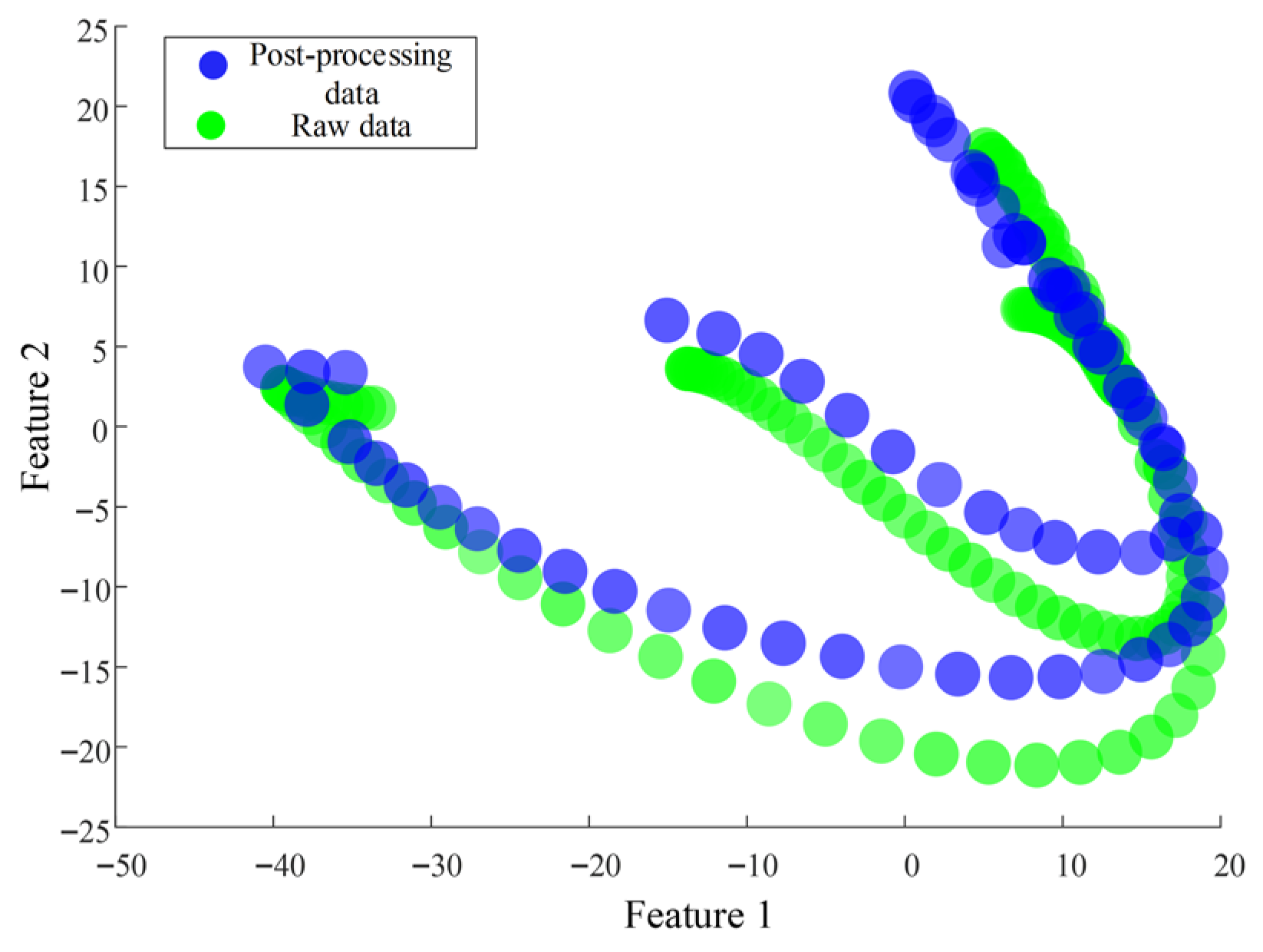
Bus voltages, line active power, and line reactive power were collected from the aforementioned time-domain simulations. To enhance the accuracy of the model training dataset, CK-means clustering was applied to line active power and reactive power data to eliminate redundant features providing minimal information for voltage stability. PCA visualization was performed on both the original and clustered datasets, as shown in Figure 8.

Figure 8. PCA visualization of dataset before and after CK-means redundant feature elimination.

As shown in the Figure 8, this method clusters stable and unstable datasets. Merging all clustered data reveals that the original data points are green, while the clustered data points are blue. The number of blue points is significantly reduced compared to green points, indicating that redundant data has been effectively reduced through this method. After data reduction, the continuous wavelet transform (CWT) algorithm was applied to convert the acquired time-series data signals into two-dimensional time–frequency images.

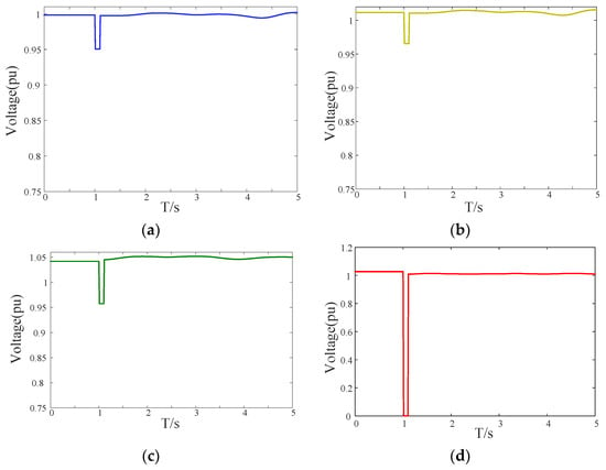
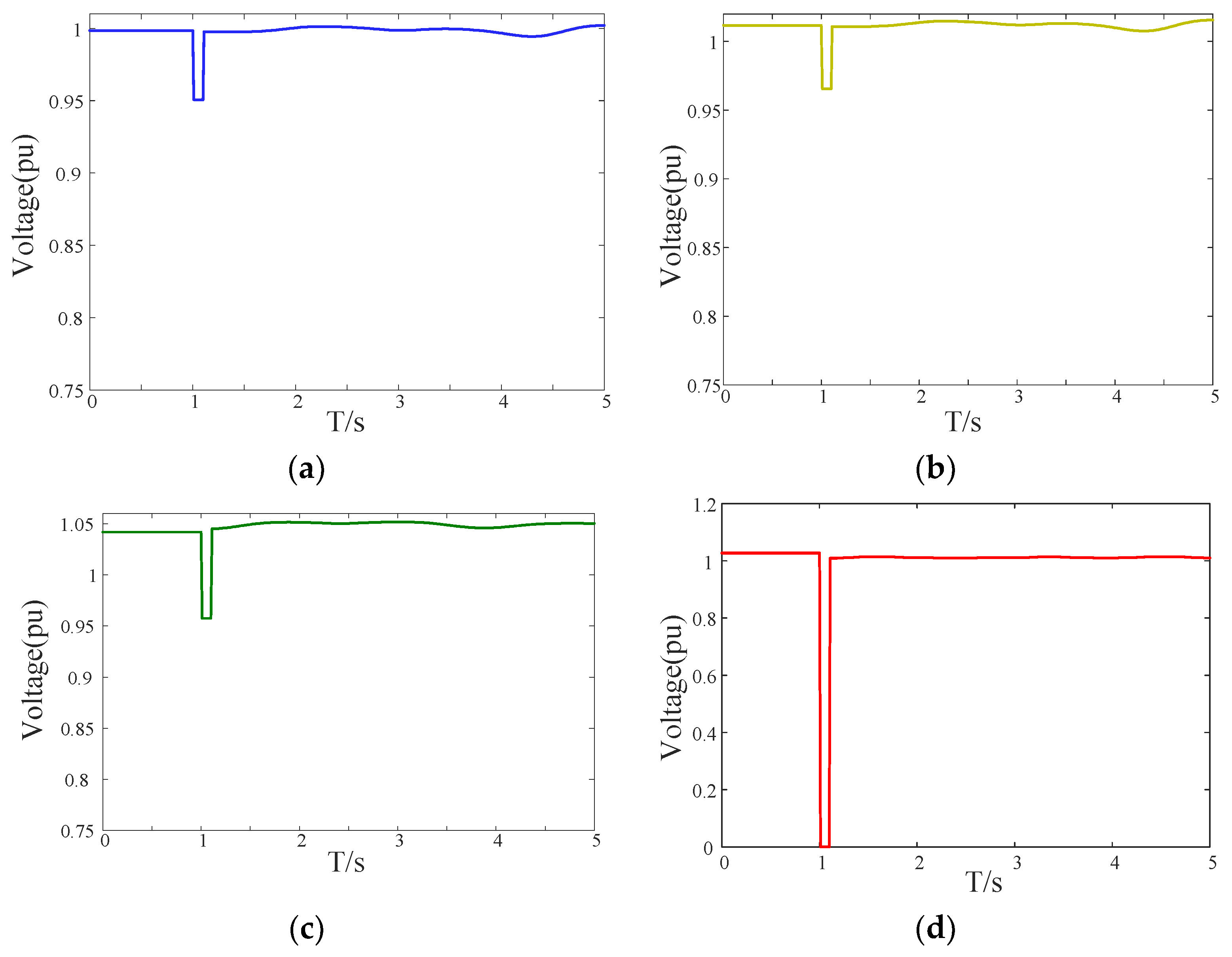
The data underwent signal-to-image conversion via CWT. The post-fault bus voltages of nodes BUS1, BUS11, BUS12, and BUS37 in Dataset A were selected, as shown in Figure 9. All voltage waveforms exhibit a sudden drop at the fault instant t = 0.2 s. However, significant differences were observed in the recovery speed and final steady-state values post-fault. The voltage of BUS11 recovered to above 0.8 p.u. within 0.3 s, whereas the recovery time for BUS37 exceeded 0.5 s with a final value below the threshold. These differences in characteristics provide crucial information for two-dimensional image features.

Figure 9. Bus voltages at various nodes. (a) BUS1 bus voltage. (b) BUS11 bus voltage. (c) BUS12 bus voltage. (d) BUS37 bus voltage.

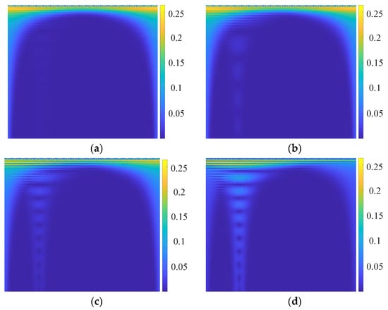
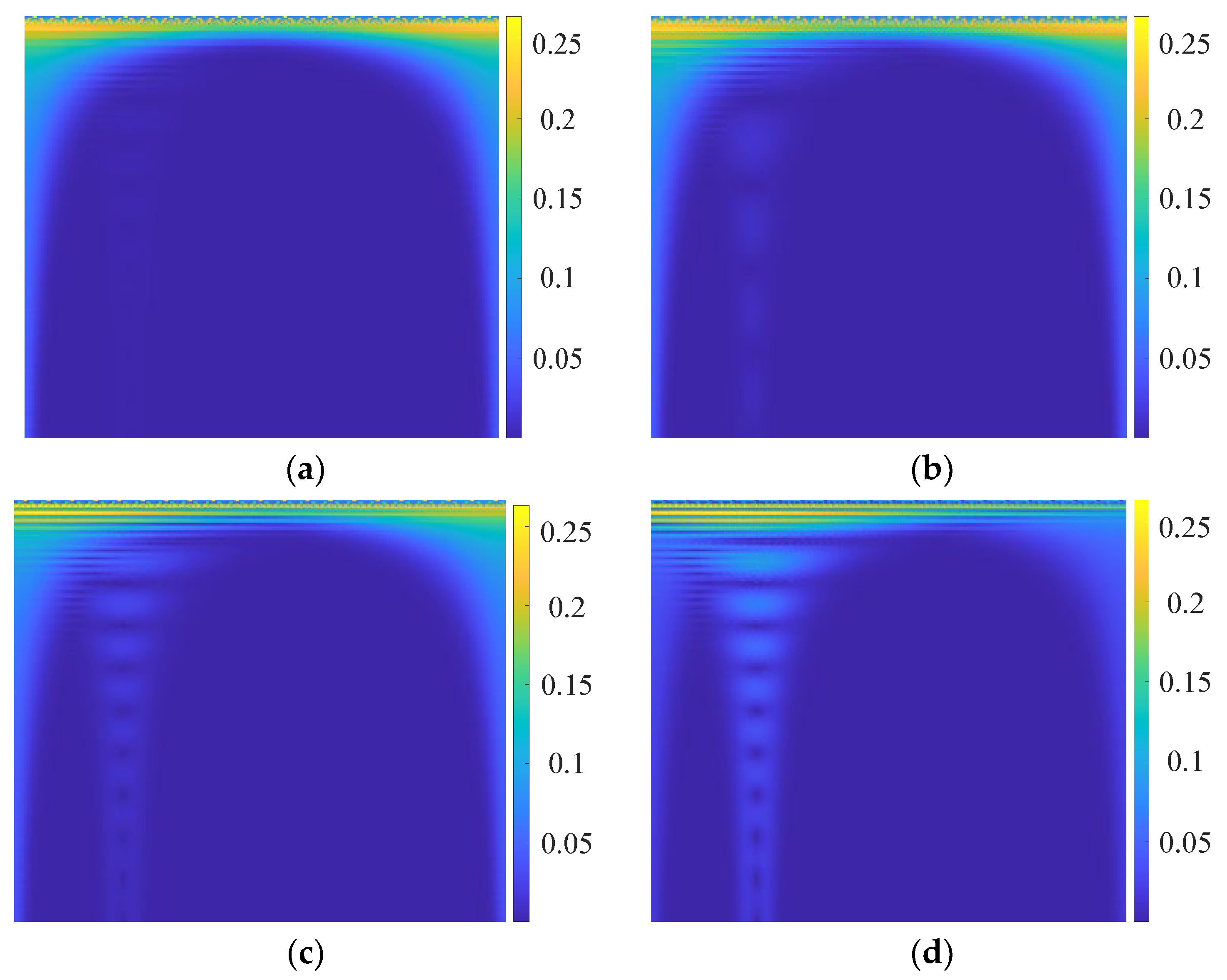
Figure 10a–d present the two-dimensional time–frequency representations of voltage signals, obtained using the Morlet wavelet basis to capture characteristics such as voltage swells/sags and harmonic components. The time–frequency images of BUS11 exhibit energy concentrated at high-frequency scales, presenting distinct “spike” characteristics with rapid attenuation in disturbed regions, indicating its fast recovery capability. In contrast, the BUS37 image exhibits prolonged low-frequency disturbance duration with dispersed energy distribution, forming a “tailing” effect. Noticeable color changes occur in the disturbed region, indicating unstable characteristics. These image features reveal the dynamic properties of voltage disturbances while providing rich textural information for ResNet-50’s convolutional operations, thereby enhancing classification performance.

Figure 10. CWT-processed voltage image features for BUS1, 11, 12, and 37. (a) BUS1 bus voltage image features. (b) BUS11 bus voltage image features. (c) BUS12 bus voltage image feature. (d) BUS37 bus voltage image feature.

4.3. Model Training Results

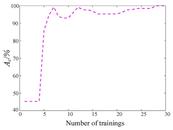
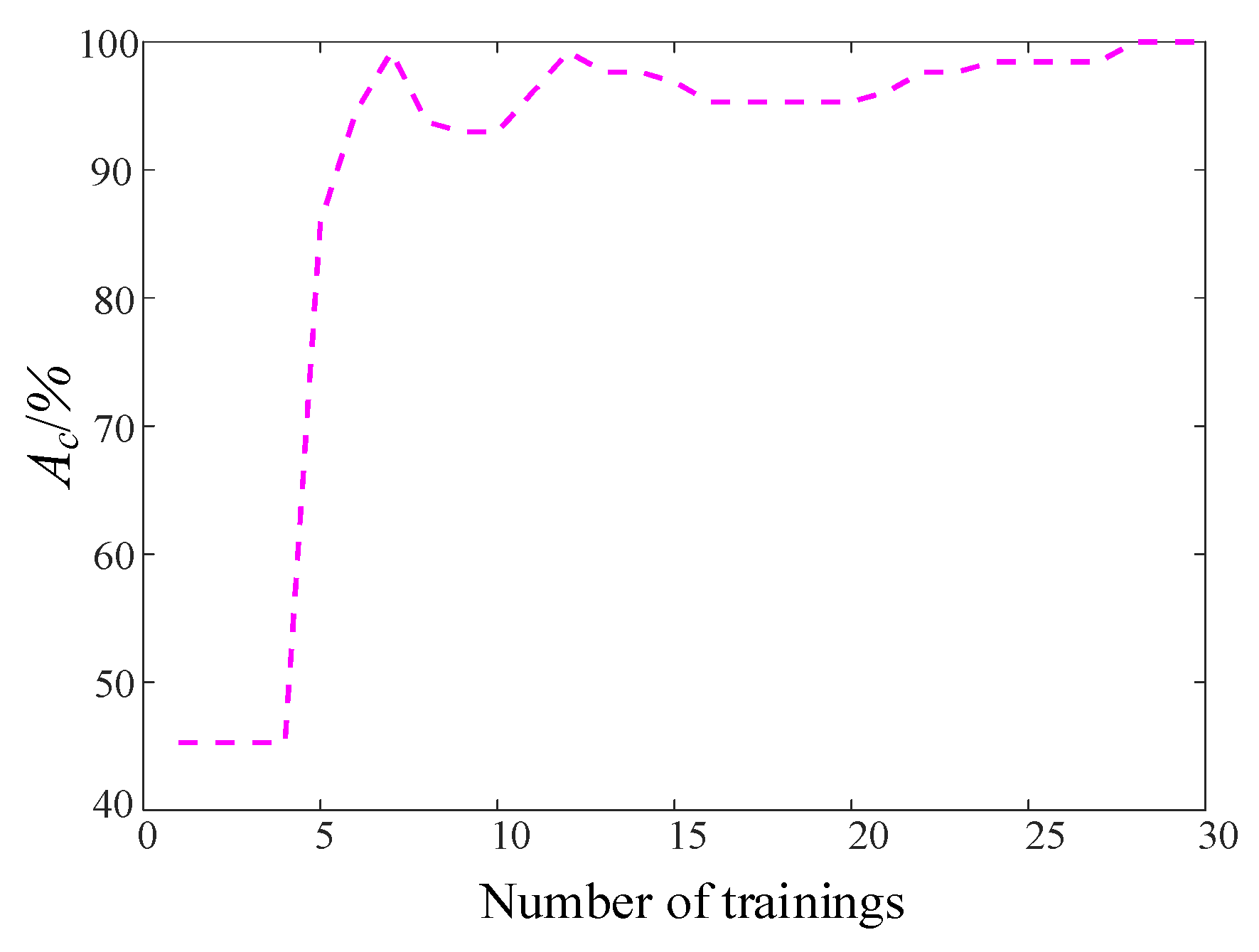
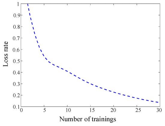
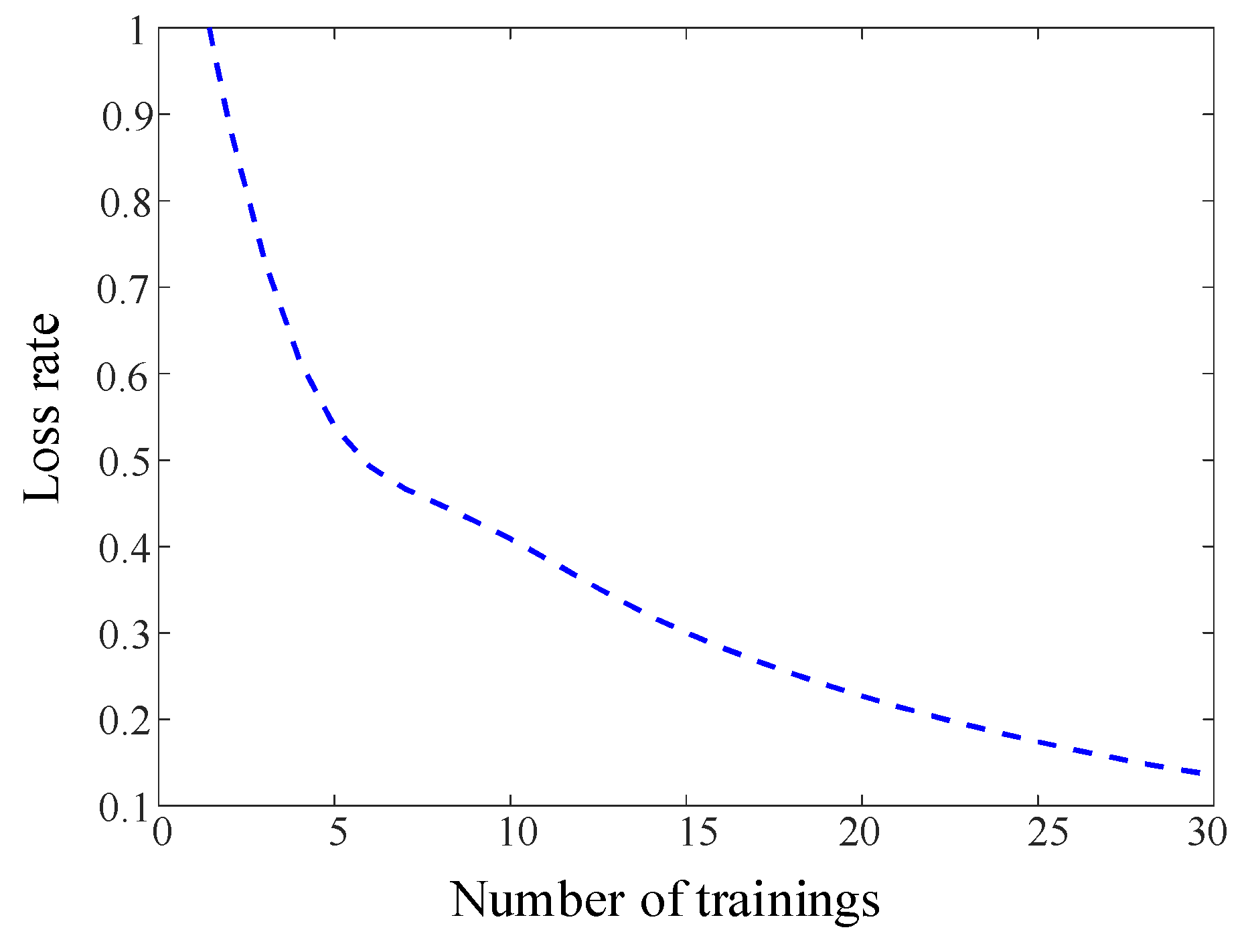
The hyperparameters affecting model evaluation include initial learning rate, convolution size, and training iterations. During ResNet model training, the Adam optimization algorithm was employed with a maximum of 30 training iterations, a gradient threshold of one, an initial learning rate of 0.001, and a learning rate adjustment factor of 0.01. As training progressed, the model’s accuracy showed an upward trend while the loss value decreased, as illustrated in Figure 11 and Figure 12. The accuracy curve converged rapidly and stabilized after approximately 11 epochs, ultimately reaching 98.88% accuracy. This indicates the model possesses excellent fitting capability without overfitting. The loss value rapidly decreased from an initial 0.5 to below 0.15 and remained stable, indicating that the improved focused loss (FL) function effectively mitigated the class imbalance issue. Furthermore, the residual structure of ResNet was verified to reduce the training difficulty of deep networks, enabling the model to rapidly extract key features. This demonstrates the high efficiency and robustness of CWT-ResNet in transient voltage stability assessment.

Figure 11. Training accuracy curve of the proposed CWT-ResNet model during the learning process.

Figure 12. Training loss curve of the proposed CWT-ResNet model during the learning process.

4.4. Model Performance and Feature Visualization Analysis

To validate the effectiveness of the proposed evaluation method, it was compared with mainstream deep learning models such as support vector machines (SVMs), one-dimensional convolutional neural networks (CNNs), and one-dimensional Residual Neural Networks. The specific evaluation performance results for each model are shown in Table 3.

Table 3. Model performance evaluation comparison.

Model	Ac/%	Pr/%	Re/%	F1/%
SVM	91.57 ± 1.32	100± 0.00	52.94 ± 0.17	68.42 ± 2.65
CNN	95.77 ± 0.94	94.22 ± 1.28	98.15 ± 0.85	96.15 ± 0.97
1D-ResNet	98.42 ± 0.46	100 ± 0.00	93.65 ± 1.08	96.72 ± 0.64
CWT-ResNet	98.88 ± 0.27	94.74 ± 0.72	100 ± 0.00	97.29 ± 0.41

As shown in Table 3, the proposed CWT-ResNet consistently outperforms all compared methods across all metrics, while exhibiting the smallest standard deviation (Ac: ±0.27%), indicating superior stability across different data partitions. Compared with the one-dimensional ResNet, which shares a similar backbone architecture, CWT-ResNet achieves a further improvement of 0.46% in Ac and 0.57% in F1, demonstrating that the two-dimensional time–frequency representation introduced by CWT provides richer discriminative features beyond what one-dimensional residual structures can capture. Traditional shallow methods such as SVMs show markedly lower recall (52.94%), reflecting their inability to model the nonlinear dynamics inherent in transient voltage trajectories. While the CNN improves upon SVMs by learning local temporal patterns, it remains constrained to a single time-domain view and achieves lower Ac (95.77%) compared with residual architectures. In contrast, CWT-ResNet converts voltage time series into multi-scale time–frequency images, enabling simultaneous extraction of temporal and spectral transient features that neither pure time-domain CNN models nor 1D-ResNet architectures can fully capture. The improved FL function further contributes to stable performance under class imbalance, as evidenced by the perfect recall (100%) and the lowest F1 standard deviation (±0.41%) among all compared methods.

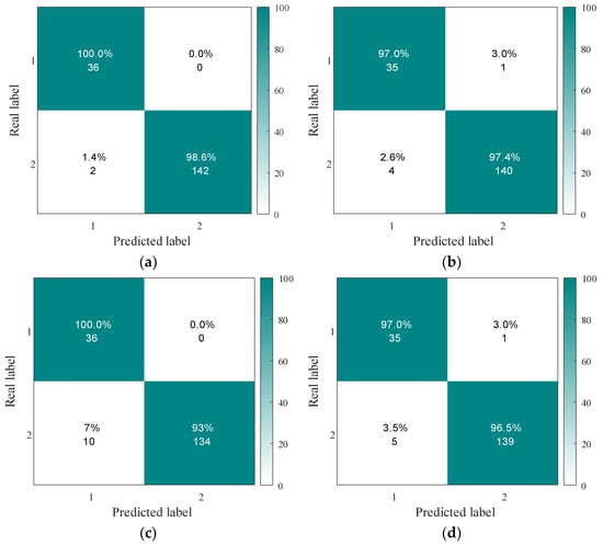
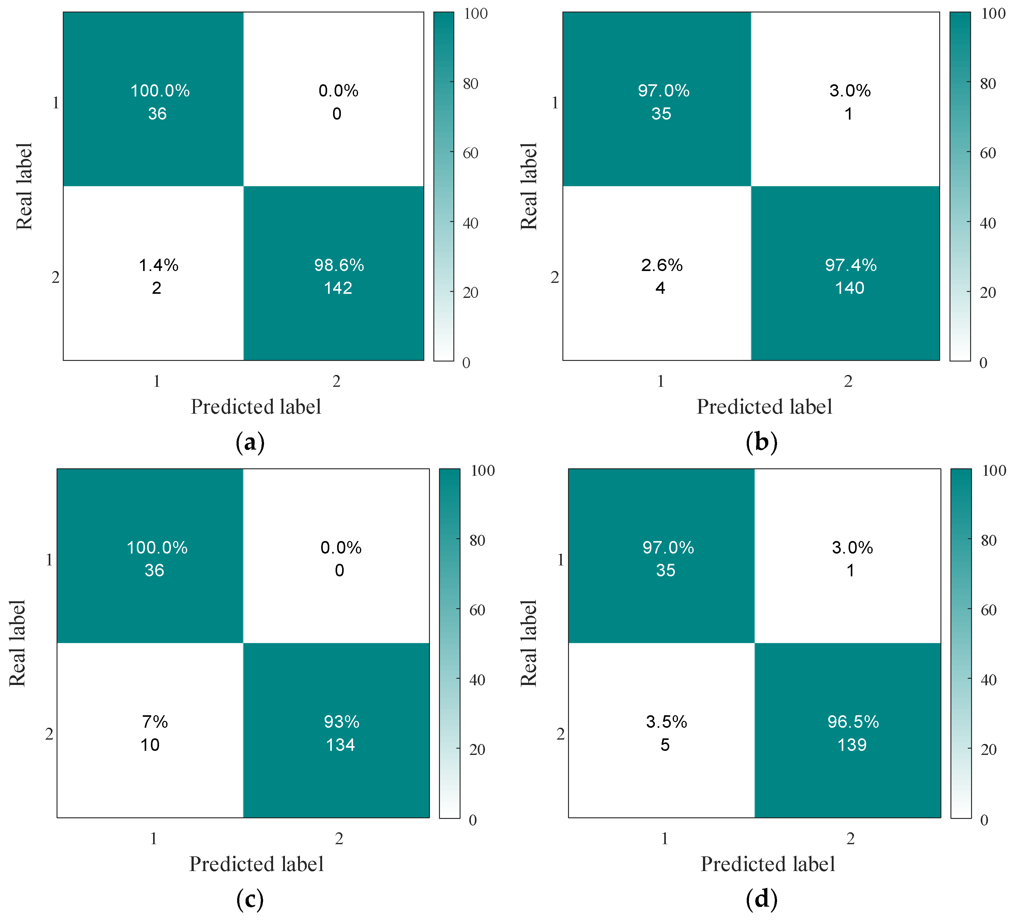
To analyze the effectiveness of the FL function in voltage stability assessment, the confusion matrices of four schemes—cross-entropy, weighted cross-entropy, focal loss (FL), and improved FL—were compared, as shown in Figure 13. Stability is represented as two, while instability is represented as one. The accuracy of the improved FL, A_c = 98.88%, improved by 1.66% and significantly outperformed other methods, demonstrating particularly outstanding performance in identifying unstable samples, as detailed in Table 4. In contrast, the traditional cross-entropy method achieved only 87.80% for R_e and 92.10% for P_r, indicating higher misclassification rates for minority samples. While weighted cross-entropy improved R_e to 92.10% by increasing the weight of unstable samples, P_r decreased to 89.70%, resulting in overall suboptimal performance. The improved FL introduces a dynamic focus factor that reduces the loss contribution from easily classified samples while increasing attention to hard-to-classify samples. This balances stable and unstable samples, thereby enhancing the model’s evaluation performance.

Figure 13. Confusion matrices for different schemes. (a) Improved focal loss function. (b) Focal loss function. (c) Cross-loss function. (d) Weighted cross-loss function.

Table 4. Evaluation results for different schemes.

Loss Function	Ac/%	Pr/%	Re/%	F1/%
Cross-entropy	94.44	78.26	100	87.80
Weighted cross-entropy	96.67	87.5	97.22	92.10
FL	97.22	89.74	97.22	93.33
Improved FL	98.88	94.74	100	97.29

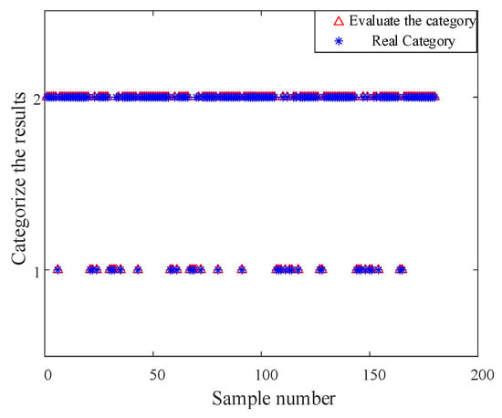
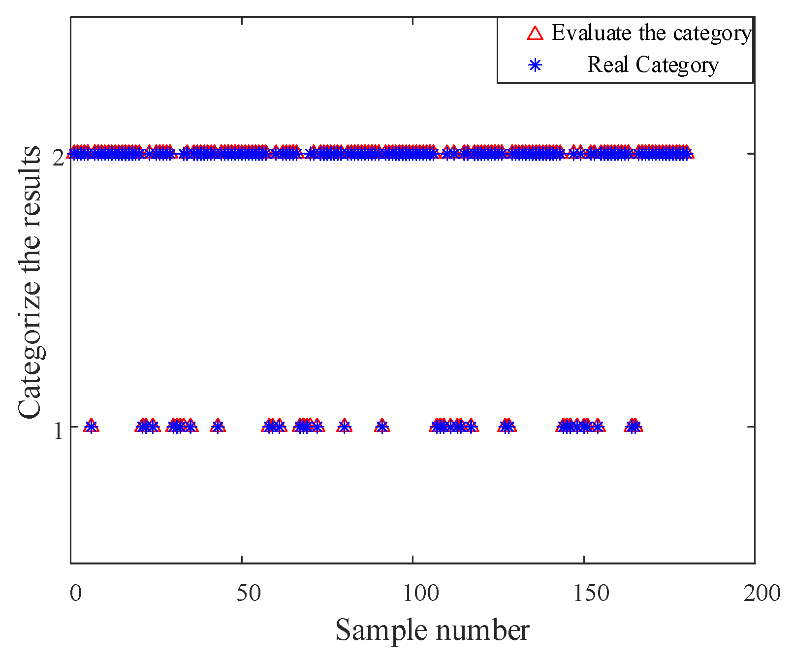
To more intuitively demonstrate the model’s evaluation capability on samples, we analyze the assessment results for stable and unstable samples, as shown in Figure 14. The figure indicates that in the stable category, triangles and stars do not correspond one-to-one, suggesting misclassifications in stable category evaluations. This validates the results from the confusion matrix mentioned above.

Figure 14. CWT-ResNet network evaluation results.

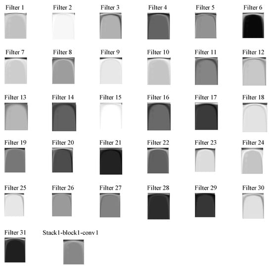
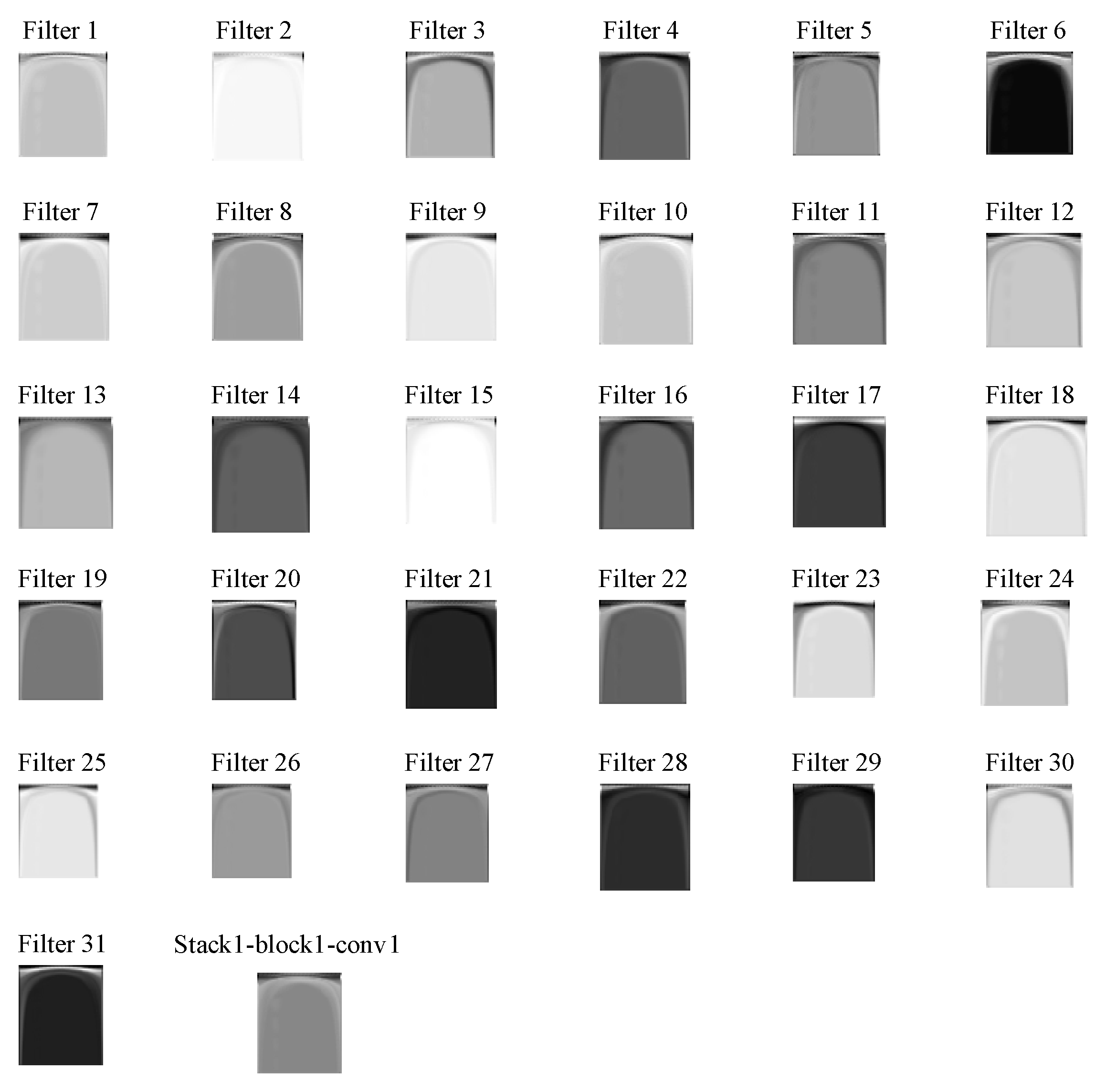
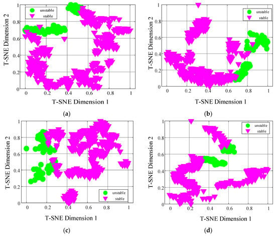
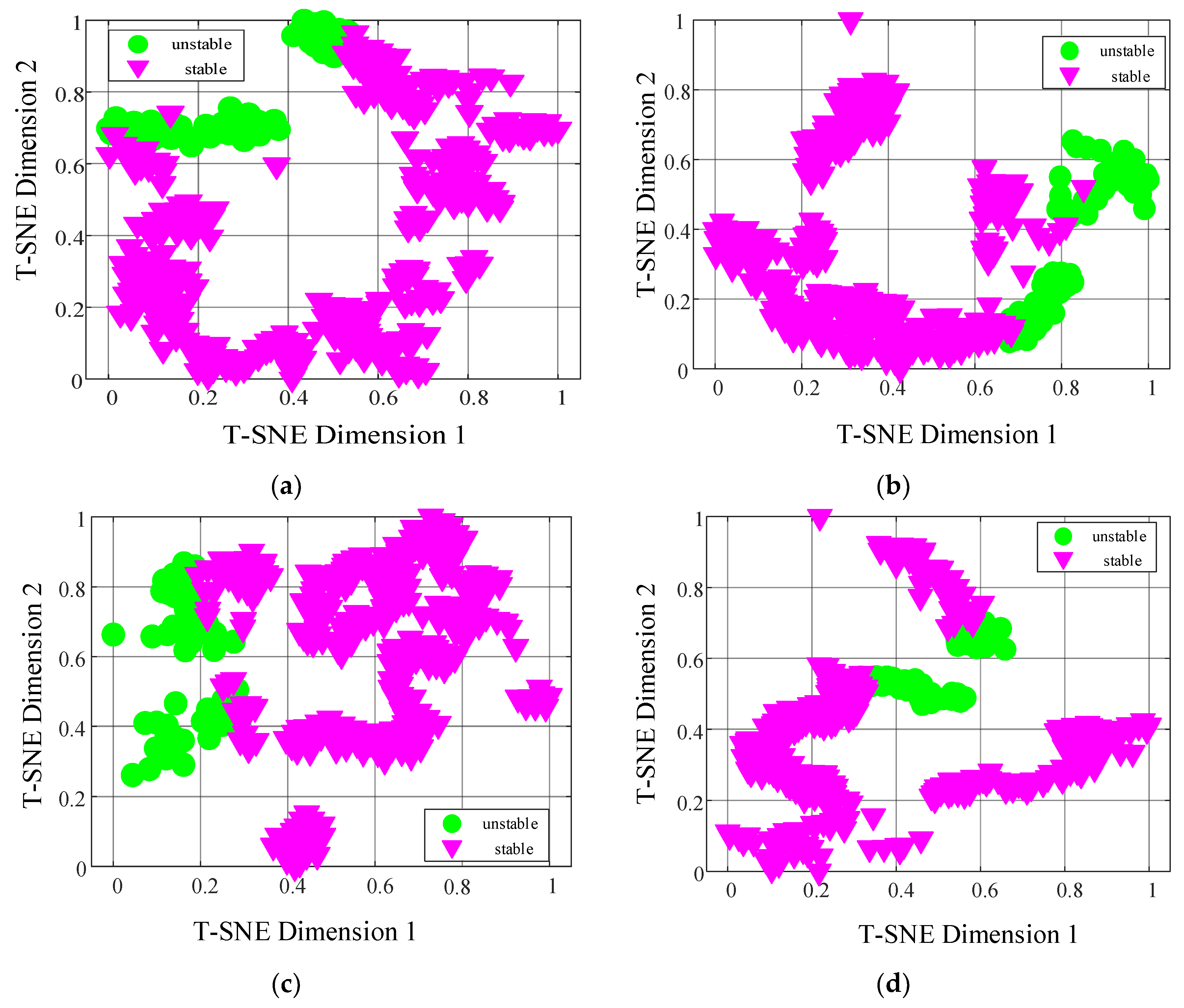
To visualize the results more clearly, the T-SNE algorithm was applied to reduce the dimensionality of the data. This visualizes the evolution of feature distributions across different residual blocks in CWT-ResNet. The extracted features are shown in Figure 15. In the original input features (Figure 16a), stable and unstable samples are highly overlapping and difficult to distinguish. The first residual block output (Figure 16b) begins to show preliminary separation, though with blurred boundaries. The distribution in the second residual block output (Figure 16c) gradually becomes clearer, with increased separation between categories. Finally, at the output layer (Figure 16d), the two sample types are completely separated, forming linearly separable distributions. As the network deepens, the distributions of different sample categories in the feature space progressively separate, while samples of the same category tend to cluster together, with their mutual distances significantly decreasing. The model gradually develops a clear ability to distinguish between stable and unstable samples, achieving linear separability in the feature space. This demonstrates that ResNet can effectively address the issue of inaccurate evaluation results, accurately identify the similarities and differences between samples in transient voltage responses, and possesses outstanding feature learning capabilities.

Figure 15. Feature results from the Stack-block1-conv1 layer.

Figure 16. Feature visualization results. (a) Original input data features. (b) Features from the first residual block output. (c) Features from the second residual block output. (d) Feature data from the model’s output layer.

4.5. Noise Resistance Analysis

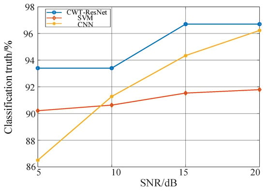
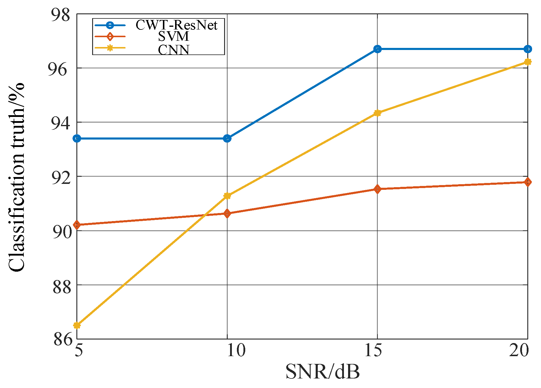
Due to factors such as weather conditions in the arid and desert regions of Northwest China, significant noise interference occurs during the evaluation process. To simulate real-world scenarios, noise levels of 5 dB, 10 dB, 15 dB, and 20 dB were applied to analyze the model’s robustness. Figure 17 shows classification accuracy under varying noise levels. The results indicate that even with deteriorated signal-to-noise ratio (SNR of 5 dB), CWT-ResNet maintains over 90% accuracy, while SVM and CNN accuracy drops to 91.27% and 86.57%, respectively. The residual structure of CWT-ResNet enhances the model’s tolerance to noise, demonstrating that the proposed method effectively suppresses noise interference. This also validates its strong adaptability to field monitoring data in practical engineering applications.

Figure 17. Noise resistance analysis results.

4.6. Adaptability Analysis

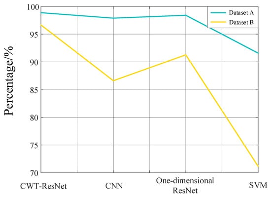
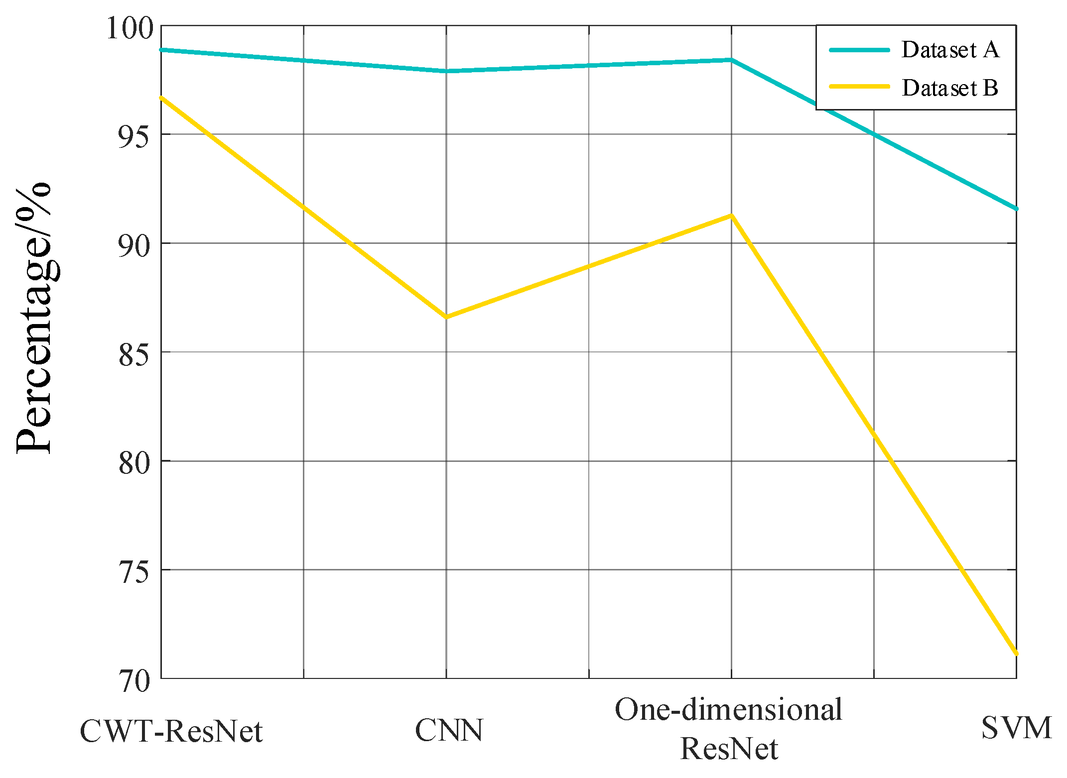
To validate the applicability of the proposed transient voltage stability assessment method, the model was tested on the DC blackout dataset (i.e., Dataset B), with results shown in Figure 18.

Figure 18. Adaptability analysis results.

As shown in the Figure 18, CWT-ResNet demonstrates significant advantages on both datasets, achieving an accuracy rate close to 97% with a relatively smooth curve. This indicates that the model possesses strong generalization capabilities and stability. In summary, the results in Figure 18 validate the superiority of CWT-ResNet in transient voltage stability assessment. It not only excels on standard datasets but also demonstrates excellent adaptability and robustness in real-world engineering data. This holds significant application value for voltage stability monitoring and early warning in complex scenarios such as new energy bases.

5. Conclusions

This paper addresses the challenges of feature extraction and sample class imbalance in large-scale renewable energy base DC transmission scenarios by proposing a transient voltage assessment method (CWT-ResNet) that integrates continuous wavelet transform with deep residual networks. Through simulation, the following conclusions are drawn:

(1)

Converting voltage time-series signals into two-dimensional time–frequency images via CWT effectively captures local dynamic features and frequency evolution patterns of non-stationary signals.

(2)

The deep residual network based on ResNet-50 automatically extracts high-order abstract features through stacked convolutional layers and residual modules, mitigating the vanishing gradient problem. The introduction of an improved focal loss function (FL) further enhances the identification capability of unstable operating conditions. The proposed method achieved an accuracy of 98.88% in computational examples, surpassing traditional models such as SVM and CNN by 7.31% and 3.11%, respectively.

(3)

Compared to traditional deep learning models, the proposed model maintains higher prediction accuracy under noisy conditions, demonstrating greater robustness. It also exhibits better adaptability across different fault scenarios.

The proposed method offers valuable insights for real-time monitoring and safe, stable operation of large-scale renewable energy bases such as desert and grassland wind farms.

References

- Liu, X.Y.; Shan, Y.P.; Xin, H.H.; Zheng, D. Transient voltage stability analysis of new energy grid-connected systems based on DC voltage control. Trans. China Electrotech. Soc. 2026, 1–13. [Google Scholar]
- Rao, H.; Zhang, D.H.; Zhao, X.B.; Guo, Q. Practice and analysis of UHV DC power transmission. High Volt. Eng. 2015, 41, 2481–2488. [Google Scholar]
- Ma, F.T. Discussion on the current status of UHV DC transmission technology and its application prospects in China. Electr. Power Equip. Manag. 2021, 43–44+65. [Google Scholar]
- Wang, H.; Liu, S.; Bian, J.; Li, G.Q.; Guo, J.Z.; Fu, Y.M. Rapid identification method of commutation failure risk areas in HC-HVDC systems under single-phase faults. Int. J. Electr. Power Energy Syst. 2026, 174, 111493. [Google Scholar] [CrossRef] [Scilit]
- Liu, X.Y. Transient Voltage Security Stability Analysis and Control of DC Sending-End Power Grids with High Proportion of New Energy. Ph.D. Dissertation, Zhejiang University, Hangzhou, China, 2024. [Google Scholar]
- Wu, L.; Chao, P.P.; Li, W.X.; Li, Z.M. A risk assessment method of multi-form transient voltage stabilities for high-proportion renewable energy sending-end power grids. Int. J. Electr. Power Energy Syst. 2026, 174, 111503. [Google Scholar] [CrossRef] [Scilit]
- Meng, X.Y.; Liu, C.; Zhang, Y.C.; Tian, R.D.; Gao, S.; Chen, Y.H. Integrated qualitative-quantitative assessment of power system transient stability based on DASeq2Seq and improved branch potential energy method. Electr. Power Syst. Res. 2026, 254, 112555. [Google Scholar] [CrossRef] [Scilit]
- Saberi, H.; Amraee, T.; Zhang, C.; Dong, Z.Y. A Benders-decomposition-based transient-stability-constrained unit scheduling model utilizing cutset energy function method. Int. J. Electr. Power Energy Syst. 2021, 124, 106338. [Google Scholar] [CrossRef] [Scilit]
- Hou, J.L.; Liu, Y.Q.; Xie, X.R.; Ye, M.; Sun, Y.X.; Wang, K.; Zhang, Y. A quantitative index and method for transient voltage stability assessment. Electr. Power Autom. Equip. 2015, 35, 151–156. [Google Scholar]
- Han, S.Z. A review of transient voltage stability assessment methods. Electr. Eng. 2023, 166–170. [Google Scholar] [CrossRef]
- Hou, Y.F.; Xu, T.Q.; Li, Y.; Zhu, M.M.; He, Z.L. Data-driven transient stability assessment of power systems with renewable energy integration and FACTS-based control strategies. Int. J. Electr. Power Energy Syst. 2025, 172, 111253. [Google Scholar] [CrossRef] [Scilit]
- Boričić, A.; Popov, M. Voltage vulnerability curves: Data-driven dynamic security assessment of voltage stability and system strength in modern power systems. Int. J. Electr. Power Energy Syst. 2025, 168, 110636. [Google Scholar] [CrossRef] [Scilit]
- Lashgari, M.; Shahrtash, S.M. Fast online decision tree-based scheme for predicting transient and short-term voltage stability status and determining driving force of instability. Int. J. Electr. Power Energy Syst. 2022, 137, 107738. [Google Scholar] [CrossRef] [Scilit]
- Zhou, Y.Z.; Wu, J.Y.; Ji, L.Y.; Yu, Z.H.; Lin, K.J.; Hao, L.L. Transient stability preventive control of power systems using chaotic particle swarm optimization combined with two-stage support vector machine. Electr. Power Syst. Res. 2018, 155, 111–120. [Google Scholar] [CrossRef] [Scilit]
- Satpathy, A.; Nayak, N.; Hannon, N.; Ali, N.H.N. A new real-time maximum power point tracking scheme for PV-based microgrid stability using online deep ridge extreme learning machine algorithm. Results Eng. 2023, 20, 101590. [Google Scholar] [CrossRef] [Scilit]
- Liu, M.S.; Sun, Z.Y.; Li, J.Z.; Zheng, K. Transient voltage fuzzy control method for receiving-end power grids based on convolutional neural networks. J. Harbin Univ. Sci. Technol. 2026, 1–11. [Google Scholar]
- Zhao, D.M.; Wang, Y. Transient voltage stability assessment of new energy bases based on CBAM-CNN-BiLSTM. J. N. China Electr. Power Univ. 2026, 1–11. [Google Scholar]
- Dong, J.Y.; Liang, J.F.; Wang, L.B.; Wang, Z.Z.; Gao, B.F. Improved transient voltage stability assessment method for DC receiving-end systems based on LSTM. J. Electr. Eng. 2026, 1–12. [Google Scholar]
- Liu, H.R.; Ren, H.; Zheng, Z.B.; Wang, W.; Xia, J.; Yang, J.H. Transient voltage stability assessment of power systems based on improved deep residual networks. Mod. Power 2023, 40, 879–889. [Google Scholar]
- Liu, S.K.; Dang, X.; Cui, Z.Q.; Yang, C.; Ruan, Z.H.; Yuan, M.Y. Transient stability assessment method for power systems based on deep residual networks for imbalanced samples. Smart Power 2024, 52, 116–123. [Google Scholar]
- Li, J.M.; Yang, H.Y.; Yan, L.P.; Liu, D.W.; Li, Z.H.; Xia, Y.Q.; Zhao, Y. Integrated evaluation method for transient stability of power systems with unbalanced samples. Autom. Electr. Power Syst. 2021, 45, 34–41. [Google Scholar]
Disclaimer/Publisher’s Note: The statements, opinions and data contained in all publications are solely those of the individual author(s) and contributor(s) and not of MDPI and/or the editor(s). MDPI and/or the editor(s) disclaim responsibility for any injury to people or property resulting from any ideas, methods, instructions or products referred to in the content. |
© 2026 by the authors. Licensee MDPI, Basel, Switzerland. This article is an open access article distributed under the terms and conditions of the Creative Commons Attribution (CC BY) license.