


Abstract
Accurate short-term photovoltaic (PV) power forecasting is crucial for maintaining grid stability. However, existing hybrid deep learning models suffer from inherent limitations owing to static feature-weighting mechanisms, often displaying significant phase lag and peak clipping under severe meteorological fluctuations. To address this, in this study, we adopt a hybrid CNN–LSTM–Attention forecasting framework incorporating an SE-based attention strategy. Field validation at a 150 kW PV power plant in Ningxia, China, demonstrated that the adopted model achieved a Root Mean Square Error (RMSE) convergence of 2.157 kW. Notably, this represented a 41.92% reduction in error compared to the standard LSTM benchmark and a further 16.46% improvement over the suboptimal CNN-LSTM baseline, explicitly confirming the specific contribution of the SE-based attention mechanism. Moreover, multi-weather evaluations and ablation studies confirm the framework’s robustness. Dynamic Time Warping (DTW) and Diebold–Mariano (DM) tests establish its statistical superiority and the reduction in phase lag against baselines. Residual analysis reveals a leptokurtic distribution with white noise properties, confirming the reduction in systematic bias. Consequently, this high-fidelity tracking allows precise minute-level ramping detection and decreases spinning reserve demands in practical power dispatch.
1. Introduction
The global energy transition relies heavily on solar photovoltaic (PV) generation, which provides electricity via clean distributed power systems [1]. Driven by carbon neutrality and fossil fuel reduction targets, the rapid growth of PV installed capacity over the last decade has transformed this energy source from a supplementary role to a primary electricity supply [2].
Unlike traditional thermal power plants, photovoltaic (PV) generation systems produce highly stochastic power that is strongly dependent on weather conditions [3]. The PV output power exhibits strong non-stationary oscillatory behavior because of three main factors, including sudden changes in solar irradiance, cloud movement paths, and nonlinear temperature fluctuations. The growing number of grid-connected PV systems creates major problems for electricity system stability because they produce large power variations that affect both supply and demand, system frequency, and power quality [4,5].
This is particularly evident in the Ningxia Hui Autonomous Region, China’s first comprehensive new energy demonstration zone. With a high density and proportion of PV installations, it shoulders the critical strategic function of the “West-to-East Power Transmission” initiative [6]. The region experiences a temperate continental climate that produces unstable and difficult-to-predict weather conditions. Local cloud movements and frequent sandstorms cause rapid and erratic fluctuations in PV power generation. The Ningxia grid faces significant challenges due to the high geographic concentration of PV systems, coupled with low local power consumption and strict transmission line safety limits [7].
Grid dispatchers must rely on expensive spinning reserve capacity for risk management due to the lack of highly accurate forecasting systems [8,9]. High PV integration can compromise grid stability, leading to unexpected power curtailment and system shutdowns during critical operational periods. Therefore, developing a highly accurate and robust short-term PV power forecasting model tailored to the meteorological and load characteristics of Ningxia is a prerequisite for ensuring the safe and stable operation of high-penetration renewable energy grids and enhancing regional energy efficiency [10].
The photovoltaic power forecasting paradigm has evolved from physical modeling and statistical learning to deep learning. Early physical models were based on photovoltaic principles and numerical weather prediction (NWP) [11]. Early physical models were based on photovoltaic principles and numerical weather prediction (NWP). Recently, the physical modeling landscape has expanded from traditional system-level estimations to advanced device-level and multi-scale simulations. For instance, detailed simulation frameworks for emerging photovoltaic technologies, such as perovskite solar cells, have provided deeper insights into device physics and theoretical performance limits [12]. Despite these advancements in physical and device-level modeling, their application in real-time grid forecasting remains challenging. Their accuracy is highly sensitive to physical parameters, and they struggle to capture rapid transient meteorological changes. Subsequently, data-driven methods such as SVR and BPNN have demonstrated effectiveness for stationary sequences [13]. However, these shallow models lack a memory mechanism, rendering them ineffective for modeling long-term dependencies. This limitation results in a significant phase lag during high-frequency fluctuations, such as cloud shading, and fails to meet real-time scheduling demands.
LSTMs with gating mechanisms have emerged as a mainstream approach for addressing these limitations. They effectively overcome the vanishing gradient problem and capture temporal evolution patterns, demonstrating superior performance compared to ARIMA and SVR [14]. However, although standalone LSTMs excel at capturing longitudinal temporal dependencies, they exhibit deficiencies in handling the lateral spatial coupling of multidimensional meteorological factors. Owing to the lack of explicit extraction of local spatial correlations [15], these models tend to output smoothed trends, leading to a peak-shaving phenomenon under high-frequency fluctuations and loss of signal texture.
To address this spatial perception gap, a CNN-LSTM spatiotemporal parallel paradigm was adopted. In this architecture, CNNs serve as feature extractors to capture local patterns, whereas LSTMs handle temporal modeling [16], effectively filtering background noise and enhancing the capture of high-frequency fluctuations. Despite their improved accuracy, existing hybrid models are constrained by static feature-weighting mechanisms. Standard architectures treat all input channels equally and lack mechanisms to dynamically recalibrate weights based on real-time environmental factors (e.g., cloud opacity dominance during overcast conditions). This lack of adaptive attention causes sluggish model responses, thereby inducing prediction bias and phase lag [17].
The recent literature [18] typically integrates temporal attention mechanisms into standard CNN-LSTM networks; however, when handling multidimensional inputs, these approaches often assign identical channel attention weights to all meteorological variables. This method has limitations when dealing with localized transient noise (such as the sudden gusts characteristic of the Ningxia region). Furthermore, existing work primarily focuses on deterministic point forecasts and lacks quantitative analysis of temporal alignment errors. To address these issues, the CNN–LSTM–Attention architecture in this paper introduces a channel-level recalibration mechanism to dynamically suppress specific noisy meteorological features.
Existing hybrid models often treat meteorological inputs with static weights and fail to adapt to regime shifts between stable clear sky and volatile cloudy weather conditions [19]. While recent studies have explored combinations of CNN, LSTM, and standard attention mechanisms for time-series forecasting, most treat the attention module as a generic mathematical feature selector. These existing works primarily focus on general power grid environments with stable climatic variations. In contrast, our approach directly targets the distinct and severe meteorological challenges of the Ningxia region, which is characterized by temperate continental extremes, frequent localized sandstorms, and rapid irradiance shifts. Instead of applying a generic attention layer, we configure the Squeeze-and-Excitation (SE) bottleneck specifically to act as an environment-aware adaptive filter. This design ensures the network autonomously suppresses background sensor noise during stable clear sky periods and rapidly increases sensitivity to critical weather transition factors, such as sudden cloud opacity changes. The main contributions of this study are as follows:
1. Construction of a deeply coupled spatiotemporal feature architecture: A cascaded convolutional neural network–long short-term memory (CNN-LSTM) structure was adopted in which the convolutional neural network extracts multidimensional local spatial features while filtering background noise, thereby resolving the “zero-value drift” issue. When combined with the long short-term memory network, which captures long-term temporal dependencies, this architecture significantly enhances the model’s dynamic tracking capability for nonlinear fluctuations.
2. Integration of the environment-aware SE-based attention strategy: This approach overcomes the inherent static weight bottleneck of conventional methods by integrating the self-attention (SE) module to construct adaptive filters. This mechanism dynamically adjusts feature weights based on real-time meteorological conditions (e.g., enhancing responsiveness to cloud transparency) and reduces prediction biases caused by weight allocation delays.
3. Multidimensional empirical validation and mechanism analysis: Using real-world data from a 150 kW power station in Ningxia, ablation experiments demonstrated that the SE-based attention mechanism reduced the Root Mean Square Error by an additional 16.46% under cloudy conditions. Combined with the micro-error distribution and residual time-series analysis, this quantitatively proves the exceptional robustness of the model in reducing the phase lag and achieving statistical unbiasedness.
2. Methodology
2.1. Model Framework
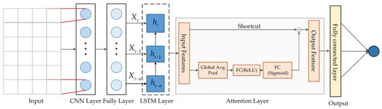
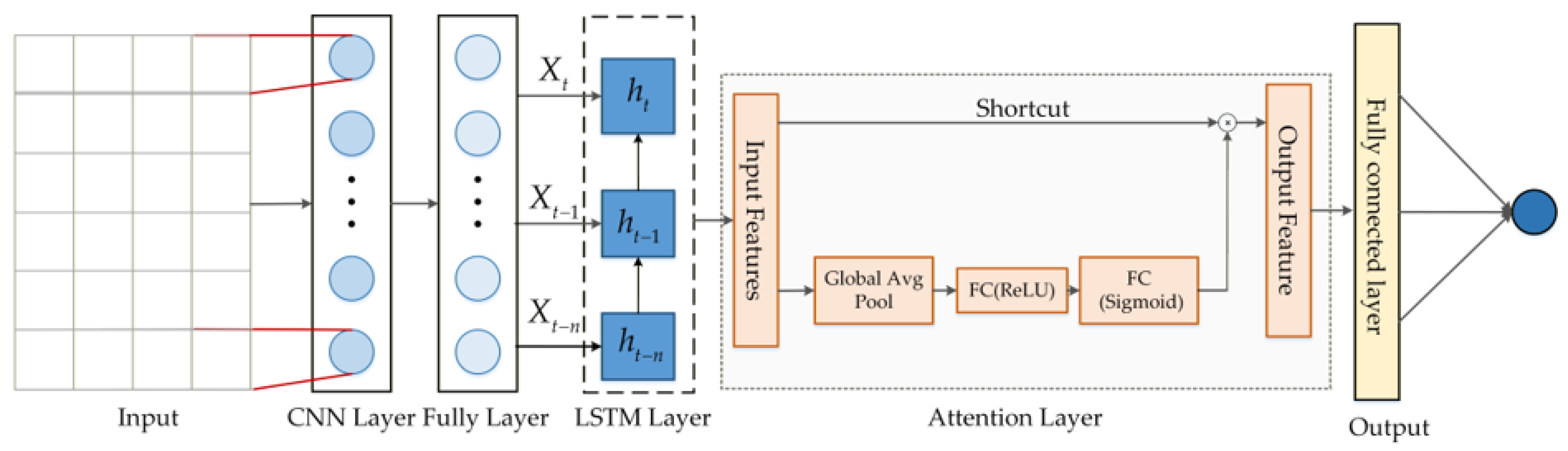
This study developed a hybrid prediction system that combines a CNN with an LSTM and attention mechanisms (Figure 1) to perform predictions through three sequential stages.
Figure 1.
Architecture of the CNN–LSTM–Attention framework. The diagram illustrates the integrated structural design of the forecasting model. The input data is processed through the CNN layer for spatial feature extraction, followed by the LSTM layer for temporal modeling. The attention layer, featuring a shortcut connection and global pooling, operates to adjust the weight of feature channels before reaching the final output layer.
1. Spatial Feature Extraction (CNN): A 1D convolutional neural network functions as the front-end encoder and extracts spatial relationships and local patterns from the seven-dimensional meteorological data. This process transforms complex data features into simpler forms that remove high-frequency sensor jitter noise [20].
2. Temporal Feature Learning (LSTM): This stage analyzes the output features from the CNN to detect both short- and long-term dependencies, as well as nonlinear temporal patterns in the PV power data.
3. The SE-based attention mechanism embedded in our model allows it to perform adaptive weight allocation. The system amplifies dominant factors based on real-time meteorological data and suppresses background noise, passing refined features to a fully connected layer to generate final predictions.
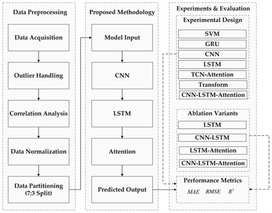
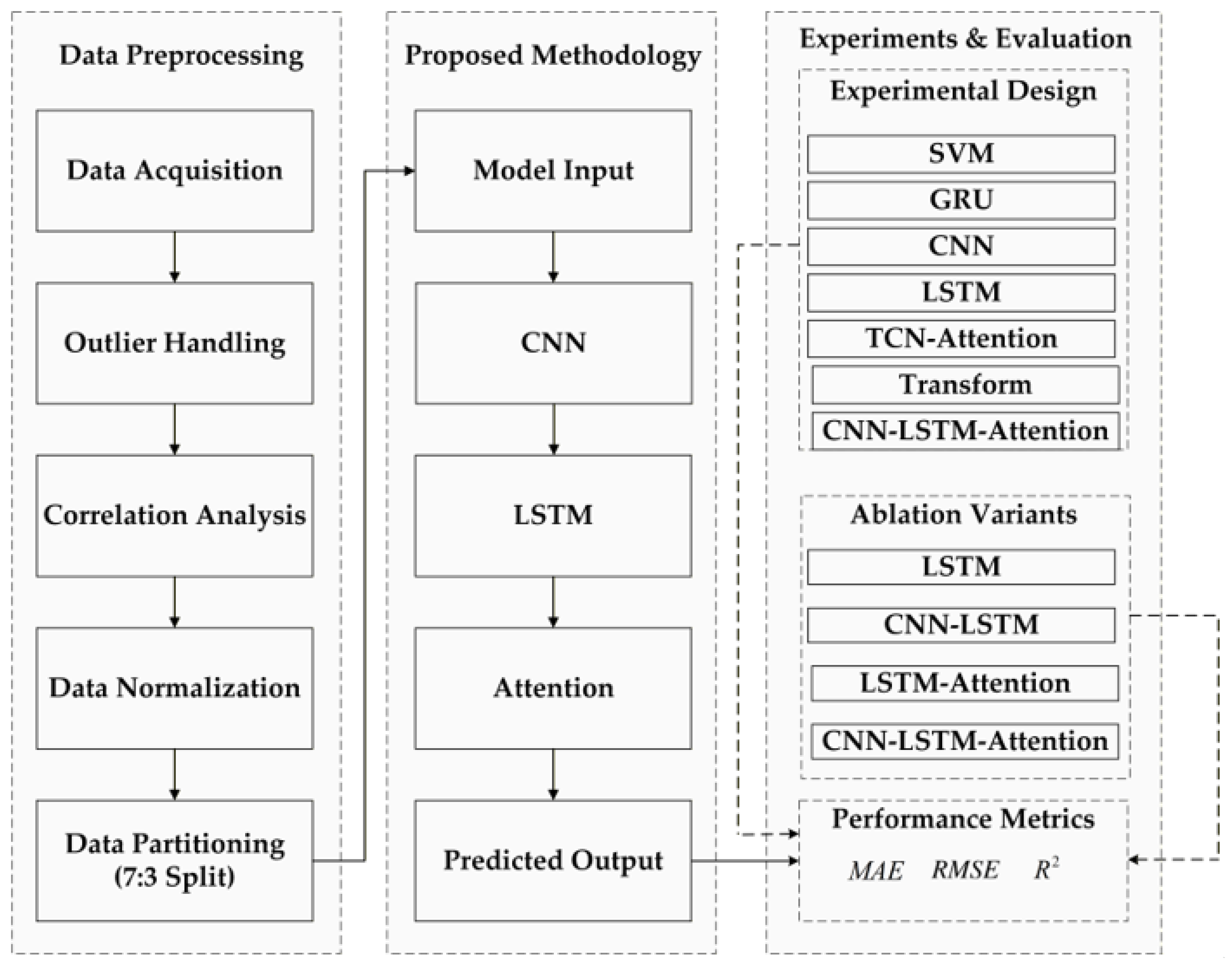
The flowchart in Figure 2 shows the entire technical method of this study through its three stages, which follow each other in order.
Figure 2.
Flowchart of the CNN–LSTM–Attention forecasting methodology. The diagram outlines the research framework across three modules: data preprocessing, the proposed methodology, and experimental evaluation. It details the sequential steps from data acquisition and model construction to the final calculation of performance metrics.
The data preprocessing module implements a standardized workflow that begins with data acquisition, continues with outlier handling and correlation analysis, and ends with normalization operations. Subsequently, the dataset was split into training and testing sets at a ratio of 7:3. The method module develops a hybrid system that unites convolutional neural networks (CNNs) with long short-term memory (LSTM) and attention mechanisms. The system operates through three consecutive stages: spatial feature extraction, temporal evolution modeling, and SE-based attention calculation. The experiment and evaluation module contains two sections which compare benchmark models including support vector machines and recurrent neural networks and perform ablation studies to measure prediction accuracy through multiple performance indicators such as , , and .
2.2. Spatial Feature Extraction Module
This study deploys a 1D-CNN as the front-end feature encoder, aiming to extract local robust features from high-dimensional multivariate inputs while suppressing high-frequency noise [21]. Given an input matrix (), the model configures 32 convolutional kernels (size ) to perform one-dimensional convolution operations:
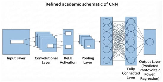
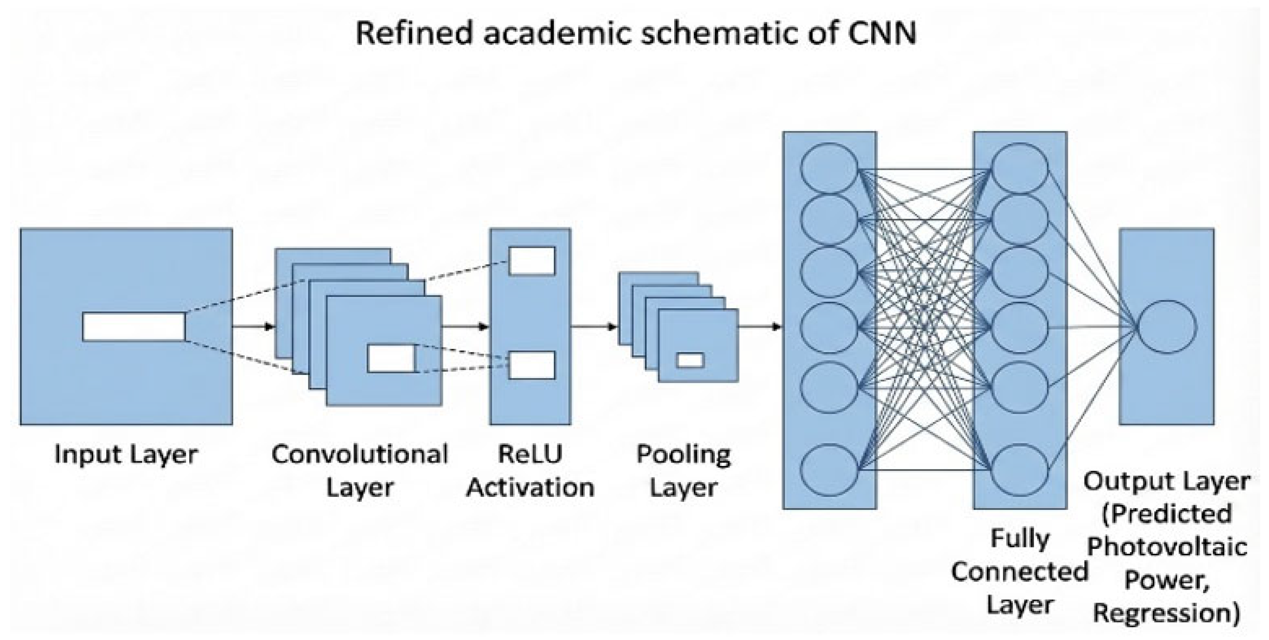
The feature vector reconstructed through convolution explicitly captures spatial coupling relationships among meteorological factors. This approach reduces computational complexity while significantly enhancing the model’s sensitivity to abrupt signals such as instantaneous cloud occlusion, as illustrated in Figure 3, depicting the CNN schematic.
Figure 3.
CNN principle diagram. The schematic illustrates the convolution and pooling operations for spatial feature extraction. The structure shows the transformation of input data into feature maps.
2.3. Temporal Feature Learning Stage
Following the reconstruction of spatial features by the front-end CNN, this stage employs an LSTM to construct a temporal model. This approach addresses the historical inertia of PV power and the inability of traditional RNNs to capture long-term sequence dependencies due to vanishing gradients [22].
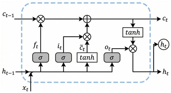
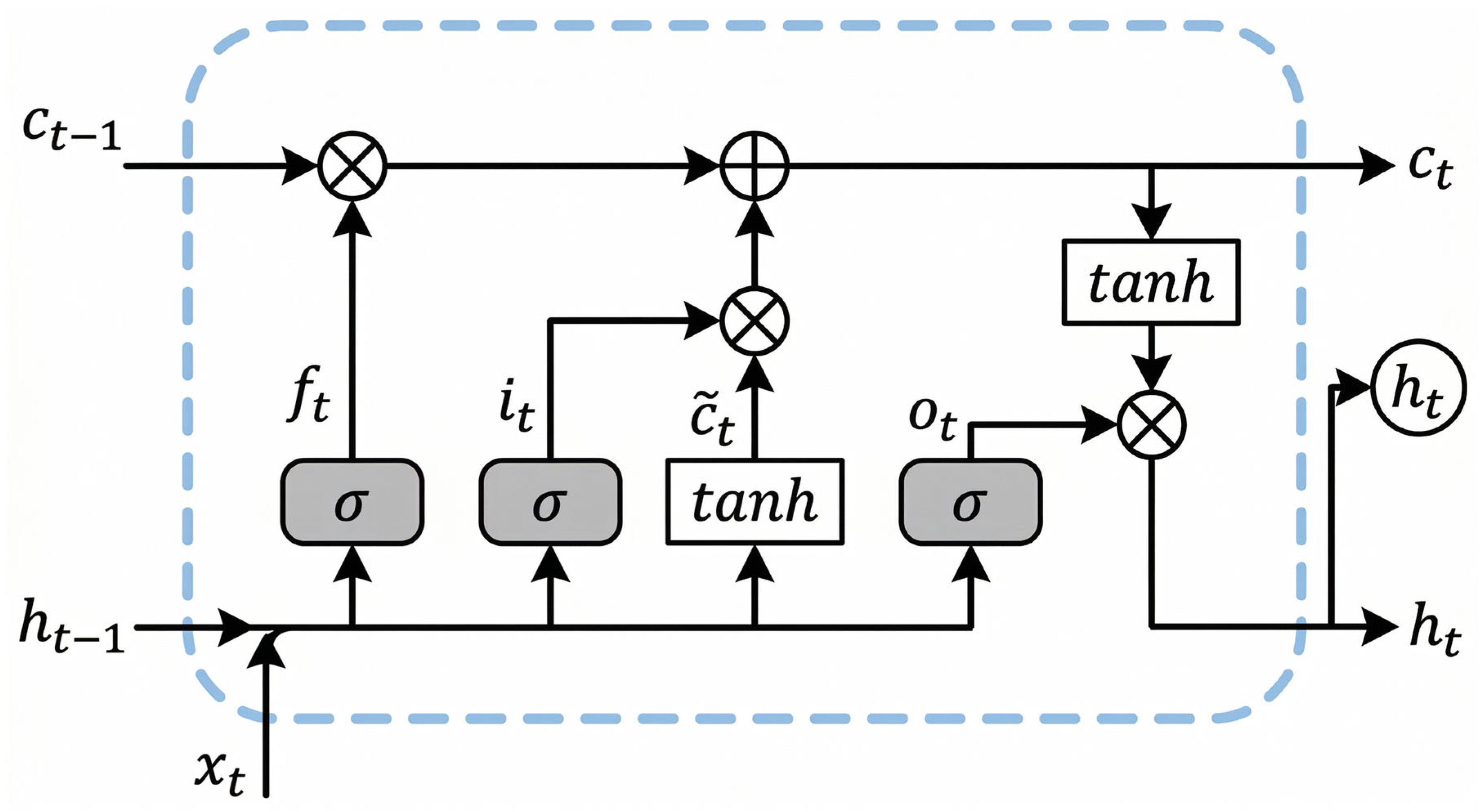
The core of the LSTM lies in its gating mechanism, which regulates the flow of information through memory and forgetting operations. State updates at time follow this logic:
Forget gate : Filters the previous cell state via a Sigmoid function to reduce redundant historical features:
Input gate : Evaluates the input in conjunction with the candidate state to determine the incorporation of new features:
State update : Utilizes the Hadamard product to fuse historical retention with newly acquired information, enabling long-term memory:
Output gate : Generates the hidden layer output via nonlinear mapping based on , completing the temporal deep encoding:
where denotes the CNN feature components; represents the previous hidden state; and denote the weight matrices and bias vectors, respectively; denotes the Sigmoid activation function; and denotes element-wise multiplication.
This study configured 64 hidden units to model nonlinear dynamics. The output sequence achieves deep coupling between the spatial features and temporal patterns, providing high-level semantic representations for the subsequent attention mechanism Figure 4 shows the LSTM schematic diagram.
Figure 4.
Schematic of the LSTM network structure. The diagram illustrates the internal configuration of the long short-term memory (LSTM) cell. It presents the gating mechanisms—comprising the forget, input, and output gates—which regulate the information flow within the cell state () and hidden state (). The symbolic representations of the pointwise operations and activation functions are also indicated.
2.4. Adaptive Weight Allocation Module
The Squeeze-and-Excitation (SE) block is integrated to address the volatile meteorological dynamics of the Ningxia region, which is characterized by high solar potential but abrupt weather fluctuations and dust interference. Unlike standard temporal attention, which assigns weights across entire time steps, the SE mechanism performs channel-wise recalibration to target feature-specific transient noise. By learning adaptive weights, the SE block dynamically suppresses noisy channels (e.g., wind anomalies) while prioritizing critical variables like solar irradiance. This targeted feature weighting improves prediction robustness against the rapid weather variations typical of this region.
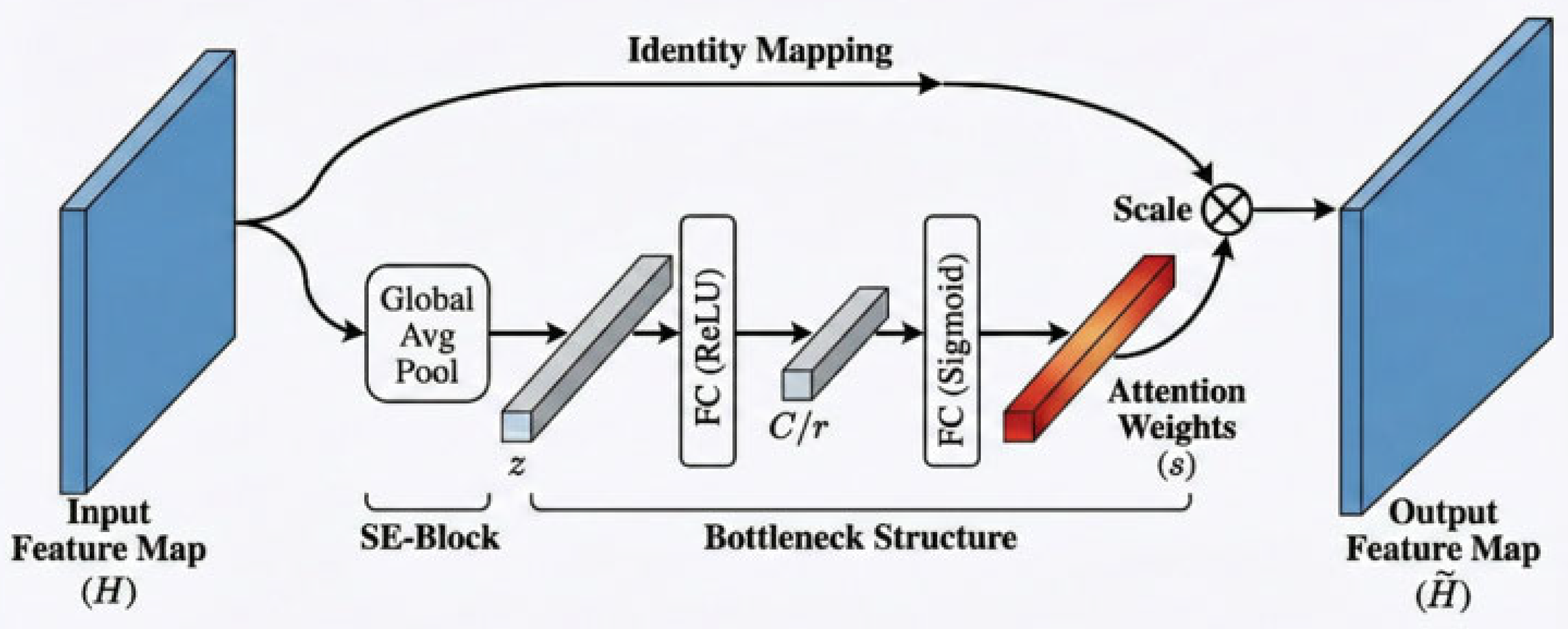
To address the limitation of static feature weights in CNN-LSTM architectures, which fail to adapt to non-stationary meteorological variations [21], an SE-based attention mechanism is embedded after the LSTM layer. This module explicitly models the nonlinear dependencies between channels through an SE-based attention strategy. Let the LSTM output feature be denoted as (where ). The computation process comprises three key steps:
Squeeze: Temporal features are aggregated into channel statistics via global average pooling:
Excitation: Channel weights
are learned using a bottleneck structure (comprising two fully connected layers with a dimensionality reduction ratio of
):
where and denote the ReLU and Sigmoid activation functions, respectively, and and represent the weight matrices.
Scale: The normalized weight is applied to the original feature to generate the rescaled feature :
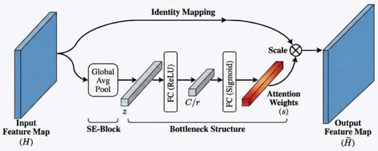
Unlike standard computer vision applications where SE blocks treat all spatial features uniformly, the dimensional reduction ratio in our bottleneck structure is specifically configured for high-frequency meteorological data. The physical implication of this design is that the network learns to dynamically switch its focus between macro-trends (driven by base temperature and irradiance) and micro-disturbances (driven by rapid wind speed variations or cloud cover). This architectural consideration directly addresses the temporal delay and peak-shaving commonly observed in conventional hybrid models when applied to the highly volatile Ningxia dataset. Figure 5 illustrates the principle of the SE-based attention mechanism.
Figure 5.
Mechanism of the SE-based attention module. The diagram illustrates the sequence of the channel-wise attention process. The input feature map is first processed through global average pooling to obtain channel-specific descriptors. A bottleneck structure then uses fully connected layers to calculate attention weights. These weights are applied to the original features to produce the output feature map.
2.5. Model Training Strategy
This study formulated photovoltaic power forecasting as a supervised regression problem.
Objective Function: The Mean Squared Error (MSE) is selected as the loss function to heavily penalize samples with large prediction errors, defined as follows:
where denotes the total number of samples, represents the ground truth (actual value), and is the predicted value generated by the model for the observation.
In this study, the forecasting model utilizes an input time window of 8 time steps. With a 15 min sampling frequency, this equates to a 2 h historical observation period. The model builds its input sequence from 7 feature variables recorded across these 8 consecutive intervals.
Optimization and Regularization: The Adam optimizer was employed to adaptively adjust the learning rate. Utilizing the MATLAB Deep Learning Toolbox, a dual regularization strategy is implemented: learning rate decay is introduced to suppress oscillations near the optimal solution, and gradient clipping is applied to mitigate the risk of gradient explosion within the deep LSTM networks, as shown in Table 1. The core parameters of all CNN layers are listed separately in Table 2.
Table 1.
The specific model hyperparameter settings are detailed.
Table 2.
CNN layer parameter settings.
To ensure a fair comparison, the exact same hyperparameter tuning methodology and data partitioning (identical training and testing sets) were applied to both the model and all benchmark models. For every model, standard components (e.g., the Adam solver, ReLU activation functions, and a gradient threshold of 1) were kept constant.
For model-specific critical variables, a targeted grid search evaluated combinations within predefined search spaces.This standardized approach ensures that all baselines were pushed to their maximum predictive capability under identical conditions before comparison.
3. Experimental Setup and Data Processing
3.1. Data Description
This experiment utilized real-world data from a 150 kW photovoltaic power station in Ningxia. The dataset contained complete 2019 data, providing 15 min spatiotemporal observations throughout the entire year. The climate in Ningxia maintains stable conditions throughout time, and the 2019 dataset includes all major extreme weather occurrences, including sandstorms, making it an appropriate benchmark for testing model stability. The research excluded zero-value nighttime data and focused the analysis on the effective generation window from 06:00 to 20:00 for each valid operational day. The dataset contained photovoltaic power generation as the target variable, along with seven meteorological characteristics: irradiance, temperature, wind speed, wind direction, cloud opacity, relative humidity, air pressure, and actual power. The total number of samples was 21,900 after completing all preprocessing steps. The chronological time-series data were split into a 70% training set and a 30% testing set. Table 3 lists all features and units.
Table 3.
Unit of influencing factors.
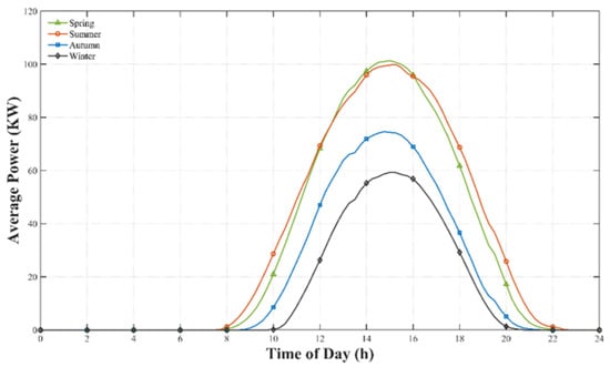
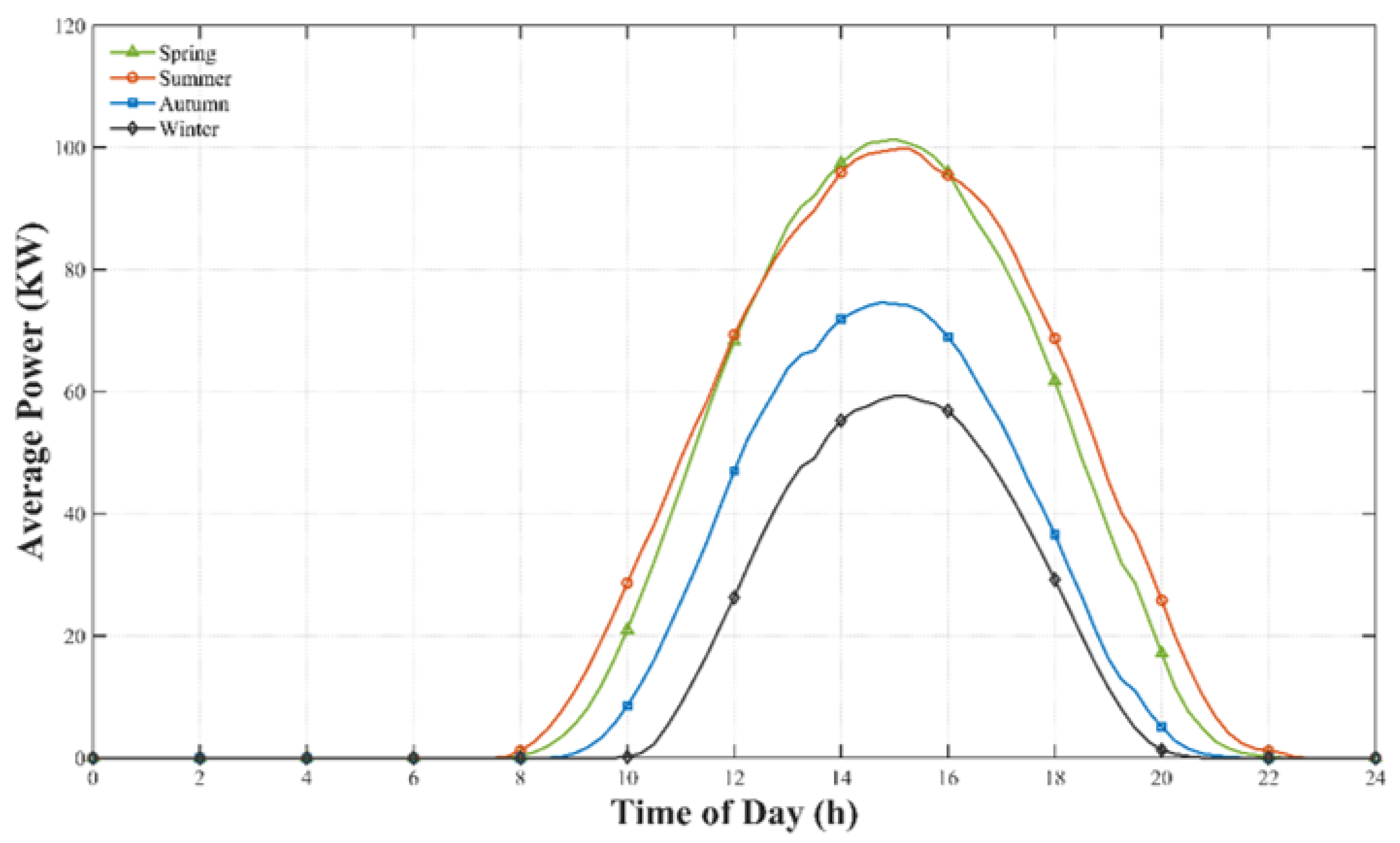
To elucidate the temporal distribution characteristics of photovoltaic power under different climatic conditions, this study divided the annual dataset of a photovoltaic power station in Ningxia into four seasonal subsets. Figure 6 shows the calculated average daily power curve, which effectively smooths out random meteorological fluctuations and highlights the inherent seasonal trends.
Figure 6.
Seasonal PV power profiles. The graph presents the diurnal variation in average photovoltaic power output across the four seasons. The curves illustrate the shifts in peak generation and solar window duration among spring, summer, autumn, and winter.
The power generation characteristics become evident through the analysis of these curves. Summer (orange line) operates with the largest effective power generation window, which spans from 06:00 to 20:00 because of the highest solar altitude angle. Conversely, winter (black line) presents the most constrained generation profile, with significant reductions in both the operational time span and peak power output. Notably, the peak power in summer is not significantly higher than that in spring (green line), displaying a phenomenon known as “peak parity.” This phenomenon occurs because springtime clear skies and minimal aerosol particles maximize sunlight penetration, whereas summer monsoon clouds increase atmospheric opacity. The thermal degradation effect, which occurs when ambient temperatures reach high levels, leads to decreased module conversion efficiency, which results in reduced actual radiation benefits from longer daylight periods. The model shows excellent generalization abilities because it successfully predicts all seasonal data patterns.
3.2. Feature Correlation Analysis
The Pearson correlation coefficient (PCC) was used for statistical analysis to assess the linear correlation between the input meteorological factors and solar output power [23], as well as to prove feature selection. For variables and , the correlation coefficient is calculated as follows:
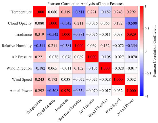
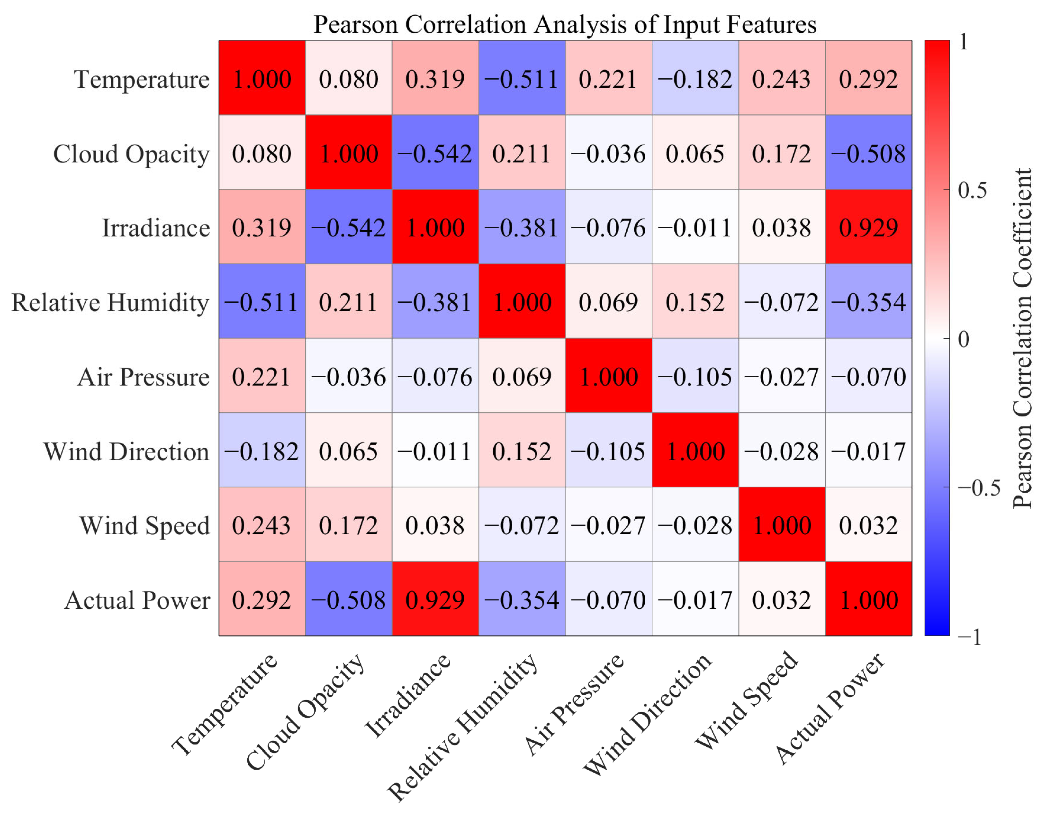
where denotes the total sample size, and and represent the mean values of the variables, respectively. The correlation coefficients between each input variable and output power are shown as a heatmap in Figure 7. The statistical analysis yielded the following results:
Figure 7.
Pearson correlation coefficient heatmap. The matrix illustrates the statistical dependencies between the input meteorological features and the actual PV power output. Each cell contains the correlation coefficient, with the color gradient indicating the degree of association between the variables.
A positive association exists, with a correlation coefficient of 0.929 between global irradiance and PV power, indicating it as the principal determining element. The module temperature has a correlation value of 0.292. This result suggests that increased irradiance results in greater module temperature, in accordance with thermodynamic principles.
A negative connection exists between cloud transmittance and relative humidity. These factors are correlated with values of −0.508 and −0.354, respectively, indicating a decrease in the effects of cloud cover and elevated humidity on solar radiation.
Such features with weak association are retained: The absolute values of the linear correlation coefficients for wind speed and wind direction are both below 0.100. This holds notwithstanding the small linear connection. Wind speed is preserved as a nonlinear feature input owing to its strong physical cooling effect on solar modules. Ultimately, this approach allows the deep learning architecture to identify intrinsic power fluctuation patterns among climatic variables instead of depending only on linear mapping [24].
In conclusion, all seven meteorological variables—temperature, cloud transparency, irradiance, relative humidity, air pressure, wind direction, and wind speed—were comprehensively included in the system. That supports the model’s input framework, grounded in their statistical features and physical value.
3.3. Data Preprocessing
Before inputting into the model for training, the raw photovoltaic dataset must undergo a strict preprocessing pipeline to ensure data integrity and algorithm stability. To meet the requirements of deep neural networks regarding input data distribution and to construct high-quality supervised learning samples, the specific standardized preprocessing steps are as follows:
1. Time Window Extraction: First, the effective time period of the dataset is limited to the active power generation period between 06:00 and 20:00. This temporal filtering directly removes the invalid intervals of zero power generation at night, effectively reducing the interference of non-informative data on the model.
2. Outlier Removal: A strict cleaning mechanism is implemented for abnormal data caused by reasons such as sensor failures. First, samples containing missing values (NaN) in the meteorological inputs or the target power vector that cannot be repaired are directly discarded. Second, statistical criteria are introduced to detect and exclude extreme outliers: any measurement data deviating from the mean of its respective feature by more than three standard deviations () is reduced.
3. Missing Value Imputation Strategy: When processing missing data, to maintain time-series continuity while strictly observing temporal causality (prohibiting the use of future data), this study adopts different imputation strategies for the training and testing sets:
Training Set (Historical Archived Data): Since the training phase uses historical data to learn global mapping rules, linear interpolation is applied to fill in short-term missing data (time spans 30 min [24]). This method allows the model to adapt to the natural variation patterns of meteorological data while avoiding the introduction of artificial step features into the data. The calculation formula is as follows:
Testing Set (Simulating Real-Time Operation): To simulate a realistic real-time forecasting environment (where future information is absolutely unavailable), a forward fill (Last Observation Carried Forward/LOCF) strategy is adopted. If data at time is missing due to sensor delay or failure, it is directly replaced with the most recent valid observation . This effectively prevents the problem of data leakage and strictly aligns with the actual operational constraints of the power grid dispatching system [25].
4. Data Normalization: Significant differences in dimensions and orders of magnitude exist among the raw meteorological data (for example, the numerical ranges of total irradiance and photovoltaic panel temperature differ greatly). To ensure the stability of the learning dynamics of the CNN–LSTM–Attention architecture and reduce scale differences among the 7 meteorological variables, this study introduces Min-Max Scaling. Both input features and target outputs are mapped to the interval using the following formula:
where
represents the original measurement value, and and correspond to the minimum and maximum values of the specific feature, respectively. Key Control Point: To strictly prevent data leakage, the calculation of and relies only on the training set data. The testing set data is subsequently scaled using the parameters determined from the training set, thereby ensuring the absolute reliability of the model evaluation.
3.4. Evaluation Metrics
To quantitatively assess the model’s predictive performance, three statistical metrics are employed: Root Mean Square Error (RMSE), Mean Absolute Error (MAE), and coefficient of determination ().
Root Mean Square Error (RMSE):
Mean Absolute Error (MAE):
where represents the number of test samples, is the actual value, and denotes the predicted value for the sample. Specifically, RMSE is sensitive to outliers due to the squaring operation, while MAE provides a more direct representation of the average error magnitude. A lower value for these metrics indicates superior model performance.
Coefficient of Determination ():
This represents the model’s goodness of fit to the variability in the observed data. The formula is as follows:
where is the total number of samples in the test set, is the actual observed power value of the sample, is the model’s predicted value, and is the arithmetic mean of the actual observed values.
3.5. Sensitivity Analysis and Training Stability
The prediction accuracy of deep neural networks relies heavily on structural and training parameters. To manage computational costs, variables were divided into empirically fixed settings and systematically tuned ones (Table 1). Standard components like the Adam optimizer, ReLU activation, and a gradient threshold of 1 were fixed based on deep learning conventions.
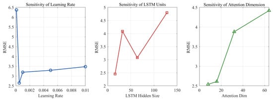
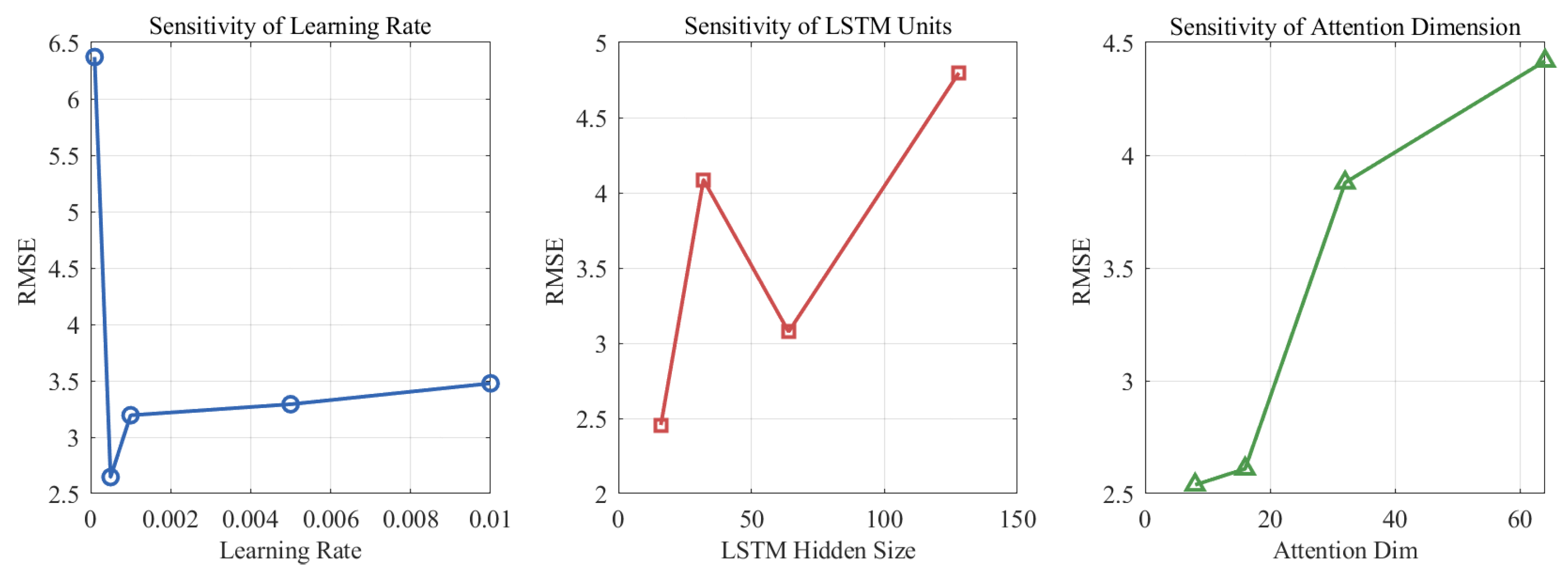
For critical variables, a targeted grid search evaluated combinations across defined search spaces: initial learning rate (0.0001 to 0.01), LSTM hidden units (16 to 128), attention reduction dimension (8 to 64), and mini-batch size. To detail the impact of these choices, a sensitivity analysis (Figure 8) assessed how varying individual parameters affected the RMSE while holding others constant.
Figure 8.
The impact of different hyperparameters on model prediction accuracy (RMSE) The three panels present the RMSE variations across different settings of the learning rate, LSTM hidden size, and attention dimension. The blue circle represents the learning rate; the red square represents the size of the LSTM; and the green triangle represents the attention dimension.
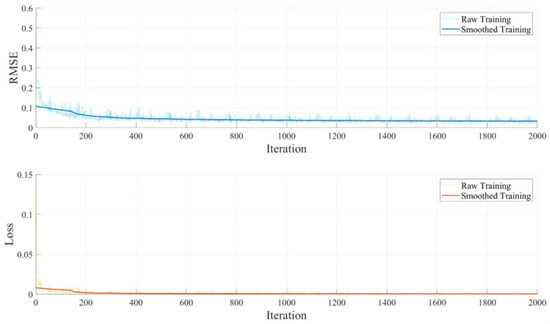
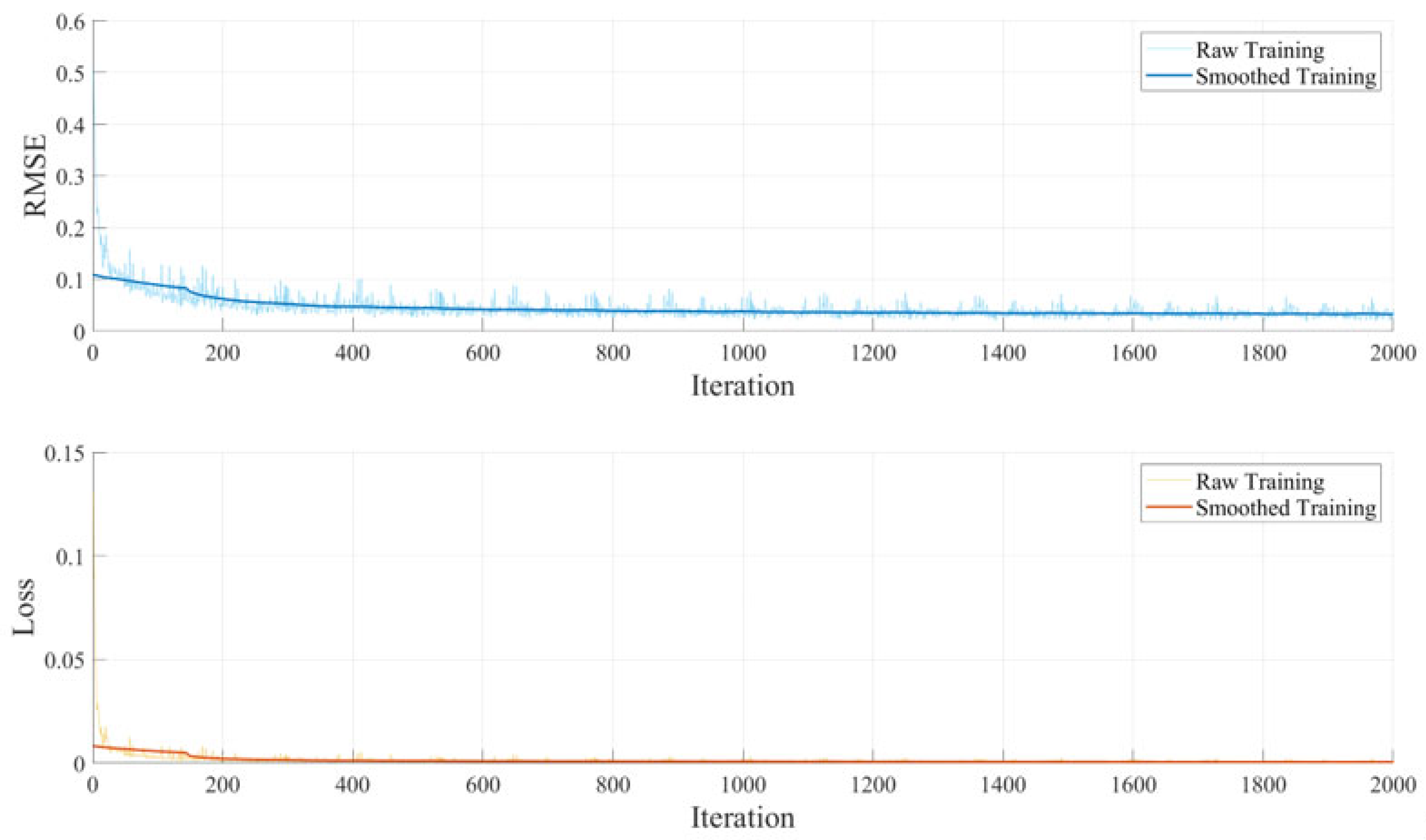
Although univariate tests showed that smaller individual parameters (e.g., 16 LSTM units or a 0.0005 learning rate) yielded localized minimum errors, deep neural networks feature strong parameter coupling. Combining all individual minimums restricted the network’s overall learning capacity. Consequently, joint testing confirmed that a 0.001 learning rate, 64 LSTM units, and an attention dimension of 32 achieved the lowest global error. This final configuration balances the structural capacity needed for complex weather data with accurate temporal filtering. Finally, Figure 9 verifies that the network reaches a steady state with these settings.
Figure 9.
Training process of the CNN–LSTM–Attention model. The graphs present the variation in RMSE (top) and loss (bottom) over 2000 iterations. Both panels include the raw training values and the corresponding smoothed curves to show the training progression.
3.6. Hyperparameter Configurations and Baseline Optimization
To establish a transparent assessment framework, the dataset is chronologically divided strictly into a training set (70%) and a testing set (30%). Furthermore, to maintain training stability and prevent the exploding gradient problem in recurrent architectures, gradient clipping is applied during the learning process.
As shown in Table 4, we have illustrated the parameter settings for all the basic models. Specifically, standard recurrent architectures (LSTM and GRU) achieved stable convergence with 20 hidden units and an initial learning rate of 0.001. However, for complex hybrid frameworks designed to capture the daily cyclical patterns and short-term fluctuations of power generation sequences, structural adjustments were necessary. For instance, the Transformer baseline was configured with restricted capacity (2 attention heads and an embedding dimension of 32) combined with a dropout rate of 0.2. This specific configuration was selected through extensive testing to effectively model spatial–temporal dependencies while actively preventing the severe overfitting often observed when applying large-scale attention mechanisms to this type of data. Regarding training dynamics, while most baselines utilized a standard batch size of 64, the Transformer required a reduced batch size of 32 to manage the higher memory demands of self-attention operations and preserve training stability. These carefully calibrated settings ensure that the final comparative analysis reflects the actual structural advantages of each method, rather than artifacts of mismatched training conditions.
Table 4.
Base model hyperparameters.
To provide a clear reference for the computational cost, all experiments were conducted on a workstation equipped with a 13th Gen Intel Core i7-13700H processor (Dell (China) Co., Ltd., Xiamen, China) (2.40 GHz) and 16.0 GB of RAM, running on a Windows 11 operating system. The deep learning models were implemented using the MATLAB 2024b environment. Under this hardware and software configuration, the training process for the adopted CNN–LSTM–Attention model took approximately 15 min per run to reach convergence. Documenting this baseline computational time provides an objective reference for future reproduction and application evaluations.
4. Results and Discussion
4.1. Analysis of Overall Prediction Performance
This study conducted a systematic benchmark comparison experiment to thoroughly assess the predictive performance and generalization limits of the CNN–LSTM–Attention architecture we adopted, including three primary types of mainstream methods. The benchmark models included conventional shallow machine learning (SVM), single-layer deep neural networks (CNN, LSTM, and GRU), basic hybrid architectures (CNN-LSTM), and recent mainstream deep learning architectures (Transformer and TCN-Attention).
While recent advanced models such as Informer, Autoformer, or PatchTST have shown strong capabilities in long-sequence time-series forecasting, they were not included in the current benchmark comparison. The primary reason is that these large-scale Transformer-based architectures typically require massive datasets to train effectively and prevent overfitting. Given the specific scale of our regional dataset, deploying such complex models would significantly increase computational costs with minimal guaranteed proportional accuracy gains for short-term predictions. Furthermore, the core objective of this study prioritizes engineering applicability, computational efficiency, and robust performance under complex meteorological fluctuations, rather than conducting a pure benchmark competition against the latest algorithmic architectures.
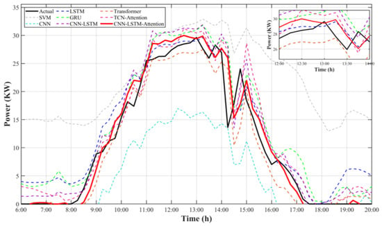
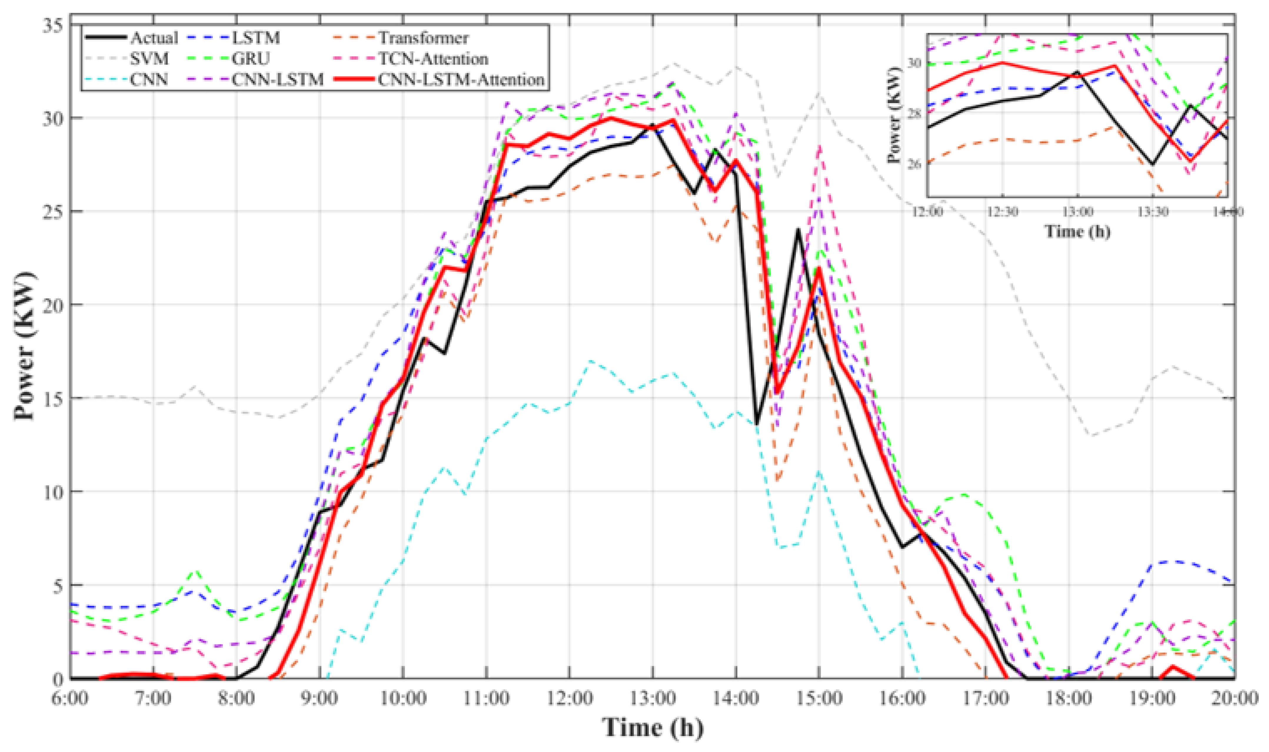
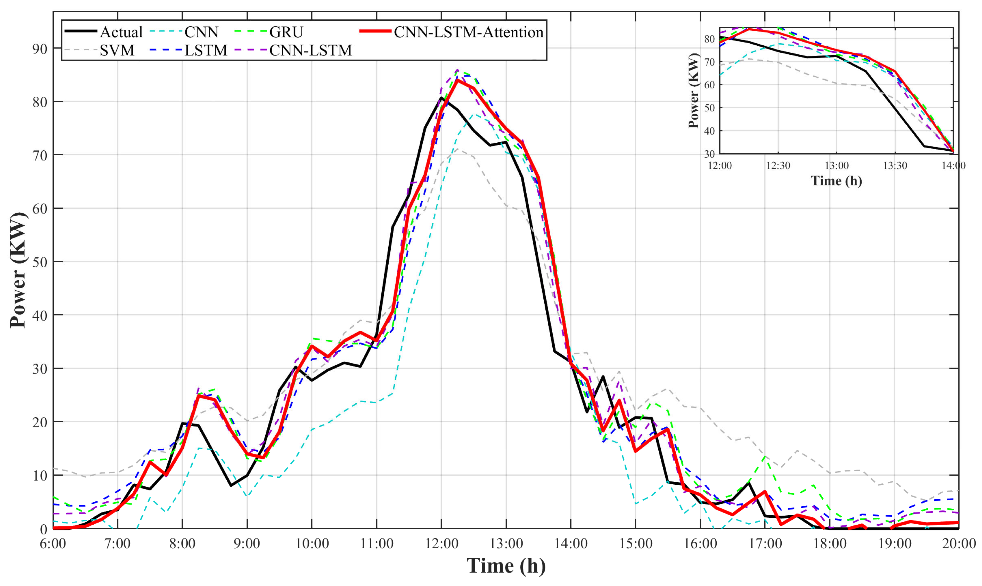
Winter days with high meteorological variability were selected to evaluate model resilience under extreme operating conditions. Table 5 and Figure 10 present quantitative metrics and temporal trajectories, detailing performance differences among photovoltaic forecasting architectures. Deep learning models generally outperform traditional methods; for instance, the support vector machine (SVM) yields an RMSE of 13.686 kW and a coefficient of determination of 0.770, struggling with high-frequency power shifts and producing phase-delayed, overly smoothed outputs [25]. Conversely, recurrent networks like LSTM and GRU achieve superior sequence decomposition (RMSE: 3.5–3.7 kW), overcoming the representational constraints of shallow models when processing complex, long-term meteorological dependencies. Hybrid architectures further improve predictive accuracy by integrating complementary spatiotemporal features. Independent CNNs (RMSE: 5.555 kW) underperform recurrent models, yet pure RNNs struggle to extract spatial coupling within multivariate data. Consequently, the CNN-LSTM hybrid reduces the RMSE from the 3.714 kW LSTM baseline to 2.582 kW (a 30.47% reduction). This indicates that combining front-end CNN local pattern extraction with back-end LSTM long-term trend modeling captures complex spatiotemporal dynamics more effectively than isolated models.
Table 5.
Performance comparison of different prediction models.
Figure 10.
Forecasting performance comparison over a typical winter day. The inset provides a magnified view of the 12:00–14:00 interval, highlighting the superior tracking accuracy of the proposed CNN–LSTM–Attention model during peak power fluctuations.
To benchmark the adopted model against recent architectures (Table 5, Figure 10), the Transformer yields an RMSE of 3.084 kW but overestimates noon peak power. While the TCN-Attention model improves accuracy (RMSE: 2.857 kW), its prediction curve displays local sawtooth fluctuations, struggling to track declining trends smoothly. We adopt the CNN–LSTM–Attention model, which maintains the lowest RMSE (2.157 kW) and accurately matches the actual power curve, demonstrating structural advantages in extracting short-term local features. Compared to the CNN-LSTM baseline, this design reduces the RMSE to 2.157 kW (a 16.46% decrease) and the MAE to 1.432 kW, while increasing the coefficient of determination to 0.991. Acting as a dynamic feature identification system, the attention mechanism accurately monitors peak power fluctuations. Ultimately, the framework predicts non-stationary sequences by combining CNN spatial extraction, LSTM temporal modeling, and the SE-based attention mechanism [26].
To measure temporal tracking, cross-correlation and Dynamic Time Warping (DTW) were employed for phase lag and morphological synchronization analyses, respectively. Raw 15 min sequences were up-sampled to 1 min intervals via cubic spline interpolation to permit continuous measurement. DTW evaluates morphological similarity by warping the time axis, detecting temporal misalignments and structural distortions. As detailed in Table 5, the CNN–LSTM–Attention model achieved the lowest absolute DTW distance (6908.77), indicating the attention mechanism corrects phase shifts and preserves morphological fidelity. In contrast, the LSTM baseline recorded a higher DTW (8994.54) with a 6 min phase lag. While the Transformer reduced this lag to 4 min, its elevated DTW (8705.42) suggests predicted sequences suffer from morphological inconsistencies despite capturing broad temporal dependencies. The TCN-Attention model (8600.50) also underperformed the CNN-LSTM baseline (8159.17), as localized shape fluctuations increased structural alignment penalties. To standardize temporal alignment comparisons regardless of sequence length, a normalized DTW metric was used. The CNN–LSTM–Attention model attained the lowest normalized DTW (0.874), confirming its accuracy in tracking rapid phase shifts and maintaining the power curve’s structural integrity compared to baseline architectures.
The Diebold–Mariano (DM) test was used to establish that our CNN–LSTM–Attention model achieved a statistically significant performance improvement (Root Mean Square Error: 2.157 kW) compared to the baseline CNN-LSTM model (Root Mean Square Error: 2.582 kW) through analysis of squared prediction errors. The null hypothesis posited equal prediction accuracy between the two models. Test results yielded a DM statistic of 12.765 and a value of 0.0008 (). Since the value falls well below the 5% significance threshold, the null hypothesis is rejected. The findings indicate that the suggested SE-based attention technique surpasses the static baseline, according to the statistical analysis.
Furthermore, the performance of our architecture aligns with, yet clearly improves upon, findings in the recent literature. For instance, while previous research established the effectiveness of CNN-LSTM networks, their static architectures struggled with sudden weather regime shifts, resulting in noticeable phase lags. Similarly, models employing general attention structures often experience peak-shaving during high-frequency fluctuations. The specific SE-based attention strategy implemented in this study resolves these limitations, achieving an RMSE of 2.157 kW. This confirms its specific utility and reliability for regions with highly volatile climates like that of Ningxia, distinguishing our framework from standard hybrid approaches.
4.2. Overall Prediction Performance Evaluation
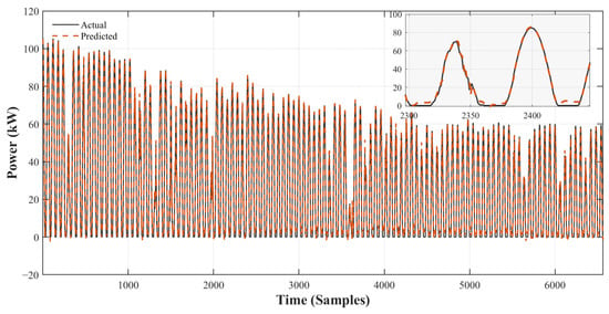
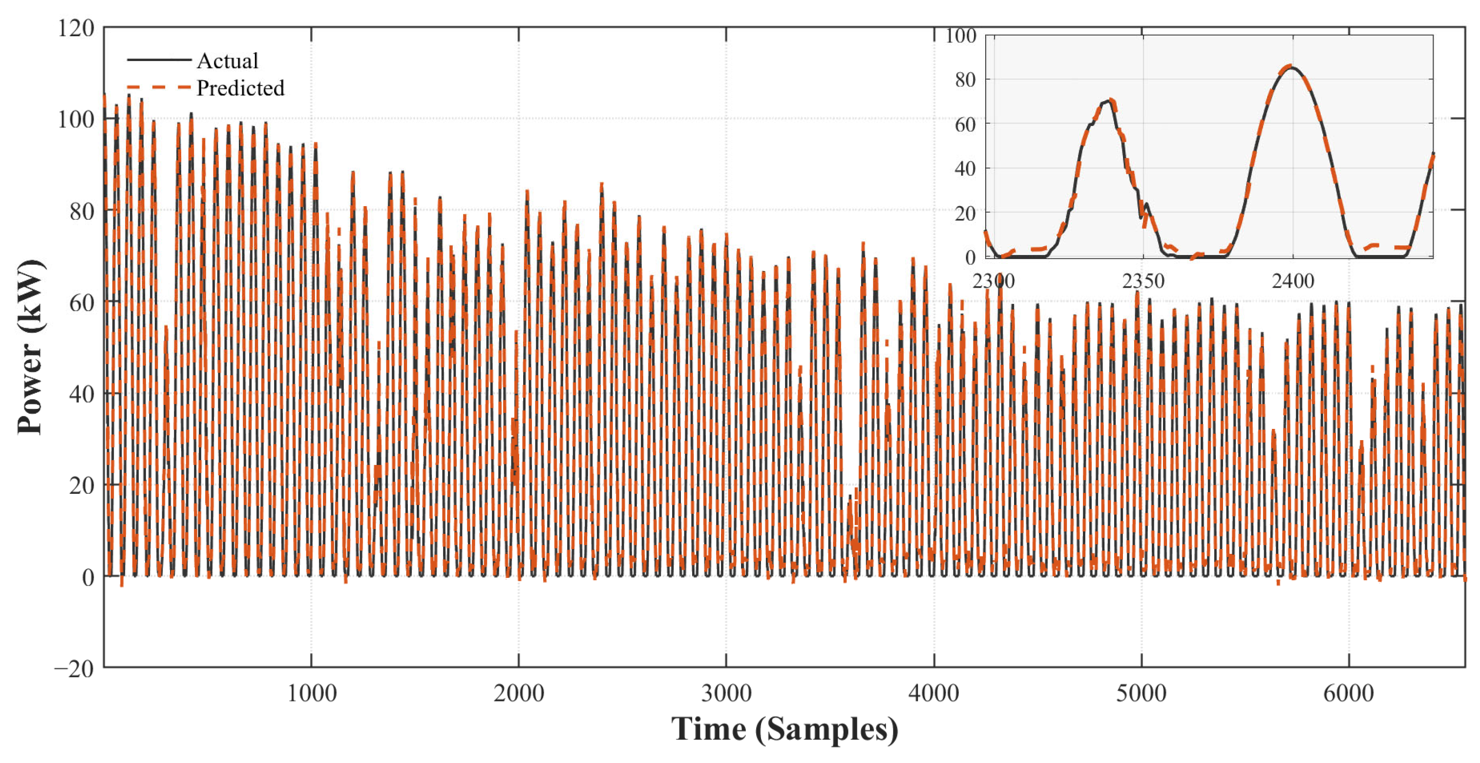
The generalization performance of the CNN–LSTM–Attention model for long time series and multiple seasonal periods is evident in Figure 11, which shows the model’s predicted values against actual test set values.
Figure 11.
Annual PV power prediction results. The graph illustrates the recorded power data and the estimates from the CNN–LSTM–Attention network across a full calendar year. The time series is organized to display the seasonal variations in solar output from January to December.
The black solid and orange dashed lines indicate the actual and predicted values, respectively, which maintain a high degree of overlap across the entire period when viewed from a macroscopic perspective (main plot in Figure 3). The test set contains different seasonal weather conditions and solar radiation patterns; however, the predicted curve tracks the actual power output with small total prediction errors and minimal major pattern changes. The model demonstrates its ability to detect both nonlinear patterns and periodic behavior that exist in the photovoltaic power sequence.
The model fits both the peak and trough regions in the microscopic data with minimal bias (Figure 3 magnified view). Throughout all times when photovoltaic production fluctuates, the projected curve precisely tracks the actual values without any delays. The consistency and stability demonstrated by this model on long-term data prove that it has excellent generalization ability [27]. This system can adapt to changes in meteorological conditions under different circumstances and times of the year.
4.3. Performance Analysis Under Different Weather Conditions
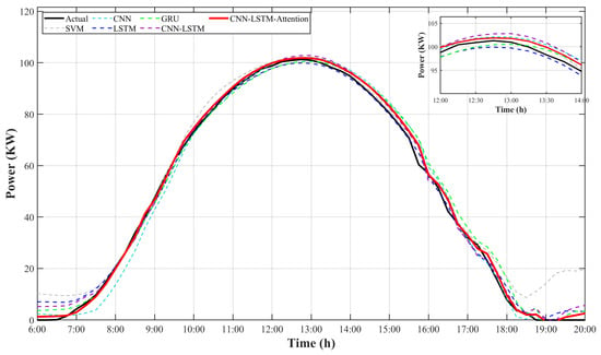
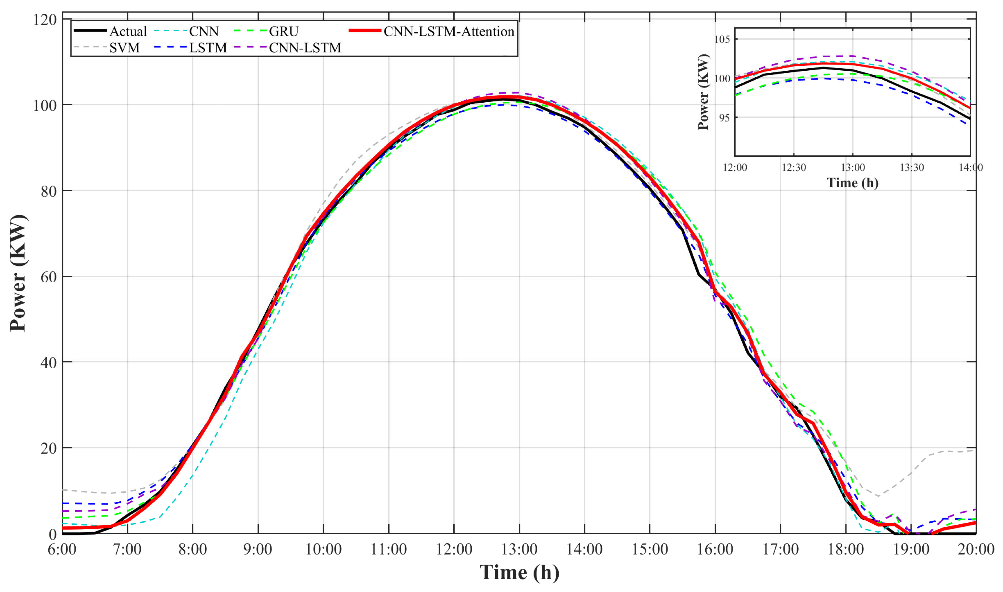
PV power production is significantly affected by weather conditions, revealing considerable intermittency and volatility. In this study, we selected three common weather conditions from the test dataset—sunny, cloudy, and rainy—to comprehensively evaluate performance. The CNN–LSTM–Attention model demonstrated robust performance under challenging meteorological conditions. The prediction outcomes are shown in Figure 10, Figure 11 and Figure 12. To prevent excessive curve overlap and ensure graphical readability, the Transformer and TCN-Attention were excluded from this typical day comparison.
Figure 12.
Sunny day comparison chart. The graph shows the power forecasting results of the CNN–LSTM–Attention network and comparison models under clear sky conditions. The inset window provides a closer view of the power output trends from 12:00 to 14:00.
First, as illustrated in Figure 12, under clear conditions, air transparency increases, and irradiance varies gradually. This phenomenon generates a power curve that consistently has a parabolic shape. This trend occurs while most deep learning models can discern the general trend of solar power output. Comparative models—such as LSTM and GRU—have amplitude discrepancies at the midday radiation peak time (12:00–13:00). Such discrepancies are inadequately aligned with the real peak. Conversely, the CNN–LSTM–Attention model effectively captures power peaks because of its attention mechanism’s adaptive [16] weighting for crucial time steps. These mechanisms provide superior prediction accuracy in stable situations.
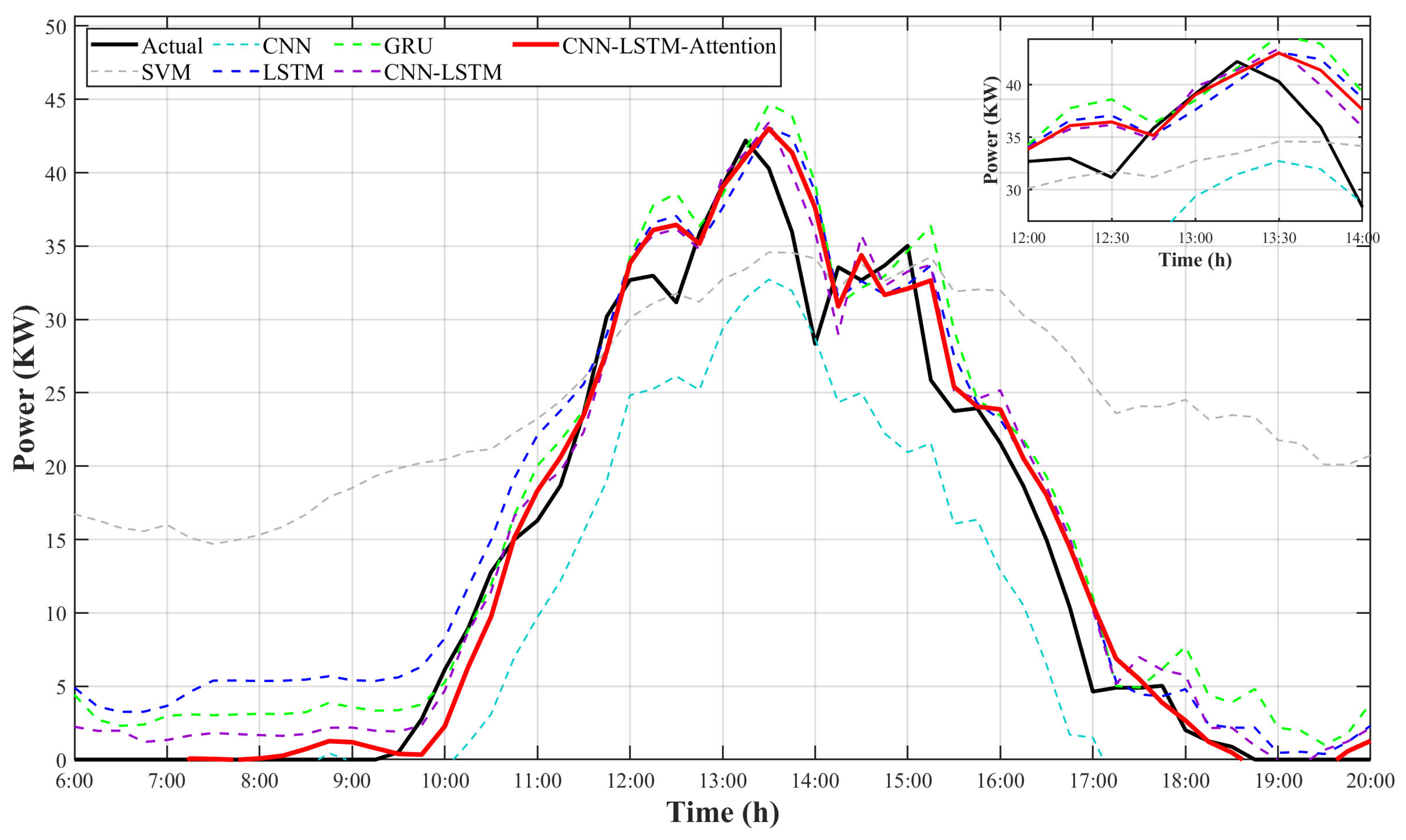
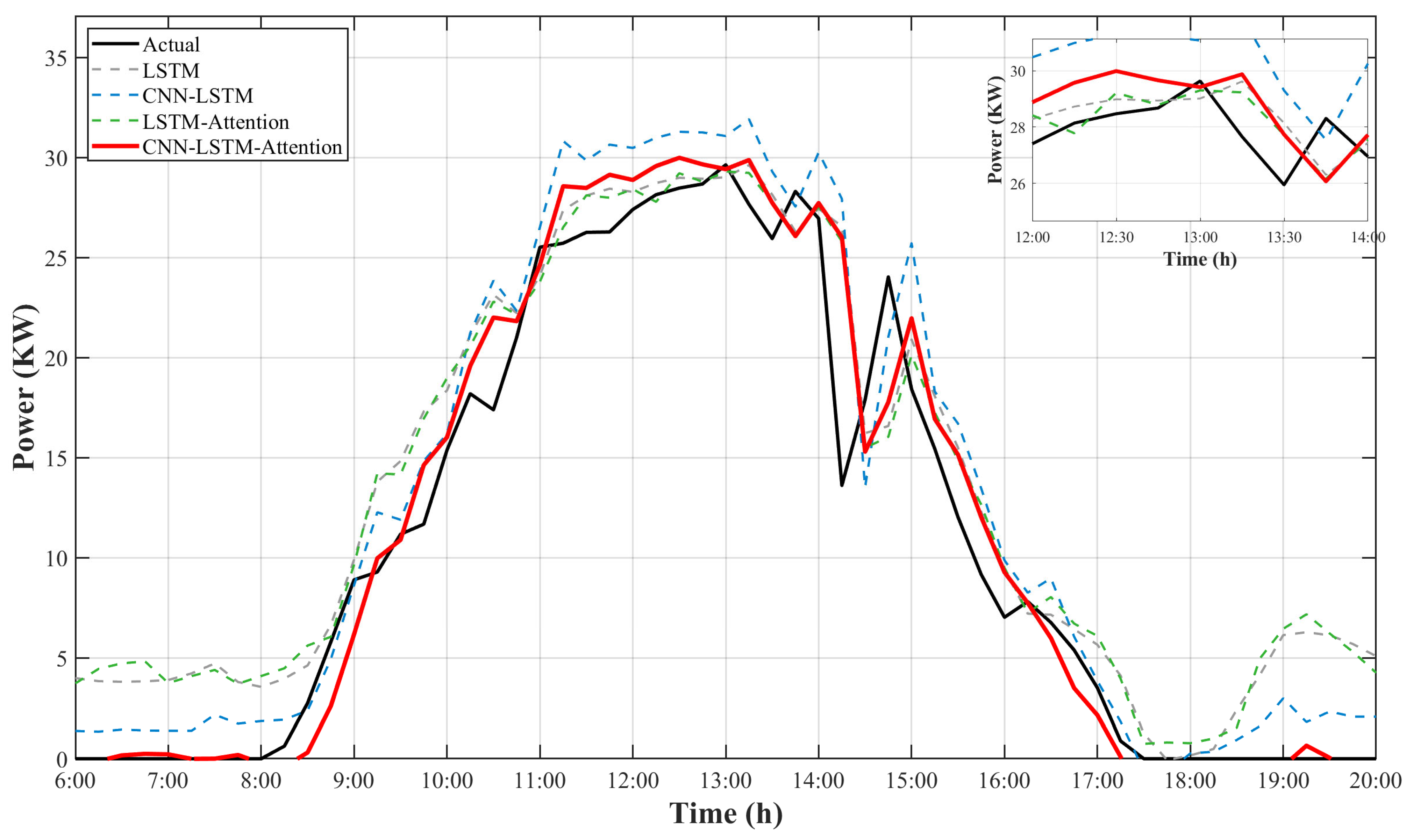
Second, Figure 13 shows the predictive outcomes under overcast conditions. The photovoltaic output experiences significant non-stationary shifts owing to cloud occlusion and rapid movement, resulting in a distinct “sawtooth” pattern in the curve. The expanded portion clearly illustrates that conventional shallow models, such as support vector machines (SVMs) and specific recurrent neural networks, display considerable latency in addressing abrupt power fluctuations [28]. These systems inadequately respond in real time to rapidly changing power data. The hybrid model we adopted efficiently recovers local fluctuation information via the convolutional layer of the convolutional neural network (CNN) and captures long-term dependencies via the long short-term memory network (LSTM). This structure thereby addresses the phase-lag problem. Importantly, this model consistently exhibits high synchronization with real values, even during times of strong oscillation.
Figure 13.
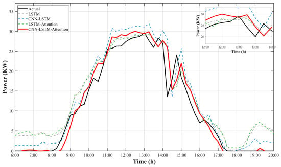
Cloud comparison chart. The plot illustrates the time-series forecasting of PV power output under cloudy sky conditions, involving the proposed CNN–LSTM–Attention network and several benchmark models. An inset is included to provide a magnified view of the power generation sequence from 12:00 to 14:00.
The rainstorm conditions in Figure 14, characterized by reduced irradiance and high noise, yield lower power amplitudes with random disturbances. Between 14:00 and 18:00, when actual power is low, the GRU and CNN-LSTM baselines produce overestimations and oscillatory errors, missing minor trend variations. Conversely, the proposed model filters input disturbances, maintaining stability and tracking precision in near-zero-power environments. This adaptability across diverse weather conditions, including sunny and overcast states, indicates its reliability for grid-connected photovoltaic applications compared to benchmarks. Practically, the forecasting improvements of the SE-based attention model offer three operational benefits: improving daily grid scheduling and resource dispatching, reducing the need for costly spinning reserves by minimizing prediction error margins, and increasing renewable energy integration to support sustainable power generation. Although the CNN–LSTM–Attention architecture requires higher computational resources during initial training, this process is executed offline. The online inference phase relies on a single forward propagation, satisfying the latency requirements of real-time grid applications.
Figure 14.
Solar power prediction results for a rainy day. The curves compare the CNN-LSTM-Attention model with other methods. The inset shows a zoomed-in view of the local prediction performance.
4.4. Ablation Studies
Ablation studies were conducted to assess the individual contributions and combined effects of the framework’s core components. The research team chose winter cloudy wave weather conditions for testing because they needed to verify how each module performs when dealing with quick changes in meteorological data. The performance metrics for different model variants are summarized in Table 6, with their time-series prediction trajectories and local magnified views shown in Figure 13.
Table 6.
Performance comparison of ablation experiments.
The default LSTM model demonstrates considerable performance deficiencies, with a Root Mean Square Error (RMSE) of 3.714 kW. As indicated by the gray dashed line, while the model tracks the overall trend of irradiance, it exhibits severe “inertial lag” and “over-smoothing.” Because it lacks a spatial feature extraction mechanism, a standalone LSTM cannot decipher complex nonlinear relationships among multiple input variables, thereby restricting its ability to detect rapid pattern changes.
The model attained improved outcomes with the incorporation of a convolutional neural network (CNN) module, resulting in the CNN–LSTM architecture, which obtained a Root Mean Square Error of 2.582 kW. The time-domain waveform analysis indicates that the convolutional kernels in the model effectively reduced background noise present during low irradiance periods by analyzing local morphological aspects. In the absence of an attention mechanism, the model exhibited greater sensitivity during the midday high-power period. This is seen by the blue dashed line in Figure 15, which shows ablation study results. This research demonstrates that traditional feature combination techniques are inadequate. They cannot modulate the significance of input data variables. Small shifts in secondary feature values, like wind speed variations [29], often trigger disproportionate model reactions.
Figure 15.
Performance analysis of various model architectures for PV power forecasting. The curves compare the integrated CNN-LSTM-Attention network with its individual sub-models under volatile conditions. The inset highlights the prediction accuracy during periods of high volatility.The model tracks the system with high accuracy, as indicated by the red solid line in Figure 15 during the 14:30 transient drop scenario, which shows a deep V-shaped decline in the signal. The SE-based attention of the model responds immediately to all fast-changing signals. This research confirms an important engineering principle, indicating that non-stationary PV power forecasting produces superior results by uniting spatial feature extraction with adaptive feature-weighting techniques. The two elements work together as essential components that solve the two main problems of baseline drift and phase lag. The model demonstrates its effectiveness through this occurrence because it detects the beginning of cloud cover and then readjusts its weight distribution to focus on cloud cover events instead of past power consumption patterns. Without this module, the network would experience an inevitable response delay owing to its inability to dynamically shift focus. The improved transient tracking ability proves that our SE-based attention operates according to physical principles [30].
The LSTM−Attention architecture, which used only the self-attention mechanism, achieved a Root Mean Square Error of 2.4576 kW while reducing overestimation during high power consumption. The model showed minimal “zero drift” during periods of low irradiance, which occurred during dawn and dusk (Figure 15 shows the green dashed line remaining above the zero axis). This observation suggests that the attention mechanism alone struggles to fully separate weak effective signals from sensor background noise in high-dimensional feature spaces [29]. This difficulty exists without the prerequisite of local morphological filtering based on convolutional neural networks. Nevertheless, the overall prediction accuracy of the LSTM−Attention model remained marginally higher than that of the convolutional neural network−long short-term memory (LSTM) model. A quantitative analysis indicates that dynamic feature weight adjustment is more critical than mere spatial extraction during rapid weather transitions. The CNN–LSTM–Attention hybrid architecture achieved optimal prediction performance by fully integrating spatial morphological filtering with SE-based attention, resulting in a Root Mean Square Error of 2.157 kW and value of 0.991. The model integrates extensive noise mitigation with precise error correction. The front-end CNN reduces sensor baseline noise during twilight, whereas the rear-end spatial attention mechanism discerns significant variation factors during peak power intervals, thereby diminishing excessive oscillations.
4.5. Goodness-of-Fit and Error Distribution Characteristics
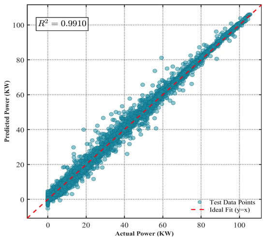
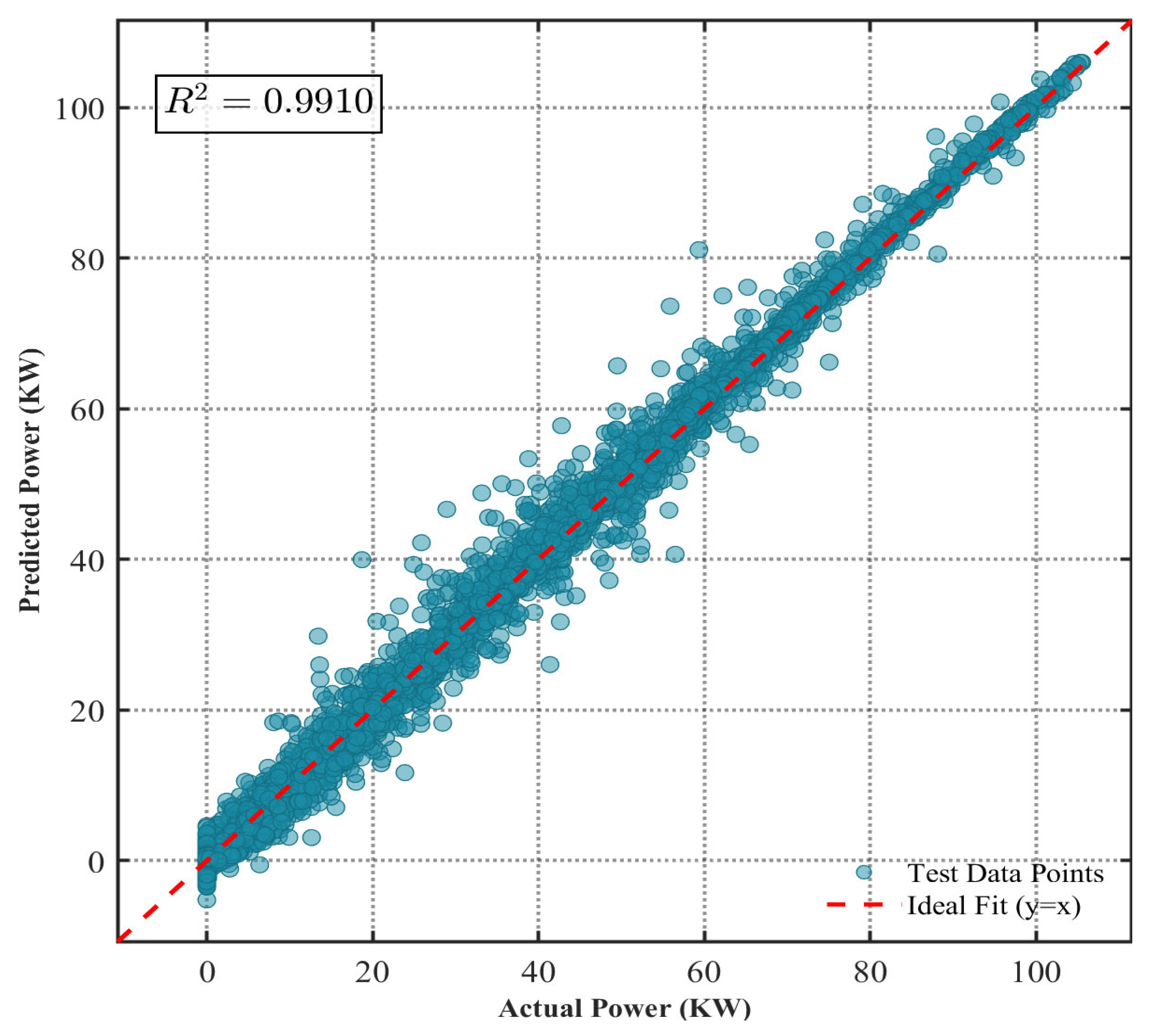
The analysis in this section proves the model’s ability to predict under various weather conditions using two methods that examine the distribution of predicted values and the time-dependent patterns of residual data. The CNN–LSTM–Attention architecture extracts spatiotemporal features which create a linear relationship with actual power output at a coefficient of determination value of 0.991, as shown in Figure 16. The system operates differently than typical deep learning models do when they achieve their peak performance in extreme value regions. The adopted model exhibits convergence properties along the diagonal. The system operated without phase lag or peak clipping when it tracked actual values at high irradiance levels which exceeded 80 kW.
Figure 16.
Scatter plot of predicted versus actual PV power. Each point represents a test data sample, displaying the relationship between the recorded power and the model estimates. The red dashed line indicates the ideal reference, with the coefficient of determination () labeled in the top-left corner.
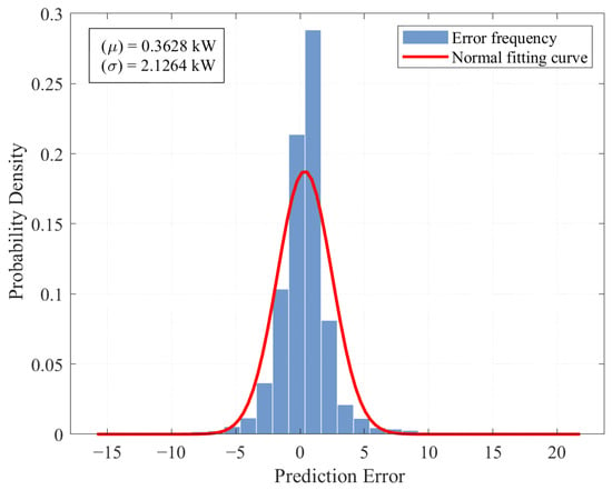
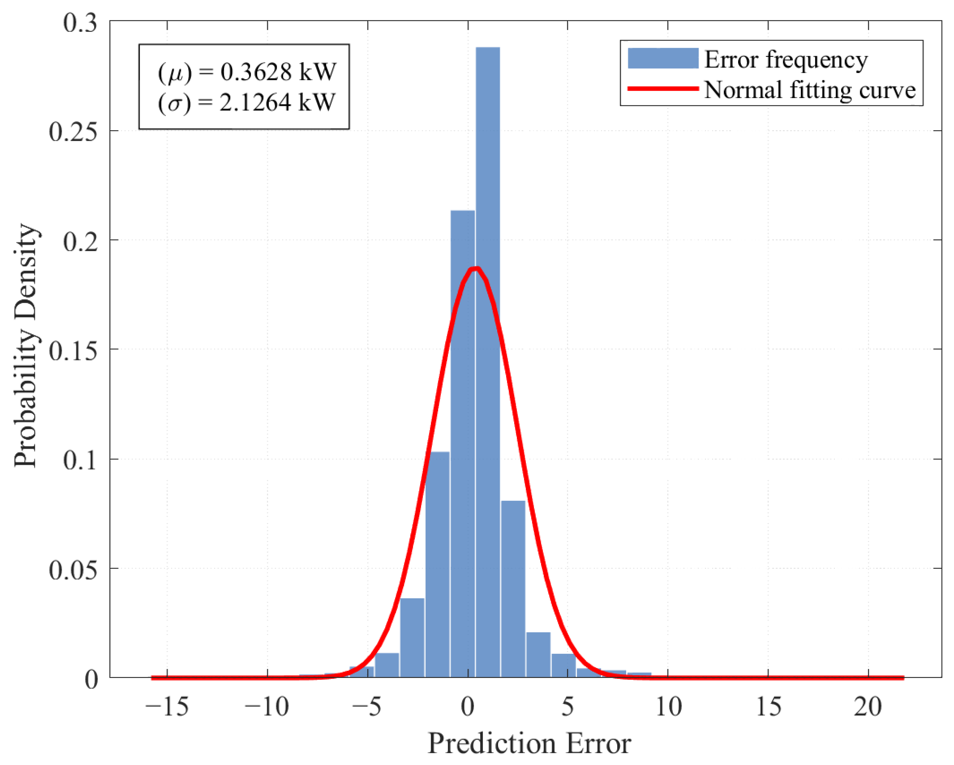
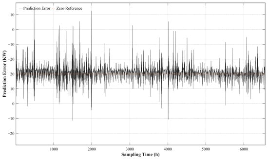
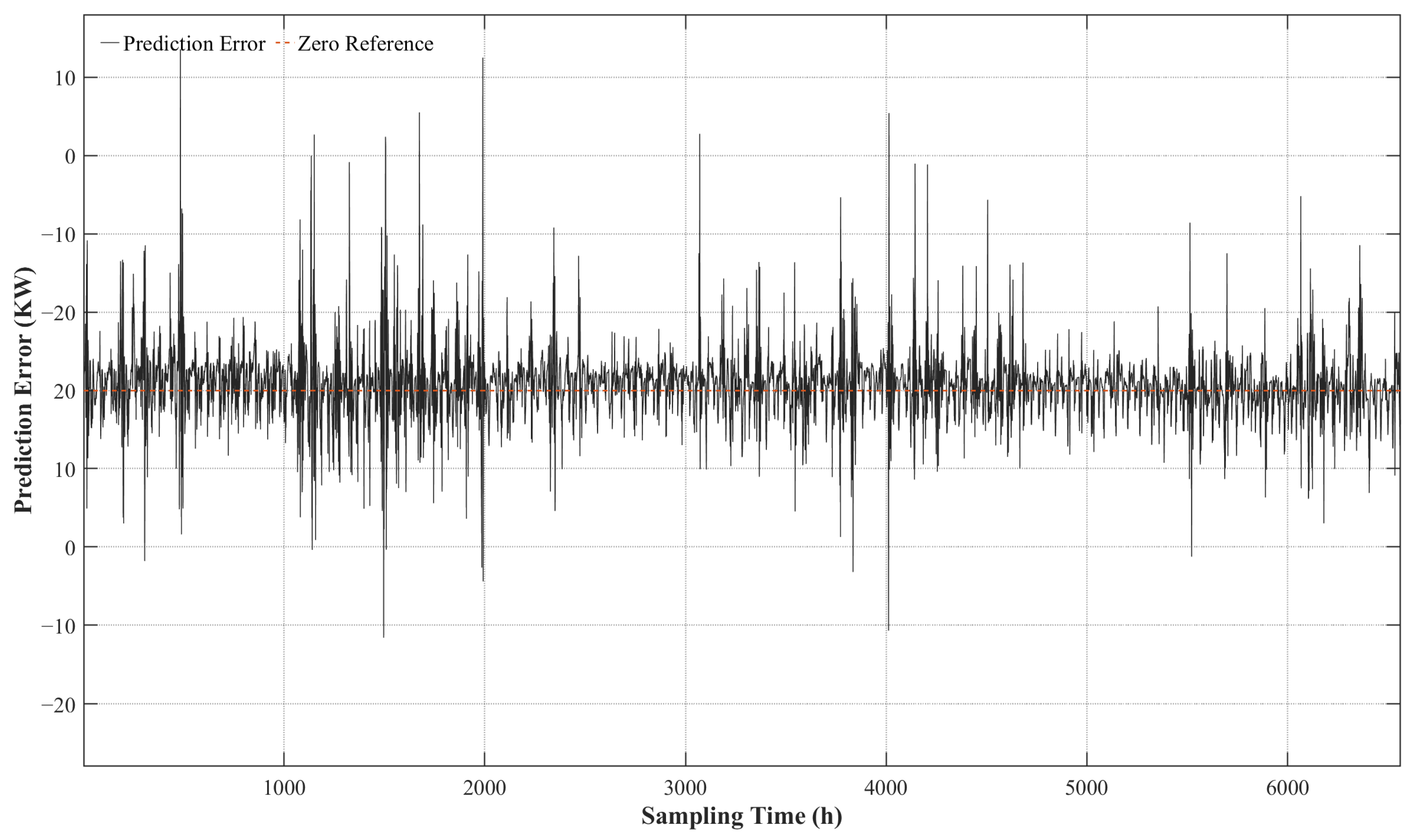
The error probability distribution illustrates the model’s efficacy in providing unbiased estimations with its capacity to accurately fit the data. Figure 17 illustrates that prediction errors display a peaked distribution, in contrast to the broad-tailed features of a regular normal distribution. The probability density is confined to a zero-centered bandwidth of kW. The zero-symmetric distribution pattern indicates an absence of systematic bias, demonstrating that cloud movement does not induce significant errors [31]. The model effectively reduced systematic bias, as evidenced by the observed leptokurtic distribution, which indicates that significant errors arise solely during atypical and physically implausible abrupt cloud motions. The error distribution pattern offers several benefits to grid operators, as it indicates that the majority of faults occur at zero value, thereby reducing operational uncertainty and minimizing the requirement for spinning reserve capacity during base-load operations. The residual sequence analysis in the time domain (Figure 18) indicates that the signal exhibits zero mean stationarity and white noise characteristics. To statistically characterize this, basic metrics were calculated: the mean error () is 0.3628 kW, suggesting a low level of systematic bias, and the standard deviation () is 2.1264 kW, which explicitly quantifies the magnitude of the random noise. This statistical evidence suggests that the approach effectively recovered the main deterministic spatiotemporal patterns from the input data. The residual sequence had remarkable recovery abilities, reverting to its original form following adverse weather conditions at point 500. The LSTM gating mechanism, in conjunction with the attention technique, effectively mitigated the propagation of past mistakes across time [32].
Figure 17.
Probability distribution of prediction errors. The histogram illustrates the frequency of residuals between the predicted and actual PV power. The red solid line represents the normal distribution fitting curve applied to the error data. The mean and standard deviation of the distribution are indicated in the top-left annotation box.
Figure 18.
Time-domain error residual sequence. The plot presents the residuals between the predicted and actual PV power values across the sampling interval. The horizontal dashed line serves as the zero-error reference.
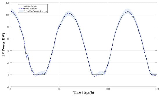
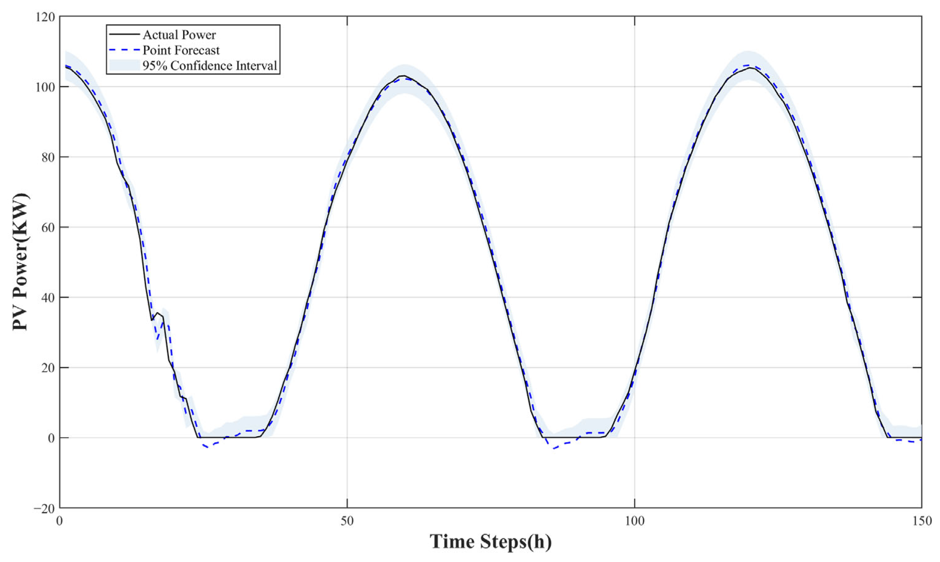
To support grid risk management, we extended our deterministic results into a probabilistic evaluation. The error distribution histogram and residual scatter (Figure 15) demonstrate a concentrated error distribution with a standard deviation of . Using this statistical baseline, we established a 95% probabilistic prediction interval (). The resulting shaded uncertainty band (Figure 19) directly supplies grid operators with quantified safety margins for reliable reserve planning.
Figure 19.
Point forecast with confidence intervals. The plot displays the predicted PV power values against the actual measurements over 150 time steps. The shaded region denotes the 95% confidence interval, quantifying the uncertainty associated with the point estimates across the sampling period.
5. Conclusions
5.1. Research Findings
To address accuracy limitations and phase lag in photovoltaic power forecasting under complex meteorological conditions, in this paper, we adopt a hybrid framework integrating convolutional neural networks (CNNs), long short-term memory (LSTM) networks, and attention mechanisms. Validation using real-world data from a 150 kW photovoltaic power station in Ningxia yields the following key outcomes:
Effective Spatiotemporal Integration: The integration of a CNN for front-end spatial filtering and an LSTM for temporal modeling effectively resolves the peak clipping issue common in standalone recurrent networks.
Phase Lag Reduction: The SE-based attention mechanism acts as an adaptive weight controller to dynamically adjust feature responses. Dynamic Time Warping (DTW) evaluations confirm that this specific design successfully corrects temporal delays and phase shifts.
Significant Accuracy Improvements Across Varied Conditions: Benchmark comparisons confirm the effectiveness of the adopted model across different weather states, particularly during volatile cloudy and rainy conditions. The framework achieved a Root Mean Square Error (RMSE) of 2.157 kW and an value of 0.991. This performance sharply outperforms conventional shallow methods and recent deep learning architectures like the Transformer and TCN-Attention. Specifically, the model reduced the RMSE by 84.2% and 42.0% compared to the SVM and standalone LSTM models, respectively. Furthermore, ablation analysis proves that combining spatial morphological filtering with the SE-based attention mechanism is strictly necessary. This specific design minimizes residuals during rapid weather transitions and manages non-stationary sequences with high reliability.
Statistical Reliability: The Diebold–Mariano test quantitatively confirmed that the performance improvement over baseline models is statistically significant. Additionally, residual sequence analysis revealed a zero-centered leptokurtic distribution with white noise characteristics, indicating minimal systematic bias. This provides reliable point forecasting support for grid dispatch decisions.
5.2. Limitations and Future Work
While demonstrating reliable tracking accuracy, the CNN–LSTM–Attention framework possesses experimental constraints requiring further investigation. Utilizing data primarily from the Ningxia region—characterized by a temperate continental climate, frequent sandstorms, high irradiance, and low humidity—the study’s geographic scope is limited. Consequently, the performance of the adopted model across diverse meteorological conditions, including humid tropical, coastal, or high-altitude environments, remains unverified. Nevertheless, the SE-based attention framework’s core methodology is geographically independent, allowing adaptation to new climates through retraining with local datasets. Future research will address this single-station limitation by incorporating data from varied photovoltaic plants to assess environmental adaptability. Furthermore, while the utilized 2019 dataset may exclude recent climate shifts or long-term panel degradation, short-term photovoltaic forecasting relies on immediate meteorological variables and high-frequency time-series patterns rather than macro-level trends. Thus, this temporal dataset remains suitable for verifying the adopted model’s short-term tracking capabilities. Second, the current validation relies on observed inputs to establish theoretical performance upper bounds; practical engineering applications require numerical weather prediction (NWP) data. Future research will develop error correction mechanisms to compensate for accuracy degradation caused by NWP forecast biases through postprocessing algorithms [33].
Additionally, to overcome the limitation of single-site prediction ignoring the correlation of surrounding cloud movement, future plans include introducing Graph Neural Networks (GNNs) to explicitly model spatiotemporal topological relationships within distributed PV clusters [11]. This approach aims to enhance ultra-short-term warning capabilities for minute-level power fluctuations by utilizing upstream power plant fluctuations as precursor signals. Finally, with the evolution of deep learning technologies, Transformer-based architectures demonstrate potential for handling ultra-long sequences. Frameworks like the Photovoltaic Multimodal Transformer (PVMTF) can effectively process photovoltaic data with complex dependencies through end-to-end long-sequence time-series prediction and information enhancement strategies [34]. Finally, the 150 kW system size evaluated in this study is relatively small. The scalability of the adopted framework to utility-scale photovoltaic plants in the MW range—which involve different panel technologies, inverter configurations, and wider spatial distributions—remains unverified at this stage. However, the data-driven architecture is highly modular. For large-scale applications, the forecasting system can be deployed in blocks based on specific individual inverters or subarrays. Because the mathematical mapping effectively relies on local meteorological inputs rather than absolute capacity values, the framework is scalable and not restricted by the total plant size.
Author Contributions
Conceptualization, M.L. and B.W.; methodology, M.L., T.C. and B.W.; software, M.L. and T.C.; validation, M.L., T.C. and C.Y.; formal analysis, M.L., T.C. and Y.X.; investigation, M.L., Y.X. and C.Y.; resources, M.L., C.Y. and Y.X.; data curation, M.L., T.C., Y.X. and C.Y.; writing—original draft preparation, M.L. and T.C.; writing—review and editing, M.L., S.W. and W.S.-N.; visualization and supervision, W.S.-N., S.W. and B.W.; project administration, W.S.-N. and B.W. All authors have read and agreed to the published version of the manuscript.
Funding
This research was funded by Mahasarakham University.
Data Availability Statement
The original contributions presented in the study are included in the article; further inquiries can be directed to the corresponding author.
Acknowledgments
This research project was financially supported by Mahasarakham University. The authors would like to express gratitude to the Electrical and Computer Engineering Research Unit, Faculty of Engineering, Mahasarakham University, and the College of Electrical Engineering, Hunan Mechanical & Electrical Polytechnic, for the facility support.
Conflicts of Interest
The authors declare no conflicts of interest.
References
- Asano, H.; Ishii, H.; Takano, H. Distributed Energy Resource Integration for Carbon Neutral Power Systems: Market-Based Approaches to Ancillary Services and Microgrid Operation. IEEJ Trans. Electr. Electron. Eng. 2024, 19, 598–607. [Google Scholar] [CrossRef] [Scilit]
- Tejero-Gómez, J.A.; Bayod-Rújula, Á.A. Analysis of Grid-Scale Photovoltaic Plants Incorporating Battery Storage with Daily Constant Setpoints. Energies 2024, 17, 6117. [Google Scholar] [CrossRef] [Scilit]
- Nakamoto, Y.; Eguchi, S. How Do Seasonal and Technical Factors Affect Generation Efficiency of Photovoltaic Power Plants? Renew. Sustain. Energy Rev. 2024, 199, 114441. [Google Scholar] [CrossRef] [Scilit]
- Lodhi, E.; Wang, F.-Y.; Xiong, G.; Mallah, G.A.; Javed, M.Y.; Tamir, T.S.; Gao, D.W. A Dragonfly Optimization Algorithm for Extracting Maximum Power of Grid-Interfaced PV Systems. Sustainability 2021, 13, 10778. [Google Scholar] [CrossRef] [Scilit]
- Deeum, S.; Bhumkittipich, P.; Janjamraj, N.; Romphochai, S.; Kongjeen, Y.; Bhumkittipich, K. Robust Optimization for PV and BESS Configurations in Distribution Network with EV Load Uncertainties. Eng. Access 2025, 11, 262–270. [Google Scholar]
- Xie, H.; Li, P.; Shi, F.; Han, C.; Cui, X.; Zhao, Y. Spatial and Temporal Expansion of Photovoltaic Sites and Thermal Environmental Effects in Ningxia Based on Remote Sensing and Deep Learning. Remote Sens. 2025, 17, 2440. [Google Scholar] [CrossRef] [Scilit]
- Zhang, X.; Zeraatpisheh, M.; Rahman, M.M.; Wang, S.; Xu, M. Texture Is Important in Improving the Accuracy of Mapping Photovoltaic Power Plants: A Case Study of Ningxia Autonomous Region, China. Remote Sens. 2021, 13, 3909. [Google Scholar] [CrossRef] [Scilit]
- Mellit, A.; Pavan, A.M.; Ogliari, E.; Leva, S.; Lughi, V. Advanced Methods for Photovoltaic Output Power Forecasting: A Review. Appl. Sci. 2020, 10, 487. [Google Scholar] [CrossRef] [Scilit]
- Chooseang, T.; Prabpal, P.; Sonasang, S.; Angkawisittpan, N.; Nangtin, P. Optimal PV Sizing and Location Based on Volt-Var Control and UPFC Using Particle Swarm Optimization for Microgrid System. Eng. Access 2025, 12, 10–19. [Google Scholar]
- Qin, B.; Wang, M.; Zhang, G.; Zhang, Z. Impact of Renewable Energy Penetration Rate on Power System Frequency Stability. Energy Rep. 2022, 8, 997–1003. [Google Scholar] [CrossRef] [Scilit]
- Simeunovic, J.; Schubnel, B.; Alet, P.-J.; Carrillo, R.E. Spatio-Temporal Graph Neural Networks for Multi-Site PV Power Forecasting. IEEE Trans. Sustain. Energy 2022, 13, 1210–1220. [Google Scholar] [CrossRef] [Scilit]
- Spampinato, C.; Valastro, S.; Calogero, G.; Smecca, E.; Mannino, G.; Arena, V.; Balestrini, R.; Sillo, F.; Ciná, L.; La Magna, A.; et al. Improved Radicchio Seedling Growth under CsPbI3 Perovskite Rooftop in a Laboratory-Scale Greenhouse for Agrivoltaics Application. Nat. Commun. 2025, 16, 2190. [Google Scholar] [CrossRef] [Scilit] [PubMed]
- Zhang, E.; Hou, L.; Shen, C.; Shi, Y.; Zhang, Y. Sound Quality Prediction of Vehicle Interior Noise and Mathematical Modeling Using a Back Propagation Neural Network (BPNN) Based on Particle Swarm Optimization (PSO). Meas. Sci. Technol. 2016, 27, 015801. [Google Scholar] [CrossRef] [Scilit]
- Chen, S.; Lin, R.; Zeng, W. Short-Term Load Forecasting Method Based on ARIMA and LSTM. In Proceedings of the 2022 IEEE 22nd International Conference on Communication Technology (ICCT), Nanjing, China, 11–14 November 2022; pp. 1913–1917. [Google Scholar]
- Zhang, L.; Zhu, J.; Zhang, D.; Liu, Y. An Incremental Photovoltaic Power Prediction Method Considering Concept Drift and Privacy Protection. Appl. Energy 2023, 351, 121919. [Google Scholar] [CrossRef] [Scilit]
- Agga, A.; Abbou, A.; Labbadi, M.; Houm, Y.E.; Ou Ali, I.H. CNN-LSTM: An Efficient Hybrid Deep Learning Architecture for Predicting Short-Term Photovoltaic Power Production. Electr. Power Syst. Res. 2022, 208, 107908. [Google Scholar] [CrossRef] [Scilit]
- Li, G.; Ding, C.; Zhang, R.; Chen, Y.; Zhao, N.; Zhu, R. Short-Term Prediction of PV Power Based on Hybrid CNN-BiLSTM-Attention Model and VMD. In Proceedings of the 2023 6th International Conference on Energy, Electrical and Power Engineering (CEEPE), Guangzhou, China, 12–14 May 2023; pp. 998–1003. [Google Scholar]
- Shen, J.; Wu, W.; Xu, Q. Accurate Prediction of Temperature Indicators in Eastern China Using a Multi-Scale CNN-LSTM-Attention Model. arXiv 2024, arXiv:2412.07997. [Google Scholar] [CrossRef] [Scilit]
- Slater, L.J.; Arnal, L.; Boucher, M.-A.; Chang, A.Y.-Y.; Moulds, S.; Murphy, C.; Nearing, G.; Shalev, G.; Shen, C.; Speight, L.; et al. Hybrid Forecasting: Blending Climate Predictions with AI Models. Hydrol. Earth Syst. Sci. 2023, 27, 1865–1889. [Google Scholar] [CrossRef] [Scilit]
- Amirteimoury, F.; Memarzadeh, G.; Noori, H.; Keynia, F.; Heydari, A.; Fekih, A. A Novel Multi-Scale Feature Attention Network-Based Prediction Model for the Accurate Forecasting of Photovoltaic Power Generation. IEEE Access 2025, 13, 165173–165188. [Google Scholar] [CrossRef] [Scilit]
- Zhou, N.; Shang, B.; Xu, M.; Peng, L.; Feng, G. Enhancing Photovoltaic Power Prediction Using a CNN-LSTM-Attention Hybrid Model with Bayesian Hyperparameter Optimization. Glob. Energy Interconnect. 2024, 7, 667–681. [Google Scholar] [CrossRef] [Scilit]
- Visser, L.; AlSkaif, T.; Van Sark, W. Operational Day-Ahead Solar Power Forecasting for Aggregated PV Systems with a Varying Spatial Distribution. Renew. Energy 2022, 183, 267–282. [Google Scholar] [CrossRef] [Scilit]
- Zhou, Z.; Dai, Y.; Leng, M. A Photovoltaic Power Forecasting Framework Based on Attention Mechanism and Parallel Prediction Architecture. Appl. Energy 2025, 391, 125869. [Google Scholar] [CrossRef] [Scilit]
- Wang, F.; Li, J.; Zhen, Z.; Wang, C.; Ren, H.; Ma, H.; Zhang, W.; Huang, L. Cloud Feature Extraction and Fluctuation Pattern Recognition Based Ultrashort-Term Regional PV Power Forecasting. IEEE Trans. Ind. Appl. 2022, 58, 6752–6767. [Google Scholar] [CrossRef] [Scilit]
- Yang, Z.; Hu, W.; Yang, F.; Liu, R. Frequency Stability Analysis of Power System with Photovoltaic Frequency Regulation Considering Communication Delay. Front. Energy Res. 2023, 10, 1041841. [Google Scholar] [CrossRef] [Scilit]
- Li, Z.; Xu, R.; Luo, X.; Cao, X.; Du, S.; Sun, H. Short-Term Photovoltaic Power Prediction Based on Modal Reconstruction and Hybrid Deep Learning Model. Energy Rep. 2022, 8, 9919–9932. [Google Scholar] [CrossRef] [Scilit]
- Wan, A.; Chang, Q.; Khalil, A.-B.; He, J. Short-Term Power Load Forecasting for Combined Heat and Power Using CNN-LSTM Enhanced by Attention Mechanism. Energy 2023, 282, 128274. [Google Scholar] [CrossRef] [Scilit]
- Miraftabzadeh, S.M.; Longo, M. High-Resolution PV Power Prediction Model Based on the Deep Learning and Attention Mechanism. Sustain. Energy Grids Netw. 2023, 34, 101025. [Google Scholar] [CrossRef] [Scilit]
- Zhang, M.; Gao, Q.; Liu, B.; Zhang, C.; Zhou, G. A Method Based on CNN–BiLSTM–Attention for Wind Farm Line Fault Distance Prediction. Energies 2025, 18, 3703. [Google Scholar] [CrossRef] [Scilit]
- Bai, M.; Wang, R.; Lin, C.; Chen, Y.; Dong, F.; Zhou, Z.; Yang, X.; Liu, J.; Yu, D. Deep Multivariable Spatial Attention CNN-Based Spatial Grid NWP Error Correction for Accurate One-Day-Ahead Photovoltaic Power Forecast. Earth Sci. Inform. 2025, 18, 427. [Google Scholar] [CrossRef] [Scilit]
- Ghimire, S.; Deo, R.C.; Raj, N.; Mi, J. Deep Solar Radiation Forecasting with Convolutional Neural Network and Long Short-Term Memory Network Algorithms. Appl. Energy 2019, 253, 113541. [Google Scholar] [CrossRef] [Scilit]
- Liu, W.; Mao, Z. Short-Term Photovoltaic Power Forecasting with Feature Extraction and Attention Mechanisms. Renew. Energy 2024, 226, 120437. [Google Scholar] [CrossRef] [Scilit]
- Thipwangmek, N.; Suetrong, N.; Taparugssanagorn, A.; Tangparitkul, S.; Promsuk, N. Enhancing Short-Term Solar Photovoltaic Power Forecasting Using a Hybrid Deep Learning Approach. IEEE Access 2024, 12, 108928–108941. [Google Scholar] [CrossRef] [Scilit]
- Tian, Z.; Liang, B. PVMTF: End-to-End Long-Sequence Time-Series Forecasting Frameworks Based on Patch Technique and Information Fusion Coding for Mid-Term Photovoltaic Power Forecasting. Appl. Energy 2025, 396, 126263. [Google Scholar] [CrossRef] [Scilit]

Disclaimer/Publisher’s Note: The statements, opinions and data contained in all publications are solely those of the individual author(s) and contributor(s) and not of MDPI and/or the editor(s). MDPI and/or the editor(s) disclaim responsibility for any injury to people or property resulting from any ideas, methods, instructions or products referred to in the content. |
© 2026 by the authors. Licensee MDPI, Basel, Switzerland. This article is an open access article distributed under the terms and conditions of the Creative Commons Attribution (CC BY) license.