Definition of Features for GIS Partial Discharge Signals and Recognition of Discharge Types Based on Histograms

Abstract

Different types of partial discharge (PD) cause varying degrees of insulation damage in gas-insulated switchgear (GIS), making accurate recognition of discharge types crucial for the safe and stable operation of GIS. The PD signal analysis method, including feature definition and extraction, is the foundation for recognizing discharge types. This paper first presents some measurement results of four PD types obtained on a GIS experimental platform. By analyzing the measurement results and corresponding physical mechanisms, we proposed two histogram-based features, which are discharge count versus phase histogram and discharge count versus amplitude histogram. To leverage the complementary advantages of these two features, distance-level fusion is achieved based on histogram distance. Following feature fusion, a distance-based k-nearest neighbors (KNN) classifier is used to recognize the four PD types. Compared with traditional feature fusion methods using feature concatenation, distance-level fusion improves recognition accuracy. The proposed PD type recognition method is also compared with two existing methods: one based on statistical features and another based on phase-resolved partial discharge (PRPD) image features. The results show that the proposed method achieves better recognition performance, with an accuracy of 95.8%.

1. Introduction

Gas-insulated switchgear (GIS) is widely used in power systems due to its compact structure and high reliability. The detection and identification of partial discharge (PD) in GIS is of great significance for its safe and reliable operation. Whether the electrical equipment has PD can be determined by electrical, acoustic, optical, or chemical detection [1,2,3]. Different types of PD can cause varying degrees of insulation damage. In equipment operation and maintenance, maintenance approaches are generally adopted based on PD type. Therefore, accurate recognition of PD types is vital for operational decision-making. The recognition relies on the analysis of PD signals. The key is to define and extract signal features that can distinguish different types of PD [4,5,6].

Partial discharge signals are primarily described in terms of time-domain waveforms and phase-resolved partial discharge (PRPD) spectra or phase-resolved pulse sequence (PRPS) spectra. Time-domain features such as rise time, fall time, and pulse width can be extracted from time-domain waveforms [7,8]. Alternatively, methods such as the short-time Fourier transform [9], wavelet transform [10], and S-transform [11] can convert time-domain waveforms into the frequency domain to extract frequency-domain or time-frequency features. While time-domain feature extraction is straightforward, it often yields poor recognition results for PD types. Time-frequency features can achieve good recognition performance but require complex signal processing techniques.

The PRPD spectrum plots the discharge count n, discharge amplitude q, and discharge phase $\phi$ on a two-dimensional plane. PRPD spectra of different PD types typically exhibit distinct characteristics [12]. Features based on the PRPD spectrum primarily fall into two categories: statistical features and image features.

Statistical feature extraction treats the PRPD spectrum as a distribution over n, q, and $\phi$. First, distributions such as n~q, n~$\phi$, and $q_{avg}\sim \phi$ are derived from the PRPD. Then, the mean, variance, skewness, kurtosis, etc., of these distributions are used as statistical features [13,14]. Reference [14] used the PD pulse count ratios in every 30-degree phase interval, along with the kurtosis and skewness of both positive and negative polarity half-cycles, as PRPD features. These were input alongside time-domain and frequency-domain features into a random forest (RF) for PD type recognition, achieving an accuracy of 93%. Statistical features are easy to extract and have clear physical interpretations. However, these statistics struggle to capture local details within the PRPD spectrum, thereby affecting the accuracy of subsequent PD type recognition.

Image features are texture or shape features, such as the gray-level co-occurrence matrix (GLCM) [15], local binary pattern (LBP) [16], and histogram of oriented gradients (HOG) [17], extracted from PRPD grayscale images. Reference [17] extracted HOG features from PRPD grayscale images and achieved 99% classification accuracy using the gradient boosting decision tree (GBDT) as the classifier. Image features primarily rely on texture or on properties such as translation and rotation invariance found in real photographs. However, PRPD spectra are graphs generated from PD data, lacking the texture of real photographs and exhibiting invariance only in certain directions. Consequently, while image features can achieve good recognition results, they are not specifically designed for PRPD spectra and typically involve high feature dimensions and computational complexity.

After obtaining PD signal features, a classifier is typically used for PD type recognition. Commonly used classifiers include k-nearest neighbors (KNN), support vector machine (SVM), RF, GBDT, and artificial neural network (ANN) [18,19,20,21,22]. In recent years, with the tremendous success of deep learning (DL) in the fields of vision and natural language processing, it has also been applied to PD type recognition. DL-based PD type recognition eliminates the need for manually designed features. Instead, it trains deep neural networks to automatically extract features from time-domain waveforms or PRPD spectra for classification [23,24,25]. However, compared to traditional classifiers, DL requires substantial training data and computational resources and suffers from poor interpretability.

Defining and extracting PD signal features primarily faces the trade-off between representational capability and computational complexity. To address this issue, this paper proposes two histogram-based features for PD signals, including discharge count versus phase histogram (DCPH) and discharge count versus amplitude histogram (DCAH). These two features use histograms to describe the phase distribution and amplitude distribution of PD signals, respectively. Feature extraction and analysis are straightforward, with low computational complexity, and they can capture local details of the phase and amplitude distributions. To comprehensively leverage the advantages of both features, a distance-level feature fusion method based on histogram distance is proposed. After obtaining the fused distance, the distance-based classifier KNN is used to recognize PD types. Finally, comparative and feature-ablation experiments validate the effectiveness of the proposed features and recognition method.

This paper is organized as follows: Section 2 presents the experiments on four types of PD in GIS; Section 3 defines PD signal features based on histograms and provides typical features for the four PD types; Section 4 describes a PD type recognition method based on histogram distance and its performance; Section 5 concludes the paper.

2. Experiments on Four Types of PD in GIS

To obtain signals of four PD types, including conductor protrusion discharge (Type P), floating conductor discharge (Type F), internal void discharge (Type V), and surface discharge (Type S), we conducted PD experiments on the experimental GIS platform. Different types of discharge electrodes were installed within the GIS chamber to generate different PD signals. The PD signals were measured using the pulse current method for discharge current signals and the ultra-high-frequency (UHF) method for electromagnetic wave signals generated by PD.

2.1. Introduction to the Experimental Platform

The experimental platform primarily consists of a GIS PD experimental device, discharge electrodes, and a PD signal measurement system. Four types of discharge electrodes were used to simulate the four types of PD. The PD signal measurement system incorporates UHF sensors and a UHF PD detector.

2.1.1. Overall Platform Structure

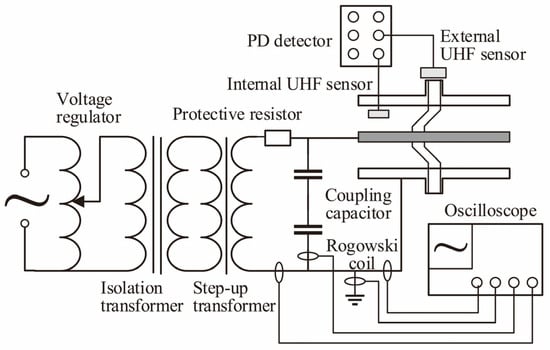
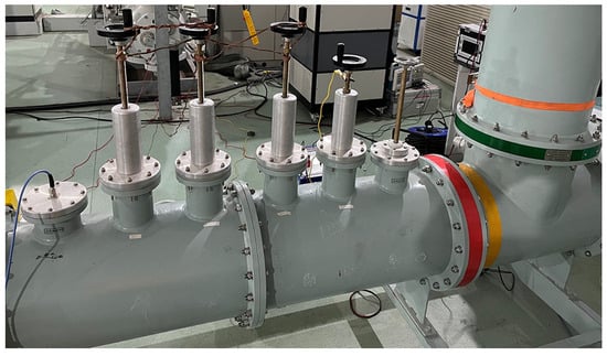
Figure 1 shows the overall circuit structure of the experimental platform. Figure 2 shows the GIS PD experimental device, which was designed and manufactured based on a 126 kV GIS prototype. The two gas chambers on the right house a step-up transformer and a coupling capacitor, respectively. The left gas chamber is used to install the electrodes for generating PD and the sensors for detecting PD signals. Electrodes are installed at the bottom ends of the four adjustment rods in the middle.

Figure 1. Overall circuit structure of the experimental platform.

Figure 2. The GIS PD experimental device.

2.1.2. Electrode Structures for Simulating PD

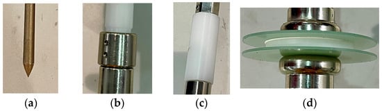
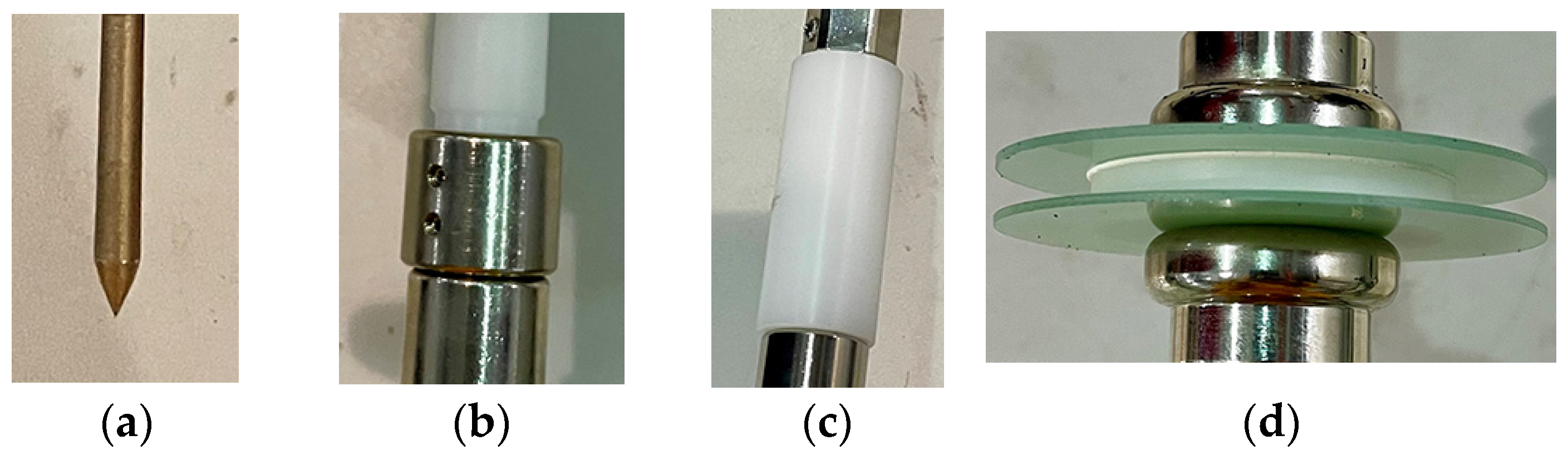
Four types of PD were simulated by configuring discharge electrodes in the GIS PD experimental device. The four discharge electrodes used in the experiment are shown in Figure 3.

Figure 3. Discharge electrodes: (a) Type P; (b) Type F; (c) Type V; (d) Type S.

The Type P electrode in Figure 3a is made of copper, with a conductor diameter of 6 mm and a tip length of 10 mm. During the experiment, the conductor tip was positioned 3 mm from the GIS high-voltage busbar.

The Type F electrode shown in Figure 3b consists of an upper cylindrical resin and two lower conductors. There is a 2 mm gap between the two conductors. The upper conductor is 20 mm high with an outer diameter of 25 mm and an inner diameter of 15 mm. The lower conductor is 20 mm high. During the experiment, the lower conductor maintained good contact with the GIS high-voltage busbar, while the middle conductor served as the floating conductor.

The Type V electrode shown in Figure 3c consists of two end conductors and a resin in the middle. A bubble with a diameter of 2 mm was created within the cylindrical resin, which has a height of 54 mm and a diameter of 25 mm.

The Type S electrode shown in Figure 3d consists of two conductors, upper and lower, with the insulating medium sandwiched between them. Both conductors have a diameter of 30 mm. The two green circular disks in the middle are made of rubber medium, each with a diameter of 60 mm and a thickness of 1 mm. Sandwiched between the two disks is an annular epoxy resin, with a height of 5 mm, an outer diameter of 40 mm, and an inner diameter of 15 mm.

The discharge behavior of each electrode was verified through specialized discharge testing to ensure it met the design objective of confining discharge to target locations with minimal occurrence elsewhere. The testing used an FDC-UV300 UV imaging camera, compliant with the IEC 62478 standard [26], manufactured by Fudichen, Beijing, China.

2.1.3. Measurement Devices

A Rogowski coil was used to measure the discharge current. Since the output voltage of the Rogowski coil is measured directly using an oscilloscope, the design goal is to obtain a voltage of several hundred millivolts under discharge current. To achieve this, the Rogowski coil was designed with 50 turns, a ring height of 2 cm, and inner and outer radii of 1.8 cm and 3 cm, respectively. Calculations show that its inductance is 70 microhenries. The signal was recorded using a DPO3034 oscilloscope manufactured by Tektronix, Shanghai, China. The oscilloscope has a bandwidth of 300 MHz and a sampling rate of 2.5 GS/s

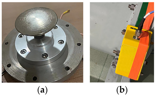
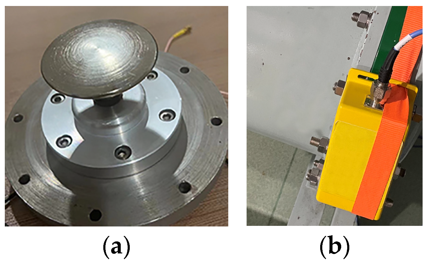
The UHF method utilized two UHF sensors installed inside or outside the GIS, as shown in Figure 4. These two UHF sensors have a detection bandwidth of 300–1500 MHz and an effective height of ≥13 mm. The internal UHF sensor was installed in the leftmost hole shown in Figure 2, and the external UHF sensor was installed at the pouring hole of the basin insulator. The UHF sensors transmitted signals to the PD71 PD detector manufactured by SDMT, Shanghai, China. The PD detector has a detection bandwidth of 100–2000 MHz and a signal sampling rate of 100 MS/s.

Figure 4. UHF sensors: (a) internal UHF sensor; (b) external UHF sensor.

2.2. Results of PD Experiments

The experimental results comprise the waveforms acquired by the oscilloscope and the discharge pulse sequences acquired by the PD detector.

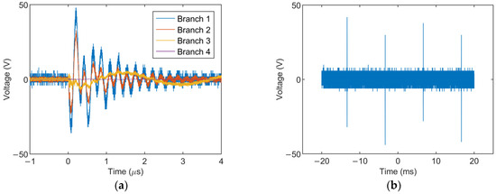
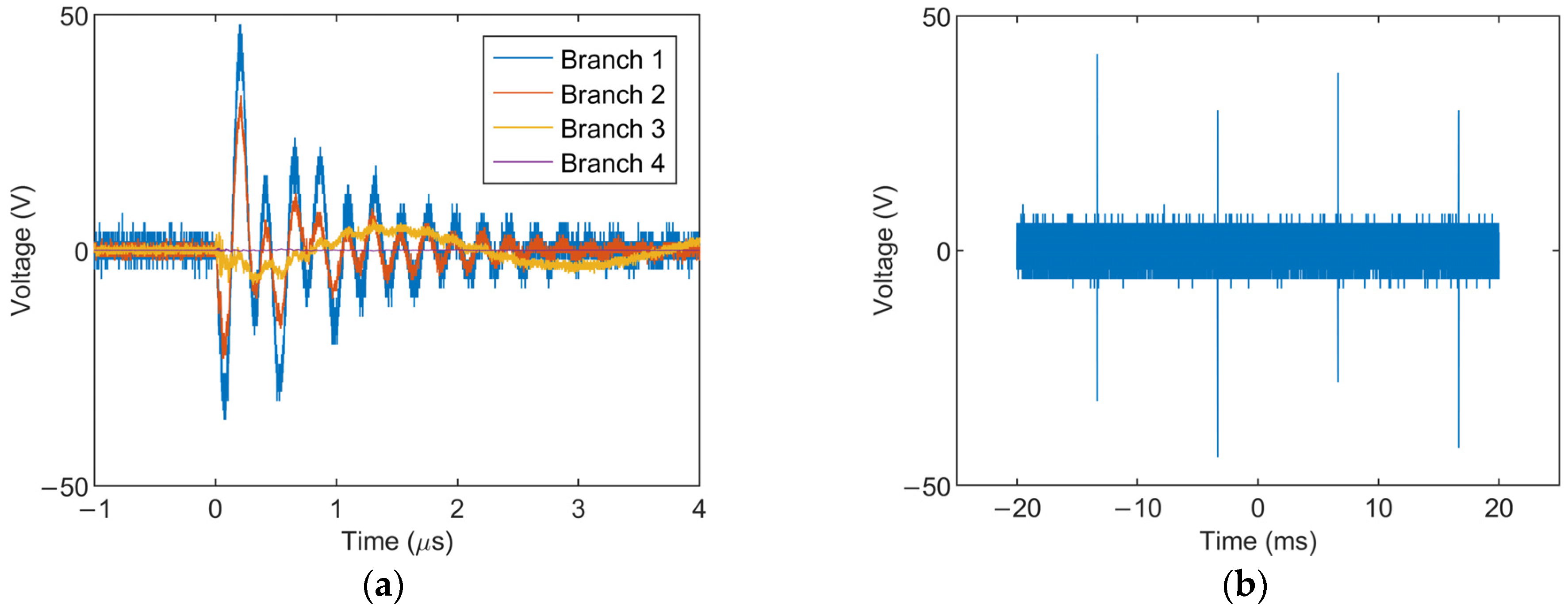
A representative set of waveforms is shown in Figure 5. Over 200 sets of valid waveforms were obtained, with each set comprising both the waveform of a single pulse and the waveform measured during two power frequency cycles.

Figure 5. A set of waveforms collected in the experiment: (a) the waveform of a single pulse measured at the GIS shell grounding (branch 1), coupling capacitor grounding (branch 2), step-up transformer secondary side grounding (branch 3), and single-point grounding wire (branch 4); (b) the waveform measured at branch 1 during two power frequency cycles.

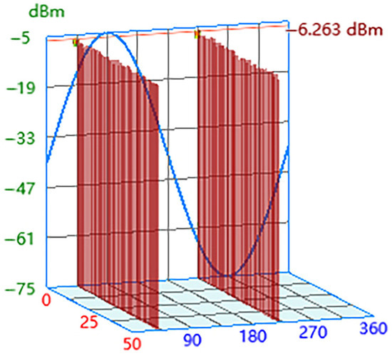
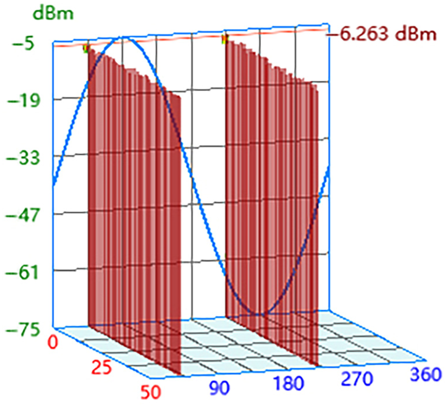
Each discharge pulse sequence is represented by a data matrix with dimensions of 50 rows by 256 columns, where each row represents one power frequency cycle and each column corresponds to a phase point. It should be noted that a phase point here represents a small phase interval. Matrix elements denote the amplitude of discharge pulses, with null values indicating no discharge pulses. The data matrix is visualized as a PRPS graph in Figure 6.

Figure 6. The PRPS graph of a PD pulse sequence acquired by the UHF method. In the graph, the red bars represent discharge pulses, the x-axis represents the power frequency cycle number, the y-axis represents the pulse phase, and the z-axis represents the pulse amplitude. The blue curve represents the power frequency reference waveform.

3. Definition and Extraction of Features for PD Signals Based on Histograms

Signals of different PD types contain different information, and the information needs to be represented by features. To classify PD types based on signals, it is essential to define signal features appropriately. The feature definition method directly affects the separability between different PD types and the effectiveness of subsequent PD type recognition. When defining signal features, it is important to balance the representational capability of the features with the computational complexity of the extraction algorithm.

3.1. Feature Definitions

3.1.1. DCPH

The discharge count at each power frequency phase point provides important information about PD signals. Considering the randomness of discharges, the total number of discharge pulses at the same phase point across several consecutive cycles can serve as a feature of PD signals. The phase point here represents a small interval $\left[{\alpha }_1,{\alpha }_1+\Delta \alpha \right]$. Therefore, the DCPH refers to the discharge count within each interval across n consecutive cycles. The size of the interval $\Delta \alpha$ affects both the number and the height of the bins in the histogram. The lower limit of $\Delta \alpha$ is determined by the pulse resolution capability of the PD measurement instrument. The selection of $\Delta \alpha$ will be discussed in Section 4.2.2. Each histogram consists of m bins ($\Delta \alpha =360/m$). The height values of these bins form an m-dimensional vector ${\mathit{H}}_{\mathrm{P}}=\left[h_1,h_2,\dots ,h_i,\dots ,h_m\right]$, where $h_i$ represents the discharge count in the i-th interval.

3.1.2. DCAH

The amplitude of the PD pulse also provides important information about PD signals. The DCAH is defined as the total number of discharge pulses at different amplitudes across n consecutive power frequency cycles. Since the amplitude of the discharge pulse is related to the applied voltage and the electrode geometry, the normalization of pulse amplitudes is necessary. The normalization method linearly scales the amplitudes of all PD pulses measured across n consecutive cycles to the range $\left[0, 1\right]$, such that the minimum and maximum amplitudes are mapped to 0 and 1, respectively. Consequently, the amplitudes in the DCAH are normalized values. The DCAH can also be represented as a vector ${\mathit{H}}_{\mathrm{A}}=\left[h_1,h_2,\dots ,h_i,\dots ,h_l\right]$, where l denotes the number of bins in the histogram. Thus, the bin width is $1/l$, and $h_i$ represents the discharge count in the i-th interval.

Within a power frequency cycle, PD pulses can generally be divided into two groups based on their occurrence in the positive or negative half-cycle. An exception is the Type V PD, which may occur before the voltage zero-crossing point. For this exception, the two groups can still be divided by appropriately shifting the division point leftward. Since the two pulse groups have different amplitude ranges, they must be processed separately. Each group is therefore represented by a distinct DCAH.

3.2. Formation of the Two Histogram-Based Feature Vectors

The measured PD signals primarily consist of discharge pulse sequences acquired by the PD detector and discharge pulse currents obtained by current measurement. First, the discharge pulses within each signal were correlated with the power frequency phase to construct a pulse information matrix:

$$\mathit{G}=\left[\left[{\phi }_1,A_1\right],\left[{\phi }_2,A_2\right],\dots ,\left[{\phi }_i,A_i\right],\dots ,\left[{\phi }_N,A_N\right]\right]$$

(1)

where ${\phi }_i$ is the power frequency phase corresponding to the i-th pulse, $A_i$ is the amplitude of the i-th pulse, and N denotes the total number of pulses within the signal.

Based on the pulse information matrix G, the two histogram-based feature vectors can be easily formed. Following the selection of $\Delta \alpha$, the DCPH vector was constructed by assigning all pulses from G into histogram bins based on their corresponding ${\phi }_i$. To form the DCAH vector, the pulses within each signal were first divided into two groups. For each group, the amplitudes were normalized using the maximum and minimum amplitudes of that group. Following the selection of l, the DCAH vector was constructed by assigning all pulses from G into histogram bins according to their normalized amplitudes.

3.3. Typical Histogram-Based Features of Four PD Types

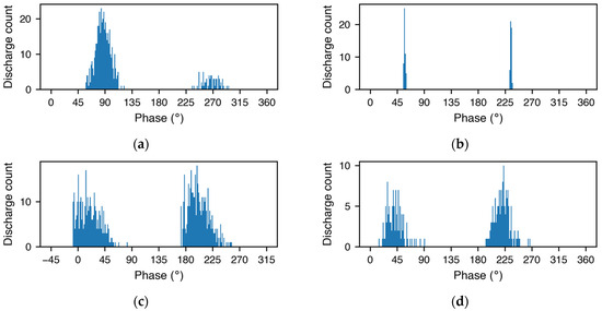
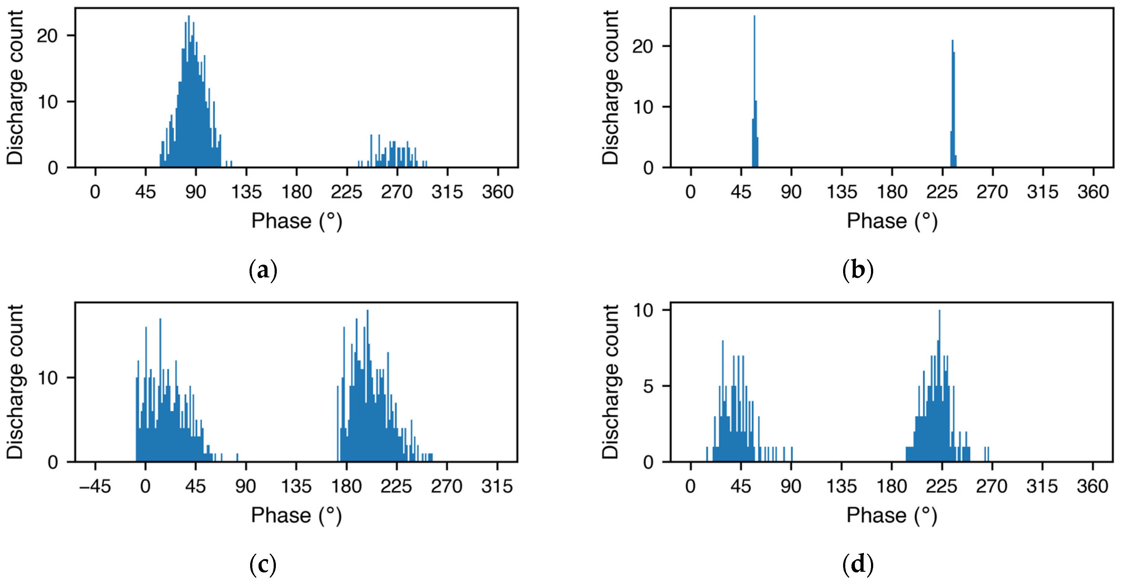
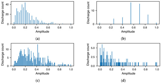
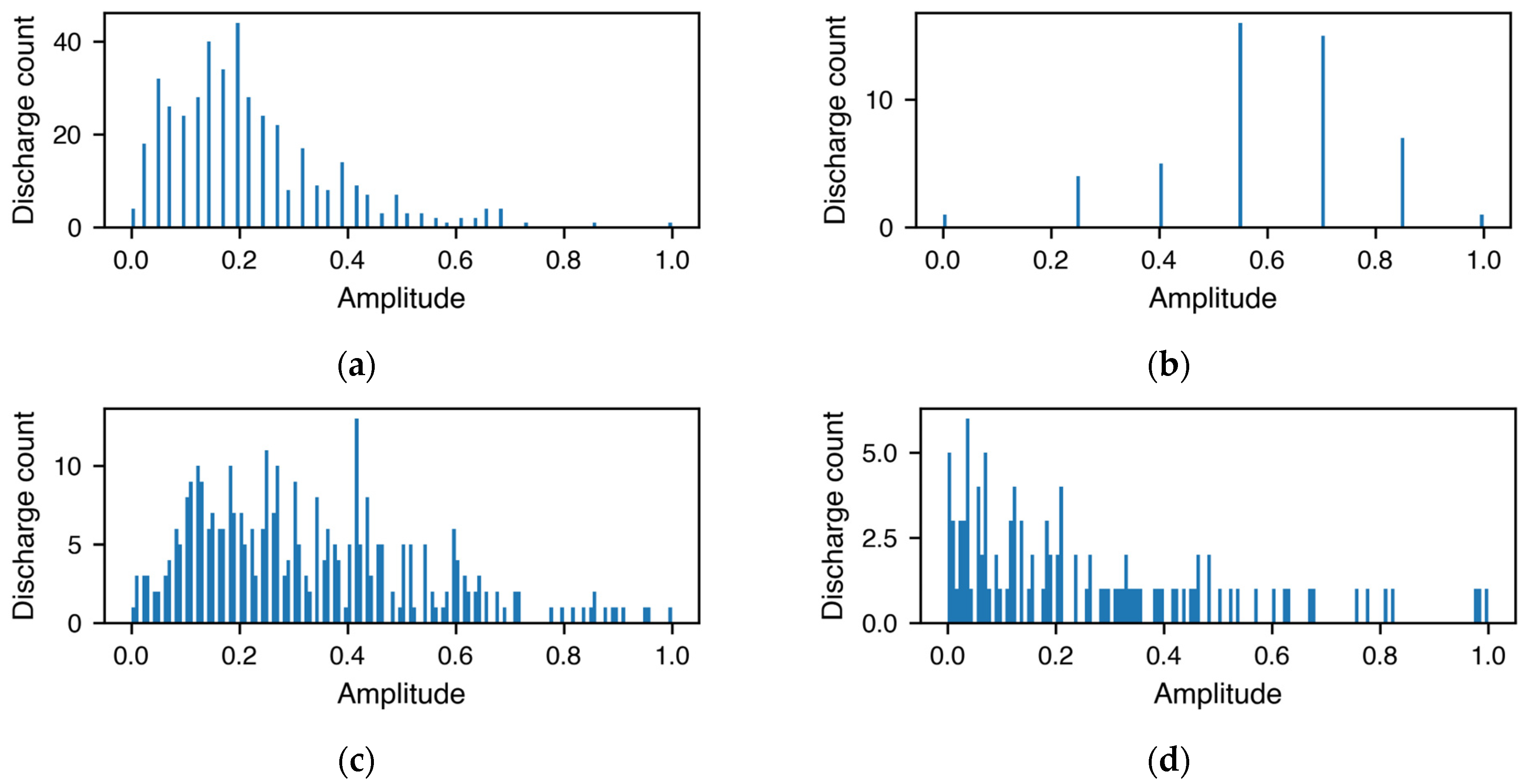
Typical histogram-based features of the four PD types were extracted from experimental results. Figure 7 shows typical DCPHs of the four PD types ($\Delta \alpha =1.4°$). Figure 7 reveals that the phase distribution of Type P differs most significantly between half-cycles. Type F has the narrowest phase distribution in both half-cycles. Type V is the only type with discharges occurring before the voltage zero-crossing point. Among all four types, Types P and F exhibit the most pronounced DCPH characteristics. However, Type V PD may not occur before the voltage zero-crossing point if space charge accumulation is insufficient. Under these conditions, the phase distributions of Types V and S can overlap, making their histogram differences less distinct. Figure 8 shows typical DCAHs of the four PD types ($l=150$). Figure 8 indicates that the amplitude distribution of Type P is concentrated around 0.2, with a low proportion of pulses observed in $\left[0.5,1.0\right]$. The amplitudes of Type F take values only at a few discrete points. The amplitudes of Type V are primarily distributed in $\left[0,0.7\right]$ and are relatively dispersed within this range. The amplitudes of Type S are primarily distributed in $\left[0,0.2\right]$. Consequently, Type F exhibits the most distinct DCAH characteristics, while the other three types can be differentiated by their primary amplitude distribution ranges and dispersion levels.

Figure 7. Typical DCPHs: (a) Type P; (b) Type F; (c) Type V; (d) Type S.

Figure 8. Typical DCAHs: (a) Type P; (b) Type F; (c) Type V; (d) Type S.

4. A Recognition Method for PD Types Based on Histogram Distance and Its Performance

The distributions of DCPH and DCAH for the four PD types are analyzed using the histogram distance. The analysis results show that histograms of different PD types cluster in distinct regions in the feature space, indicating that the two features can distinguish the different PD types. To leverage the complementary advantages of the two features, a distance-level feature fusion method based on histogram distance is proposed. Then, a distance-based KNN classifier is used to recognize PD types. The effectiveness of the proposed features and recognition method is verified through comparative and feature-ablation experiments.

4.1. Distributions of Histogram-Based Features for the Four PD Types

The DCPHs extracted from experimental PD data formed a feature space. Each DCPH was represented as a point within the space. By defining a histogram distance metric, the distribution of these points within the space can be used to analyze the distribution of DCPHs for the four types of PD. This same process can also be applied to the extracted DCAHs.

The distribution of points within the space is directly influenced by the choice of the histogram distance metric. A variety of distance metrics for histograms have been extensively studied, including commonly used measures such as Euclidean distance, histogram intersection, and Hellinger distance [27,28]. Let two histograms ${\mathit{H}}_1=\left[x_1,x_2,\dots ,x_N\right]$ and ${\mathit{H}}_2=\left[y_1,y_2,\dots ,y_N\right]$, where ${\displaystyle {\sum }_{i=1}^N{x}_i}={\displaystyle {\sum }_{i=1}^N{y}_i}=1$. The Euclidean distance, histogram intersection, and Hellinger distance between two histograms are calculated as:

$$d_{\mathrm{ED}}\left({\mathit{H}}_1,{\mathit{H}}_2\right)=\sqrt{{\displaystyle {\sum }_{i=1}^N{\left(x_i-y_i\right)}^2}}$$

(2)

$$d_{\mathrm{ID}}\left({\mathit{H}}_1,{\mathit{H}}_2\right)=1-{\displaystyle {\sum }_{i=1}^N\min \left(x_i,y_i\right)}$$

(3)

$$d_{\mathrm{HD}}\left({\mathit{H}}_1,{\mathit{H}}_2\right)=\sqrt{1-{\displaystyle {\sum }_{i=1}^N\sqrt{x_i{y}_i}}}$$

(4)

To visually analyze the distribution of points within the feature space, multidimensional scaling (MDS) was employed to project these points onto a two-dimensional plane. MDS aims to maintain the distances between points in the original space, such that the Euclidean distances between points in the two-dimensional plane closely approximate those distances [29]. Thus, the distribution of points on the two-dimensional plane can provide a reliable representation of their distribution in the original space.

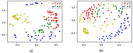
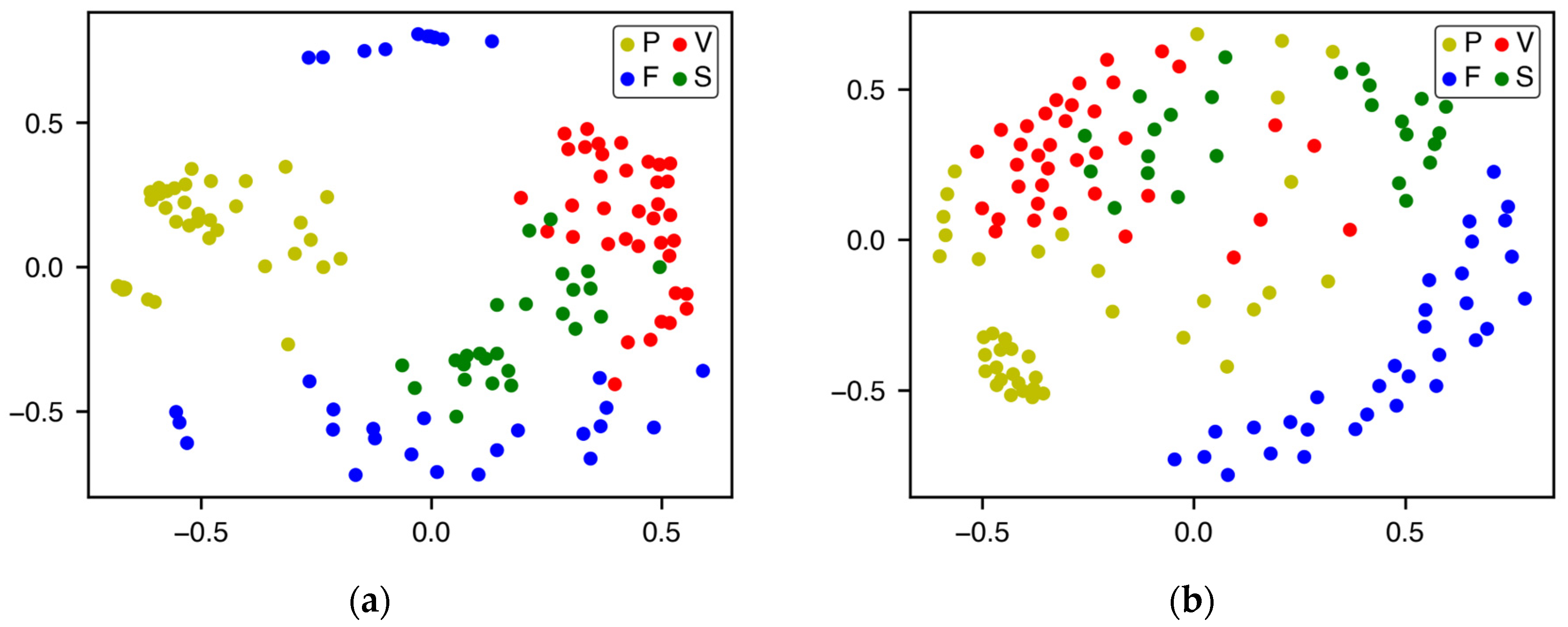
Figure 9 shows the distributions of the two histogram-based features for the four PD types on the two-dimensional plane, using MDS with the distance metric being the histogram intersection. Each point in the figure represents a histogram, with its color denoting the PD type it belongs to. As shown in Figure 9a, the DCPHs of different PD types are located within distinct regions, indicating that the DCPH can distinguish the different PD types. In Figure 9b, a clear boundary separates Type F from the other three types, whereas the regions of the latter three types exhibit overlap. This indicates that the DCAH is more effective than the DCPH at distinguishing Type F but less effective at discriminating among the other three types.

Figure 9. Distributions of the two features for the four PD types: (a) DCPH; (b) DCAH.

4.2. Recognition Method for PD Types

4.2.1. Methodology and Process

To leverage the complementary advantages of both the DCPH and the DCAH, we defined a fused distance metric which is calculated as the weighted average of their individual distances. Since the pulses in each PD sample are divided into two groups, each yielding its own DCAH, each sample is represented by one DCPH and two DCAHs. The distances computed using these two DCAHs are assigned equal weights. The fused distance metric $d_{\mathrm{fused}}$ is calculated as:

$$d_{\mathrm{fused}}=w\cdot d_{\mathrm{P}}+\left(1-w\right)\cdot \left(d_{\mathrm{A}1}+d_{\mathrm{A}2}\right)/2$$

(5)

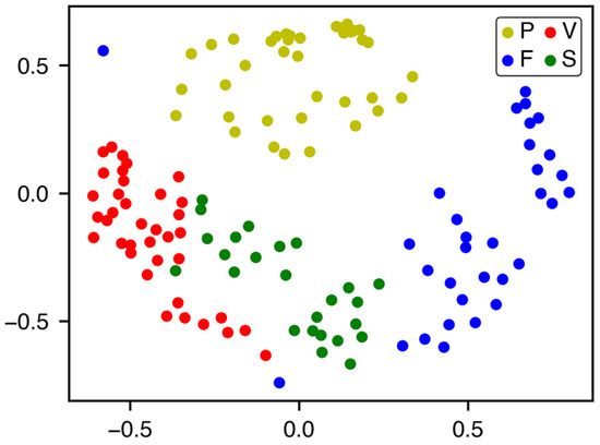
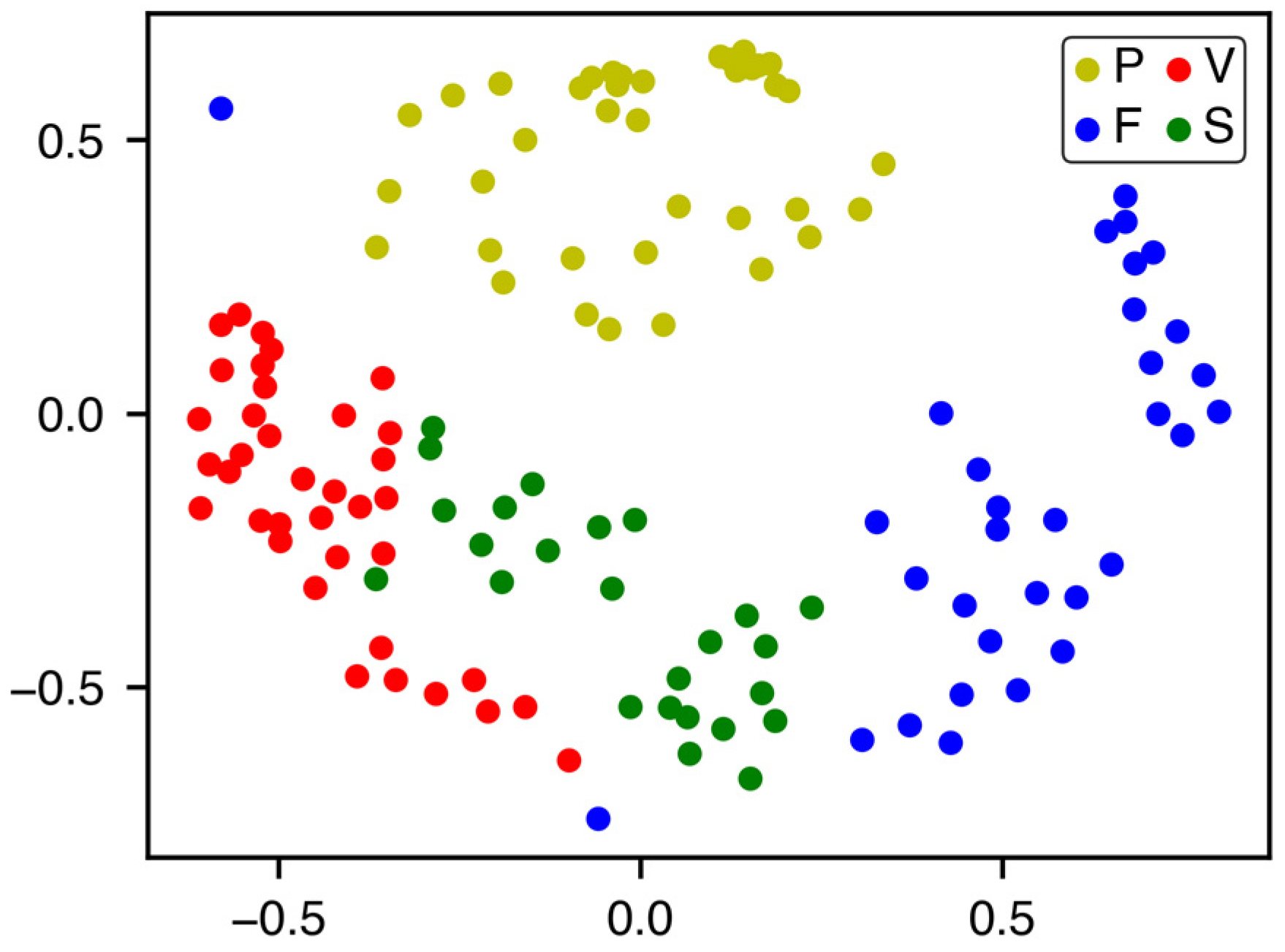
where $d_{\mathrm{P}}$ is the distance computed using the DCPH, while $d_{\mathrm{A}1}$ and $d_{\mathrm{A}2}$ are the distances computed using the DCAHs of the first and second pulse groups, respectively. The weighting coefficient w governs the relative contribution of each feature to the fused distance. When w is set to 0.5, Figure 10 shows the distribution of samples for the four PD types based on the fused distance, using MDS with the histogram intersection. In comparison to Figure 9, the separability of the four PD types is markedly enhanced, which indicates the superior performance of the distance-level feature fusion approach over using any single feature.

Figure 10. The distribution of samples for the four PD types after the distance-level feature fusion.

The distributions of the histogram-based features for the four PD types indicate that histograms with closer distances are more likely to belong to the same PD type. Thus, we use the distance-based KNN classifier to recognize PD types. The KNN denote the k closest histograms in the set of histograms with known PD types to the target histogram. By counting the PD types of these k histograms, the PD type with the highest proportion is assigned to the target histogram.

Therefore, the process of the recognition method for PD types based on histogram distance is: (1) extract the DCPH and two DCAHs from the target PD signal; (2) calculate the distance between the target histogram and the corresponding histogram of each signal with known PD types; (3) calculate the fused distance between the target signal and each signal with known PD types, and select the k closest signals to the target signal; (4) count the PD types of these k signals, and assign the most frequent PD type as the recognition result.

4.2.2. Selection Strategy for Parameters in the Method

While a larger number of power frequency cycles provides a longer signal containing more PD information, it also increases computational cost. Furthermore, beyond a certain length, the recognition performance plateaus due to information saturation. Testing using the experimental PD data reveals that recognition performance remains comparable across a range of 30 to 50 cycles. Therefore, it is recommended to set this parameter within this range. In this study, the number of power frequency cycles was set to 50.

While finer histogram binning better captures local details and benefits recognition, the number of bins is limited by the measurement instrument’s resolution for the phase or amplitude of PD signals. It is therefore recommended to set the number of bins to this practical upper limit. In this study, the numbers of bins for the DCPH and DCAH were set to 256 and 150, respectively.

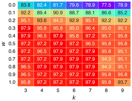
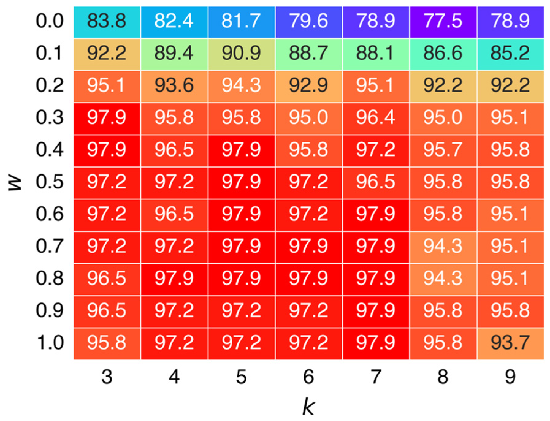
The choice of histogram distance metric and weighting coefficient w affects the fused distance between samples, leading to different distributions of samples in the space. The value of k in the KNN algorithm affects the decision boundary for type recognition. A small k yields a noise-sensitive, complex boundary capable of capturing local patterns, while a large k creates an over-smoothed boundary that ignores local details. The best choice of histogram distance metric, w, and k depends upon the data used. Therefore, cross-validation can be performed on the training data using various possible parameter combinations to select the one that yields the best recognition performance. To illustrate the impact of k and w on the model’s recognition performance, we plotted the cross-validation results as a heatmap, as shown in Figure 11. Each element in Figure 11 represents the average accuracy of the four-fold cross-validation under the corresponding parameter combination.

Figure 11. Recognition accuracy under different k and w.

4.3. Experimental Results

4.3.1. Experimental Setup

To evaluate the effectiveness of the PD type recognition method, we utilized the PD signals measured in Section 2.2 as the dataset for training and testing. The dataset was divided into training and test sets with a 3:1 ratio. Four-fold cross-validation was performed on the training set to select the parameter combination yielding the highest recognition accuracy. This selected parameter set was then used to train the model on the entire training set. Finally, the test set was used to evaluate the recognition accuracy of the method for the four PD types.

4.3.2. Comparison of Different Feature Fusion Methods

To validate that the proposed feature fusion method can achieve good recognition performance, PD type recognition accuracy was compared across different feature fusion methods. The comparison evaluated feature concatenation versus the proposed distance-level fusion method. For feature concatenation, three classifiers—KNN, SVM, and GBDT—were employed for PD type recognition. For distance-level fusion, KNN was used for recognition under three histogram distance metrics. The comparison results are shown in Table 1. In Table 1, both FC-KNN and ED-KNN use Euclidean distance, while ED-KNN’s recognition accuracy is 10.4% higher than FC-KNN, confirming the effectiveness of the proposed distance-level fusion method. The recognition performance of the distance-level fusion method is significantly influenced by the chosen distance metric. The best accuracy of 95.8% is achieved when using the intersection distance.

Table 1. Recognition accuracy of different feature fusion methods.

Methods	Accuracy (%)
	P	F	V	S	Total
FC-KNN	92.9	27.3	100	81.8	77.1
FC-SVM	100	90.9	83.3	90.9	91.7
FC-GBDT	100	90.9	91.7	90.9	93.8
ED-KNN	100	63.6	91.7	90.9	87.5
HD-KNN	100	81.8	100	90.9	93.8
ID-KNN	100	90.9	100	90.9	95.8

FC: feature concatenation; ED: Euclidean distance; HD: Hellinger distance; ID: intersection distance.

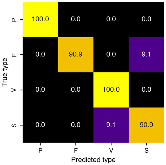
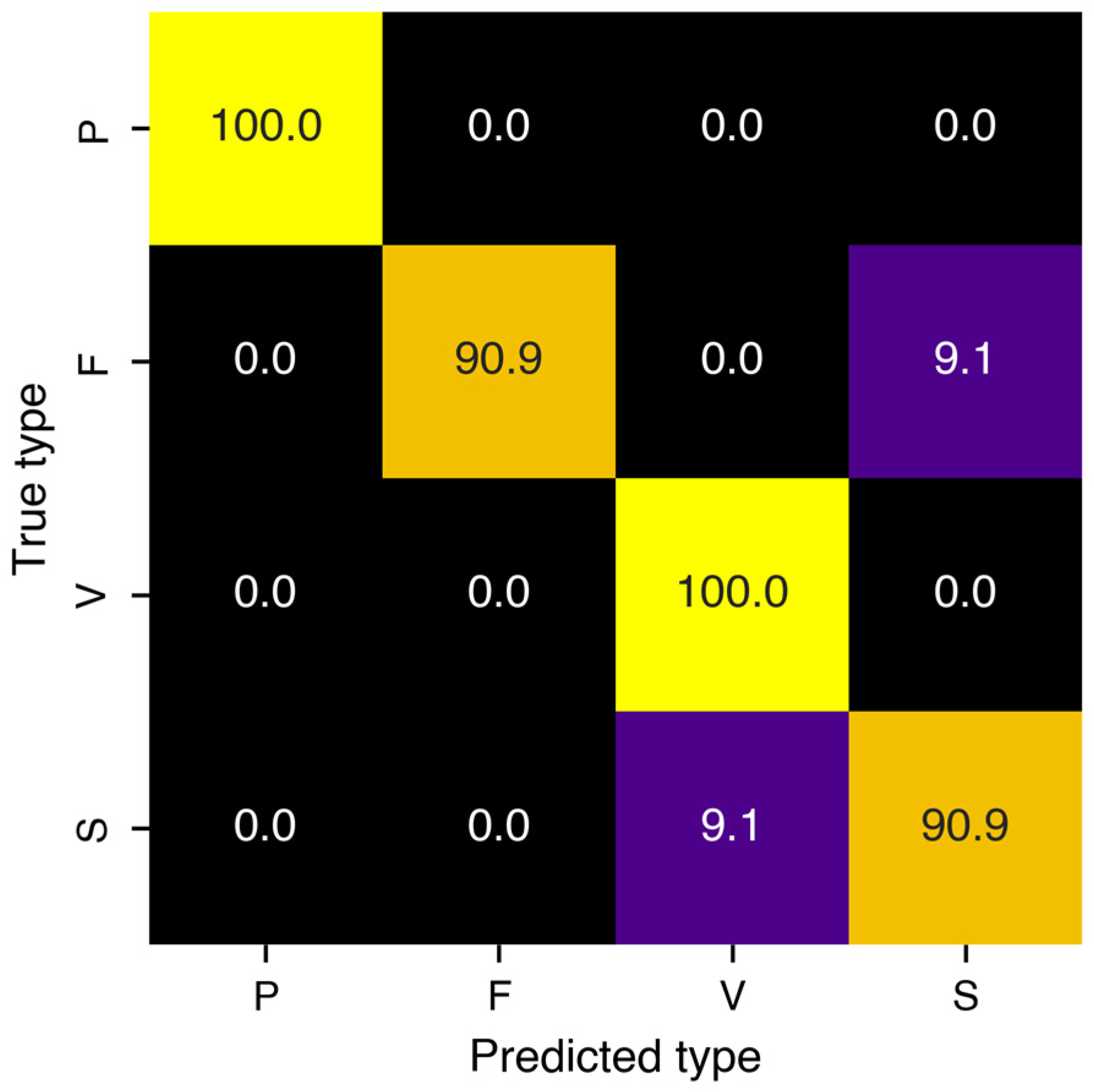
To further evaluate the recognition performance of ID-KNN, we calculated its precision, recall, and F1-score on the test set, as shown in Table 2. The average values of the three metrics in Table 2 were calculated using the macro formula. As shown in Table 2, ID-KNN can accurately identify Type P, but there is confusion among the other three types. To illustrate the recognition performance of ID-KNN more intuitively, the confusion matrix of the test results is plotted in Figure 12.

Table 2. The precision, recall, and F1-score of ID-KNN.

Metrics	P	F	V	S	Average
Precision (%)	100	100	92.3	90.9	95.8
Recall (%)	100	90.9	100	90.9	95.5
F1-score (%)	100	95.2	96.0	90.9	95.5

Figure 12. The confusion matrix of ID-KNN. A Brighter color indicate a higher value.

4.3.3. Feature Ablation Experiment

To investigate the contribution of the two proposed features and their fusion method to PD type recognition, feature ablation was conducted to compare the recognition accuracy of using DCPH or DCAH alone with that after feature fusion. Intersection distance was employed as the distance metric in all three cases, with KNN serving as the classifier. The comparison results are shown in Table 3. As Table 3 indicates, the overall recognition accuracy after feature fusion improved by 12.5% and 6.2% compared to using DCAH and DCPH alone, respectively, confirming the necessity of feature fusion. Table 3 also demonstrates that DCAH and DCPH exhibit complementary recognition capabilities for Type P and Type F. This complementary advantage underlies the enhanced recognition accuracy achieved through feature fusion.

Table 3. Feature ablation results.

Features	Accuracy (%)
	P	F	V	S	Total
DCAH	71.4	100	83.3	81.8	83.3
DCPH	100	72.7	91.7	90.9	89.6
Fused	100	90.9	100	90.9	95.8

4.3.4. Comparison of Different Recognition Methods

To verify the advantages of the proposed PD type recognition method, we compared it with existing approaches: the statistical feature-based recognition method (SF-RF) [14] and the HOG feature-based recognition method (HOG-GBDT) [17]. SF-RF uses the PD pulse count ratios in every 30-degree phase interval, along with the kurtosis and skewness of both positive and negative polarity half-cycles, as features extracted from the PRPD spectra. It then uses a random forest to recognize PD types. HOG-GBDT extracts HOG features from the PRPD grayscale image and subsequently uses GBDT for PD type recognition.

The hyperparameters for the three methods were optimized using grid search with 4-fold cross-validation on the training set. The results are summarized in Table 4. The recognition performance of the three methods is shown in Table 5. Table 5 demonstrates that our proposed PD type recognition method, ID-KNN, achieves higher recognition accuracy than SF-RF and HOG-GBDT. The time values in Table 5 represent the total duration for feature extraction, training, and testing. ID-KNN and SF-RF exhibit comparable processing times, both of which are significantly shorter than HOG-GBDT. HOG-GBDT requires more computation time due to the high dimensionality of HOG features. Additionally, RF and GBDT require tuning at least three parameters, such as the number of trees, maximum depth, and minimum number of samples required for node splitting. In contrast, KNN requires tuning only one parameter. Therefore, the method proposed in this paper is easy to use, is computationally simple, and achieves excellent recognition accuracy.

Table 4. Hyperparameters used for the three methods.

Methods	Hyperparameters	Value
SF-RF	Number of trees	100
	Maximum depth	2
	Min_samples_split	20
HOG-GBDT	Number of trees	100
	Learning rate	0.2
	Subsample	0.6
	Maximum depth	3
	Min_samples_split	10
ID-KNN	k	3
	w	0.3

Table 5. Recognition performance of different methods.

Methods	Accuracy (%)					Time (s)
	P	F	V	S	Total
SF-RF	100	81.8	83.3	90.9	89.6	0.3
HOG-GBDT	100	100	75.0	90.9	91.7	8.4
ID-KNN	100	90.9	100	90.9	95.8	0.3

4.3.5. Noise Injection and Robustness Evaluation

To augment the dataset and evaluate the robustness of the proposed method against noise, Gaussian white noise was injected into the original PD signals. The noise level is controlled via the signal-to-noise ratio (SNR), calculated as:

$$SNR=10{\log }_{10}\left({\displaystyle \frac{{\displaystyle {\sum }_{i=1}^N{X}^2\left(i\right)}}{{\displaystyle {\sum }_{i=1}^N{Y}^2\left(i\right)}}}\right)$$

(6)

where X(i) represents the original PD signal, Y(i) represents the noise signal, and N is the number of sampling points. By injecting noise, we obtained noisy datasets with SNRs of 20 dB, 10 dB, 5 dB, and −5 dB. For each SNR level, each original PD signal was injected with 5 different Gaussian white noise signals, resulting in 5 noisy signals. Consequently, the total number of samples in the noisy datasets for each SNR is 1000 (200 × 5), with 250 samples for each PD type. To prevent data leakage, the original dataset was divided into training, validation, and test sets in a 12:3:5 ratio. Noise was then injected into each set separately, ensuring that augmented samples of the same original signal appear only within the same set.

The parameters of the proposed ID-KNN recognition method were tuned on the validation set, and then tested using the test set. The accuracy of the ID-KNN method at different SNR levels is shown in Table 6. The results indicate that the proposed ID-KNN method possesses strong noise resistance, with a recognition accuracy remaining above 89% at an SNR of 5 dB. This is because, when noise is low, its impact on the phase and amplitude of PD pulses is minimal, and the proposed features based on phase and amplitude distributions are robust to noise. When the SNR drops to −5 dB, some weak PD pulses are masked by noise or spurious pulses appear, leading to a significant decrease in recognition accuracy. As shown in Table 6, Type F can still be accurately identified even when noise is high. This is because the amplitude of Type F is relatively large, making it less susceptible to noise interference.

Table 6. Recognition accuracy under different SNR.

SNR	Accuracy (%)
	P	F	V	S	Total
20 dB	100	98.4	91.9	88.7	94.8
10 dB	100	100	87.1	82.3	92.4
5 dB	92.1	100	77.4	88.7	89.6
−5 dB	82.5	100	71.0	90.3	86.0

5. Conclusions

Four types of PD can be simulated using the corresponding discharge electrodes on the experimental GIS platform. The measurement results of PD signals comprise discharge pulse sequences acquired by the PD detector and discharge pulse currents obtained by current measurement.

The histogram-based features proposed in this paper—DCPH and DCAH—characterize the phase distribution and amplitude distribution of different PD types, respectively. These two features offer strong representational capabilities and are simple to extract. MDS analysis reveals that the histogram features of different PD types cluster in distinct regions, indicating that the proposed features can distinguish different PD types.

To leverage the complementary advantages of both features, a distance-level feature fusion method based on histogram distance is proposed. KNN is then used to recognize the four PD types using the fused distance. Feature ablation experiments demonstrate that recognition accuracy improves by 6–13% after feature fusion. The distance-level feature fusion method achieves higher recognition accuracy than the feature concatenation method, validating its effectiveness. Compared with two existing PD type recognition methods using statistical features and HOG features, the proposed method demonstrates better performance, with recognition accuracy improvements of 4–6%. Furthermore, the proposed method requires less computation time and fewer parameters to be tuned, thus ensuring good practicality.

Actual field environments are far more complex than laboratory settings. For example, laboratory environments are well-shielded, whereas field environments are subject to significant noise and interference. To evaluate the robustness of the proposed method against noise, we synthesized 1000 noisy samples at different SNR levels by injecting Gaussian white noise. Test results on the noisy dataset indicate that our method maintains recognition accuracy above 89% at an SNR of 5 dB, demonstrating strong noise resistance. Moreover, a small amount of random pulse interference has little impact on the phase and amplitude distributions of PD pulses. Therefore, our features based on these distributions are inherently robust to random pulse interference.

Furthermore, our method focuses primarily on discharges from a single PD source, whereas in actual GIS operation, multiple discharge sources may occur simultaneously. One potential improvement is to treat each combination of multiple discharge sources as a distinct type, then extract features and train the model for these types. However, this may lead to potential problems such as a large number of combinations and feature confusion, which will be addressed in our future research.

References

- Li, Z.; Zang, Y.; Wang, C.; Tang, Y.; Ren, T.; Jiang, X. Analysis and Diagnosis of Optical and UHF Partial Discharges in GIS Based on Guided Filtering Fusion. IEEE Trans. Dielectr. Electr. Insul. 2025, 32, 2978–2985. [Google Scholar] [CrossRef] [Scilit]
- Zhu, X.; Hu, C.; Yang, J.; Liu, Z.; Wang, Z.; Liu, Z.; Zang, Y. Acoustic Identification Method of Partial Discharge in GIS Based on Improved MFCC and DBO-RF. Energies 2025, 18, 1619. [Google Scholar] [CrossRef] [Scilit]
- Fan, X.; Qin, W.; Qiu, R.; Zang, Y.; Lu, W.; Zhang, Y.; Chen, R.; Liang, F.; Sun, G.; Luo, H.; et al. A Review of Advanced Acoustic-Chemical-Optical Partial Discharge Monitoring Techniques for Ultra-High-Voltage Gas-Insulated Equipment. High Volt. 2025, 10, 787–806. [Google Scholar] [CrossRef] [Scilit]
- Li, Z.; Qian, Y.; Zang, Y.; Zhao, J.; Sheng, G.; Jiang, X. Optical Partial Discharge Detection and Diagnosis Method Based on PHOG Features. IEEE Trans. Dielectr. Electr. Insul. 2024, 31, 3040–3048. [Google Scholar] [CrossRef] [Scilit]
- Yao, R.; Li, J.; Hui, M.; Bai, L.; Wu, Q. Pattern Recognition for Partial Discharge Using Multi-Feature Combination Adaptive Boost Classification Model. IEEE Access 2021, 9, 48873–48883. [Google Scholar] [CrossRef] [Scilit]
- Xu, Z.; Xu, H.; Yuan, C.; Chen, S.; Chen, Y. Recognition of Partial Discharge in GIS Based on Image Feature Fusion. AIMS Energy 2024, 12, 1096–1112. [Google Scholar] [CrossRef] [Scilit]
- Wu, Y.; Ding, D.; Wang, Y.; Zhou, C.; Lu, H.; Zhang, X. Defect Recognition and Condition Assessment of Epoxy Insulators in Gas Insulated Switchgear Based on Multi-Information Fusion. Measurement 2022, 190, 110701. [Google Scholar] [CrossRef] [Scilit]
- Lee, G.-Y.; Kil, G.-S. Insulation Defect Diagnosis Using a Random Forest Algorithm with Optimized Feature Selection in a Gas-Insulated Line Breaker. Electronics 2025, 14, 1940. [Google Scholar] [CrossRef] [Scilit]
- Saad, M.H.; Hashima, S.; Omar, A.I.; Fouda, M.M.; Said, A. Deep Learning Approach for Cable Partial Discharge Pattern Identification. Electr. Eng. 2025, 107, 1525–1540. [Google Scholar] [CrossRef] [Scilit]
- Zheng, J.; Chen, Z.; Wang, Q.; Qiang, H.; Xu, W. GIS Partial Discharge Pattern Recognition Based on Time-Frequency Features and Improved Convolutional Neural Network. Energies 2022, 15, 7372. [Google Scholar] [CrossRef] [Scilit]
- Bin, F.; Wang, F.; Sun, Q.; Chen, S.; Fan, J.; Ye, H. Identification of Ultra-High-Frequency PD Signals in Gas-Insulated Switchgear Based on Moment Features Considering Electromagnetic Mode. High Volt. 2020, 5, 688–696. [Google Scholar] [CrossRef] [Scilit]
- Gao, W.; Ding, D.; Liu, W. Research on the Typical Partial Discharge Using the UHF Detection Method for GIS. IEEE Trans. Power Deliv. 2011, 26, 2621–2629. [Google Scholar] [CrossRef] [Scilit]
- Jiang, T.; Chen, L.; Yuan, H.; Tan, S.; Xie, H.; Bi, M.; Chen, X. APSO-SVM Based Approach for Partial Discharge Pattern Recognition in Converter Transformer. J. Electr. Eng. Technol. 2026, 21, 1227–1241. [Google Scholar] [CrossRef] [Scilit]
- Lee, G.-Y.; Kil, G.-S.; Kim, S.-W. Partial Discharge Defect Classification in Cast-Resin Transformers Using Machine Learning-Based Algorithms. J. Electr. Eng. 2025, 76, 565–573. [Google Scholar] [CrossRef] [Scilit]
- Sun, S.; Sun, Y.; Xu, G.; Zhang, L.; Hu, Y.; Liu, P. Partial Discharge Pattern Recognition of Transformers Based on the Gray-Level Co-Occurrence Matrix of Optimal Parameters. IEEE Access 2021, 9, 102422–102432. [Google Scholar] [CrossRef] [Scilit]
- Fei, Z.; Li, Y.; Yang, S. Partial Discharge Pattern Recognition Based on an Ensembled Simple Convolutional Neural Network and a Quadratic Support Vector Machine. Energies 2024, 17, 2443. [Google Scholar] [CrossRef] [Scilit]
- Tharamal, L.; Surlekar, S.; Preetha, P.; Haque, N. A New Method for Incipient Fault Diagnosis of Power Transformers Based on Image Processing of Phase Resolved Partial Discharge Pattern of Transformer Oil. Measurement 2026, 258, 119536. [Google Scholar] [CrossRef] [Scilit]
- Dutta, S.; Chen, S.; Illias, H.A. Enhancing Partial Discharge Classification Through Augmented Fault Data Balancing. IEEE Trans. Dielectr. Electr. Insul. 2025, 32, 2948–2957. [Google Scholar] [CrossRef] [Scilit]
- Gueraichi, M.; Nacer, A.; Dhahbi-Megriche, N.; Aliouat, S.; Moulai, H. Discriminative Analysis of HVDC Discharges Over Composite Insulators by Feature Selection Combined with SVM. IEEE Trans. Dielectr. Electr. Insul. 2025, 32, 2888–2895. [Google Scholar] [CrossRef] [Scilit]
- Pradeep, L.; Haque, N.; Preetha, P. Discrimination of Multiple Partial Discharge Sources in Oil Impregnated Pressboard Insulation Using HFCT Sensor & Ensembled Learning Classifiers. Measurement 2025, 254, 117920. [Google Scholar] [CrossRef] [Scilit]
- Sahoo, R.; Karmakar, S. Comparative Analysis of Machine Learning and Deep Learning Techniques on Classification of Artificially Created Partial Discharge Signal. Measurement 2024, 235, 114947. [Google Scholar] [CrossRef] [Scilit]
- Mansour, D.-E.A.; Taha, I.B.M.; Farade, R.A.; Wahab, N.I.B.A. Partial Discharge Diagnosis in GIS Based on Pulse Sequence Features and Optimized Machine Learning Classification Techniques. Electr. Power Syst. Res. 2022, 211, 108162. [Google Scholar] [CrossRef] [Scilit]
- Zheng, Q.; Wang, R.; Tian, X.; Yu, Z.; Wang, H.; Elhanashi, A.; Saponara, S. A Real-Time Transformer Discharge Pattern Recognition Method Based on CNN-LSTM Driven by Few-Shot Learning. Electr. Power Syst. Res. 2023, 219, 109241. [Google Scholar] [CrossRef] [Scilit]
- Chang, C.-K.; Lin, Y.-H. Defect Recognition for Partial Discharge Patterns of Gas Insulated Switchgear and Cable Joint Based on Deep Learning Methods. IEEE Trans. Dielectr. Electr. Insul. 2025, 32, 1147–1154. [Google Scholar] [CrossRef] [Scilit]
- Wang, Y.; Yan, J.; Yang, Z.; Jing, Q.; Qi, Z.; Wang, J.; Geng, Y. A Domain Adaptive Deep Transfer Learning Method for Gas-Insulated Switchgear Partial Discharge Diagnosis. IEEE Trans. Power Deliv. 2022, 37, 2514–2523. [Google Scholar] [CrossRef] [Scilit]
- IEC 62478 Standard; High Voltage Test Techniques—Measurement of Partial Discharges by Electromagnetic and Acoustic Methods. International Electrotechnical Commission: Geneva, Switzerland, 2016.
- Cha, S.-H.; Srihari, S.N. On Measuring the Distance between Histograms. Pattern Recognit. 2002, 35, 1355–1370. [Google Scholar] [CrossRef] [Scilit]
- Li, W.; Ding, W.; Sadasivam, R.; Cui, X.; Chen, P. His-GAN: A Histogram-Based GAN Model to Improve Data Generation Quality. Neural Netw. 2019, 119, 31–45. [Google Scholar] [CrossRef] [Scilit]
- Cox, T.; Cox, M. Multidimensional Scaling, 2nd ed.; Chapman and Hall/CRC: New York, NY, USA, 2000. [Google Scholar]
Disclaimer/Publisher’s Note: The statements, opinions and data contained in all publications are solely those of the individual author(s) and contributor(s) and not of MDPI and/or the editor(s). MDPI and/or the editor(s) disclaim responsibility for any injury to people or property resulting from any ideas, methods, instructions or products referred to in the content. |
© 2026 by the authors. Licensee MDPI, Basel, Switzerland. This article is an open access article distributed under the terms and conditions of the Creative Commons Attribution (CC BY) license.