Development and Verification of CUPID-MSR Using the de Vahl Davis Natural-Convection Benchmark

Abstract

This study provides the first systematic verification of the CUPID-MSR thermal–hydraulic code for molten-salt reactor applications, incorporating temperature-dependent thermophysical properties of two chloride-based molten salts, KCl–UCl₃ and NaCl–MgCl₂–TRUCl₃. Verification against the de Vahl Davis benchmark for Rayleigh numbers ${10}^3$–${10}^6$ shows agreement within 0.4–3.9%, with the simulations accurately reproducing the reference Nusselt numbers, velocity fields, and thermal boundary layers. Additional temperature sensitivity studies confirm stable and accurate predictions using the implemented thermophysical property correlations over a broad temperature range. Furthermore, the applicability of the Boussinesq approximation is assessed by comparing the full variable-density formulation with the Boussinesq formulation, revealing that the approximation remains accurate when the relative density variation is below approximately 10% ($\beta \Delta T\lesssim 0.1$). The obtained threshold is consistent with classical Boussinesq criteria and confirms their relevance for molten-salt flows.

1. Introduction

In recent years, molten-salt reactors (MSRs) have attracted growing attention because they employ liquid fuel and offer enhanced safety characteristics. In these systems, the fissile material is mixed directly into molten salt and circulated through the primary circuit. This contrasts with conventional light-water reactors (LWRs), in which the fuel remains solid. The molten salt operates at temperatures approaching 700 °C, enabling high thermal efficiency and potentially improved economic performance. A key advantage of MSRs is their strong passive safety features. In accident scenarios, the fuel salt can be drained into dedicated tanks, either automatically or through operator action, where the resulting configuration is subcritical and accident progression is halted.

Historically, molten salts were first employed as reactor fuel in the Aircraft Reactor Experiment (ARE), constructed in 1954 at Oak Ridge National Laboratory (ORNL) in the United States [1]. The reactor formed part of a program investigating nuclear propulsion for military aircraft. Although the aircraft propulsion concept was ultimately discontinued, the research led to the development of the Molten-Salt Reactor Experiment (MSRE), which reached first criticality in 1965 [2]. The MSRE operated at a thermal power of $8{\mathrm{MW}}_{\mathrm{th}}$ using a LiF–BeF₂–ZrF₄–UF₄ fuel salt mixture and remained in operation for approximately four and a half years before being shut down in 1969. Despite challenges related to material corrosion, the experiment successfully demonstrated the feasibility of molten salt fuels in nuclear reactor systems. However, MSR development in the United States was halted as attention shifted toward other reactor concepts.

At present, no MSR has yet entered commercial operation. Nevertheless, MSR technology continues to receive considerable attention as a potential alternative to conventional water-cooled reactors. Several international initiatives are currently pursuing the development of MSR concepts, including Terrestrial Energy’s IMSR-400 in Canada [3], Kairos Power’s KP-FHR reactor in the United States [4], and Saltfoss Energy’s Compact Molten-Salt Reactor being developed in Denmark [5]. In South Korea, research efforts are focused on the Korea Molten-Salt Reactor (K-MSR), a concept designed for marine propulsion with a target thermal power of $100{\mathrm{MW}}_{\mathrm{th}}$ [6,7]. In addition, the Korea Atomic Energy Research Institute (KAERI) and Saltfoss Energy signed a Memorandum of Understanding in 2024 to cooperate on further development of MSR technologies [8].

Reactor concepts that rely on coolants other than water introduce unconventional design features and require adapted safety strategies. Because their thermal–hydraulic behavior differs significantly from that of water-cooled reactors, extensive safety assessments are necessary, and these must rely on verified numerical tools. Most existing power plants employ light water as the primary coolant; therefore, commonly used system analysis codes such as RELAP5 [9], CATHARE [10], and MARS [11] were developed specifically for LWR applications. As a result, these codes are not well suited for analyzing MSRs, leaving a gap in available computational tools. To support the analysis of reactor systems employing non-water coolants, KAERI developed the system code GAMMA, which has been applied to several advanced reactor concepts, including MSRs [12,13,14]. Codes of this type are generally classified as system analysis tools, as they describe the primary reactor circuit and its main components using one-dimensional representations.

In LWR cores, coolant channels are arranged axially and the flow proceeds primarily in the vertical direction. Under these conditions, one-dimensional models can provide acceptable accuracy. In MSRs, however, particularly in fast-spectrum designs, the core typically lacks internal structures such as fuel assemblies, control rods, and graphite moderators. In the absence of solid structures that constrain the flow path, radial circulation develops in addition to axial motion, resulting in strong radial mixing within the reactor vessel. These characteristics lead to inherently three-dimensional flow behavior, making system-scale one-dimensional modeling insufficient for accurately capturing MSR core thermal hydraulics.

To address this limitation, the CUPID-MSR code was developed by extending the well-established CUPID thermal–hydraulic code [15,16] to MSR applications. CUPID has been extensively developed and validated for LWR systems and is a multi-dimensional, component-scale thermal–hydraulic solver for transient two-phase flow based on a two-fluid, three-field formulation. Depending on the selected computational resolution, it can be applied in component-scale, porous-media, or full CFD modes. By incorporating thermophysical property models for molten salts, CUPID-MSR enables the application of this proven computational code to MSR systems. This approach allows component-scale, multi-dimensional simulations capable of capturing buoyancy-driven flow and thermal mixing within the reactor core.

At present, the CUPID-MSR implementation includes two chloride-based molten-salt mixtures: potassium chloride–uranium(III) chloride (KCl–UCl₃) and sodium chloride–magnesium chloride–transuranic(III) chloride (NaCl–MgCl₂–TRUCl₃). In MSRs, the liquid fuel circulates through the primary loop and therefore functions both as the coolant and as the carrier of fissile material. This configuration creates strong two-way feedback between neutronic behavior and thermal–hydraulic conditions. As the salt flows through the reactor system, delayed neutron precursors and fission products are transported with the fluid, while temperature variations introduce additional reactivity feedback effects. For this reason, realistic MSR analysis requires the coupling of neutron kinetics and thermal–hydraulic models within a multiphysics simulation framework. The CUPID code already supports multiphysics coupling with a three-dimensional neutron kinetics solver [17]; however, its current use is limited to LWR applications because suitable three-dimensional neutronics tools for MSRs are not yet available. Once such coupling becomes available, CUPID-MSR is expected to provide a useful platform for the design and safety evaluation of advanced MSR systems.

To evaluate the reliability of CUPID-MSR for molten-salt applications, its predictions are compared with results from a well-known benchmark problem. For this purpose, the natural convection cavity problem introduced by de Vahl Davis [18] is used, and the results are analyzed for both molten-salt mixtures.

In addition to code verification, this study examines the applicability of the Boussinesq approximation. Although widely used to simplify buoyancy-driven flow simulations, its validity over large temperature differences has not been systematically assessed for fluids exhibiting strongly temperature-dependent properties. By comparing the full variable-density formulation of CUPID-MSR with the Boussinesq model over a wide range of density variations, a practical applicability criterion is identified in terms of the nondimensional parameter $\beta \Delta T=\Delta \rho /{\rho }_{\mathrm{ref}}$. This parameter therefore represents the magnitude of density variations relative to the reference density and provides a direct measure of the validity of the linear density approximation used in the Boussinesq formulation. The obtained threshold establishes a practical and broadly applicable criterion consistent with classical natural-convection theory.

Although several thermal–hydraulic codes have been developed for nuclear reactor analysis, verification studies focusing on molten-salt systems and buoyancy-driven natural convection remain limited. The present work addresses this gap by providing the first systematic verification of the CUPID-MSR code for molten-salt applications using the well-established de Vahl Davis natural-convection benchmark, together with a quantitative assessment of the applicability of the Boussinesq approximation for fluids with temperature-dependent thermophysical properties.

Section 2 outlines the implementation of molten-salt thermophysical properties in CUPID-MSR. Section 3 presents the code verification using the de Vahl Davis benchmark. Section 4 introduces the assessment of the Boussinesq approximation and discusses its general applicability. The conclusions are summarized in Section 5.

2. Implementation of Molten-Salt Thermophysical Properties

The CUPID-MSR code was developed to extend the CUPID thermal–hydraulic solver for applications involving MSR systems, in which the working fluid is a molten salt rather than light water. Among the candidate fuel salts, two chloride-based mixtures were implemented: KCl–UCl₃ and NaCl–MgCl₂–TRUCl₃. The eutectic temperature of the NaCl–MgCl₂–TRUCl₃ mixture is lower than that of KCl–UCl₃, which simplifies reactor operation.

Each salt mixture is represented using temperature-dependent correlations for the main thermophysical properties, namely density, specific heat capacity, thermal conductivity, and dynamic viscosity. Thermophysical property correlations for molten salts were implemented based on empirical relations commonly reported in molten-salt thermophysical property databases and previous studies [19,20].

2.1. Density Correlation

The density of each salt mixture was calculated using an empirical linear model for the density of its pure components i, expressed as

$${\rho }_i=A_i+B_{i}T,$$

(1)

where $A_i$ and $B_i$ are empirical constants and T denotes temperature. The molar volume contribution of component i in the mixture can be expressed as

$$x_i{V}_i={\displaystyle \frac{x_i{M}_i}{{\rho }_i}},$$

(2)

where $x_i$ and $M_i$ represent the mole fraction and molar mass of component i, respectively, and their product corresponds to the mass contribution of that component. The density of the salt mixture can therefore be written as

$${\rho }_{\mathrm{mix}}={\displaystyle \frac{{\sum }_i{x}_i{M}_i}{{\sum }_i{x}_i{V}_i}}.$$

(3)

From the linear correlations, the following relations were derived for the two implemented salts:

$${\rho }_{{\mathrm{KCl}–\mathrm{UCl}}_3}=3.69\times {10}^3-0.39T,$$

(4)

and

$${\rho }_{{\mathrm{NaCl}–\mathrm{MgCl}}_2{–\mathrm{TRUCl}}_3}=3.93\times {10}^3-0.33T.$$

(5)

2.2. Heat Capacity Correlation

The specific heat capacity determines the amount of energy required to raise the fluid temperature by one kelvin and was determined using a polynomial correlation for each component:

$$C_{p,i}=A_i+B_{i}T+C_i{T}^2+D_i{T}^3+E_i{T}^{-2},$$

(6)

where $A_i$, $B_i$, $C_i$, $D_i$, and $E_i$ are empirical constants. The specific heat capacity of the mixture can then be expressed as

$$C_{p,\mathrm{mix}}={\displaystyle \frac{{\sum }_i{x}_i{C}_{p,i}}{{\sum }_i{x}_i{M}_i}},$$

(7)

where $x_i{C}_{p,i}$ represents the contribution of component i, with $x_i$ denoting its mole fraction and $C_{p,i}$ its molar heat capacity. In CUPID-MSR, the KCl–UCl₃ mixture exhibits an approximately constant $C_p$ over the investigated temperature range, whereas NaCl–MgCl₂–TRUCl₃ shows stronger temperature dependence between 500 K and 1000 K before stabilizing at higher temperatures.

2.3. Thermal Conductivity Correlation

Thermal conductivity $\lambda$ characterizes the ability of the salt to conduct heat and was modeled using temperature-dependent linear relations for each component i, expressed as

$${\lambda }_i=A_i-B_i(T-T_{\mathrm{m},i}),$$

(8)

where T denotes the local temperature and $T_{\mathrm{m},i}$ represents the melting temperature of component i. The effective thermal conductivity of the salt mixture is obtained as the weighted sum of the individual component contributions:

$${\lambda }_{\mathrm{mix}}=\sum _i{x}_i{\lambda }_i.$$

(9)

As shown in Figure 1c, both salt mixtures exhibit decreasing thermal conductivity with increasing temperature, while NaCl–MgCl₂–TRUCl₃ consistently maintains higher values. This trend helps promote a more uniform temperature field.

2.4. Viscosity Correlation

In CUPID-MSR, the dynamic viscosity of the mixture is calculated from the viscosities of the individual components using an Arrhenius-type expression:

$${\mu }_i=A_{i}exp\left({\displaystyle \frac{B_i}{RT}}\right),$$

(10)

where R is the universal gas constant, equal to $8.314\mathrm{J}{\mathrm{mol}}^{-1}{\mathrm{K}}^{-1}$. The dynamic viscosity of the mixture is evaluated using a logarithmic mixing rule:

$${\mu }_{\mathrm{mix}}=exp\left(\sum _i{x}_{i}ln{\mu }_i\right).$$

(11)

Both salt mixtures exhibit an exponential decrease in viscosity with increasing temperature, as shown in Figure 1d. This trend may enhance passive heat removal: as the local temperature increases, viscosity decreases, buoyancy-driven flow intensifies, and convective heat transfer is strengthened.

2.5. Summary of Property Behavior

Figure 1 summarizes the implemented thermophysical property correlations. The observed trends confirm that both chloride-based salts exhibit high density, moderate thermal conductivity, and rapidly decreasing viscosity with increasing temperature. These characteristics are favorable for establishing efficient and stable natural-circulation flow in MSR systems. The temperature-dependent correlations were implemented in CUPID-MSR to enable realistic simulation of MSR operating conditions.

Table 1. Validity ranges and literature sources of the thermophysical property correlations used in this work. The corresponding correlation coefficients are available in the cited references.

Formula	$\mathit{\rho }$	$\mathit{\mu }$	$\mathit{\lambda }$	${\mathit{C}}_{\mathit{p}}$
KCl	1040–1300 K; [21]	1111–1162 K; [22]	1056–1335 K; [23]	1044–2000 K; [24]
UCl3	1116–1300 K; [21]	1128–1278 K; [25]	NR ‡; [26]	NR ‡; [27]
NaCl	1076–1300 K; [21]	1080–1210 K; [22]	1170–1441 K; [23]	1074–2500 K; [24]
MgCl2	987–1300 K; [21]	993–1170 K; [22]	NR ‡; [28]	987–2500 K; [24]
PuCl3	N/A †	N/A †	N/A †	NR ‡; [29]
LaCl3	1146–1246 K; [22]	1140–1196 K; [30]	N/A †	NR ‡; [31]
CeCl3	1123–1223 K; [22]	1090–1177 K; [30]	N/A †	NR ‡; [31]
PrCl3	1120–1250 K; [22]	1064–1185 K; [30]	N/A †	NR ‡; [31]
NdCl3	1090–1270 K; [22]	1025–1151 K; [30]	N/A †	NR ‡; [31]
GdCl3	940–1280 K; [22]	N/A †	N/A †	NR ‡; [31]

^† N/A: proprietary KAERI database. ^‡ NR: validity range not reported in the cited reference.

summarizes the salt components considered in the molten-salt mixtures together with the thermophysical properties modeled, the validity ranges of the correlations, and the literature sources used for the property data. For correlations taken from the open literature, the corresponding coefficients can be found in the cited references. For several components, however, the correlations are based on proprietary thermochemical data from the KAERI molten-salt database, and therefore the detailed correlation coefficients and mixture composition cannot be publicly disclosed.

For the NaCl–MgCl₂–TRUCl₃ salt, TRUCl₃ denotes a lumped representation of actinide and fission-product chlorides typically present in molten-salt systems derived from spent nuclear fuel reprocessing. In the present work, this representation includes actinide chlorides such as UCl₃ and PuCl₃, together with representative fission-product chlorides (e.g., LaCl₃, CeCl₃, PrCl₃, NdCl₃, and GdCl₃). The detailed mixture composition is based on proprietary thermophysical data provided by KAERI.

It should also be noted that thermophysical property data for actinide and rare-earth chlorides remain relatively scarce in the open literature. Consequently, the available correlations often report limited validity ranges or do not explicitly specify them. In Table 1, entries marked as NR indicate that the validity range was not reported in the cited reference, while N/A denotes correlations derived from the proprietary KAERI molten-salt database. For the purposes of the present verification study, the implemented correlations were selected to ensure physically realistic thermophysical behavior within the temperature range relevant for MSR operation, even when the reported validity ranges of some correlations do not fully cover the entire temperature interval considered. As additional experimental data on molten-salt thermophysical properties become available, the property database used in CUPID-MSR will be updated accordingly.

3. Verification Against the de Vahl Davis Benchmark

3.1. Problem Description

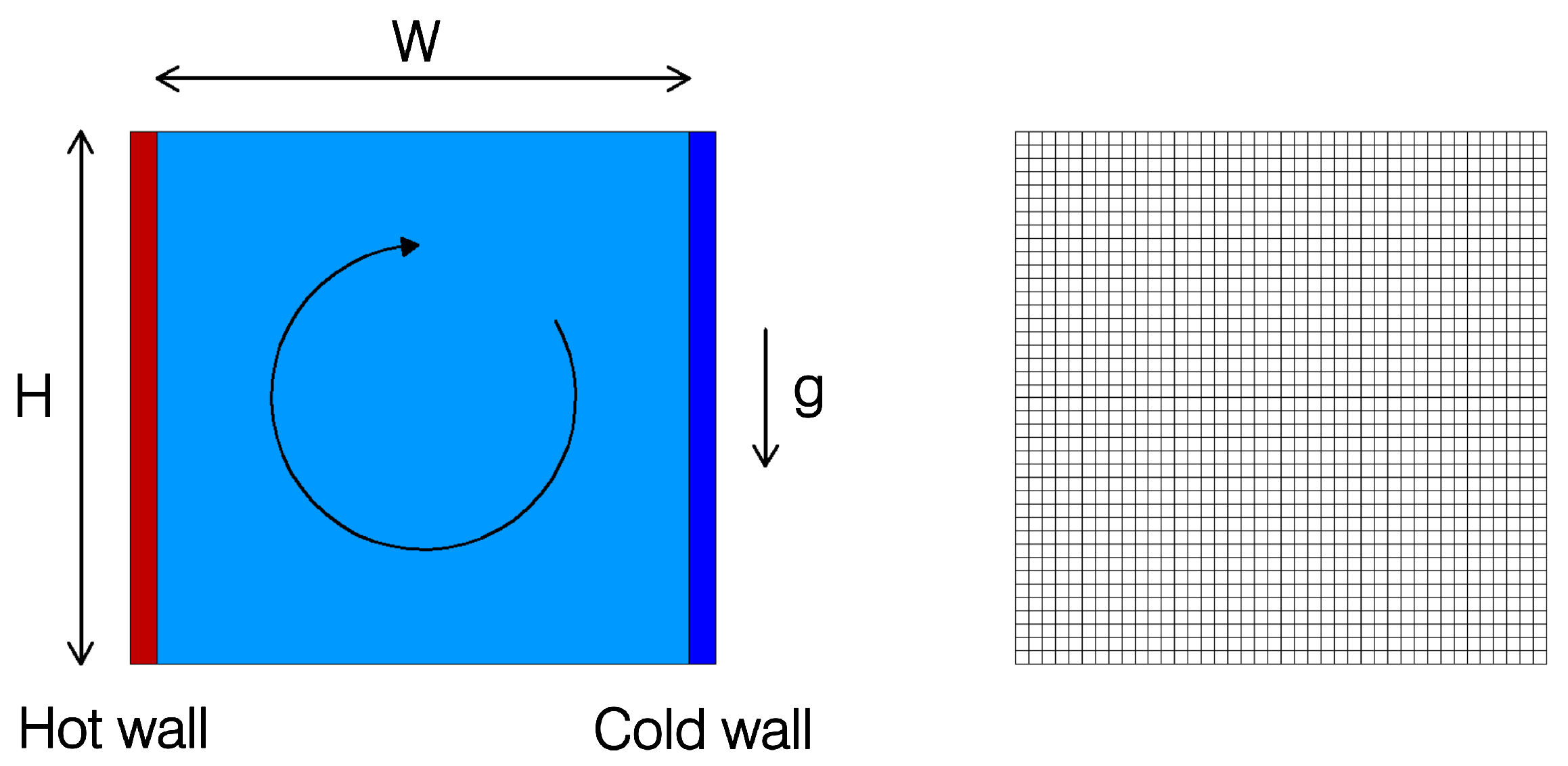
The implementation of molten-salt properties in CUPID-MSR was verified using the two-dimensional thermal cavity benchmark problem originally introduced by de Vahl Davis [18]. Figure 2 illustrates the schematic of the cavity configuration together with the computational mesh used in the simulations. The square cavity ($H=W$) is oriented so that gravity acts perpendicular to the cavity surface. Constant temperature boundary conditions are applied at the left and right walls, with the left wall maintained at a higher temperature than the right wall. The horizontal boundaries at the top and bottom are treated as adiabatic. Under these conditions, buoyancy-driven natural convection is expected to develop within the cavity.

In the present thermal cavity problem, the development of natural circulation is characterized by the Rayleigh number ($Ra$), defined as

$$Ra={\displaystyle \frac{{\rho }^{2}g\beta (T_{\mathrm{hot}}-T_{\mathrm{cold}})H^3}{{\mu }^2}}Pr,$$

(12)

where $\rho$, $\beta$, and g represent the fluid density, thermal expansion coefficient, and gravitational acceleration, respectively. The Prandtl number ($Pr$) is defined as $Pr=\left(C_p\mu \right)/\lambda$, where $C_p$ denotes the specific heat capacity and $\lambda$ the thermal conductivity. As the Rayleigh number increases, the flow gradually transitions from laminar toward turbulent conditions. The Rayleigh number was varied by adjusting the cavity height H, while the temperature difference $\Delta T=1\mathrm{K}$, gravitational acceleration, and thermophysical properties were kept constant.

The original de Vahl Davis benchmark corresponds to air with a Prandtl number of $Pr=0.71$, whereas the molten salts considered in the present study exhibit higher Prandtl numbers. At the reference temperature of $900\mathrm{K}$, the Prandtl numbers of KCl–UCl₃ and NaCl–MgCl₂–TRUCl₃ are approximately 5.1 and 3.9, respectively. To assess the influence of this difference on the benchmark comparison, additional calculations with an enforced $Pr=0.71$ were performed. The quantitative comparison is presented in Section 3.5.

The calculations were performed for ${10}^3\le Ra\le {10}^6$, corresponding to laminar flow conditions in the cavity. The temperatures of the hot and cold walls were set to 900.5 K and 899.5 K, respectively, corresponding to typical operating temperatures of proposed MSR designs.

3.2. Nusselt Number Evaluation Method

In this benchmark, the Nusselt number ($Nu$) is used as the primary metric for evaluating the verification results. The Nusselt number is a dimensionless quantity that characterizes the intensity of convective heat transfer relative to pure conduction. A value of $Nu=1$ corresponds to purely conductive heat transfer, while values greater than unity indicate enhancement due to convection. As the Rayleigh number increases, buoyancy forces intensify, leading to higher fluid velocities and an increased heat transfer coefficient, and consequently a larger Nusselt number.

In this work, heat transfer near the hot wall is characterized by the local Nusselt number, defined as

$$Nu=-{\displaystyle \frac{H}{\Delta T}}{\left({\displaystyle \frac{\partial T}{\partial x}}\right)}_{\mathrm{hot}},$$

(13)

where $\Delta T=T_{\mathrm{hot}}-T_{\mathrm{cold}}$. When a nondimensional temperature formulation is employed, the Nusselt number can be expressed as

$$Nu={\left({\displaystyle \frac{\partial T^{*}}{\partial x^{*}}}\right)}_{\mathrm{hot}},$$

(14)

with the non-dimensional variables defined as

$$T^{*}={\displaystyle \frac{T-T_{\mathrm{cold}}}{T_{\mathrm{hot}}-T_{\mathrm{cold}}}},x^{*}={\displaystyle \frac{x}{H}}.$$

(15)

The average Nusselt number along the hot wall is obtained by integrating the local Nusselt number over the vertical direction:

$$\overline{Nu}={\displaystyle \frac{1}{H}}{\int }_0^{H}Nudy.$$

(16)

For numerical evaluation, this integral is approximated using Simpson’s rule:

$$\overline{Nu}={\displaystyle \frac{1}{6}}\left[Nu\left(0\right)+4Nu\left({\displaystyle \frac{H}{2}}\right)+Nu\left(H\right)\right].$$

(17)

Accordingly, the local Nusselt number is evaluated at three vertical locations along the hot wall: the bottom, mid-height, and top of the cavity.

3.3. Mesh Sensitivity and Solution Verification

A mesh sensitivity study was performed to assess the influence of spatial discretization on the numerical solution and to ensure that the predicted heat transfer results are independent of grid resolution. In numerical simulations, insufficient mesh resolution may lead to discretization errors, particularly in regions with strong velocity and temperature gradients such as the thermal boundary layers near the cavity walls. Since the average Nusselt number is used as the primary verification metric in the de Vahl Davis benchmark, it is essential to confirm that this quantity converges with mesh refinement. Therefore, a grid convergence analysis was conducted to evaluate the sensitivity of the predicted Nusselt number to mesh resolution and to estimate the associated discretization uncertainty. The verification methodology applied in this work follows the general framework for grid convergence assessment described by Roache [32], which employs systematic mesh refinement together with Richardson extrapolation and the Grid Convergence Index (GCI) to quantify discretization errors.

3.3.1. Apparent Order of Spatial Accuracy

To quantify the spatial discretization error of the primary verification metric, a formal grid convergence analysis was performed using the average Nusselt number. Three systematically refined meshes consisting of $30\times 30$, $60\times 60$, and $120\times 120$ control volumes were selected for this assessment, corresponding to a constant refinement ratio of $r=2$. Stronger thermal and velocity gradients develop near the cavity walls at the highest Rayleigh number ($Ra={10}^6$), resulting in thinner boundary layers that require increased spatial resolution. To better capture these gradients, an additional refinement level was introduced, and the mesh triplet ($40\times 40$, $80\times 80$, $160\times 160$) was employed while preserving the same refinement ratio. The corresponding average Nusselt numbers obtained on the grid sequences are summarized in

Table 2. Average Nusselt numbers obtained for the standard three-grid sequence ($30\times 30$, $60\times 60$, $120\times 120$) used in the spatial convergence analysis for $Ra={10}^3$–${10}^5$.

Ra	KCl–UCl3			NaCl–MgCl2–TRUCl3
	$\mathbf{30}\times \mathbf{30}$	$\mathbf{60}\times \mathbf{60}$	$\mathbf{120}\times \mathbf{120}$	$\mathbf{30}\times \mathbf{30}$	$\mathbf{60}\times \mathbf{60}$	$\mathbf{120}\times \mathbf{120}$
${10}^3$	1.1297	1.1221	1.1190	1.1170	1.1107	1.1078
${10}^4$	2.2041	2.1815	2.1749	2.2482	2.2315	2.2271
${10}^5$	4.8140	4.6180	4.5638	4.7287	4.5599	4.5118

and

Table 3. Average Nusselt numbers obtained for the refined three-grid sequence ($40\times 40$, $80\times 80$, $160\times 160$) used in the spatial convergence analysis for $Ra={10}^6$.

Ra	KCl–UCl3			NaCl–MgCl2–TRUCl3
	$\mathbf{40}\times \mathbf{40}$	$\mathbf{80}\times \mathbf{80}$	$\mathbf{160}\times \mathbf{160}$	$\mathbf{40}\times \mathbf{40}$	$\mathbf{80}\times \mathbf{80}$	$\mathbf{160}\times \mathbf{160}$
${10}^6$	9.7699	9.1401	8.8691	9.5523	8.9568	8.6965

.

Following the verification procedure described by Roache [32], the apparent order of spatial accuracy was estimated from the variation in the average Nusselt number obtained on the three meshes. The apparent order p was calculated using the standard three-grid formulation:

$$p={\displaystyle \frac{ln\left|\frac{{\overline{Nu}}_{\mathrm{coarse}}-{\overline{Nu}}_{\mathrm{medium}}}{{\overline{Nu}}_{\mathrm{medium}}-{\overline{Nu}}_{\mathrm{fine}}}\right|}{ln\left(r\right)}}.$$

(18)

where ${\overline{Nu}}_{\mathrm{coarse}}$, ${\overline{Nu}}_{\mathrm{medium}}$, and ${\overline{Nu}}_{\mathrm{fine}}$ denote the average Nusselt numbers obtained on the coarse, medium, and fine meshes of the grid sequence, respectively. The refinement ratio r is defined as the ratio of the characteristic grid spacings between two consecutive meshes and is equal to $r=2$ for all grid sequences considered in this study. The calculated apparent orders of spatial accuracy obtained from the mesh triplets are summarized in

Table 4. Grid convergence analysis for the average Nusselt number based on the mesh triplet ($30\times 30$, $60\times 60$, $120\times 120$) for $Ra\le {10}^5$ and ($40\times 40$, $80\times 80$, $160\times 160$) for $Ra={10}^6$. The table lists the apparent order of spatial accuracy p, the Richardson-extrapolated Nusselt number $N{u}_{\mathrm{ext}}$, the fine-grid discretization error, and the GCI.

Ra	KCl–UCl3				NaCl–MgCl2–TRUCl3
	$\mathit{p}$	${\mathit{Nu}}_{\mathbf{ext}}$	${\mathit{\epsilon }}_{\mathbf{ext}}$ (%)	GCIfine (%)	$\mathit{p}$	${\mathit{Nu}}_{\mathbf{ext}}$	${\mathit{\epsilon }}_{\mathbf{ext}}$ (%)	GCIfine (%)
${10}^3$	1.29	1.1169	0.19	0.24	1.12	1.1053	0.22	0.28
${10}^4$	1.78	2.1722	0.13	0.16	1.93	2.2255	0.07	0.09
${10}^5$	1.85	4.5430	0.46	0.57	1.81	4.4926	0.43	0.53
${10}^6$	1.22	8.6645	2.36	2.88	1.19	8.4944	2.38	2.91

together with the Richardson-extrapolated Nusselt numbers and the associated discretization error estimates used in the grid convergence analysis.

The results show that the observed order of accuracy varies with the Rayleigh number. For the lowest Rayleigh number ($Ra={10}^3$), the apparent order of spatial accuracy is relatively low ($p\approx 1.1$–$1.3$), which can be attributed to the weak convective motion and the dominance of diffusive heat transfer in the cavity. As the Rayleigh number increases to $Ra={10}^4$ and $Ra={10}^5$, the observed order increases and approaches second-order accuracy ($p\approx 1.8$–$1.9$), which is consistent with the second-order spatial discretization employed in the numerical scheme.

For the highest Rayleigh number ($Ra={10}^6$), an additional grid refinement level was introduced and the mesh triplet ($40\times 40$, $80\times 80$, $160\times 160$) was used in the convergence analysis. With this refined grid sequence, the observed order of accuracy increases to approximately $p\approx 1.2$, indicating improved spatial convergence compared to the coarser mesh sequence. The remaining deviation from second-order accuracy can be attributed to the formation of increasingly thin thermal boundary layers and strong velocity gradients near the cavity walls, which are characteristic of high-Rayleigh-number natural convection and require very fine grid resolution for full asymptotic behavior.

Nevertheless, the Nusselt number decreases monotonically with grid refinement for all cases, indicating consistent spatial convergence toward a mesh-independent solution.

3.3.2. Richardson Extrapolation of the Average Nusselt Number

To further quantify the discretization error associated with the mesh resolution, Richardson extrapolation was applied to the computed average Nusselt numbers. The analysis was performed using three systematically refined meshes with a constant refinement ratio $r=2$. For $Ra\le {10}^5$ the grid triplet ($30\times 30$, $60\times 60$, $120\times 120$) was used, while for $Ra={10}^6$ the refined triplet ($40\times 40$, $80\times 80$, $160\times 160$) was applied.

Using the apparent order of spatial accuracy p obtained from the three-grid sequence, the Richardson-extrapolated Nusselt number was calculated according to

$${\overline{Nu}}_{\mathrm{ext}}={\overline{Nu}}_{\mathrm{fine}}+{\displaystyle \frac{{\overline{Nu}}_{\mathrm{fine}}-{\overline{Nu}}_{\mathrm{medium}}}{r^p-1}}.$$

(19)

where ${\overline{Nu}}_{\mathrm{fine}}$ and ${\overline{Nu}}_{\mathrm{medium}}$ denote the average Nusselt numbers obtained on the fine and medium meshes of the grid sequence, respectively. The extrapolated value represents an estimate of the asymptotic solution corresponding to zero grid spacing.

The remaining discretization error associated with the fine-grid solution was estimated by evaluating the relative difference between the Richardson-extrapolated value and the computed result on the finest mesh:

$${\epsilon }_{\mathrm{ext}}=\left|{\displaystyle \frac{{\overline{Nu}}_{\mathrm{ext}}-{\overline{Nu}}_{\mathrm{fine}}}{{\overline{Nu}}_{\mathrm{ext}}}}\right|\times 100.$$

(20)

The extrapolated Nusselt numbers and the corresponding discretization error estimates are summarized in Table 4 together with the apparent order of spatial accuracy obtained from the mesh triplets. These quantities provide a quantitative assessment of grid convergence and serve as the basis for the subsequent GCI analysis used to estimate the discretization uncertainty.

3.3.3. Grid Convergence Index (GCI)

The Grid Convergence Index (GCI) provides a standardized measure of the numerical uncertainty associated with spatial discretization by estimating the distance between the computed solution and the asymptotic grid-independent solution.

To quantify this uncertainty, the GCI was evaluated using the three-grid sequences employed in the grid convergence analysis. For $Ra\le {10}^5$ the mesh triplet ($30\times 30$, $60\times 60$, $120\times 120$) was used, while for $Ra={10}^6$ the refined sequence ($40\times 40$, $80\times 80$, $160\times 160$) was applied.

First, the relative difference between the medium and fine grid solutions was computed as

$$\epsilon ={\displaystyle \frac{{\overline{Nu}}_{\mathrm{medium}}-{\overline{Nu}}_{\mathrm{fine}}}{{\overline{Nu}}_{\mathrm{fine}}}}.$$

(21)

where ${\overline{Nu}}_{\mathrm{medium}}$ and ${\overline{Nu}}_{\mathrm{fine}}$ denote the average Nusselt numbers obtained on the medium and fine meshes of the grid sequence, respectively. This quantity represents the relative difference between the two finest grid solutions.

The GCI for the fine-grid solution was then calculated as

$${\mathrm{GCI}}_{\mathrm{fine}}=F_s{\displaystyle \frac{\left|\epsilon \right|}{r^p-1}},$$

(22)

where r is the grid refinement ratio and p is the apparent order of spatial accuracy obtained from the grid triplet. For all mesh sequences considered in this study the refinement ratio is $r=2$. A safety factor of $F_s=1.25$ was adopted, consistent with the recommendation for three-grid convergence studies in which the observed order of accuracy is determined from the grid sequence.

The resulting GCI values for the fine grid are summarized in Table 4. For Rayleigh numbers up to $Ra={10}^5$, the estimated discretization uncertainty remains below approximately $0.6\%$ for both salt mixtures, indicating that the selected mesh resolution is sufficiently close to the asymptotic solution for these cases.

At the highest Rayleigh number considered ($Ra={10}^6$), the additional refinement level reduces the estimated discretization uncertainty to approximately $3\%$ for both salt mixtures. Although the observed order of spatial accuracy remains below the nominal second-order accuracy of the numerical scheme, the results still exhibit monotonic convergence and remain within a reasonable uncertainty range. The remaining discretization error can be attributed to the increasingly thin thermal boundary layers and strong velocity and temperature gradients that develop at high Rayleigh numbers, which require very fine grid resolution for full asymptotic behavior.

3.3.4. Grid Convergence Behaviour

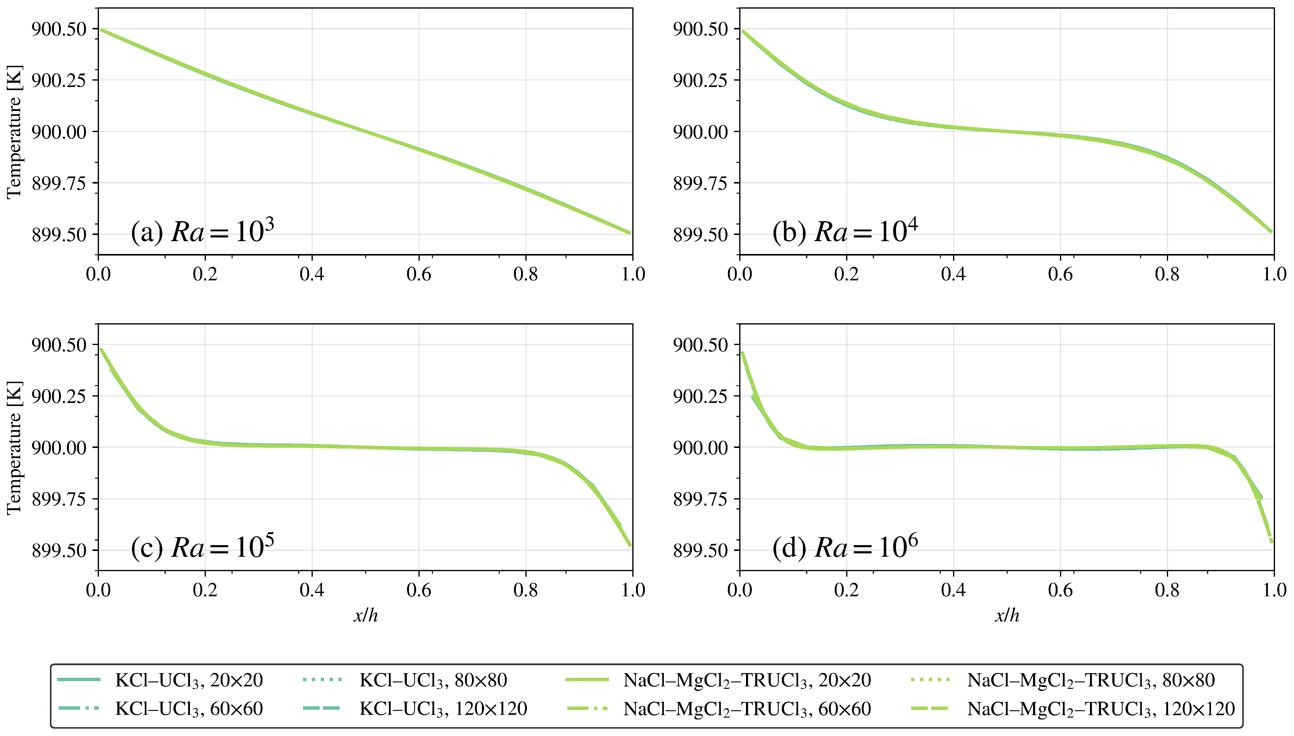
As an additional qualitative illustration of the grid convergence behaviour, Figure 3 presents the column-averaged temperature profile $\overline{T}(x/H)$ across the cavity, obtained by averaging the temperature along the vertical direction at each non-dimensional horizontal position $x/H$. This global metric reflects the overall thermal distribution within the cavity and provides a convenient visualization of the convergence behaviour without focusing on localized flow quantities. For clarity, results obtained using four meshes ($20\times 20$, $60\times 60$, $80\times 80$, and $120\times 120$) are shown.

Across all Rayleigh numbers and for both salt mixtures, temperature profiles obtained on the finer meshes ($60\times 60$, $80\times 80$, and $120\times 120$) collapse onto a single curve, indicating that the global temperature distribution becomes essentially mesh-independent once a moderately fine grid is used. The coarsest mesh ($20\times 20$) exhibits minor deviations, which become noticeable primarily at the highest Rayleigh numbers.

Both molten-salt mixtures exhibit nearly identical convergence behaviour, with only negligible differences in the column-averaged temperature profiles across the investigated Rayleigh number range. These observations provide additional qualitative evidence that the selected mesh resolutions are sufficient to capture the dominant thermal transport mechanisms within the cavity before examining more sensitive near-wall quantities.

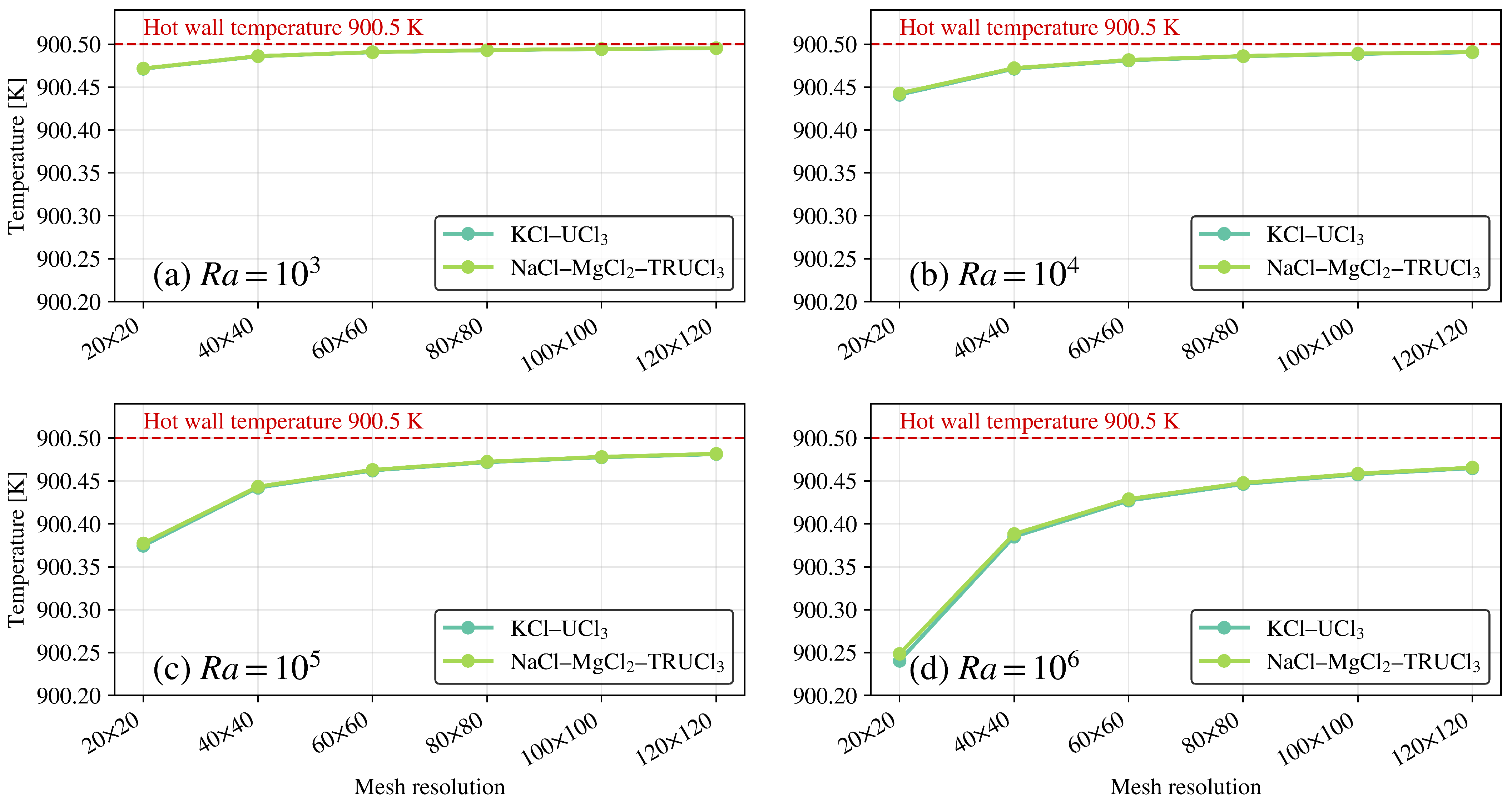
A more sensitive indicator of mesh dependence is the temperature in the first column of cells adjacent to the hot wall, shown in Figure 4. Because this region contains the steepest thermal gradients, it is particularly sensitive to grid resolution and therefore useful for assessing the mesh density required to resolve the thermal boundary layer. As the mesh is refined, the near-wall temperature monotonically approaches the imposed hot-wall temperature of 900.5 K, demonstrating consistent convergence behaviour.

These qualitative observations are consistent with the quantitative convergence analysis presented earlier based on Richardson extrapolation and the GCI, and further support the mesh resolutions selected for the simulations.

3.3.5. Summary of Mesh Sensitivity Analysis

Based on the mesh sensitivity analysis, different mesh resolutions were selected for the final simulations depending on the Rayleigh number, as summarized in

Table 5. Selected mesh resolutions and corresponding cavity heights used in the simulations.

Rayleigh Number ($\mathit{Ra}$)	${10}^3$	${10}^4$	${10}^5$	${10}^6$
Mesh resolution	$40\times 40$	$60\times 60$	$60\times 60$	$80\times 80$
KCl–UCl3	0.003504	0.007549	0.016265	0.035041
NaCl–MgCl2–TRUCl3	0.004151	0.008943	0.019267	0.041510

. As the Rayleigh number increases, buoyancy-driven convection intensifies and progressively thinner thermal boundary layers develop near the hot and cold walls, which require finer spatial resolution to be accurately captured.

The mesh sensitivity results indicate that for the lowest Rayleigh number ($Ra={10}^3$) the predicted Nusselt number becomes essentially mesh-independent already on a $40\times 40$ grid. For $Ra={10}^4$ and $Ra={10}^5$, stronger convective circulation leads to steeper temperature gradients near the walls, and a $60\times 60$ mesh provides sufficient resolution of the thermal boundary layers while maintaining reasonable computational cost.

For the highest Rayleigh number ($Ra={10}^6$), the flow develops significantly thinner thermal boundary layers and stronger velocity gradients. To better assess the spatial discretization uncertainty for this case, an additional grid refinement level ($160\times 160$) was introduced in the convergence analysis. The resulting GCI analysis indicates that the estimated discretization uncertainty decreases to approximately $3\%$ for both salt mixtures, confirming that the solution exhibits monotonic convergence with grid refinement. Although this case remains more sensitive to mesh resolution than the lower Rayleigh numbers, the $80\times 80$ grid provides a reasonable compromise between numerical accuracy and computational efficiency.

Further refinement beyond the selected meshes produces only modest changes in the predicted average Nusselt number, indicating that the numerical solution is approaching grid-independent behavior within the estimated discretization uncertainty for the investigated Rayleigh numbers.

3.4. Comparison with Benchmark Solution

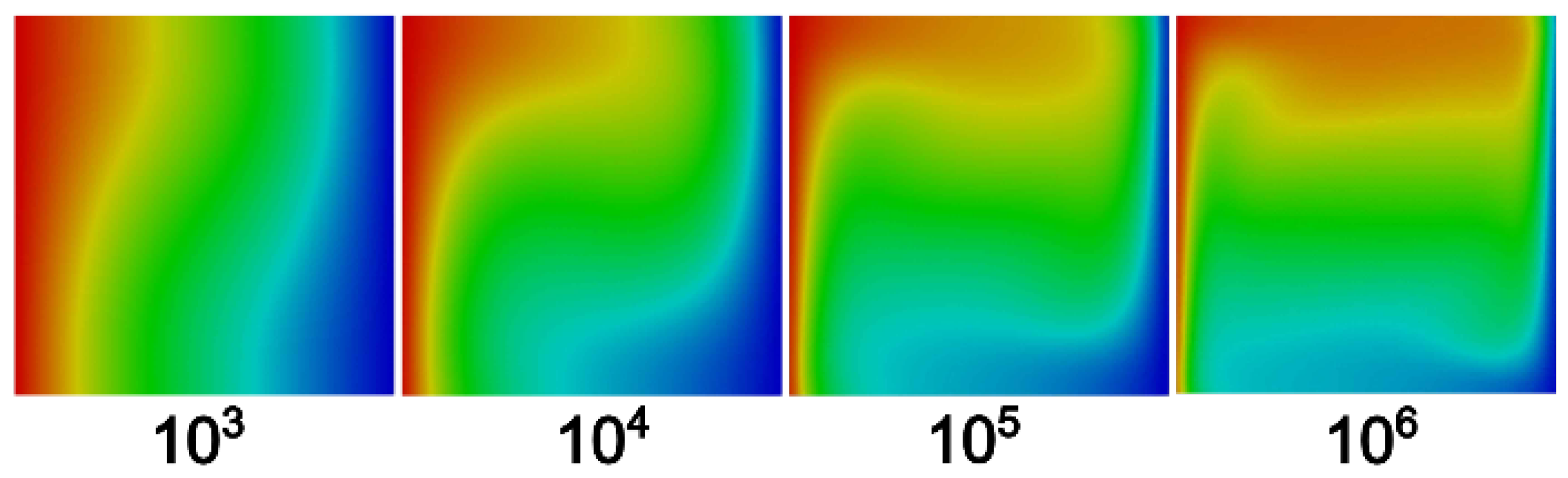
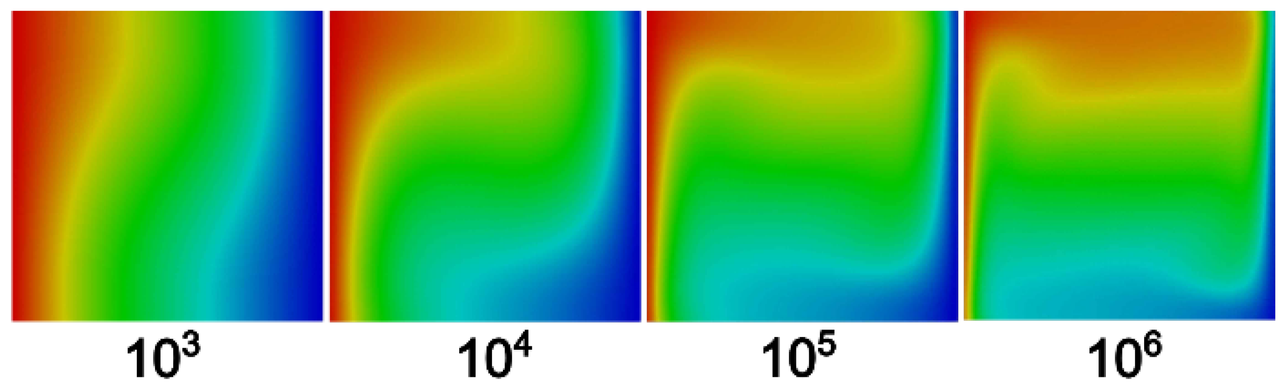
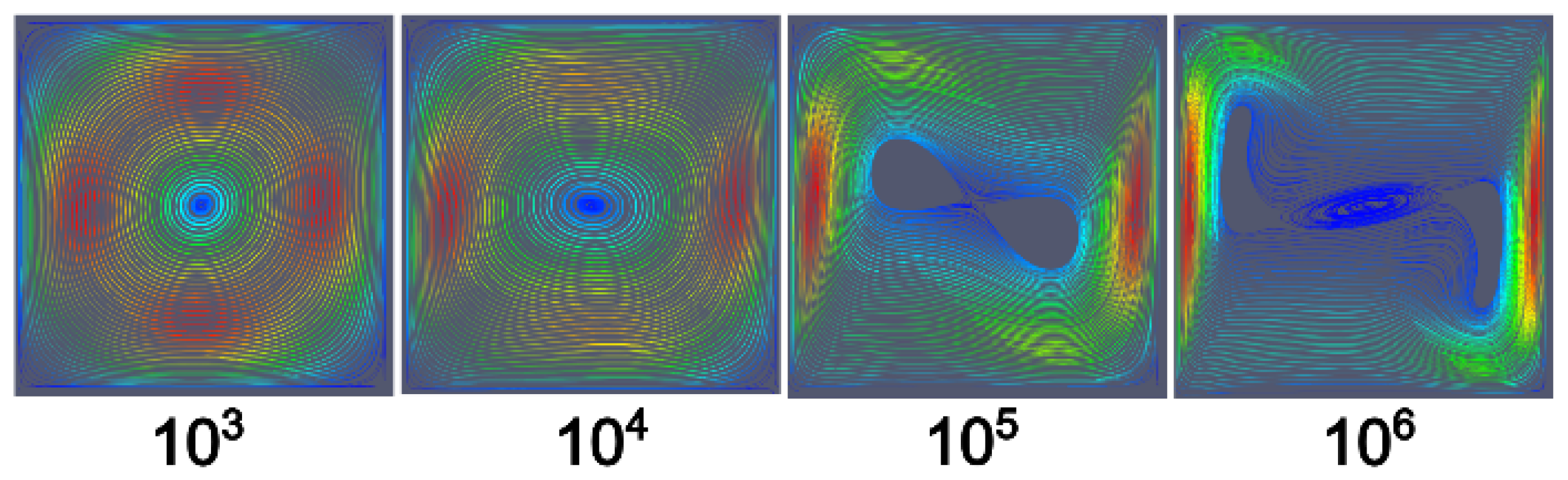
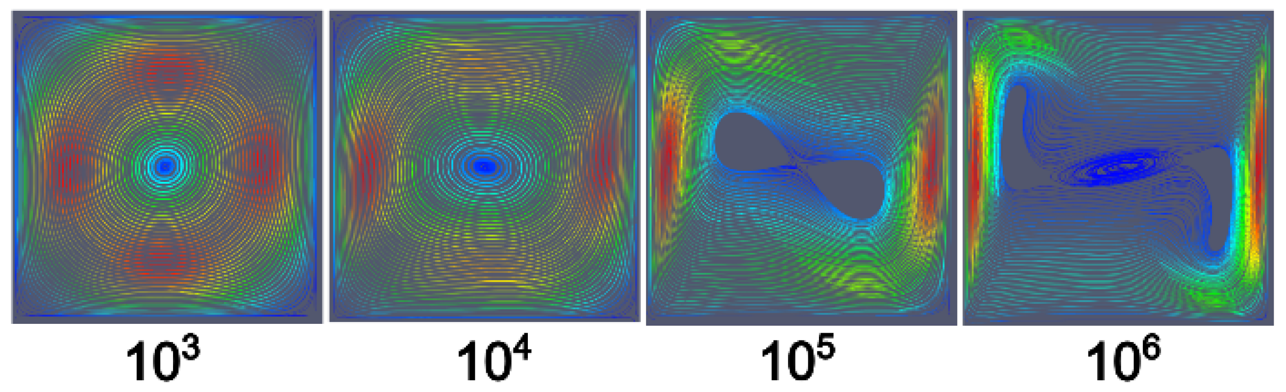
Figure 5 and Figure 6 illustrate the temperature contour fields for KCl–UCl₃ and NaCl–MgCl₂–TRUCl₃ at various Rayleigh numbers. The corresponding streamline patterns are shown in Figure 7 and Figure 8. In all cases, buoyancy-driven natural convection develops clockwise within the cavity. As the Rayleigh number increases, buoyancy-driven circulation becomes stronger, resulting in thinner thermal boundary layers and the formation of additional corner vortices. At $Ra={10}^3$ and $Ra={10}^4$, the flow is dominated by a single recirculating cell; at $Ra={10}^5$, two vortices are observed; and at $Ra={10}^6$, three distinct vortical structures emerge. The decreasing boundary-layer thickness with increasing $Ra$ indicates stronger heat transfer at both the hot and cold walls.

A qualitative comparison of the temperature contours (Figure 5 and Figure 6) and streamline patterns (Figure 7 and Figure 8) with the reference de Vahl Davis benchmark confirms that CUPID-MSR successfully reproduces the characteristic temperature distributions and flow-field structures. The close agreement in vortex formation and isotherm topology provides qualitative support for the implemented buoyancy and thermophysical property models, and indicates the correct computation of the Rayleigh number in the code.

Quantitatively, the average Nusselt numbers predicted by CUPID-MSR are compared with benchmark data in

Table 6. Comparison of average Nusselt numbers predicted by CUPID-MSR with the de Vahl Davis benchmark.

Calculation	${10}^3$	${10}^4$	${10}^5$	${10}^6$
de Vahl Davis	1.118	2.243	4.519	8.800
CUPID-MSR (KCl–UCl3)	1.1253 (0.66) *	2.1815 (2.74) *	4.6180 (2.19) *	9.1401 (3.86) *
CUPID-MSR (NaCl–MgCl2–TRUCl3)	1.1137 (0.38) *	2.2315 (0.51) *	4.5599 (0.91) *	8.9568 (1.78) *

* Percentage deviation from the de Vahl Davis benchmark solution.

for both molten-salt mixtures. The relative deviation of the average Nusselt number is defined as the percentage difference between the computed value and the benchmark reference at the same Rayleigh and Prandtl numbers:

$${\epsilon }_{Nu}={\displaystyle \frac{\left|{\overline{Nu}}_{\mathrm{CUPID-MSR}}-{\overline{Nu}}_{\mathrm{DVD}}\right|}{{\overline{Nu}}_{\mathrm{DVD}}}}\times 100\%.$$

(23)

The deviations from the reference solution range from 0.66% to 3.86% for KCl–UCl₃ and from 0.38% to 1.78% for NaCl–MgCl₂–TRUCl₃. A direct comparison between the two salt mixtures shows that both follow the same heat transfer trend, with only minor differences in the predicted Nusselt numbers. The maximum difference between the two solutions remains within 1.04% for $Ra\le {10}^3$, 2.24% for $Ra\le {10}^4$, 1.27% for $Ra\le {10}^5$, and 2.04% for $Ra\le {10}^6$.

In both molten-salt cases, the predicted Nusselt numbers increase monotonically with Rayleigh number, consistent with the benchmark trend and reflecting progressively stronger convective heat transport. The discrepancy between the numerical predictions and the reference solution increases slightly with Rayleigh number as the flow develops thinner boundary layers and stronger gradients.

3.5. Influence of the Prandtl Number

As noted in Section 3.1, the original de Vahl Davis benchmark corresponds to air with a Prandtl number of $Pr=0.71$, whereas the molten salts considered in the present work exhibit higher Prandtl numbers. At the reference temperature of $900\mathrm{K}$, the Prandtl numbers of KCl–UCl₃ and NaCl–MgCl₂–TRUCl₃ are approximately $Pr\approx 5.1$ and $Pr\approx 3.9$, respectively. To evaluate the influence of this difference on the benchmark comparison, additional calculations were performed in which the Prandtl number was artificially enforced to $Pr=0.71$.

To achieve this, the thermal conductivity in the property correlations was adjusted such that the Prandtl number remained constant at $Pr=0.71$ while keeping the remaining thermophysical properties unchanged. This modification allows a direct comparison with the original de Vahl Davis benchmark conditions while isolating the effect of the Prandtl number on the predicted heat transfer.

Table 7. Comparison of average Nusselt numbers obtained using the physical molten-salt Prandtl number and an artificially enforced $Pr=0.71$ for the KCl–UCl₃ mixture at $900\mathrm{K}$.

Calculation	${10}^3$	${10}^4$	${10}^5$	${10}^6$
$\overline{Nu}$ (physical $Pr\approx 5.1$)	1.1253	2.1815	4.6180	9.1401
$\overline{Nu}$ (enforced $Pr=0.71$)	1.1242	2.1774	4.6000	9.0935
Difference (%)	0.10	0.19	0.39	0.51

presents the quantitative comparison of the average Nusselt numbers obtained using the physically consistent molten-salt properties and those obtained using the enforced $Pr=0.71$ for the KCl–UCl₃ mixture at $900\mathrm{K}$. The calculations were performed for Rayleigh numbers ranging from ${10}^3$ to ${10}^6$.

The results show that enforcing the benchmark Prandtl number produces only minor changes in the predicted Nusselt number across the investigated Rayleigh number range. As shown in Table 7, the relative difference between the two cases increases slightly with Rayleigh number but remains below $0.6\%$ for all investigated conditions.

Because enforcing a constant $Pr=0.71$ requires modifying the thermal conductivity and therefore deviates from the physical thermophysical properties of molten salts, the verification results presented in this work are based on the physically consistent temperature-dependent property correlations. Nevertheless, the comparison demonstrates that the difference in Prandtl number has a negligible influence on the predicted Nusselt numbers in the investigated regime, confirming that the benchmark comparison remains valid despite the higher Prandtl numbers of the molten salts.

3.6. Temperature Variation Sensitivity

To further assess the temperature dependence of the implemented thermophysical property correlations, an additional sensitivity analysis was performed by varying the reference temperature of the thermal cavity. The objective of this study was to quantify how changes in the molten-salt fluid temperature influence the accuracy of the predicted average Nusselt number in CUPID-MSR relative to the benchmark solution.

Simulations were carried out for both molten-salt mixtures over a range of Rayleigh numbers, with fluid temperatures spanning from 800 K to 2000 K and appropriately selected temperature increments, while maintaining the same boundary-condition configuration as in the reference case. Because molten-salt properties such as density, viscosity, thermal conductivity, and heat capacity exhibit strong temperature dependence, even modest temperature variations can significantly alter the resulting Rayleigh and Prandtl numbers and, consequently, the heat transfer behavior.

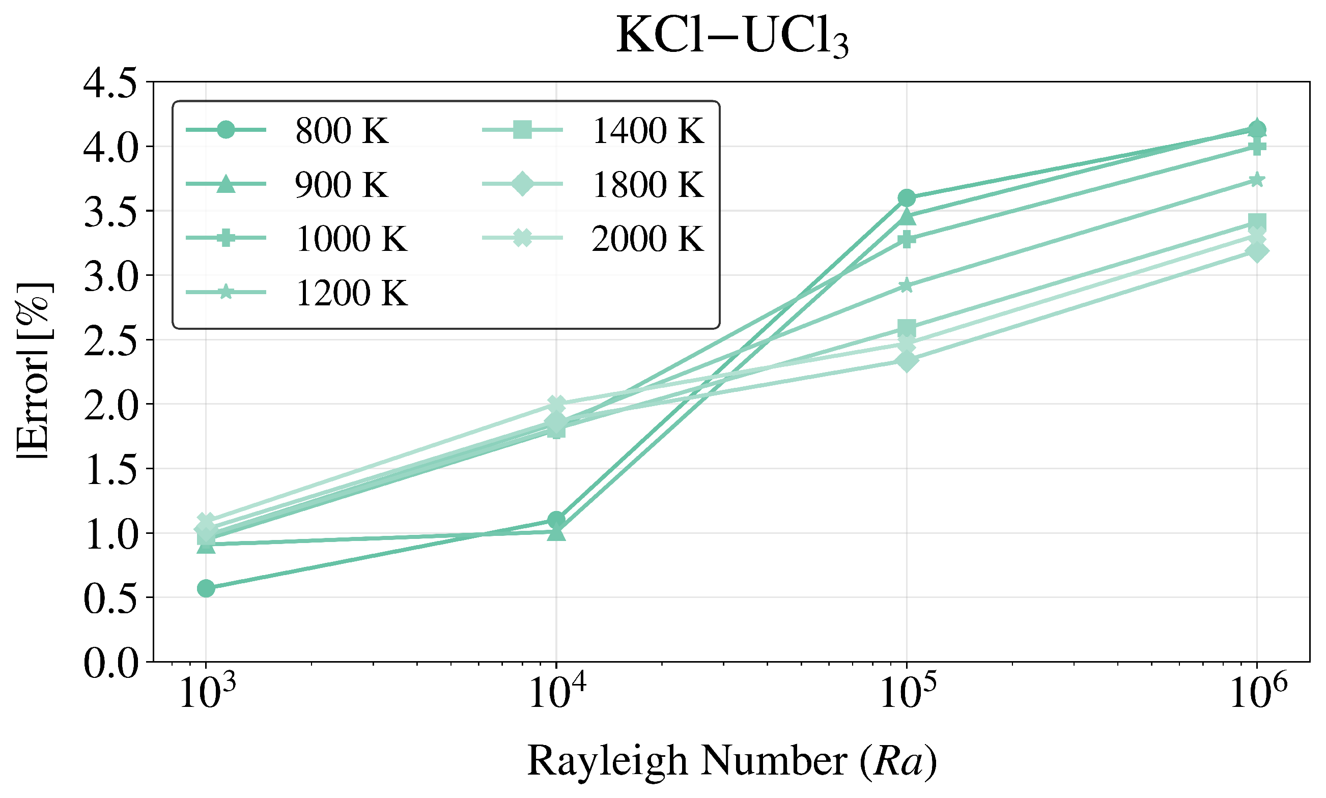
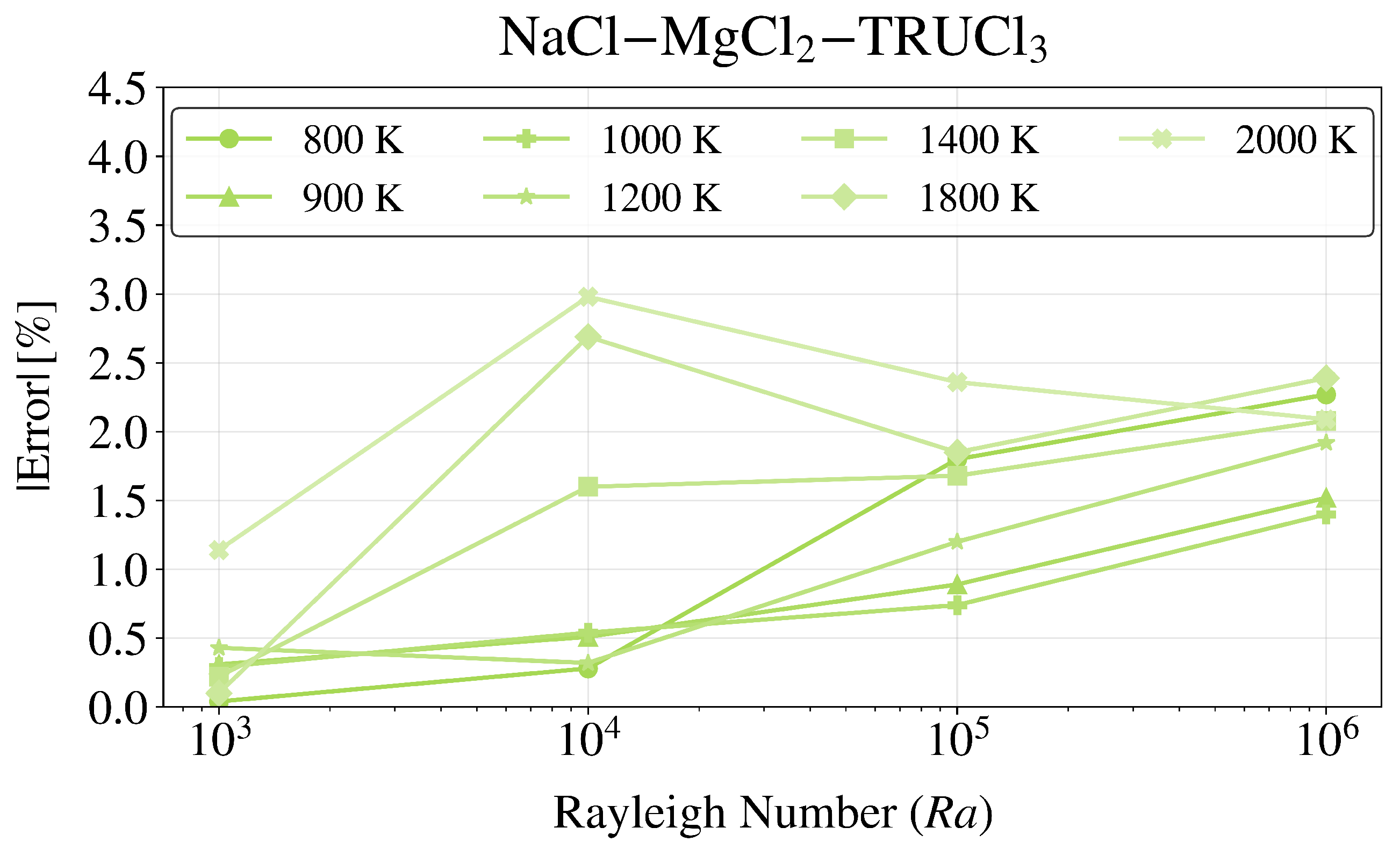
Figure 9 and Figure 10 present the relative deviations of the average Nusselt numbers from the de Vahl Davis benchmark for the KCl–UCl₃ and NaCl–MgCl₂–TRUCl₃ mixtures, respectively. For KCl–UCl₃, the deviation remains below 4.3%, while for NaCl–MgCl₂–TRUCl₃ it consistently remains below 3.0%. These results confirm that the implemented property correlations provide stable and reliable predictions over a wide temperature range.

The results also indicate that the deviation in the Nusselt number generally increases with increasing Rayleigh number. This behavior can be attributed to stronger buoyancy-driven convection at higher $Ra$ values. At low Rayleigh numbers, heat transfer is dominated by conduction and the velocity field is weak, resulting in smooth temperature gradients and close agreement with the benchmark solution. As $Ra$ increases, buoyancy forces intensify and more pronounced circulation develops, producing steeper velocity and temperature gradients near the hot and cold walls. These gradients are more challenging to resolve numerically, leading to slightly larger deviations from the reference data.

Overall, this sensitivity analysis demonstrates that both molten-salt mixtures maintain good agreement with the benchmark solution across the investigated temperature range, indicating that CUPID-MSR can reliably simulate MSR conditions under typical operating temperatures as well as during transients involving moderate temperature increases.

4. Assessment of the Boussinesq Approximation

Natural convection in molten-salt systems is strongly influenced by temperature-dependent density variations. In many CFD and system codes, buoyancy-driven flow is modeled using the Boussinesq approximation. Under this assumption, density is treated as constant in all terms of the momentum equation except for the buoyancy term, where its linear dependence on temperature is preserved. Although this approximation is widely applied to water and air flows, its applicability to molten salts—characterized by high density, strong thermophysical gradients, and potentially nonlinear $\rho \left(T\right)$ behavior—has not been systematically assessed.

The applicability of the Boussinesq approximation has been widely discussed in the natural-convection literature. A commonly cited guideline states that the approximation remains accurate when density variations are small, typically when the relative density change $\beta \Delta T$ does not exceed approximately 0.1 [33,34].

Because CUPID-MSR relies on temperature-dependent molten-salt properties to accurately model buoyancy-driven flow, it is important to determine the temperature range over which the Boussinesq approximation remains valid for chloride-based MSR fluids. Therefore, this section evaluates the accuracy of the Boussinesq approximation by comparing it with the full variable-density formulation of CUPID-MSR using the de Vahl Davis natural-convection benchmark. Although molten-salt thermophysical properties are employed, the applicability of the Boussinesq approximation is governed by the nondimensional parameter $\beta \Delta T$, which represents the relative density variation and is therefore independent of the specific working fluid. Consequently, the results obtained here are relevant not only for molten salts but also for a broad class of buoyancy-driven flows.

4.1. Full Variable-Density and Boussinesq Models

The Boussinesq approximation assumes that the fluid density remains constant throughout the computational domain, except in the buoyancy term of the momentum conservation equation, where a linear dependence on temperature is retained. This simplification reduces the computational cost of solving the Navier–Stokes equations while still capturing the dominant driving mechanism of natural convection.

In the full momentum conservation equation, density is treated as a temperature-dependent variable and appears in all inertial and gravitational terms. The governing equation can be expressed as

$$\rho \left(T\right)\left({\displaystyle \frac{\partial \overrightarrow{u}}{\partial t}}+\overrightarrow{u}·\nabla \overrightarrow{u}\right)=-\nabla p+\mu {\nabla }^2\overrightarrow{u}+\rho \left(T\right)\overrightarrow{g},$$

(24)

where $\rho \left(T\right)$ denotes the temperature-dependent fluid density.

When the Boussinesq approximation is applied, the momentum equation is written as

$${\rho }_{\mathrm{ref}}\left({\displaystyle \frac{\partial \overrightarrow{u}}{\partial t}}+\overrightarrow{u}·\nabla \overrightarrow{u}\right)=-\nabla p+\mu {\nabla }^2\overrightarrow{u}+{\rho }_{\mathrm{ref}}\beta (T-T_{\mathrm{ref}})\overrightarrow{g},$$

(25)

where T is the local fluid temperature, $T_{\mathrm{ref}}$ is the reference temperature, and ${\rho }_{\mathrm{ref}}$ is the density evaluated at $T_{\mathrm{ref}}$. The coefficient $\beta$ denotes the thermal expansion coefficient evaluated at the reference temperature.

These two formulations highlight the fundamental difference between the full variable-density model and the Boussinesq approximation. In the full formulation, $\rho \left(T\right)$ affects both inertial and buoyancy terms, whereas under the Boussinesq approximation, density is treated as constant in all terms except for the buoyancy force, where its linear temperature dependence is preserved. This approach retains the correct physical mechanism driving natural convection while significantly simplifying the governing equations.

4.2. Numerical Methodology

The applicability of the Boussinesq approximation was assessed using the same de Vahl Davis cavity configuration described in Section 3. All simulations in this study were performed for the KCl–UCl₃ salt mixture at a reference temperature of 900 K and at a fixed Rayleigh number of ${10}^3$. All geometric parameters, boundary conditions, and solver settings were kept identical to ensure that differences in the predicted Nusselt numbers originate solely from the treatment of density.

The temperature difference between the hot and cold walls was varied from 0.2 K to 400 K. For each case, the thermal expansion coefficient $\beta$ was obtained from the implemented density correlations, including the O1 linear reference model and two O3 nonlinear variants (O3–Variant A and O3–Variant B). For each density model, two types of simulations were conducted:

• The full variable-density formulation;
• The Boussinesq formulation, in which density is treated as constant in all momentum terms except for buoyancy.

The latter was implemented through a minor modification of the CUPID-MSR source code to ensure that density remained fixed in all non-buoyancy momentum contributions. Deviations from the benchmark were evaluated using the same relative error definition introduced in Section 3.4. Presenting the results as a function of the nondimensional parameter $\beta \Delta T$ enables a direct assessment of the temperature range over which the Boussinesq approximation remains accurate for molten-salt natural convection. Because $\beta \Delta T$ represents the relative density variation, the same methodology is applicable to any Newtonian fluid.

4.3. Linearization of Density

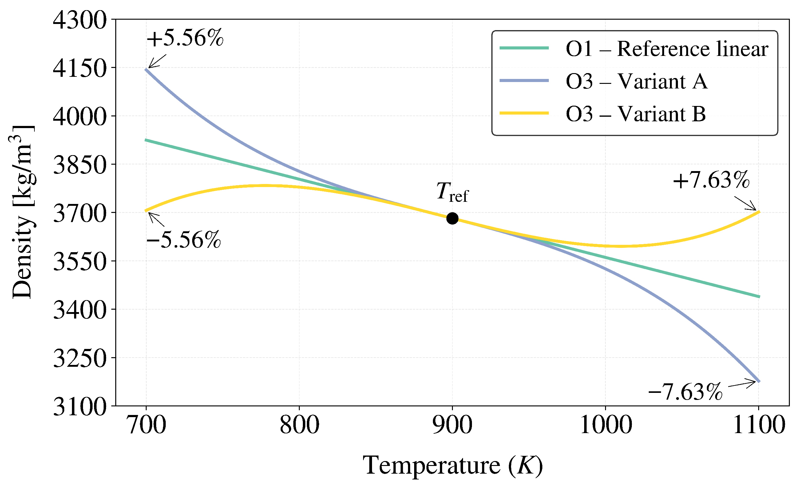
Figure 11 compares the three density–temperature correlations examined in this study. The O1 linear correlation corresponds to the original KCl–UCl₃ density model introduced in Equation (4). This linear model is equivalent to retaining only the first-order term of the Taylor expansion of the density field about the reference temperature $T_{\mathrm{ref}}=900\mathrm{K}$:

$$\rho \left(T\right)=\rho \left(T_{\mathrm{ref}}\right)+{\left.{\displaystyle \frac{\partial \rho }{\partial T}}\right|}_{T_{\mathrm{ref}}}(T-T_{\mathrm{ref}})+{\displaystyle \frac{1}{2}}{\left.{\displaystyle \frac{{\partial }^2\rho }{\partial T^2}}\right|}_{T_{\mathrm{ref}}}{(T-T_{\mathrm{ref}})}^2+\dots ,$$

(26)

Truncating this expansion after the linear term yields the familiar form

$$\rho \left(T\right)\approx {\rho }_{\mathrm{ref}}\left[1-\beta (T-T_{\mathrm{ref}})\right],$$

(27)

which is exactly the density model employed under the Boussinesq approximation. Here, the thermal expansion coefficient $\beta$ is defined at the reference temperature as $\beta =-{\displaystyle \frac{1}{{\rho }_{\mathrm{ref}}}}{\left.{\displaystyle \frac{\partial \rho }{\partial T}}\right|}_{T_{\mathrm{ref}}}$, with ${\rho }_{\mathrm{ref}}=\rho \left(T_{\mathrm{ref}}\right)$. In the Boussinesq formulation, $\beta$ is treated as a constant evaluated at $T_{\mathrm{ref}}=900\mathrm{K}$. Because the Boussinesq formulation preserves only the linear term of the density expansion, it is expected that the Boussinesq and full variable-density formulations yield identical results when the O1 linear density correlation is used.

To investigate the influence of higher-order density effects, two nonlinear cubic O3 variants were constructed by modifying the curvature of the density profile while keeping $\rho \left(T_{\mathrm{ref}}\right)$ and $\beta \left(T_{\mathrm{ref}}\right)$ unchanged. O3–Variant A introduces negative curvature, causing density to decrease more rapidly with temperature on both sides of $T_{\mathrm{ref}}$. In contrast, O3–Variant B introduces positive curvature, resulting in a slower density decrease near 900 K and higher density values at elevated temperatures. As shown in Figure 11, both nonlinear variants deviate from the O1 linear correlation by approximately $\pm 5.6\%$ at 700 K and $\pm 7.6\%$ at 1100 K.

These controlled modifications isolate the influence of density curvature on buoyancy-driven flow behavior without altering the reference density at 900 K.

4.4. Results and Discussion

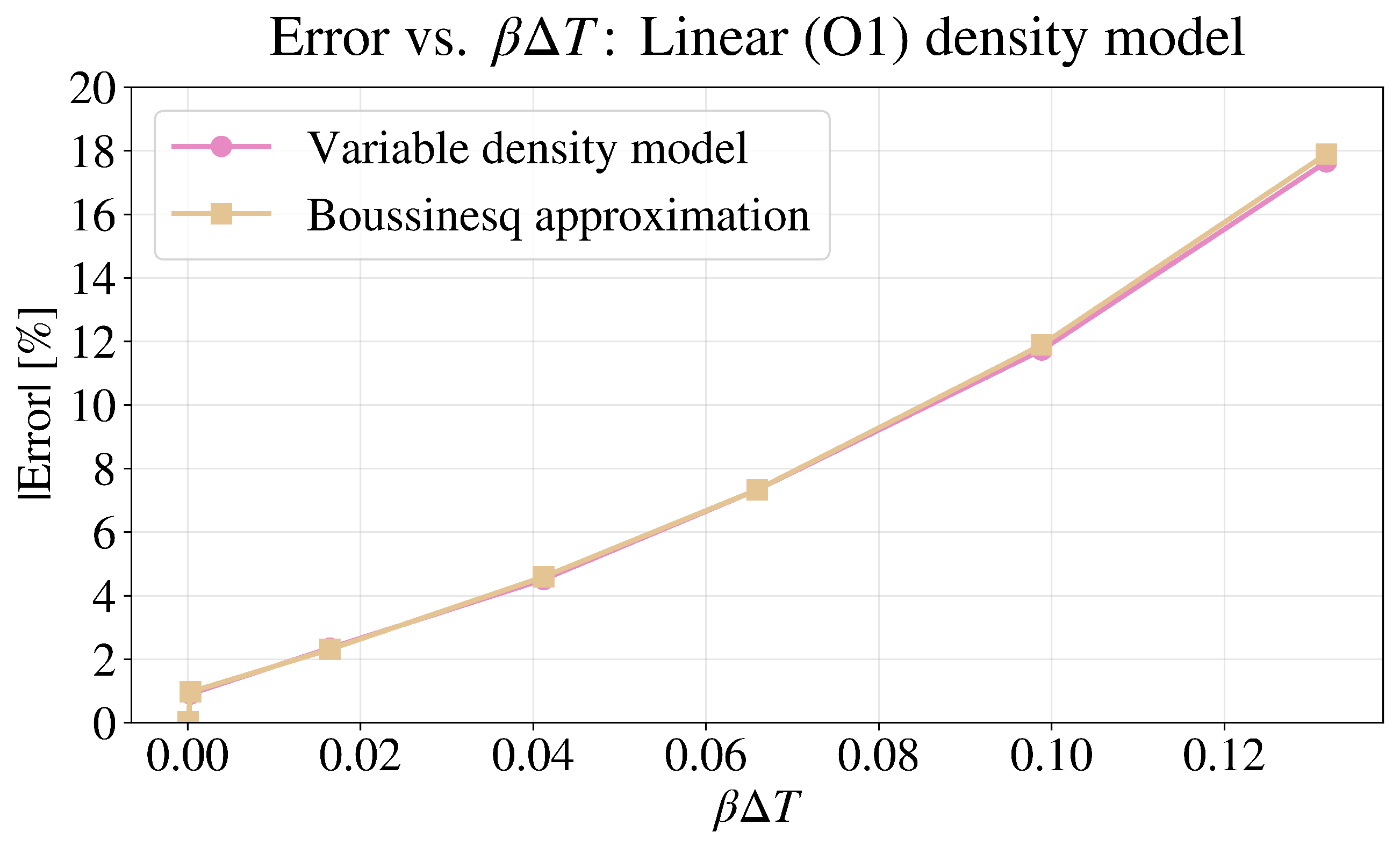
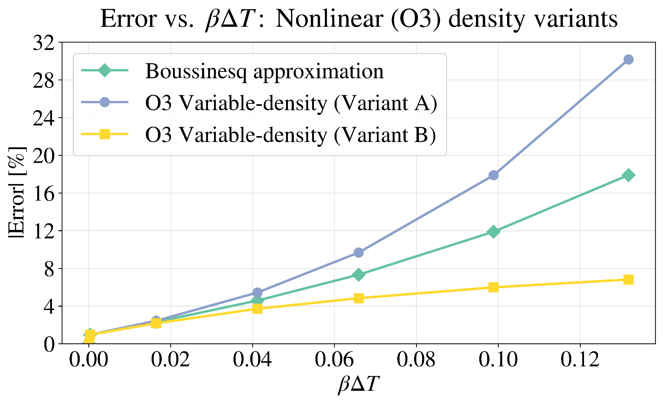
Figure 12 and Figure 13 present the deviations of the predicted average Nusselt number from the de Vahl Davis benchmark as a function of the nondimensional parameter $\beta \Delta T$ for the O1 linear density correlation and the two O3 nonlinear variants.

For the linear density correlation (Figure 12), the Boussinesq formulation and the full variable-density model yield nearly identical deviations over the entire range of $\beta \Delta T$. This behavior is expected, as discussed in Section 4.1: the Boussinesq approximation retains only the first-order term of the Taylor expansion of $\rho \left(T\right)$, which corresponds exactly to the O1 linear density model. As a result, both formulations produce identical buoyancy forces and therefore the same natural-convection behavior.

For the nonlinear O3 density correlations (Figure 13), the variable-density results progressively deviate from the linear trend as $\beta \Delta T$ increases, reflecting the growing influence of higher-order curvature in the density–temperature relationship. Variant A, which introduces negative curvature, causes density to decrease more rapidly with temperature than in the linear model. This leads to stronger buoyancy forces, enhanced convection, and higher Nusselt numbers. Consequently, the Boussinesq approximation underestimates convective heat transfer for this variant. In contrast, Variant B exhibits positive curvature, resulting in a slower decrease in density and therefore weaker buoyancy forces. In this case, the Boussinesq approximation overestimates the convective heat transfer.

Despite these opposite tendencies, the Boussinesq formulation yields identical predictions for both nonlinear variants because it retains only the linear term $\beta (T-T_{\mathrm{ref}})$ of the density expansion and is therefore insensitive to higher-order density variations.

It should be noted that the present assessment is based on a two-dimensional square cavity configuration, evaluated at a single Rayleigh number ($Ra={10}^3$) and for the KCl–UCl₃ molten-salt mixture. Therefore, the conclusions regarding the applicability of the Boussinesq approximation should be interpreted within the scope of this configuration.

A key outcome of this analysis is the establishment of a practical applicability criterion for the Boussinesq approximation. Because the approximation relies on linearizing the density field, the relevant nondimensional parameter is the relative density change,

$${\displaystyle \frac{\Delta \rho }{{\rho }_{\mathrm{ref}}}}=\beta \Delta T,$$

(28)

which corresponds to the first-order term of the Taylor expansion of $\rho \left(T\right)$. This parameter therefore represents the magnitude of density variations relative to the reference density and provides a direct measure of the validity of the linear density approximation used in the Boussinesq formulation.

As shown in Figure 13, noticeable deviations from the full variable-density solution emerge once $\beta \Delta T\gtrsim 0.1$, corresponding to a relative density variation of approximately 10%. This threshold is consistent with common engineering practice, in which density variations exceeding about 10% are generally considered beyond the valid range of the Boussinesq approximation. Beyond this limit, higher-order density effects become increasingly important and a fully variable-density formulation is required.

The results indicate that the Boussinesq approximation remains accurate for $\beta \Delta T\lesssim 0.1$, corresponding to relative density variations below approximately 10%. Although this threshold was identified using chloride-based molten-salt properties, the criterion itself is fundamentally fluid-independent. Therefore, the applicability limit obtained in this study is relevant not only for molten salts but also for other fluids undergoing buoyancy-driven natural convection.

Because the benchmark problem considered in this study is relatively simple, the computational cost difference between the full variable-density formulation and the Boussinesq approximation is negligible. However, for larger and more complex simulations with strongly temperature-dependent properties, the Boussinesq approach can offer computational advantages due to the simplified treatment of density in the momentum equations.

Although the present study considers a two-dimensional cavity configuration consistent with the classical de Vahl Davis benchmark, the governing equations and the validity criterion for the Boussinesq approximation are independent of dimensionality. Therefore, the applicability limit identified in this work is expected to remain relevant for three-dimensional buoyancy-driven flows, although realistic reactor geometries may exhibit additional three-dimensional flow structures.

5. Conclusions

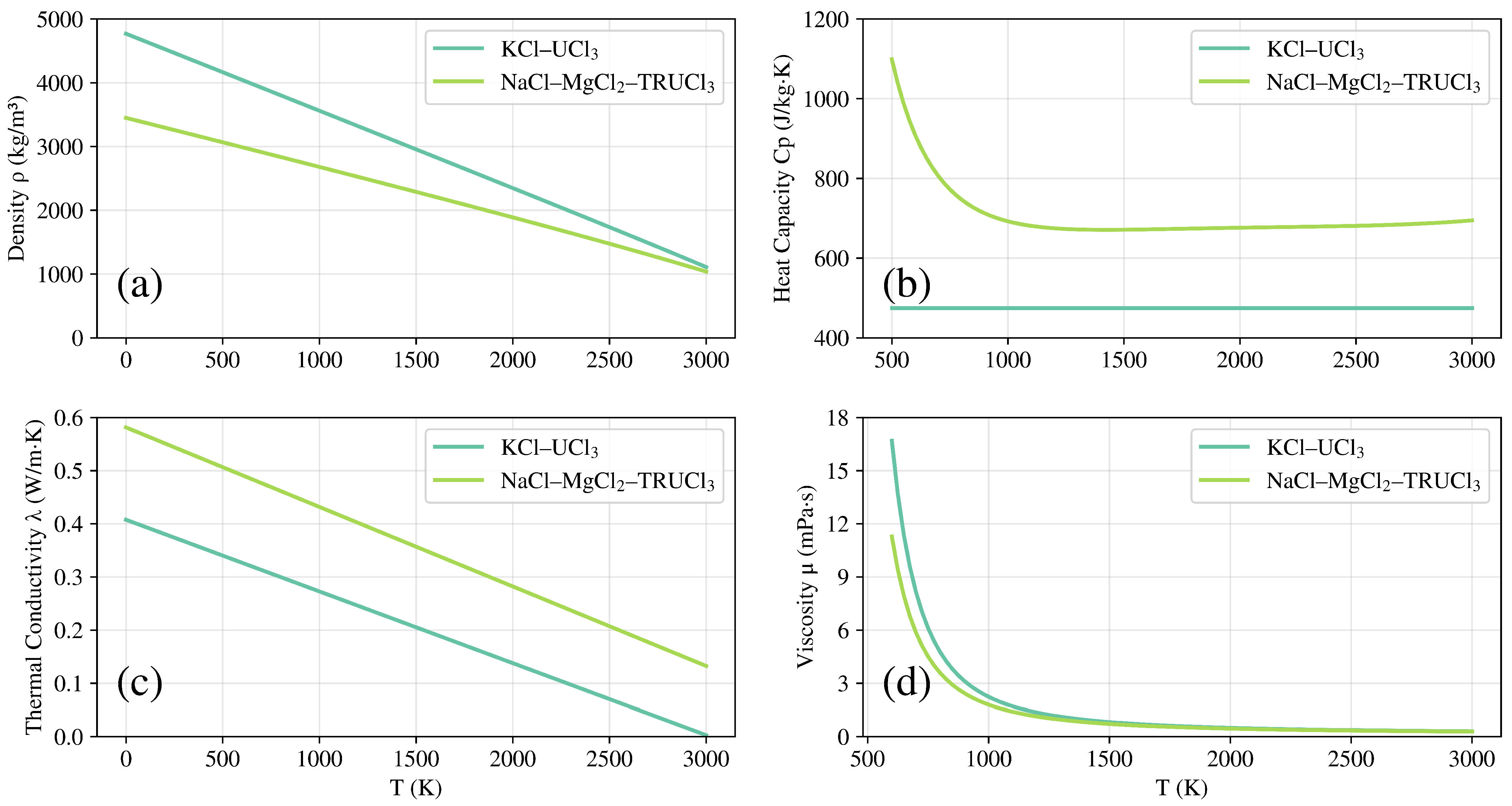
This work presented the development and verification of CUPID-MSR, an extended version of the CUPID thermal–hydraulic code incorporating the thermophysical properties of KCl–UCl₃ and NaCl–MgCl₂–TRUCl₃ molten-salt mixtures. Temperature-dependent correlations for density, specific heat capacity, thermal conductivity, and viscosity were implemented to represent realistic chloride-based molten-salt behavior.

The code was tested against the de Vahl Davis natural-convection benchmark for Rayleigh numbers between ${10}^3$ and ${10}^6$. The predicted average Nusselt numbers agreed with the reference benchmark within 0.4–3.9%, demonstrating the correctness of the numerical formulation, material property implementation, and boundary-condition treatment. The benchmark simulations also reproduced the characteristic flow structures reported in the literature, further supporting the physical realism of the simulations. Additional sensitivity studies showed that variations in reference temperature and temperature-dependent thermophysical properties do not adversely affect numerical stability or predictive accuracy, indicating that CUPID-MSR can reliably capture natural-convection behavior over a wide thermal range.

In addition to code verification, this study evaluated the applicability of the Boussinesq approximation by comparing it with the full variable-density formulation over a wide range of temperature differences. Using the nondimensional parameter $\beta \Delta T$, which corresponds to the relative density change $\Delta \rho /{\rho }_{\mathrm{ref}}$, a practical validity limit for the Boussinesq approximation was identified. The results indicate that the Boussinesq approximation remains accurate for $\beta \Delta T\lesssim 0.1$, while larger density variations lead to noticeable deviations that require a fully variable-density treatment. This threshold is consistent with classical criteria reported in the natural-convection literature and confirms their applicability for molten-salt thermophysical properties within the considered configuration.

Overall, this study provides the first systematic verification of the CUPID-MSR code for molten-salt applications, demonstrating that the well-established multi-dimensional thermal–hydraulic code CUPID has been extended to MSR systems, enabling its application to detailed simulations of emerging MSR concepts. In addition, it establishes a practical, fluid-independent criterion for the applicability of the Boussinesq approximation. These results contribute to the development of reliable computational tools for component-scale analysis of MSRs and support future high-fidelity simulations of MSR core thermal hydraulics.