


Abstract
Deep learning has become an important tool for wind power forecasting because it can help improve wind energy utilization and support reliable grid-connected operation. For wind farms, accurate turbine-level forecasting depends on spatial interactions among turbines and temporal evolution of historical operating data. In this study, a spatio-temporal forecasting framework is developed by combining a Graph Attention Network with a Temporal Convolutional Network. The graph attention module describes the neighborhood relations among turbines and learns their influence strengths adaptively, while the temporal convolution module extracts temporal patterns from multivariate SCADA sequences for multi-step prediction. On this basis, the learned attention weights are further used to define a node influence metric. This makes it possible to identify a small set of key turbines and use only their historical data to predict the future power output of the whole wind farm. The proposed framework is evaluated using one year of SCADA data from 134 turbines. A sliding-window dataset is constructed, and the model is tested on the training, validation, and test sets. The results show that the method can capture the spatio-temporal dependencies within the wind farm and still provide effective farm-wide forecasting when only limited observation nodes are available. The value of this work lies in organizing existing techniques around a practical wind farm forecasting task and in providing an interpretable prediction strategy based on key turbine selection, rather than in proposing a fundamentally new theoretical model.
1. Introduction
In 2024, the global cumulative installed capacity of wind power reached 1136 GW, marking an 11% increase from the previous year. The Global Wind Energy Council (GWEC) holds an optimistic attitude towards the further development of global wind power in the next decade [1]. Wind power is becoming an important global energy source. However, the inherent stochasticity of wind resources and the operational complexity of wind turbines introduce significant volatility and uncertainty into power output, presenting considerable challenges for grid scheduling, power control, and secure grid integration. Consequently, wind power forecasting methodologies have progressively shifted from physical and statistical models toward data-driven paradigms [2,3,4]. Traditional statistical approaches, such as ARIMA and Support Vector Regression (SVR), perform adequately with small datasets or under linear assumptions. Nevertheless, they often fail to capture the non-linear characteristics intrinsic to wind power time series or the spatial dependencies among turbines arising from wake effects, terrain variations, and operational control strategies.
In recent years, deep learning has gained substantial traction in wind power forecasting due to its superior feature extraction capabilities. Recurrent Neural Networks (RNNs), including variants like Long Short-Term Memory (LSTM) and Gated Recurrent Units (GRUs) [5,6], effectively model temporal dependencies, while Convolutional Neural Networks (CNNs) excel at extracting local temporal patterns. Attention-based architectures, particularly the Transformer, have demonstrated remarkable performance in long-sequence modeling. More recently, the Temporal Convolutional Network (TCN) has been increasingly adopted for wind power prediction, often integrated with attention mechanisms or decomposition–reconstruction strategies to better characterize multi-scale fluctuations [7].
From a spatial perspective, wind turbines within a farm exhibit pronounced spatial correlations due to wake effects, terrain roughness, and meteorological field propagation. Predicting farm-wide power output based solely on individual turbine histories fails to account for these couplings. To address this, some studies have employed spatio-temporal convolutional networks for joint multi-turbine prediction. Furthermore, Graph Neural Networks (GNNs), which represent non-Euclidean topological relationships through node–edge structures, have been extensively validated in power system applications, demonstrating their capacity to model complex dependencies [8]. In the context of wind turbine state prediction, incorporating domain knowledge constraints into GNNs has been shown to enhance interpretability and generalization [9]. Among GNN variants, the Graph Attention Network (GAT) is particularly well suited for capturing heterogeneous inter-turbine influences by learning adaptive attention weights for neighborhood aggregation [10].
For unified spatio-temporal modeling, the Transformer architecture offers parallel processing advantages and an alternative mechanism for capturing long-range sequence dependencies via self-attention [11,12,13,14]. Concurrently, systematic evaluations of TCNs have confirmed that architectures based on causal and dilated convolutions are highly competitive across diverse sequence modeling tasks while offering superior parallel training efficiency [13].
At the wind farm level, Wu et al. [15] proposed a deep learning framework that integrates high-resolution meteorological factors with physical constraints for short-term forecasting, exemplifying a data-driven approach that maintains physical consistency. Graph neural networks have also been employed to model couplings across both geographically dispersed farms and individual turbines within a farm. Huang et al. [16] developed a short-term forecasting method for multiple wind farms based on spatio-temporal global feature enhancement, constructing spatio-temporal graphs to facilitate information propagation and improve prediction robustness. Focusing on intra-farm dynamics, Qiu et al. [17] introduced a spatio-temporal graph neural network that accounts for wake shading effects, combining graph-based modeling with gated dilated convolutions to extract spatio-temporal features in parallel; experimental results on measured data confirmed its efficacy in improving multi-step-ahead predictions.
To address these issues, this study develops a spatio-temporal forecasting framework for wind farms by integrating a Graph Attention Network and a Temporal Convolutional Network. The GAT module is used to learn adaptive inter-turbine influence weights over a geographically constructed graph, while the TCN module models the temporal evolution of multivariate SCADA sequences for multi-step forecasting. Based on the learned attention distribution, node influence scores are further defined to identify key turbines and support sparse-input farm-wide prediction. Therefore, the contribution of this work lies mainly in the task-oriented integration of existing techniques and the development of an interpretable and practical forecasting strategy, rather than in a fundamental theoretical innovation.
2. Methodology
2.1. Dataset Construction and Preprocessing
The experimental dataset [18] comprises one year of 10 min resolution SCADA data from 134 wind turbines, along with the relative positions and altitudes of these turbines. To address the issues of temporal misalignment and missing values in the raw SCADA records, the starting time point was identified for each turbine, and the full-year time series was extracted accordingly. Missing values were annotated using a mask matrix to prevent invalid labels from interfering with the training process. Furthermore, wind direction was calculated based on the nacelle direction (Ndir) and the relative wind angle with respect to the nacelle (Wdir). Since the SCADA records do not directly provide the absolute wind direction, it is reconstructed from the nacelle yaw direction and the relative wind-direction angle. Let denote the nacelle direction measured clockwise from geographic north, and let denote the signed relative angle between the wind direction and the nacelle axis. Then, the absolute wind direction is computed as follows:
where denotes the angle normalization operator that maps the result into the interval .
Because wind direction is a circular variable, directly using its degree value would introduce an artificial discontinuity at . Therefore, the reconstructed wind direction is encoded as follows:
2.2. Graph Construction and Model Input
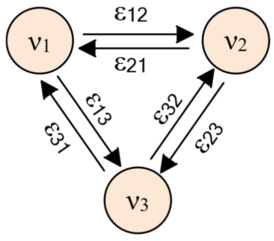
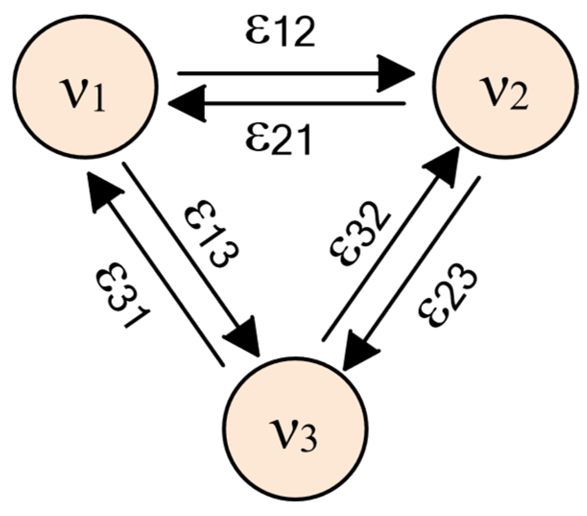
A directed graph is constructed based on the geographic positions of wind turbines within the farm, where each node represents an individual turbine, and a directed edge indicates the potential influence of turbine on turbine . The edge set is established using a combination of k-nearest neighbors (KNN) and distance thresholding according to the geographical coordinates of the turbines. To illustrate the node–edge influence relationships, Figure 1 presents an example of three geographically adjacent turbines and their corresponding graph structure.
Figure 1.
Diagram of Influence Relationships Among Adjacent Nodes.
For multi-step-ahead time-series prediction, the model input consists of multivariate feature sequences spanning a lookback window of time steps for all turbines in the farm, denoted as , where represents the number of input features per turbine. The corresponding output is the future active power sequence for all turbines over a prediction horizon of time steps, denoted as . The resulting graph provides a sparse and geographically meaningful neighborhood structure for subsequent spatial dependency modeling.
2.3. GAT–TCN Full-Input Teacher Model
A full-input model is first constructed to comprehensively capture the spatio-temporal dependencies among all wind turbines within the farm. In this configuration, the model performs time-series prediction for each node while simultaneously capturing spatial dependencies through the Graph Attention Network (GAT) mechanism.
For spatial dependency modeling, the Graph Attention Network (GAT) is employed to perform attention-based aggregation over node neighborhoods at each time step .
The attention coefficient represents the edge attention weight, which adaptively computes the influence strength between wind turbines; denotes the iteratively updated transformation matrix; represents the multi-dimensional vector at time step for node (neighboring node ) from the input multi-dimensional sequence mentioned earlier; and denotes the aggregated attention set vector of all neighboring nodes for node at time step .
For temporal dependency modeling, the Temporal Convolutional Network (TCN) is adopted, which consists of causal convolutions and dilated convolutions. It extracts multi-scale historical features in a parallel manner to achieve multi-step-ahead prediction.
2.4. Key Node Selection
After the full-input model is trained, the node influence is constructed using the attention set of the entire wind farm output by GAT. The attention matrices from several batch windows in the validation set are averaged across heads and batches to obtain , and the output influence of node is defined as follows:
This represents the average information contribution of node to all other nodes in the farm. The set of key wind turbine nodes is obtained by sorting in descending order, which will be used for subsequent sparse-input radiation experiments.
2.5. Farm-Wide Prediction via Observed Node Radiation
To validate whether farm-wide prediction can be supported by only a limited number of observed turbines, a sparse-input radiation prediction model is constructed. This setting uses the same graph connectivity structure as the full-input model, so that the spatial dependency pattern remains unchanged. The only difference is at the input stage: only the historical features of the selected key nodes are retained, while the inputs of all other nodes are set to zero. In addition, an observation indicator feature is appended to each node, where 1 indicates that the node is observed and 0 indicates that its original input features are masked out. Under this setting, farm-wide power prediction is generated through the learned spatio-temporal dependency propagation over the graph structure, using only sparse observations from the key turbines.
2.6. Evaluation Metrics
Masked weighted loss functions and evaluation metrics are employed during training and assessment to prevent interference from missing labels. The primary evaluation metrics include Mean Absolute Error (MAE) and Root Mean Square Error (RMSE), which are expressed as follows:
where represents the model’s predicted power values for wind turbines over a future horizon of time steps, denotes the corresponding ground truth values, is the mask matrix indicating valid data points, is the total number of valid data points after excluding missing values, and represents the Hadamard product operator.
3. Results and Analysis
3.1. Experimental Preprocessing
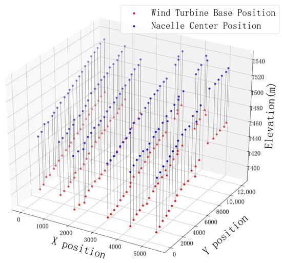
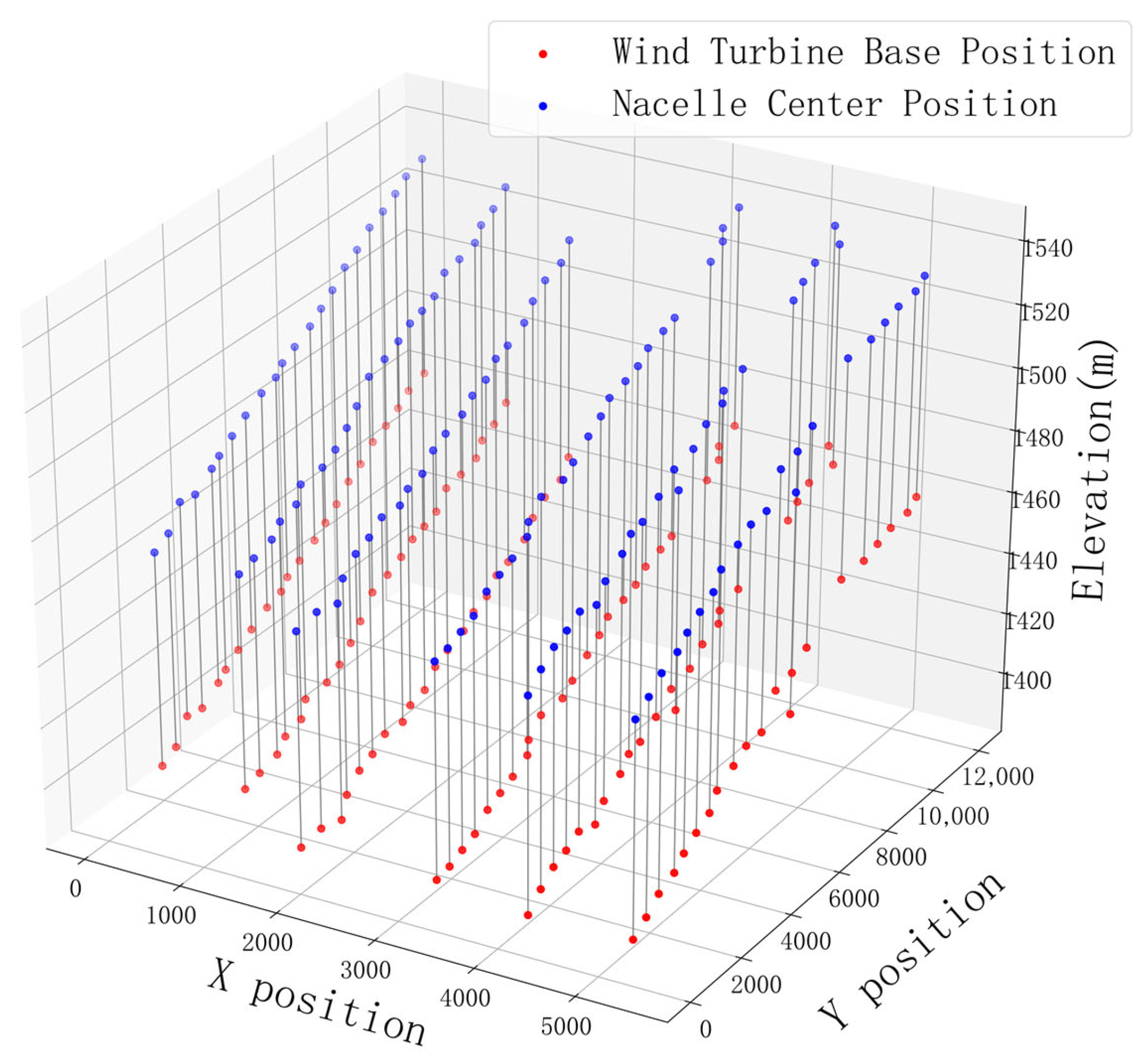
The dataset comprises a total of 134 wind turbines, with 10 min resolution data spanning from 1 January 2021, 0:00, to 31 December 2021, 23:50. After removing leading blank data, each turbine contains 52,559 rows of data for the entire year. The key information columns extracted include turbine ID, timestamp, active power, wind speed, yaw angle, and nacelle direction. Additionally, the location information for each turbine, including relative position and altitude, is extracted. Figure 2 illustrates the actual altitude and relative position distribution of the wind farm reconstructed from turbine locations.
Figure 2.
Schematic Diagram of Wind Turbine Distribution within Wind Farm.
For time-series forecasting, the input window is configured as a three-dimensional tensor , and the corresponding output window is (power only). The forecasting task is set as multi-step prediction, where all 36 time steps (representing the past 6 h) are used to predict the next 12 time steps (2 h ahead).
3.2. GAT and Full-Input Model Construction
First, a static KNN graph is constructed for all 134 wind turbines in the farm. The two-dimensional Euclidean distance is employed to measure spatial proximity between turbine locations. For any two nodes and representing wind turbines, the positional representation of the Euclidean distance is expressed as follows:
where and denote the X-axis and Y-axis coordinates on the plane, respectively. For each turbine, the nearest turbines are selected as its neighbor set, and directed edges are established accordingly.
Edge features are constructed on the directed edges, incorporating the two-dimensional Euclidean distance , the trigonometric representations of wind direction and , as well as the altitude difference . Additionally, for each existing edge , a reverse edge is added to enhance graph connectivity. Table 1 presents the parameter settings adopted for the spatial graph construction in this study.
Table 1.
Parameters for Graph Building.
After completing the KNN graph construction, time-series prediction is performed for all nodes using a parallel TCN framework with 134 branches corresponding to the number of nodes. The attention mechanism updates the influence coefficient weights on bidirectional edges during each training step.
For spatial modeling, the GAT adopts a single-layer architecture with a two-head attention mechanism. The hidden representation dimension for each attention head is 16, and the node representation dimension after spatial encoding is 32. An ELU non-linear activation function is applied, followed by a dropout layer with a rate of 0.1 to enhance training stability. Spatial encoding updates the spatial attention and neighborhood aggregation every three time steps within the input window. During forward propagation, the model outputs the spatial attention matrix and averages the updates across the window.
For temporal modeling, each individual TCN model employs three residual convolutional blocks with a channel dimension of 64. The convolution kernel size is set to 3, and the dilation factors for the dilated convolutions are configured as 1, 2, and 4. The hyperbolic tangent function (tanh) is adopted as the activation function, with a dropout layer of rate 0.1 applied after each convolutional layer. Cross-layer feature fusion is implemented through skip connections, where the outputs of each residual block are accumulated layer by layer to form the final temporal representation. For prediction, the feature at the last time step of the TCN output sequence is taken as input, mapped to the 12-step-ahead forecast through layer normalization and a two-layer fully connected prediction head.
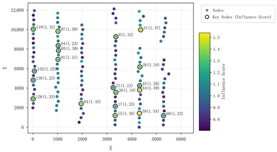
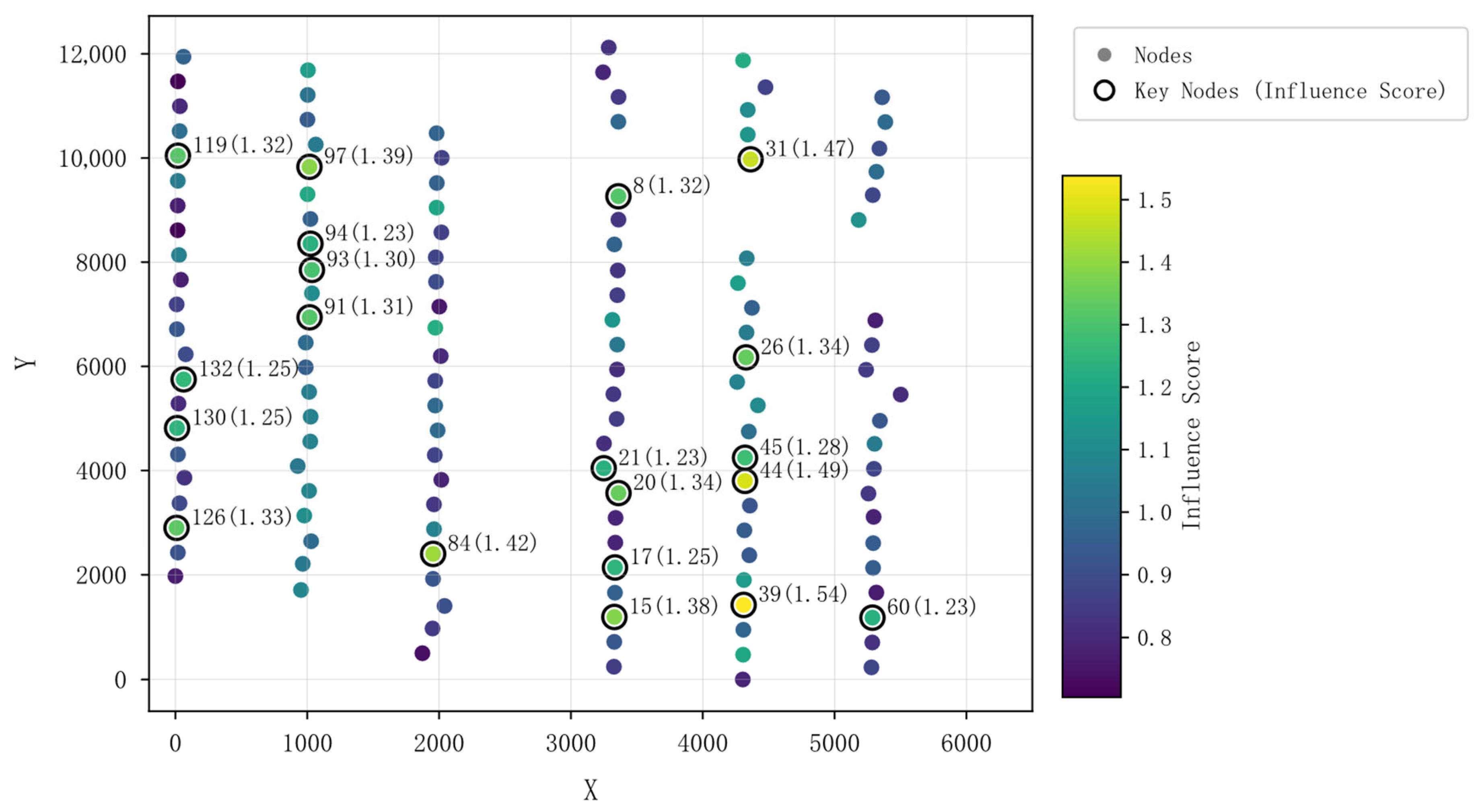
In the spatial dimension, the graph attention mechanism learns the mutual influence strengths among turbine neighborhoods, generating interpretable spatial attention weights. In the temporal dimension, the Temporal Convolutional Network extracts features from the historical sequences of each turbine, enabling multi-step-ahead power prediction for all nodes across the farm. The attention distributions are aggregated into node influence metrics, and key nodes with higher influence are selected. Figure 3 illustrates the distribution and influence coefficients of the top 20 key wind turbines ranked by outward influence. Based on this node ranking, the top 5, top 10, top 15, and top 20 lists of farm-wide nodes by outward influence are compiled as experimental foundations for subsequent sparse-input experiments.
Figure 3.
Diagram of Critical Influence Nodes.
3.3. Sparse-Input and Radiation Prediction Experiments
Sparse-input experiments are constructed based on the node outward influence ranking derived from the full-input model. A set of wind turbines is selected as key nodes according to descending influence, where represents different scales. The input tensor of sliding-window samples is sparsified by retaining only the historical feature sequences of key nodes, while the features of non-observed nodes are masked. Additionally, a one-dimensional observation flag is appended to the feature dimension to indicate whether a node is observed. Other model parameter configurations remain consistent with the full-input model design described above.
As a comparative experiment, independent time-series prediction is performed for the 20 key wind turbines using the same TCN model architecture described earlier. To enrich the baseline comparison, an STGCN baseline was additionally implemented under the same dataset, graph construction, and train/validation/test split settings. The model adopts stacked spatio-temporal convolution blocks composed of temporal convolution and graph convolution, and is trained using the same masked prediction objective for fair comparison. Table 2 and Table 3 presents the comparison of farm-wide prediction mean errors under different numbers of radiating nodes against the time-series prediction, and STGCN errors, with MAE and RMSE units in kW.
Table 2.
Research and Comparison of Experimental Error and Training Time.
Table 3.
Research and Comparison of Training Time.
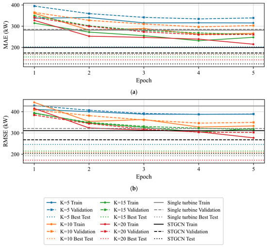
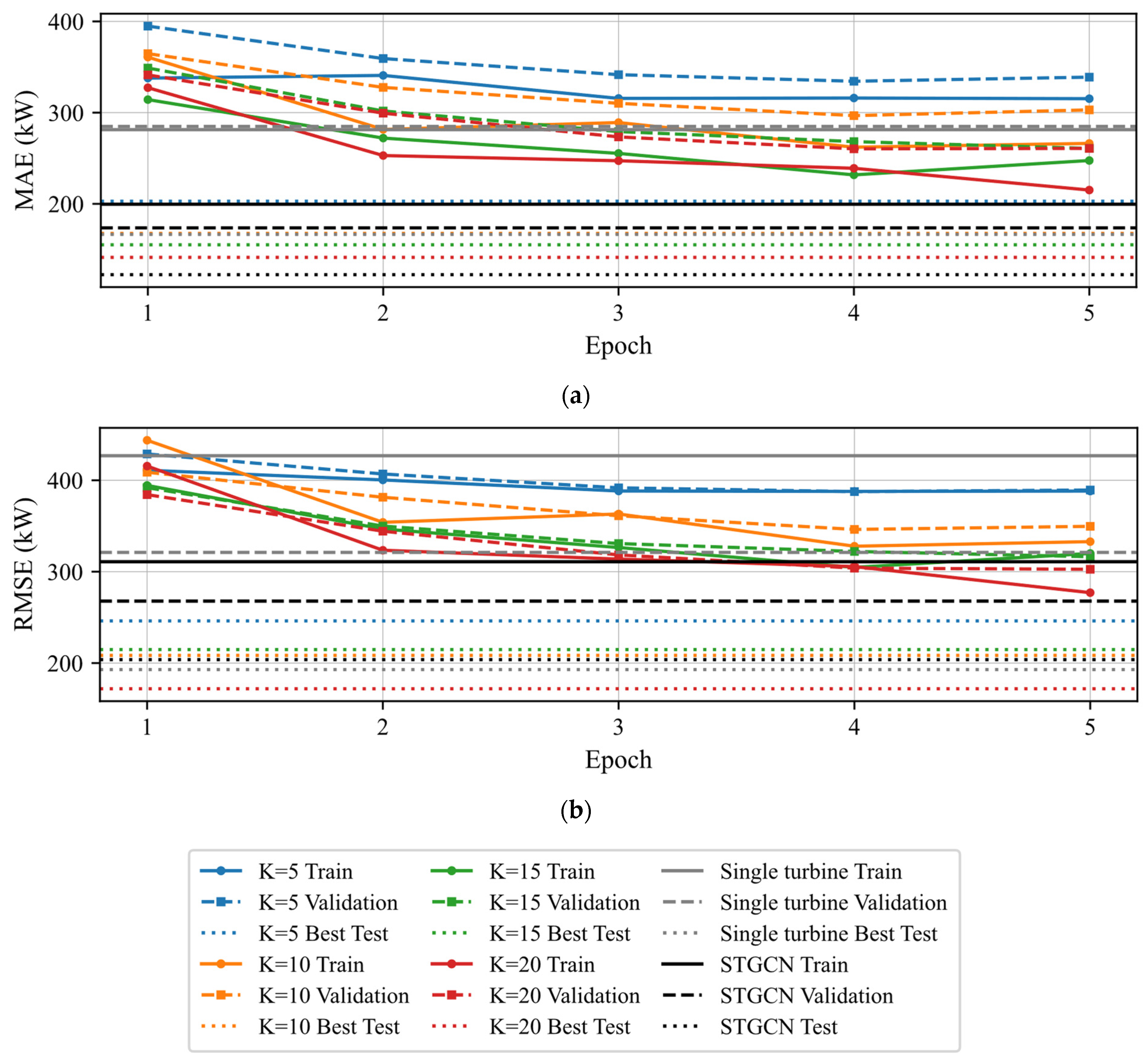
It can be observed that as the number of observed nodes increases, the overall performance of the proposed model shows a clear improvement trend. On the test set using the optimal model selected by validation RMSE, the MAE/RMSE decreases from 291.262/399.818 with to 221.651/334.601 with , indicating that increasing the number of key nodes enhances the model’s ability to characterize the state variations of all turbines in the farm, thereby reducing prediction errors. The comparison of MAE and RMSE is shown in Figure 4.
Figure 4.
Comparative Chart of Experimental Loss Error and Training Time in Research. (a) Comparison of MAE. (b) Comparison of RMSE.
Furthermore, the training and validation results generally show improved performance as the number of selected key turbines increases. In particular, when , both the validation error and the supplementary metrics exhibit a clearer and more stable improvement trend, indicating stronger generalization ability with more sufficient observational information. On the test set, the proposed radiation model consistently benefits from increasing , with MAE decreasing from 222.07 to 145.52, RMSE decreasing from 317.17 to 248.72, and increasing from 0.245 to 0.536 as rises from 5 to 20. The sMAPE also remains at a relatively stable level and reaches 1.190 at .
Compared with the single-turbine baseline, the proposed method with achieves better predictive performance, reducing the test MAE from 170.17 to 145.52 and the test RMSE from 310.48 to 248.72, while improving the test from 0.254 to 0.536. At the same time, its average training time per turbine is 98.01 s, which is lower than the 110.15 s required by STGCN. These results indicate that the proposed framework provides a practical trade-off among forecasting accuracy, observation cost, and computational efficiency. Therefore, it is particularly suitable for real wind farm scenarios in which complete farm-wide observations are difficult to obtain or expensive to maintain.
Under the current full-observation setting, STGCN achieves stronger predictive accuracy than the proposed method with . However, the proposed framework has a distinct advantage in terms of input sparsity. Specifically, STGCN relies on complete graph observations from all turbines, whereas the proposed method only requires a small number of key turbines as input nodes to support farm-wide forecasting.
Although the proposed method shows a certain reduction in predictive accuracy compared with STGCN, it still maintains acceptable forecasting performance under sparse-input conditions. When only twenty key turbines are used, the proposed method achieves a test MAE of 145.52, a test RMSE of 248.72, and a test R2 of 0.536. At the same time, its average training time per turbine is 98.01 s, which is lower than the 110.15 s required by STGCN. These results indicate that the proposed framework provides a practical trade-off among forecasting accuracy, observation cost, and computational efficiency. Therefore, it is particularly suitable for real wind farm scenarios in which complete farm-wide observations are difficult to obtain or expensive to maintain.
4. Conclusions
This study proposes a key node-based spatio-temporal forecasting framework for wind farm power prediction. First, a spatial graph structure is constructed according to the geographical neighborhood relationships among wind turbines. Then, a Graph Attention Network is used to learn the influence strengths between connected turbines, based on which node influence scores are derived to identify a small set of key turbines as observation nodes. In the temporal dimension, a Temporal Convolutional Network is employed to model historical multivariate SCADA sequences. By using only the historical information from selected key turbines as input and propagating information through the spatial structure, the proposed framework enables joint prediction of future power for all turbines in the wind farm.
The main contribution of this study lies in integrating graph attention-based influence learning, key node identification, and spatio-temporal forecasting into a unified and interpretable framework. In addition to farm-wide multi-step forecasting, the method also provides influence-based turbine rankings, which may support monitoring point deployment and sparse-observation forecasting in practical wind farm applications. Based on the experimental results, the main conclusions are as follows.
(1) Compared with the single-turbine baseline, the proposed method achieves better overall predictive performance. When twenty key turbines are used, the test set mean absolute error decreases from 170.17 to 145.52, the root mean square error decreases from 310.48 to 248.72, and the coefficient of determination increases from 0.254 to 0.536. These results indicate that introducing inter-turbine spatial dependency modeling is more effective than performing independent turbine-wise time-series forecasting.
(2) Increasing the number of selected key turbines generally improves forecasting performance. As the number of key turbines increases from five to twenty, the test set mean absolute error decreases from 222.07 to 145.52, the root mean square error decreases from 317.17 to 248.72, and the coefficient of determination increases from 0.245 to 0.536. The symmetric mean absolute percentage error remains relatively stable overall and reaches 1.190 when twenty key turbines are used. These results suggest that a larger set of key turbines provides richer observational information and improves farm-wide prediction accuracy.
(3) When the number of selected key turbines reaches ten or more, the validation performance becomes more stable and the generalization ability improves. The validation errors for ten, fifteen, and twenty key turbines show a clearer and more consistent decreasing trend, whereas the five-node setting still exhibits relatively high error levels. This indicates that excessively sparse observations are insufficient to fully capture the environmental and operational variations across the wind farm.
(4) Compared with STGCN, the proposed framework shows a different advantage. Under the current full-observation setting, STGCN achieves higher predictive accuracy. However, the proposed method requires only a small subset of key turbines as input, whereas STGCN depends on complete graph observations from all turbines. Therefore, the proposed framework provides a practical trade-off between forecasting accuracy, observation cost, interpretability, and computational efficiency.
(5) The proposed method also demonstrates competitive computational efficiency. The average training time per turbine is about 98.01 s when twenty key turbines are used, which is lower than that of the single-turbine baseline and comparable to that of STGCN. This suggests that the proposed sparse-input spatio-temporal framework does not introduce excessive computational burden while reducing the dependence on full wind farm observations.
In practical wind farm operation, the proposed framework can be applied in several scenarios. First, it can support farm-level power forecasting when only a subset of turbines are reliably observed, which is useful in cases of sensor failure, communication loss, or limited monitoring resources. Second, the identified key turbines and their influence rankings can provide references for monitoring point deployment and data acquisition planning. Third, the framework may assist dispatch support and operational decision-making by providing farm-wide prediction under sparse-input conditions.
It should be noted that the present study is validated on one wind farm dataset only. Although the proposed framework is expected to be applicable to other wind farms, its transferability to sites with different climatological conditions, topographic characteristics, and turbine density distributions has not yet been fully verified. In particular, wind farms under different prevailing wind directions, terrain complexity, and wake interaction patterns may exhibit different spatial dependency structures. Further validation on multiple wind farms is still required before broader practical generalization can be claimed.
Future work will focus on three directions. The first is to introduce dynamic graph construction that can better reflect changing wind direction and wake interactions. The second is to include more advanced spatio-temporal baselines and more systematic component-wise ablation studies. The third is to evaluate the proposed framework on wind farms with different environmental and structural characteristics, so as to further assess its robustness and transferability.
Author Contributions
Conceptualization, X.D. and J.W.; Methodology, T.Z. and J.W.; Software, T.Z. and Y.H.; Validation, S.L., J.W. and Y.H.; Formal analysis, J.W.; Investigation, Y.H.; Resources, X.D. and Y.H.; Writing—original draft, S.L. and T.Z.; Writing—review & editing, S.L. and T.Z.; Visualization, T.Z.; Supervision, S.L. and X.D.; Project administration, X.D.; Funding acquisition, X.D. and J.W. All authors have read and agreed to the published version of the manuscript.
Funding
This research was funded by National Natural Science Foundation of China, grant number 52130607. National Natural Science Foundation of China, grant number 52366009, and Lanzhou Youth Science and Technology Talent Innovation Project, grant number 2025-QN-078.
Data Availability Statement
The original contributions presented in this study are included in the article. Further inquiries can be directed to the corresponding author.
Conflicts of Interest
The authors declare no conflicts of interest.
Abbreviations
| Abbreviation | Full Term |
| GWEC | Global Wind Energy Council |
| ARIMA | AutoRegressive Integrated Moving Average |
| SVR | Support Vector Regression |
| RNN | Recurrent Neural Network |
| LSTM | Long Short-Term Memory |
| GRU | Gated Recurrent Unit |
| CNN | Convolutional Neural Network |
| GNN | Graph Neural Network |
| GAT | Graph Attention Network |
| TCN | Temporal Convolutional Network |
| STGCN | Spatio-Temporal Graph Convolutional Network |
| KNN | K-Nearest Neighbors |
| SCADA | Supervisory Control and Data Acquisition |
| MAE | Mean Absolute Error |
| RMSE | Root Mean Square Error |
| sMAPE | symmetric Mean Absolute Percentage Error |
| ELU | Exponential Linear Unit |
References
- Global Wind Energy Council. Global Wind Report 2024; Global Wind Energy Council: Brussels, Belgium, 2025; Available online: https://www.gwec.net/reports/globalwindreport/2024 (accessed on 29 March 2026).
- Si, Y.X.; Liu, X.Q.; Su, X.J.; Tian, S.X. A review of offshore wind power forecasting research. Zhejiang Electr. Power 2025, 44, 60–71. [Google Scholar]
- Tang, X.Z.; Gu, N.W.; Huang, X.Q.; Peng, R.T. Progress on short-term wind power prediction technologies. J. Mech. Eng. 2022, 58, 213–236. [Google Scholar]
- Han, Z.F.; Jing, Q.M.; Zhang, Y.K.; Bai, R.Q.; Guo, K.M.; Zhang, Y. A review of wind power forecasting methods and new trends. Power Syst. Prot. Control 2019, 47, 178–187. [Google Scholar]
- Kazmi, S.; Gorgulu, B.; Cevik, M.; Baydogan, M.G. A concurrent CNN-RNN approach for multi-step wind power forecasting. arXiv 2023, arXiv:2301.00819. [Google Scholar]
- Souhe, F.G.Y.; Mbey, C.F.; Kakeu, V.J.F.; Meyo, A.E.; Boum, A.T. Optimized forecasting of photovoltaic power generation using hybrid deep learning model based on GRU and SVM. Electr. Eng. 2024, 106, 7879–7898. [Google Scholar] [CrossRef] [Scilit]
- Zhu, J.; Su, L.; Li, Y. Wind power forecasting based on new hybrid model with TCN residual modification. Energy AI 2022, 10, 100199. [Google Scholar] [CrossRef] [Scilit]
- Sejan, M.A.S.; Rahman, M.H.; Aziz, M.A.; Hameed, I.; Islam, M.S.; Sabuj, S.R.; Song, H.-K. Learning robust node representations via graph neural network and multilayer perceptron classifier. Mathematics 2026, 14, 680. [Google Scholar] [CrossRef] [Scilit]
- Veličković, P.; Cucurull, G.; Casanova, A.; Romero, A.; Liò, P.; Bengio, Y. Graph attention networks. In Proceedings of the International Conference on Learning Representations ICLR, Vancouver, BC, Canada, 30 April–3 May 2018. [Google Scholar]
- Vaswani, A.; Shazeer, N.; Parmar, N.; Uszkoreit, J.; Jones, L.; Gomez, A.N.; Kaiser, Ł.; Polosukhin, I. Attention is all you need. In Advances in Neural Information Processing Systems 30; Guyon, I., Luxburg, U.V., Bengio, S., Wallach, H., Fergus, R., Vishwanathan, S., Garnett, R., Eds.; Curran Associates, Inc.: Red Hook, NY, USA, 2017; pp. 6000–6010. [Google Scholar]
- Tian, C.; Xia, M.; Yuan, S.; Wang, L.; Zhuang, W. STGCformer: Spatio-temporal graph convolutional transformer for short-term wind power forecasting. Energies 2026, 19, 1214. [Google Scholar] [CrossRef] [Scilit]
- Liu, L.; Chen, H.; Shao, W.; Yang, Y. A hybrid Transformer–BiLSTM-based modeling method for photovoltaic modules. Energies 2026, 19, 962. [Google Scholar] [CrossRef] [Scilit]
- Bai, S.; Kolter, J.Z.; Koltun, V. An empirical evaluation of generic convolutional and recurrent networks for sequence modeling. arXiv 2018, arXiv:1803.01271. [Google Scholar] [CrossRef] [Scilit]
- Bispo Junior, D.A.; Leite, G.d.N.P.; Droguett, E.L.; de Souza, O.V.C.; Lisboa, L.A.; Cavalcanti, G.D.d.C.; Ochoa, A.A.V.; Costa, A.C.A.d.; Vilela, O.d.C.; Brennand, L.J.d.P.; et al. Short-Term Wind Power Forecasting with Transformer-Based Models Enhanced by Time2Vec and Efficient Attention. Energies 2025, 18, 6162. [Google Scholar] [CrossRef] [Scilit]
- Wu, Y.; Wang, B.; Chen, Y.; Jiang, H. Application of Deep Learning Model Integrating Refined Meteorological Factors and Physical Constraints in Short-term Wind Power Prediction. Power Syst. Technol. 2024, 48, 1455–1468. [Google Scholar]
- Huang, N.; Li, B.; Sun, H.; Wang, Y.; Cai, G.; Zhang, L. Short-term Prediction of Wind Power in Wide-area Multi-wind Farms With Enhanced Time-space Characteristics. Power Syst. Technol. 2025, 49, 3688–3698. [Google Scholar]
- Qiu, H.; Shi, K.; Wang, R.; Zhang, L.; Liu, X.; Cheng, X. A novel temporal–spatial graph neural network for wind power forecasting considering blockage effects. Renew. Energy 2024, 227, 120526. [Google Scholar] [CrossRef] [Scilit]
- Zhou, J.; Lu, X.; Xiao, Y.; Tang, J.; Su, J.; Li, Y.; Liu, J.; Lyu, J.; Ma, Y.; Dou, D. SDWPF: A dataset for spatial dynamic wind power forecasting over a large turbine array. Sci. Data 2024, 11, 469. [Google Scholar] [CrossRef] [Scilit] [PubMed]

Disclaimer/Publisher’s Note: The statements, opinions and data contained in all publications are solely those of the individual author(s) and contributor(s) and not of MDPI and/or the editor(s). MDPI and/or the editor(s) disclaim responsibility for any injury to people or property resulting from any ideas, methods, instructions or products referred to in the content. |
© 2026 by the authors. Licensee MDPI, Basel, Switzerland. This article is an open access article distributed under the terms and conditions of the Creative Commons Attribution (CC BY) license.