


Abstract
This manuscript presents an energy management strategy (EMS) for a commercial smart building participating in a tertiary frequency regulation market. The building integrates non-controllable components, such as loads and photovoltaic generation, and controllable resources such as a battery storage system and a set of electric vehicle (EV) chargers that are available for customers of the smart building. The EMS is based on model predictive control due to its innate ability to deal with operational constraints and different optimization criteria, which are critical for the operation of the EMS, and consists of two stages. The first iteratively optimizes energy costs and revenues from tertiary regulation reserves and activations in order to determine the optimal operation of the smart building and the regulation offers in nominal conditions. Then, a second problem determines the operation whenever an activation request is made. Simulation-based analyses are performed to study the performance of the EMS and its financial viability in diverse scenarios relevant to the smart commercial building. The results show that profits are greater if both upward and downward regulation can be provided, for a larger number of EVs and chargers and for longer connection times. Most notably, incomes from regulation almost match operation costs for a large number of chargers and EVs (240), obtaining a deficit of only EUR 39.12 for a day of operations.
1. Introduction
Our society faces a critical challenge due to elevated concentrations of greenhouse gases, and although global emissions have shown a slight decrease since 2019, their levels are still of great concern [1], with the energy and transportation being sectors the primary contributors to this issue [2]. To address this, many countries have implemented decarbonization policies, including fostering the incorporation of renewable energy sources (RESs) to the energy matrix and the progressive electrification of ground transportation [3,4].
Although the growing penetration of RESs and the rapid adoption of electric vehicles (EVs) represent significant environmental advances, these pose significant challenges for the electric grid. The inherent variability and forecasting uncertainty of RESs makes it difficult to maintain the supply–demand balance, while the widespread adoption of EVs changes the consumption patterns and introduces new demand peaks. Without proper management, both factors could greatly affect the stability and reliability of the electric grid. In this context, distributed energy resources (DERs) with storage capacity, such as battery energy storage systems (BESSs) and EVs themselves, emerge as key solutions against these issues.
The potential of these DERs goes beyond storage and local energy consumption. Both BESSs and EVs equipped with vehicle-to-grid (V2G) technologies can actively interact with the electric grid, dynamically adjusting their consumption or supply. This flexibility enables their use in energy markets or for providing ancillary services, thus contributing to the stability of the power system [5,6]. The growing integration of renewable generation and the gradual phase-out of rotating machines has increased the demand for ancillary services, especially those related to frequency regulation [7,8]. In this context, DERs are emerging as promising candidates to provide primary (automatic, fast, and brief), secondary (automatic, fast, and sustained over longer periods), and tertiary (manual, slower, and longer lasting) control [9]. For this reason, researchers have explored the use of DERs, such as BESSs and EVs, to provide frequency regulation services. BESSs present fewer operational constraints than EVs due to their exclusive purpose as energy storage systems (ESSs), which facilitates their participation in primary, secondary, and tertiary regulation services. For example, the authors of [10] propose an optimization model based on genetic algorithms to provide spinning reserves (primary regulation). Similarly, the works of [11,12] present optimization-based methods for regulation in the context of European ancillary service markets; while [11] deals with automatic frequency restoration reserves (aFRRs) and manual frequency restoration reserves (mFRRs), corresponding to tertiary regulation, Ref. [12] handles mFRR. These studies confirm the technical feasibility of BESSs to participate in all aforementioned levels, but Refs. [11,13] suggest that the initial investment remains high.
Unlike BESSs, EVs are not dedicated exclusively to energy storage, as their primary function is transportation. Charging stations aggregating a large number of EVs, then, by leveraging the flexibility in the charging operations of the batteries of EVs, can represent an alternative requiring lower initial investments to participate in the frequency regulation markets [14]. The feasibility of using EVs to provide regulation services depends mainly on the uncertainty associated with their usage, on the technologies available in the EVs, and the charging equipment. Initially, studies of EV usage were focused on unidirectional services [15]. Nevertheless, the adoption of vehicle-to-grid (V2G) technologies has motivated a drift towards investigations dealing with bidirectional services [16]. The majority of the existing literature focuses on secondary regulation [16,17,18,19,20]. In contrast, the participation of EVs in tertiary regulation has received considerably less attention. This alternative is particularly attractive in charging stations where the EVs are not used for prolonged periods for their primary transportation goal, e.g., private-use EVs with long dwelling times as opposed to those in transportation fleets with tighter mobility constraints. To the best of the authors’ knowledge, only a limited number of works have addressed EV participation in tertiary regulation [21,22]. However, both works deal with the management of EV charging, not addressing V2G capabilities. The work of [21] proposed a heuristic to enable fast computation and does not consider minimum bid sizes. The work of [22] proposes an optimization-based decision-making scheme, and considers a local energy communnity that participates in the provision of regulation services via a balancing market aggregator.
Besides the type of regulation service, existing works differ in the features of the decision scheme. While some approaches to manage the provision of regulation services using EV fleets choose to use heuristics, aimed primarily at small operators [21,23], most research has focused on optimization-based schemes motivated by financial considerations, typically balancing energy costs and regulation incomes subject to the system dynamics and operational constraints. Most works adopt a single time scale to account for the planning of EV charging, load dynamics, and regulation services [18,19,20,21,22]. However, the work of [17] considers a linear optimization model with two temporal scales: one with a small sampling time to manage EV charging, and another with larger sampling times to manage secondary regulation reserves. Stochasticity can also be considered in several manners, such as with scenario characterization of the uncertain variables emerging from the regulation services [18,19,20] or using explicit probability-based characterizations for the AGC signal [17]. Furthermore, some works adopt an approach based on model predictive control (MPC) for the energy management system (EMS) and regulation service participation [24,25]. MPC is also a control approach based on optimization, but the work in question specifically highlights a scheme based on repeated online optimization, enabling control decisions to be continuously updated as new state measurements and forecasts become available. This feature makes MPC especially well suited for systems with evolving operating conditions, tight constraints, and interacting time scales, such as those present in EV charging stations participating in grid services.
In this context, the present study focuses on the formulation of an EMS based on online optimization according with the MPC paradigm, for a commercial smart building equipped with PV generation, a BESS, and an EV charging station with V2G capabilities, which participates in tertiary frequency regulation markets by submitting regulation reserve offers and providing these when requested. The MPC management scheme iteratively solves an optimization in receding horizon fashion, taking into account the updated state of the system and reacting to uncertain regulation requests, minimizing the energy cost and maximizing profits from tertiary regulation. The proposed EMS has the following features: (i) The proposed EMS consists of two stages at each hour: first, the nominal operation of the smart building and the regulation reserve offers are computed; second, only if the offers are requested, the optimal operation of the smart building is determined while providing the regulation reserve. (ii) Two time scales, one associated with the internal operation and the other with regulation services, are considered. (iii) The probabilities of frequency regulation activations are computed from historial data and are incorporated in the objective functions. To analyze the proposed EMS, a detailed simulation study that considers different EV utilization profiles typical of commercial buildings is performed. Both the qualitative behavior of the management scheme and quantitative results regarding potential costs and incomes of the system are analyzed so as to provide guidelines for decision makers.
As discussed above, this is one of the few EMSs that have been developed for tertiary frequency regulation with EV participation. Compared with the previous works in the literature, most importantly, this is the first work that proposes an optimization-based EMS for tertiary regulation that deals with the V2G paradigm and considers direct participation of the operator in the regulation market, without going through an intermediate aggregator, and considering minimum bid constraints. The latter makes the optimization problem mixed-integer. Furthermore, this is the first work, to the best of the authors’ knowledge, that deals specifically with commercial buildings equipped with EV charging stations participating in tertiary regulation, and performs a financial analysis for this case. Other features not present in the previous literature on the topic are the use, for the entire prediction horizon, of two time scales and the possibility of optimizing the charging/discharging power of the EV batteries.
This manuscript is organized as follows: Section 2 presents the system, descrESSibes the problem, and establishes the considerations under which the management strategy will be designed; Section 3 presents the proposed strategy based on MPC, with a focus on the mathematical formulation of the associated optimization problem; Section 4 describes a case study with different scenarios, and presents and analyzes simulation results; finally, Section 5 synthesizes the main findings and suggests future research topics.
2. Problem Description
Large commercial buildings can integrate RESs and BESSs to reduce grid consumption and reduce operational cost. Likewise, the increasing adoption of EVs has driven the installation of EV supply equipment (EVSE) in the parking lots of these buildings, acting as an enabling factor for the transition towards smart buildings, characterized by an automated and integrated management of their energy resources [26]. This paradigm, besides increasing the internal efficiency, enables an active participation in ancillary services such as frequency regulation, which may provide economic benefits to the building operation. The main challenge consists of the simultaneous coordination of energy consumption and reserves for the regulation services, through the controllable resources, without compromising the primary building operation nor user satisfaction.
The system considered in this work is a commercial building connected to a grid that possesses photovoltaic (PV) generation, BESSs, and EVSE infrastructure. Figure 1 illustrates the proposed configuration: (i) non-controllable loads, including the building power demand and generation of the PV system; and (ii) controllable devices, including the BESS and N EV chargers for customers of the charging station.
Figure 1.
Power flow diagram of the smart commercial building.
Non-controllable elements are considered as known input data: the building demand (), which includes lightning and climatization, amongst other elements; and PV generation (). Controllable elements, on the other hand, can have their consumption/injection manipulated by the modulation of their bidirectional power flows. Although the storage dynamics of BESSs and EVs are similar, there are key differences in their operation.
The BESS is a dedicated resource with a storage and power charge/discharge ( for charging) that is always available to the system, except for operational constraints for power flows and stored energy. There are maximum power flows for charge and discharge. The available energy is represented by the state of charge (SOC) of the BESS (). It is an adimensional quantity that represents the fraction of energy available with respect to its capacity, and it must be kept within minimum and maximum values to prevent damage due to overcharging or undercharging.
On the other hand, the manipulation of the power charge/discharge of each EV ( for charging) is only available when they are connected to the EVSE. This infrastructure is assumed to be composed of several homogeneous chargers with V2G technology, enabling bidirectional interaction with the grid. The available energy is represented by the SOC of EV batteries (). In order to characterize heterogeneous customer groups (commercial clients and employees, amongst others), different connection profiles are considered. For each profile, an arrival time, a departure time, and a minimum required SOC level at the disconnection time are assumed known. This required SOC level is associated with the primary function of the battery, which is transportation. As for the BESS, there are maximum power flows for charge and discharge and minimum and maximum SOC values for each EV.
The demand that cannot be satisfied by internal generation/injection is imported from the grid and is denoted by (consumption is associated with a positive value). It is assumed that excedents are not sold to the grid, and therefore positive powers only () are considered.
The smart building participates in the manual ancillary service of mFRR, corresponding to tertiary frequency regulation. It is characterized by hourly power reserves with manual activation lasting up to 1 h, significantly more than what is required in primary and secondary regulation. This study assumes a market where reserves are offered dynamically at each hour, rather than day-ahead as in traditional markets. This approach responds to the growing penetration of RESs, which might render day-ahead planning impractical, and is particularly well suited for flexible resources such as EVs, whose behavior involves inherent uncertainties. The offers are bidirectional (can include both upward and downward power reserves), may be asymmetrical (different offers for upward and downward reserves), and must be larger than a threshold (100 kW in this study, motivated by the CAISO market [17]). The upward reserves represent a capacity to decrease consumption (which is similar to increase injected power), whereas downward reserves correspond to the capacity to increase consumption. It is assumed that it is a competitive market valued at marginal price, so that bids are immediately accepted. Upon acceptance, there are three possible scenarios: (i) no reserve activation, (ii) upward reserve activation, and (iii) downward reserve activation. In case the grid operator performs a manual request for reserve activation, the system needs to deploy the bid reserve for the remainder of the hourly block. For this reason, offers must be feasible both in terms of power and energy. There are payments associated with reserved capacities and additional payments for reserve activations.
The objective of the management strategy is to minimize the operational costs of the smart building, taking into account energy costs as well as profits due to participation in tertiary regulation, and to guarantee the satisfaction of operational constraints. In order to assess potential revenues, the hourly probabilities of reserve activations and are available, obtained from historical records.
3. Energy Management Strategy
3.1. Model Predictive Control Based Strategy
The participation in a tertiary regulation market with hourly offers requires an algorithm that combines immediate reaction ability with minding of long-term costs. To this end, an MPC-based energy management system is proposed, which is based on the hourly solution of optimization problems that determine the operation of the smart building. The high-level scheme of the strategy is presented here, and the details of the optimization are presented in the following subsections.
The overall strategy considers two optimization problems: the reserve bidding problem and the reserve activation problem. Both problems consider two temporal discretization scales: an inner scale associated with time index k, which has a time step of min and determines the dynamics of the smart building, especially the voltages in the batteries and all power flows; and the time index h, which has a time step of h, determines hourly reserves, and is the actual sampling time of the strategy. A prediction horizon of 24 h is considered, thus providing appropriate anticipation capacity to the decision scheme. The objective function accounts for the cost of the bought energy and the incomes associated with regulation reserves and provisions. The constraints include the storage dynamics of the BESS and EVs as well as operational constraints of the physical infrastructure and of market requirements. The reserve activation problem also includes constraints associated with complying with the effective provision of the requested regulation. Therefore, both problems aim to determine operation plans for the power flows and regulation reserves that minimize costs over 24 h while satisfying operational constraints. However, they will be used at different stages.
Let , with , denote the domain of time k, with a time step of min, such that refers to the current time and refers to 24 h ahead. Likewise, let , with , denote the domain of time h with a time step of h, such that refers to the current/first hour and refers to 24th hour. The times k and h are in sets and . In addition, denotes all time instants k contained in hour h. The set of EVs is denoted by .
In compact form, both optimization problems can be written as
This problem is a mixed-integer quadratic program MIQP, according to the cost function and constraints to be presented in detail in the following subsections.
The decision variables are organized into two vectors. The first one
considers all the power flows defining the operation of the system, in the time domain k, if no regulation action is performed: the power flow drawn from the grid, , of the BESS, , and of each EV, . We will refer to these as nominal power flows. The dynamics of the system are described by these variables in the time domain k. The second vector
includes the offered regulation reserves, ; the contributions to the offered reserves of the BESS and the EVs in the discretization time h where the regulation offers are performed, ; and the potential contributions of the BESS and the EVs in the discretization time k, given by . The discrete times k and h are coupled by the facts that: (i) regulation contributions at each time h are bounded by the potential contributions at each ; and (ii) the operational constraints are checked at each time k, and in particular, SOC constraints are checked, assuming regulation offers are provided as defined at each h.
At each hour, the reserve bidding problem is solved, which is given by (1) (without the activation constraints). The relevant outputs of this problem are the capacities and , which the smart building commits to the grid operator for the current period of 1 h, and the nominal operation plan including for all EVs and all instants k associated with the first hour of operation ().
The bid submission, in general, may or may not be accepted. In practice, if it is not accepted, a new problem has to be solved to define the optimal operation for the next hour without regulation reserves, but these will be considered from the second hour onwards. Based on the aforementioned assumptions (of marginal pricing) and in order to simplify presentation, from this point onwards, it will be assumed that the bid submission is accepted.
If the operator does not request activation of the regulation reserve, the smart building executes the nominal operation plan unchanged for 1 h, and the payment associated with capacity reserve is recorded. If, on the other hand, the reserve activation is requested during that hour block, the offered regulation has to be delivered and payments will come from the regulation reserves and provision. For defining the optimal operation in this case, the reserve activation problem is solved. This problem is given by (1) with the activation constraints, which enforce that the requested regulation is provided for the current hour, i.e., they set (or ) to be equal to the requested upward (downward) activation, set to zero the non-activated regulation, and set , to be equal to the declared (nominal) consumption for the first hour, so that the actual consumed power from the grid and by each component is
in the case of upward regulation, and
in the case of downward regulation. No constraints are imposed over the nominal operation plan or regulations for the remaining 23 h as they have not been committed; indeed, the plans may be adjusted (compared with those computed in previous instants) once the regulation is effectively provided.
The operation plans are implemented for the corresponding 1 h block only, and future operation decisions are determined by the upcoming optimizations to be solved in the following hours using the updated measurements of the system state. This corresponds to a closed-loop operation, thus providing robustness to operational uncertainty. Figure 2 illustrates the scheme described above: sensors provide the current state of the system, the optimizer defines a reserve bid and an operation plan, and whenever a reserve is accepted, an activation plan is recalculated and the system operates accordingly.
Figure 2.
Block diagram of the proposed EMS.
This scheme is further illustrated in Figure 3, which shows how the system responds to a power reserve bid made at 15:00 h, in three scenarios: no reserve activation, upward activation, and downward activation. More specifically, the plots show consumed power from 00:00 h to 15:00 h (which, indeed, is the same in the three scenarios), until the regulation reserves committed from 15:00 h until 16:00 h are considered. The upper plot shows the nominal planned consumed power (continuous line) and the corrections that would be made if downward (dashed line) or upward (dotted lines) regulation reserves are activated. The darker shaded area shows the 1 h block associated with the 15:00 h reserve. If no activation occurs, the system will continue operating according to . On the other hand, in the case of an upward (downward) activation, the consumed power is modified to that corresponding to the dotted (dashed) line in the first plot. The lighter shaded area shows that the plan determined for 16:00 h and onwards is different in the three scenarios due to the different decisions made at 15:00 h.
Figure 3.
Power consumption profiles associated with reserve capacity commitment and activation at 15:00 h: (a) projected power consumption including committed regulation reserves, as obtained from the reserve bidding problem; (b) power consumption with upward reserve activation, as computed by the reserve activation problem; and (c) power consumption with downward reserve activation, as computed by the reserve activation problem. Power values prior to 15:00 h correspond to past values, while values from 15:00 h onward represent predicted trajectories.
3.2. Objective Function
The objective function to be minimized evaluates the consumed energy costs, the incomes from tertiary regulation, and a term that penalizes changes of power consumption; it is given by
where
- (7)—Energy cost: This is the cost of the energy bought from the distribution network. At each time k, it is given by , where is the hourly rate.
- (8)—Variance penalty: This aims to smoothen the demand of the network by penalizing changes in . The importance of this term is given by the coefficient .
- (9)—Up-reserve revenue: This has two terms that quantify (i) the revenue of the offered power reserve and (ii) the revenue given by regulation activations, which depends on the activation probability .
- (10)—Down-reserve revenue: This is analogous to the previous term.
3.3. Power Flows and Frequency-Regulation Constraints
The power drawn from the grid is obtained from the balance of internal flows, counting both controllable and non-controllable resources, as follows:
where , the power demand from the building, and , the PV generation, are the non-controllable resources. The power flow directions are defined so that these variables are always greater than or equal to zero. The BESS power and the EVs power are the controllable resources, and the charging operations define the positive power flow.
Since it is assumed that the building only consumes power and cannot export power to the grid, must be greater than or equal to zero:
Given that the power flow dynamics are computed in the discrete time k, but the tertiary regulation reserves are provided in the discrete time h, the contributions of each controllable device (BESS and EVs) are addressed in both time domains. In order to provide a consistent framework, all contributions are set to be greater than or equal to zero, on the discrete-time k
and the discrete-time h
Since time k considers a finer discretization than time h, the reserve contributions that can be actually offered at each time h have to be lower than all the contributions in the time k within time h, i.e., for :
The total upward and downward regulation offers, made in the discrete time h, are obtained as the sum of the contributions of all controllable resources, namely the BESS and all EVs. The regulation reserves are thus described by
In some markets, the regulation offers have to comply with a minimum value in order to be valid. Otherwise, the offer is made null. More specifically, it must be guaranteed that the total upward and downward reserve offers are greater than or equal to the minimum specified by the specific market: and , respectively. This is modeled as follows:
and can be implemented via the use of binary variables, linear constraints, and the big M method.
3.4. BESS Dynamics and Constraints
The storage dynamics of the BESS are modelled according to their SOC, according to energy conservation principles, and are described in terms of the discrete time k as
To properly perform predictions of , an initial condition is needed. It is imposed that the first value of the sequence, , in the optimization solved at any time must be equal to the current measurement :
The maximum (charge) and minimum (discharge) powers of the BESS are given by the capacity of the connection point (either charger or BESS):
The first inequality imposes the discharge limit , and the second imposes the charge limit . The contributions of the BESS to the upward and downward regulation and are included to effectively address their effect in the charge and discharge limits, as the power flows will be the largest (in magnitude) when providing regulation. More specifically, upward regulation consists in either reducing power consumption or delivering power and therefore is accounted for in the minimum (discharge) power constraint. Analogously, downward regulation consists of increasing power consumption or reducing power delivery, and is therefore accounted for in the maximum (charge) constraint.
Maximum and minimum values for the SOCs of the BESS are imposed to avoid charging overloads and deep discharges. The SOC values according to (19) as well as the regulation reserves are considered for imposing this constraint:
where is the remainder of the division of a by x. These are the minimum and maximum BESS SOC constraints, respectively. In the minimum SOC constraints, the SOC values obtained in (19) are tightened by the upward regulation contributions , since these contributions reduce the power consumption. Analogously, in the maximum SOC constraints, the SOC values from (19) are tightened by the downward regulation contributions .
Notice that the contributions in h are used instead of the contributions in k because the former are the ones actually provided, and the latter are only bounds (see (15) and (16)). Furthermore, the term is considered to effectively account for the accumulated effect of the regulation reserve for time h, during the different .
3.5. EV Dynamics and Constraints
The EVs are regarded as mobile BESSs. Therefore, they are modeled using the same energy balance logic as in the BESSs, except that they are not always connected. Their dynamics are also described in terms of the discrete time k as
Equation (23) is also based on energy conservation principles. In this case, the total energy exchanged during the interval for EV i is , where is a decision variables that is positive for charging and negative when discharging, and is the power consumption in transit that is less than or equal to zero (and is always zero if the vehicle is not connected to the charger).
Initial conditions are also considered in order to compute the predictions for each EV:
where is the measured value of the SOC of each EV at the current time when the optimization is being solved.
A terminal constraint is also used for the EVs: the SOC of each EV when it leaves the EVSE must be greater than or equal to that requested by the user, so that they have enough energy for their intended purpose. This can be expressed as:
The EV BESS can only be managed when the EV is connected to the EVSE. This is modeled by a binary variable , which is equal to 1 between the arrival and departure times of the EV to the EVSE and is otherwise zero:
The departure times are assumed known, so are fixed for the optimization.
Since the arrival and departure times are assumed known, is also a known exogenous variable to the optimization, which will be useful for modeling some operational constraints of the EV operation.
The maximum (charge) and minimum (discharge) powers of the EVs are also given by the capacity of the connection point (either charger or EV BESS), but they now depend on whether the EV is connected:
The first inequality imposes the discharge limit and the second imposes the charge limit. The contributions of each EV to the upward and downward regulation, and , are included following the same logic as that used for the BESS. Furthermore, notice the presence of the binary variables (), which sets these limits to be valid only if the vehicle is connected. Otherwise, the maximum and minimum powers are zero.
Maximum and minimum values for the SOCs of the EV batteries are also imposed to avoid charging overloads and deep discharges:
In the minimum SOC constraints, the SOC values obtained in (23) are tightened by the upward regulation contributions , and in the maximum SOC constraints, the SOC values from (23) are tightened by the downward regulation contributions .
3.6. Activation Constraints
The constraints that are added in the reserve activation problem to guarantee that the requested regulation is provided are presented here. Notice that the requested regulation must be smaller or equal to the regulation offer.
3.6.1. Upward Reserve Activation
For the current hour, the nominal power drawn from the grid and the upward reserves are fixed to the requested regulation , and the downward reserves are set to zero (as upward and downward regulations are mutually exclusive); the optimal values obtained from the reserve bidding problem are respectively identified by the super-index’s “offer”. This is imposed as:
This constraint ensures that the building is actually providing the offered upward regulation, as it is consuming a power equal to . The nominal SOC dynamics of the BESS and the EVs have to be modified accordingly (see (4)):
Since the activation request is only valid for the current time, the dynamics are modified only for . Afterwards, the dynamics are handled as in (19) and (23).
3.6.2. Downward Reserve Activation
Analogously, for the current hour, the nominal power drawn from the grid and the downward reserves are fixed to the requested regulation , and the upward reserves are set to zero. This is imposed as:
This constraint ensures that the building is actually providing the offered downward regulation, as it is consuming a power equal to . The nominal SOC dynamics of the BESS and the EVs are then modified accordingly for (see (5)):
3.7. Discussion
The main goal of this work has been to provide an initial optimization-based formulation for the management of direct participation in the tertiary frequency regulation market, without intermediate aggregators, of a commercial building featuring a charging station for customers, with V2G capabilities. This setting imposes some differences with respect to related literature and poses a few challenges, so several choices have been made to simplify the formulation. These differences and modelling choices, their potential effect in the analysis, and possible modifications/improvements are discussed here.
3.7.1. Linear SOC Models
These models are considered for the EV batteries and the BESS (see Equations (19) and (23)), ignoring different efficiencies in charging and discharging. This can underestimate the losses when dealing with the balance of several charging and discharging cycles and can over/underestimate profits/costs. In order to effectively tackle this issue, one could use standard mixed-integer models with binary variables to identify charging and discharging modes [17]. This model can be incorporated directly for the nominal power predictions, but this would cause the problem complexity to increase rapidly, as we would require these variables for each time k and each EV. Furthermore, it is difficult to appropriately account for the different efficiencies when regulation (downward or upward) can be provided; regulation reserves may change the nominal mode (charging or discharging) of the EVs if the regulation reserve is activated. For these reasons, the simpler model has been selected. However, on the consideration of evaluating a proper energy balance after several charge and discharge cycle, future research should address the use of more precise models while avoiding the dimensionality curse.
3.7.2. Minimum Regulation Constraints
This work is an MIQP on account of the minimum regulation constraints, which cause the overall regulation offers to be constrained to either zero or greater than a minimum positive value (18). However, the complexity is not as dramatic as in the previous discussion, since only two binary variables are required for the overall system, for each h, which represents a coarser discrete time domain.
3.7.3. A Mostly Deterministic Model
In this work, we adopt deterministic and known EV arrival and departure times, arrival SOC, required SOCs at departure, PV generation, and load demand. While this choice is clearly sub-optimal, it is adopted in this work for this first analysis in order to be able to tackle features such as the minimum regulation constraint, which is key in the context of regulation provisions without an intermediary. The reason is that uncertainty propagation through the prediction horizon is difficult without severely affecting the computational requirements [27]. Regulation activation probabilities are considered in this study because they can be easily incorporated in the cost to compute expected profits.
Addressing uncertainties makes visible the possibility of constraint violations, especially when using probabilistic constraints [28]. Terminal SOC constraints of the EVs should be carefully tuned to manage the balance of these violations, with a view to maintaining user satisfaction and the price of the charging services. In addition, the provision of the offered regulation capacities must be guaranteed in a probabilistic sense in order to maximize profits.
It should be noted that when uncertainty is taken into consideration, it may reduce the expected operational flexibility when compared with the deterministic setting; this highlights that the deterministic setting has a bias towards increased flexibility and yielding larger profits/smaller costs. In this sense, the economic analysis presented below corresponds to the best possible results. Clearly, in the uncertain case, more accurate predictions and uncertainty characterization will allow one to obtain more precise and better solutions (in the sense of objective function and constraint satisfaction), approaching the best possible scenario.
3.7.4. Terminal SOC Constrains
Most times, this condition (see Equation (25)) will be satisfied provided that the vehicle arrives to the charging station with sufficient time. However, it is possible that a sequence of regulation provisions, particularly close to the disconnection time, may render the condition infeasible. One can guarantee the feasibility of the optimization using a penalty approach [29], which has not been added to (25) for clarity of presentation (and the fact that the original formulation is always feasible in the simulation study presented in Section 4). In any case, to guarantee that the optimization is always feasible, condition (25) can be cast instead as
and the objective function must include a penalization term given by
This reformulation fulfils the role of allowing the optimization problem to be always feasible, even in the rare case that the terminal SOC constraints are infeasible. The parameter is chosen to be large enough so that this constitutes an exact penalty function [29]: if the original problem is feasible, then the solution of the reformulated problem is equal to that of the original problem; only if the original problem is infeasible, then , so that the proposed optimization can have a solution. The linear part of is fundamental for the exact penalty property. The quadratic term has the role of achieving smooth solutions.
3.7.5. Battery Degradation
Some works suggest accounting for the degradation of the EVs with V2G capabilities that participate in ancillary service provision due to the increased usage of their batteries [20], which is thus an operational cost. This is not accounted for in this work since the degradation of the EVs are not a cost of the owner or operator of the smart building, since the EVs are property of customers (clients or employees of the commercial building) of the charging station. However, proper compensation should be provided to the charging station users so that they accept that their batteries are used for discharging, and this should be incorporated in the pricing of the charging services. While the number of users connecting to the charging station depends on the charging price, this is beyond the scope of this work, and we only assume a number of connected users. The price they pay is implicitly assumed a sunk cost, and therefore is not incorporated in the formulation. This issue can be tackled along with user satisfaction considerations (the potential of not fulfilling the desired charge at disconnection time), and it will be a topic of future research.
4. Case Study
4.1. Problem Parameters and Input Data
The simulation study presented in this work considers a fictitious commercial building located in Rancagua, Chile, with a rooftop area of 4000 m2 (representative of downtown Rancagua commercial buildings). The power consumption and generation profiles of the building are shown in Figure 4. The power demand has been obtained from the consumption data reported by [30], adjusted to the characteristics of the building considered in this work. The PV power generation has been obtained using the average solar irradiation and temperature in the area [31], assuming that the PV equipment covers 35% of the rooftop area of the building.
Figure 4.
Power consumption and generation of the building considered in the case study.
Table 1 summarizes the parameters associated with the BESS, the EV chargers, and the EV population. Here, EV population refers to the number of private vehicles owned by the customers that use the charging infrastructure. The energy capacity and power limits of the BESS are based on the system presented in [32], but adjusted to the building considered in this study. Identical EV chargers with the specifications of the bidirectional charger described in [33] are considered in this study. A different number of chargers will be considered on the different experiments. The EV population is assumed homogeneous for simplicity, with the characteristics of the Nissan Leaf, as shown in [34]. A safe range for the SOC limits of the BESS and the EVs is adopted, as presented in [35]. Finally, it is assumed that all EVs arrive at the charging infrastructure with a SOC of , and the SOC required at their departure time is .
Table 1.
Parameters of the BESS, EVSE, and EV population considered in the case study.
The tariffs and reserve activation probabilities considered in this study are presented in Figure 5. The energy consumption, capacity reserve, and activation tariffs are based on the Swedish electricity and regulation markets, as reported in [36]. The activation probabilities were estimated from the historical records of tertiary regulation provision in Chile, as reported in [37]. Finally, we adopt a minimum threshold of 100 kW for both upward and downward reserves, in accordance with the requirements of some regulation markets such as PJM [38].
Figure 5.
Input data related to the electricity market and tertiary regulation throughout the day: (a) tariffs, (b) upward reserve activation probabilities, and (c) downward reserve activation probabilities.
4.2. Simulation Study
The performance of the smart building and the profitability of participation in tertiary regulation under the proposed management strategy are studied by simulating the daily operation of the system, as described in Section 3. The simulations in this work were executed on a laptop with an Intel Core-i7 6200U 2.3 GHz CPU and 16 GB of RAM. The optimization problems were implemented with Yalmip R20230622 [39] using the Gurobi solver version 12.0.1 [40].
Four analyses are conducted from a system-level perspective. The first evaluates which modality of participation in tertiary regulation is the most profitable. The second examines how different EV charger usage profiles influence the economic performance of the system. The third analysis, considering the projected growth in EV adaption, quantifies the benefits associated with progressively increasing the number of EV chargers. Finally, the fourth analysis studies the computational effort of the optimizations. To this end, ten experiments were designed, whose main characteristics are summarized in Table 2.
Table 2.
Experiment configurations. The participation in upward and downward regulation are identified by ↑ and ↓, respectively.
The first analysis considers Experiments 1 to 4. Experiment 1 is regarded as as the base case for all three analyses, considering 30 EVs each connected to an EV charger for eight hours, with the initial connection time uniformly distributed from 08:00 until 12:00 h, representing a typical profile of shopping center employees. This experiment assumes bidirectional participation in tertiary regulation. Experiments 2, 3, and 4 maintain this basic configuration, but restrict participation to upward reserves only, downward reserves only, or exclude regulation entirely, respectively. The second analysis involves Experiments 5, 6, and 7, and introduces variations in EV charger usage. Experiment 5 increases the EV population (as well as the number of EV chargers) by 50% while keeping the base connection time unchanged. Experiment 6 extends the connection time by 50% relative to the base case: now vehicles are connected for 12 h, with the connection time uniformly distributed between 07:00 and 10:00 h. Experiment 7 evaluates an EV population of 60 EVs with the connection time reduced to four hours; thus, 30 EVs are each connected to an EV charger with the starting time equally distributed between 07:00 until 11:00 h, and then a new set of 30 EVs are each connected to an EV charger, with the starting time uniformly distributed from 12:00 until 16:00 h. The third analysis includes Experiments 8, 9, and 10, which preserve the base configuration but progressively increase the number of EV chargers and EV population, evaluating groups of 60, 120, and 240 EVs, respectively, such that each EV is connected to an EV charger. The fourth analysis evaluates the computational times of the optimization problems solved by each experiment.
The only source of uncertainty in the simulations is in the activation of the regulation capacities, which follow the probabilities of Figure 5a,b. The remaining settings are those described in Section 4.1 and the different experiments as described in Table 2. To adequately address the stochasticity of the system due to the probabilistic reserve activation, each experiment is replicated 100 times.
4.2.1. Analysis 1
The objective of this analysis is to quantify the economic impact of each modality of participation in tertiary regulation: both upward and downward regulation, only upward regulations, only downward regulation, and no participation in tertiary regulation.
Figure 6 illustrates the behavior of the system in Experiments 1 to 4 for cases when no reserve activations have been performed. The left column shows the hourly evolution of the reserve capacities of the system, where the upward reserves are represented as negative values (consumption is decreased) and the downward reserves as positive values (consumption is increased). The right column shows the power consumption of the system .
Figure 6.
Upward and downward reserves and power consumption of the system in Experiments 1 to 4.
Figure 6 shows that, in the case of bidirectional participation (Exp. 1), upward reserves are offered more than downward reserves. Upward reserves are offered between 08:00 and 19:00, and the highest values, close to 320 kW, occurs between 12:00 and 15:00, when the entire EV population is connected to the charging station. Downward reserves are smaller, are only offered between 09:00 and 17:00, and the maximum value is around 140 kW. It can be noticed that regulation offers coincide with the times when there are EVs connected for the entire time block, as their batteries increase the operation flexibility of the smart building. In this setting, due to the reduced maximum charge/discharge power of the BESS (80 kW), there is limited flexibility of participation in the ancillary service market without the contributions of the batteries of the EVs, and no regulation reserves are offered in these conditions.
When participation in the ancillary service market is limited exclusively to upward reserves (Exp. 2), the system takes advantage of the entire available energy margin in that direction; it provides regulation capacity from one hour sooner (than the connection of the first EV) and reaches a peak value of approximately 25% greater (400 kW) with respect to the bidirectional case (Exp. 1). This change produces a slight modification in the consumption profile . Between 07:00 and 10:00, power consumption increases slightly to ensure high levels of SOC in controllable loads, thereby increasing subsequent upward reserve capacities. As a result, a compensatory reduction in consumption is observed between 16:00 and 20:00.
In the case of downward reserves only (Exp. 3), the number of hour blocks with offered reserves increases (compared to Exp. 1). This can be explained in a similar manner as in Exp. 2, as the entire flexibility now goes to downward regulation. The peak values, however, remain similar to the base case. In this case, there are also significant differences are in the consumption profile , particularly between 09:00 and 11:00 and between 16:00 and 20:00. These variations occur because the strategy minimizes demand during these hours, thus maximizing the available margin in controllable loads for downward reserves.
In the experiment without participation in tertiary regulation (Exp. 4), the system evidently does not provide an upward or downward reserve capacity. In this case, the strategy focuses only on minimizing energy consumption, which is determined exclusively by the building demand.
In order to evaluate the economic performance of the different types of participation, Table 3 presents the average values of the energy cost and reserve revenues, including the standard deviation in parentheses, obtained from 100 replications of each experiment. and represent the revenues obtained from the sum of capacity and activation reserves, upward and downward, respectively. Negative values represent costs and positive values represent revenues for the system.
Table 3.
Average daily costs and revenues, along with their standard deviations (between parentheses), for 100 replications of Experiments 1 to 4.
From Table 3, it can be observed that bidirectional participation (Exp. 1) is the most profitable configuration. This is expected, as it is the configuration with the widest operational flexibility. Compared to the experiment without participation (Exp. 4), the net balance improves from EUR –365 to EUR –283, representing an average daily savings of approximately EUR 82 for the system. These savings come mainly from the upward reserves , whose revenues significantly exceed those generated by the downward reserves . This is also reflected in a greater dispersion, resulting from the uncertain activations on which the activation revenues depend.
When participation is limited only to upward reserves (Exp. 2), it can be observed that revenues from these reserves () increase slightly; however, the total revenues from all reserves, , are lower than in the base experiment. In addition, the energy cost, , also increases. This occurs due to the higher battery discharge caused by upward activations, which subsequently leads to charging during periods not initially planned and to higher overall energy consumption. The net balance is EUR 20 lower than in the base experiment and approximately EUR 60 higher than in the experiment without participation.
In the experiment limited to only downward reserves (Exp. 3), regulation revenues from these reserves increase slightly compared to the base experiment; however, the total income from reserves is considerably lower due to the absence of the greater contribution of upward reserves. At the same time, the energy cost decreases because downward activations involve additional battery charging where the smart building is paying for it, which subsequently reduces energy consumption that the smart building pays for. The net balance is about EUR 50 lower than in the base experiment, it remains around EUR 30 higher than in the experiment without participation.
The experiment without regulation (Exp. 4) shows the least favorable result, as expected. This reflects the economic benefit of participating in the service, as the system can reduce its operating costs through participation in tertiary regulation.
In summary, the bidirectional participation modality (Exp. 1) is the most profitable, achieving an average daily saving of around EUR 80. Participating in only one type of regulation is beneficial but sub-optimal, and downward regulation turns the least profits. This is consistent with the fact that downward regulation pays less compared with upward regulation, and also, for this reason, downward regulation is offered less (both in power and time slots).
4.2.2. Analysis 2
Here, we examine how different EV connection (to the EV charger) profiles affect the behavior and profitability of the system. Starting with the base experiment (Exp. 1), the results are compared with Experiments 5, 6, and 7, which differ in EV population and the connection window of the EVs (see Table 2). Figure 7 illustrates the operational differences observed in each experiment in a daily simulation where no activations are performed. Table 4 complements the graphical analysis by presenting the average values of economic costs and reserve revenues obtained from 100 replications of each experiment, along with their corresponding standard deviations.
Figure 7.
Upward and downward reserves and power consumption of the system in Experiments 1 and 5 to 7.
Table 4.
Average daily costs and revenues, along with their standard deviations (between parentheses), obtained from the simulations of Experiments 1 and 5 to 7.
In Exp. 5, the EV population increases from 30 to 45 EVs compared to the base experiment, while keeping the same connection window (8 h starting at 08:00). Figure 7 shows that this 50% increase in the number of EVs results in approximately a 30% rise in upward reserve capacity, with peak values increasing from 320 kW in the base experiment to 450 kW. Downward reserves also increase in both magnitude, from 140 kW to 190 kW, and in the number of available hourly blocks. Consequently, power consumption also increases, reaching 640 kW at 14:00 compared to 590 kW in the base case. This is the case where system achieves the best economic result, with an average daily balance of EUR –267, representing an improvement of EUR 16 compared to the base experiment. Although the larger number of EVs leads to a moderate increase in energy consumption costs, it also generates higher revenues from upward and downward reserves, which explains the improvement in the net balance.
In Exp. 6, an EV population of 30 EVs remains connected for 12 h instead of 8, significantly increasing the hourly availability and the flexibility to participate in the tertiary regulation compared to the base experiment. The interval of upward reserve capacity now extends until 21:00, with slight increases in the peak magnitudes. Downward reserves do not show significant changes. Nevertheless, energy consumption exhibits more noticeable variations than Exp. 5 compared to Exp. 1, reflecting the effects of the longer connection period of the EVs. Exp. 6 exhibits nearly the same net balance as in Exp. 5 (≈ EUR −268), achieved through lower reserve revenues compensated by reduced energy consumption costs. Since no additional infrastructure is required, unlike Exp. 5 where a larger number of EVs must be connected simultaneously to the charging infrastructure, this scenario provides a similar economic margin without additional investment.
In Exp. 7, a rotational EV charger usage scheme is evaluated, where 60 EVs are divided into two groups of 30 vehicles, each connected for four consecutive hours, starting in the morning and afternoon, respectively. As illustrated in Figure 7, this operating pattern produces a distinct reserve profile, with peak values of 320 kW for upward reserves and 120 kW for downward reserves, similar to the base experiment but concentrated in different time periods. This EVSE usage causes a considerable increase in the maximum power consumption, exceeding 680 kW due to the simultaneous charging of a larger number of vehicles, a value significantly higher than in the previous experiments. In this experiment, the system achieves the lowest profitability (≈ EUR −327). The short connection window significantly limits the available reserve capacity, and the simultaneous charging of the EVs significantly increases energy consumption.
In general, the results highlight that profitability depends on the number of EVs connected and the connection window of the EVs. At this point, it seems that the only way to significantly increase the peak offered regulation is by increasing the EV population connected at each time. If the connection time is incremented, only the amount of time when regulation can be provided, and the amount of time where the peak values are provided, is increased, but not the peak values themselves. It is also interesting to verify that increasing the number of EVs does not significantly increase the operating costs, and instead can help provide larger regulation magnitudes, thus increasing profits.
Next, the effect of the EV population (of size equal to the number of chargers) is studied in further detail.
4.2.3. Analysis 3
Now, we examine how the behavior and profitability of the system evolves as the number of EV chargers is progressively expanded. Experiments 1, 8, 9, and 10 are considered, in which the number of EV chargers and the corresponding EV population are successively doubled while the connection window is kept fixed at 8 h (see Table 2). Figure 8 shows the reserve capacities and the power consumption curve in each experiment when no regulation is performed. Due to the increase in system scale, both quantities are expressed in megawatts (MW). Table 5 complements the analysis by presenting the average energy costs and the average reserve revenues, together with the corresponding standard deviations for 100 replications of each experiment.
Figure 8.
Upward and downward reserves and power consumption of the system in Experiments 1 and 8 to 10.
Table 5.
Average daily costs and revenues, along with their standard deviations (between parantheses), obtained from the simulations of Experiments 1 and 8 to 10.
From Figure 8, it can be observed that the number of hourly blocks where reserve capacity is offered remains constant. However, the magnitudes of the reserves and the power consumption clearly increase as the number of connected EVs grows. This confirms the previous observation made in Section 4.2.2. In particular, the upward reserves exhibit a close to linear increase with size of the EV population: the peak values increase from 0.327 MW in Exp. 1 to values above 2 MW in Exp. 10, indicating that the reserve magnitude almost doubles as the EV population doubles across the experiments. Similarly, the downward reserves also show an increasing trend, although with smaller magnitudes, which further confirms the preference of the system for upward reserves.
The increase in the number of (occupied) EV chargers inevitably leads to a higher energy demand of the system, which is particularly evident in the power consumption during the EVs’ connection period. The peak value occurs at 14:00, progressively increasing from 0.580 MW in Experiment 1 to 1.120 MW in Experiment 10. The most significant differences between scenarios are observed between 07:00 and 10:00, when vehicle connections substantially increase power consumption.
Table 5 shows increases in both energy costs and reserve revenues as the number of EVs connected to the system increases. However, reserve revenues grow at a higher rate than energy costs, thus progressively improving the net economic balance of the system, and again confirming the preliminary observation made at Section 4.2.2.
This means that increasing the size of the EV population leads to a progressive improvement in the net economic balance of the system. Intermediate scenarios already reduce operating costs. The largest EVSE configuration (Exp. 10) achieves a net economic balance of EUR −39. This outcome confirms that higher penetration of EVs, together with V2G charging infrastructure, can significantly enhance system profitability through increased reserve revenues.
To evaluate the relative economic efficiency of the system, the ratio between the net operating cost of the system and the EV charging cost is calculated. This ratio indicates how much it costs to operate the commercial building for each euro allocated to EV charging. As shown in Figure 9, this metric exhibits a clear downward trend, decreasing from 11.73 for an EV population of 30 EVs to only 0.21 when the size increases to 240 EVs. Since lower values of this ratio correspond to higher economic efficiency, the observed decline confirms the presence of favorable economies of scale as the number of connected EVs increases, driven by the increased participation in tertiary regulation.
Figure 9.
Ratio between system operation cost and EV charging cost as a function of population size N, obtained under the base operating scenario. The cost ratio is computed as the total system operation cost normalized by the EV charging cost.
4.2.4. Analysis 4
The computational effort is analyzed in terms of the observed computational times taken to solve the optimization problems in each of the experiments. Given that the experiments differ from each other in terms of the number of EVs N, the connection time of the vehicles T, and the type of regulation offered, and all these parameters affect the size of the optimization problem, this analysis allows us to understand the effects of the problem size.
The mean and the standard deviation of the computational time taken for the solution of each reserve bidding problem and reserve activation problem throughout the entire simulation, across all replications of all experiments, are reported in Table 6. It can be seen that the computational time increases with the number of EVs N (see Experiments 1, 5, 7, 9, and 10) and the number of services provided (none, upward regulation, downward regulation, and both; see Experiments 1–4). By comparing Exp. 1 with Exp. 6, and Exp. 7 with Exp. 8, it can be observed that the computational time also increases with the connection times. All of this is expected, as the number of variables and constraints increase with N, T, and the number of services provided. The computational time to solve the reserve activation problem is lower than that of the reserve bidding problem because, given that we already know the regulation that needs to be provided with respect to the baseline, variables , , are fixed.
Table 6.
Computational times of the reserve bidding and reserve activation problems for the different experiments.
The computational times required to solve the problems for up to 60 EVs are below 15 s, and for 120 EVs, it is around 1 min, which is plenty for the participation in the tertiary frequency regulation service. For instance, the Nordic Balancing Model [41] considers an activation time of 2.5 min for mFRR, and it is 5 min in the Chilean tertiary frequency regulation market [42]. Only when , the computational time is near or past the allowed activation times, but even then, large systems can invest in computational infrastructure to reduce such times.
4.3. Summary and Discussion
Analysis 1 shows that it is more convenient to participate in both upward and downward regulation services, and if one could only participate in one, it should be upward regulation (which is consistent with its higher tariffs). Analysis 2 shows that profits increase with the number of EVs and the length of the connection windows, while costs remain almost constant. Furthermore, peak values of the regulation offers can only increase with the number of EVs. Analysis 3 shows that a progressive increase in the number of EVs can increase the profits up to a point of almost offsetting the costs. Analysis 4 shows that population sizes of up to 120 EVs result in computational times perfectly suitable for online optimization in the context of tertiary-level ancillary services, and for 240 EVs, it falls near the allowable times, so modest investments in computational infrastructure would enable the online optimization implementation.
Overall, these results highlight that expanding the charge infrastructure can enable the commercial building to become a profitable provider of tertiary regulation without vehicle acquisition. However, real profitability is subject to several factors. First, this expansion entails higher infrastructure costs. Second, it depends on the number of users. Therefore, profitability should be analyzed on a case by case basis.
Additionally, while the obtained results provide insightful qualitative behaviors and trends, the simplified nature of the formulation is expected to have a bias towards an underestimation of costs/overestimation of profits. The simple SOC model may overestimate the energy available for discharge. The effective availability of EVs, their SOC at arrival, and the SOC requirements of users are uncertain, as are renewable generation and load demand. Variations in these values could reduce the expected operational flexibility, which is necessary for participation in the regulation service. Therefore further research should be conducted to obtain a more realistic formulation to enable more precise results, while avoiding increases in the computational complexity that could make a suitable online implementation more difficult.
5. Conclusions
This work proposes an MPC–based strategy to simultaneously manage energy consumption and participation in tertiary frequency regulation of a commercial smart building that integrates controllable resources (a BESS and a set of EV chargers for customer EVs) and non-controllable components (the building demand and PV generation). The proposed controller iteratively optimizes energy costs and revenues from tertiary regulation reserves and activations using measurements of the state of the system at each hour and the probabilities of activation requests of the service in order to determine the optimal operation of the smart building and the regulation offers. Then, a second problem manages the system if an activation request is made. This joint co-optimization of power and regulation reserves represents a novel contribution in the context of tertiary regulation, being the first work, to the best of the authors’ knowledge, that proposes an optimization-based EMS that considers direct participation in the market without an intermediate aggregator, while imposing minimum bid constraints, and a charging station with V2G capacities.
Simulation analyses show that participation in tertiary regulation services is particularly attractive when bidirectional modality is allowed, as it maximizes potential revenues. Furthermore, the economic profitability of the system critically depends on the vehicle connection times as well as the number of vehicles connected to the charging infrastructure. Long connection periods provide more time and flexibility to provide regulation services. Furthermore, larger charging infrastructures can lead to substantially more favorable economic balances, even potentially enabling the possibility of positive net revenues. This is particularly relevant given that this can be achieved by using customer EVs, not owned by the smart building operators.
Overall, this study presents results that confirm that is is viable for smart building operators to participate in tertiary regulation markets, leveraging customer EVs. Furthermore, further analyses are required to determine the right mix of ancillary service participation (secondary regulation, tertiary regulation, among others) and their balance with infrastructure investment. Additionally, mechanisms to maximize EV charger occupation are critical to profitability of the operation.
Future research will address the different efficiencies during charging and discharging while avoiding an exponential growth of the optimization, so as to enable suitable online implementation. Additionally, the challenges arising from the external ownership of EVs and the uncertainty associated with their availability, requirements, and technical specifications, as well as the uncertainty of the net power of renewable generation and load demand, will also be tackled. More specifically, the stochastic nature of the system will be characterized and included in the MPC formulation. Furthermore, the design of compensation mechanisms that explicitly account for battery degradation and user satisfaction will be studied in order to ensure sustained customer participation.
Author Contributions
Conceptualization, D.M.-C., C.B.-M. and M.A.T.; methodology, D.M.-C., A.P. and J.O.; software, J.O.; validation, J.O., A.P., C.B.-M. and M.A.T.; formal analysis, J.O.; investigation, J.O.; resources, D.M.-C. and J.O.; data curation, J.O. and M.A.T.; writing—original draft preparation, D.M.-C. and J.O.; writing—review and editing, A.P., C.B.-M. and M.A.T.; visualization, J.O.; supervision, D.M.-C., A.P. and C.B.-M.; project administration, D.M.-C., C.B.-M. and M.A.T.; funding acquisition, D.M.-C., C.B.-M. and M.A.T. All authors have read and agreed to the published version of the manuscript.
Funding
This research was partly funded by ANID/FONDECYT grant number 1251652, Solar Energy Research Center (SERC) ANID/CIN250043, and ANID/FONDEQUIP grant numbers EQM230041 and EQY230027.
Institutional Review Board Statement
Not applicable.
Informed Consent Statement
Not applicable.
Data Availability Statement
The raw data supporting the conclusions of this article will be made available by the authors on request.
Conflicts of Interest
The authors declare no conflicts of interest.
Abbreviations
The following abbreviations are used in this manuscript:
| BESS | Battery energy storage system |
| EV | Electric vehicle |
| EVSE | Electric vehicle supply equipment |
| MPC | Model predictive control |
| PV | Photovoltaic |
| SOC | State of charge |
| V2G | Vehicle-to-grid |
Nomenclature
The following nomenclature are used in this manuscript:
| Time parameters and input data | |
| k, h | Time counters for controllable loads and tertiary regulation. |
| , | Time steps between discretization k and h. |
| K, H | Optimization horizon for discretization k and h. |
| Set of all k for a given h. | |
| Nominal storage capacity for EV i. | |
| , | Maximum charging and discharging power for each EV. |
| Propulsion consumption power for EV i. | |
| , | Maximum and minimum state of charge for each EV. |
| , | Initial and required state of charge for EV i. |
| , | Arrival and departure time of EV i. |
| Nominal storage capacity for BESS. | |
| , | Maximum charging and discharging power for BESS. |
| , | Maximum and minimum state of charge for BESS. |
| Initial state of charge for BESS. | |
| Tariff of energy at interval k. | |
| Penalty coefficient for variation in consumption. | |
| , | Activation tariff for upward and downward reserves in each interval h. |
| , | Capacity tariff for upward and downward reserves in each interval h. |
| , | Building consumption power and PV generation power in interval k. |
| , | Probability of upward and downward reserve activation in interval h. |
| , | Minimum upward and downward reserve capacity. |
| Continuous and binary variables | |
| Charging/discharging power of EV i in interval k. | |
| , | Upward and downward flexibility margin of EV i in interval k. |
| , | Upward and downward reserves of EV i in interval h. |
| State of charge of EV i in interval k. | |
| Charging/discharge power or BESS in interval k. | |
| , | Upward and downward flexibility margin of BESS in interval k. |
| , | Upward and downward reserves of BESS in interval h. |
| State of charge of BESS in interval k. | |
| Power consumed by the system from the grid in interval k. | |
| , | Upward and downward reserves of system in interval h. |
| Binary indicating the connection availability of EV i in interval k. | |
References
- Carbon Brief. Global Co2 Emissions Have Been Flat for a Decade, New Data Reveals. 2021. Available online: https://www.carbonbrief.org/global-co2-emissions-have-been-flat-for-a-decade-new-data-reveals/ (accessed on 12 December 2025).
- Lempriere, M.; Viisainen, V. Analysis: European Power-Sector Emissions Fall by 20% Since Last EU Election. Carbon Brief, 31 May 2024. Available online: https://www.carbonbrief.org/analysis-european-power-sector-emissions-fall-by-20-since-last-euelection/ (accessed on 25 April 2025).
- International Energy Agency. Renewables 2024; IEA: Paris, France, 2024; Available online: https://www.iea.org/reports/renewables-2024 (accessed on 25 April 2025).
- Agencia Internacional de Energía. Perspectivas Globales de Vehículos Eléctricos 2024; AIE: Paris, France, 2024; Available online: https://www.iea.org/reports/global-ev-outlook-2024 (accessed on 25 April 2025).
- Kumar, G.B.; Palanisamy, K. A review of energy storage participation for ancillary services in a microgrid environment. Inventions 2020, 5, 63. [Google Scholar] [CrossRef] [Scilit]
- Gulotta, F.; Daccò, E.; Bosisio, A.; Falabretti, D. Opening of ancillary service markets to distributed energy resources: A review. Energies 2023, 16, 2814. [Google Scholar] [CrossRef] [Scilit]
- Kryonidis, G.C.; Kontis, E.O.; Papadopoulos, T.A.; Pippi, K.D.; Nousdilis, A.I.; Barzegkar-Ntovom, G.A.; Boubaris, A.D.; Papanikolaou, N.P. Ancillary services in active distribution networks: A review of technological trends from operational and online analysis perspective. Renew. Sustain. Energy Rev. 2021, 147, 111198. [Google Scholar] [CrossRef] [Scilit]
- Sevdari, K.; Calearo, L.; Andersen, P.B.; Marinelli, M. Ancillary services and electric vehicles: An overview from charging clusters and chargers technology perspectives. Renew. Sustain. Energy Rev. 2022, 167, 112666. [Google Scholar] [CrossRef] [Scilit]
- Kerdphol, T.; Rahman, F.S.; Watanabe, M.; Mitani, Y. Virtual Inertia Synthesis and Control; Springer: Cham, Switzerland, 2021. [Google Scholar]
- Feng, L.; Zhang, X.; Li, C.; Li, X.; Li, B.; Ding, J.; Zhang, C.; Qiu, H.; Xu, Y.; Chen, H. Optimization analysis of energy storage application based on electricity price arbitrage and ancillary services. J. Energy Storage 2022, 55, 105508. [Google Scholar] [CrossRef] [Scilit]
- Rancilio, G.; Dimovski, A.; Bovera, F.; Moncecchi, M.; Falabretti, D.; Merlo, M. Service stacking on residential BESS: RES integration by flexibility provision on ancillary services markets. Sustain. Energy Grids Netw. 2023, 35, 101097. [Google Scholar] [CrossRef] [Scilit]
- La Bella, A.; Falsone, A.; Ioli, D.; Prandini, M.; Scattolini, R. A mixed-integer distributed approach to prosumers aggregation for providing balancing services. Int. J. Electr. Power Energy Syst. 2021, 133, 107228. [Google Scholar] [CrossRef] [Scilit]
- Rancilio, G.; Bovera, F.; Spiller, M.; Merlo, M.; Delfanti, M. BESS and the ancillary services markets: A symbiosis yet? Impact of market design on performance. Appl. Energy 2024, 375, 124153. [Google Scholar] [CrossRef] [Scilit]
- Aldik, A.; Al-Awami, A.T.; Sortomme, E.; Muqbel, A.M.; Shahidehpour, M. A planning model for electric vehicle aggregators providing ancillary services. IEEE Access 2018, 6, 70685–70697. [Google Scholar] [CrossRef] [Scilit]
- Escudero-Garzás, J.J.; García-Armada, A.; Seco-Granados, G. Fair design of plug-in electric vehicles aggregator for V2G regulation. IEEE Trans. Veh. Technol. 2012, 61, 3406–3419. [Google Scholar] [CrossRef] [Scilit]
- Alamgir, S.; Hassan, S.J.U.; Mehdi, A.; Abdelmaksoud, A.; Haider, Z.; Shin, G.; Kim, C. A comprehensive review of vehicle–to–grid (V2G) technology as an ancillary services provider. Results Eng. 2025, 27, 106813. [Google Scholar] [CrossRef] [Scilit]
- DeForest, N.; MacDonald, J.S.; Black, D.R. Day ahead optimization of an electric vehicle fleet providing ancillary services in the Los Angeles Air Force Base vehicle-to-grid demonstration. Appl. Energy 2018, 210, 987–1001. [Google Scholar] [CrossRef] [Scilit]
- Habibifar, R.; Lekvan, A.A.; Ehsan, M. A risk-constrained decision support tool for EV aggregators participating in energy and frequency regulation markets. Electr. Power Syst. Res. 2020, 185, 106367. [Google Scholar] [CrossRef] [Scilit]
- Al-Obaidi, A.; Khani, H.; Farag, H.E.; Mohamed, M. Bidirectional smart charging of electric vehicles considering user preferences, peer to peer energy trade, and provision of grid ancillary services. Int. J. Electr. Power Energy Syst. 2021, 124, 106353. [Google Scholar] [CrossRef] [Scilit]
- De la Torre, S.; Aguado, J.; Sauma, E. Optimal scheduling of ancillary services provided by an electric vehicle aggregator. Energy 2023, 265, 126147. [Google Scholar] [CrossRef] [Scilit]
- Moncecchi, M.; Rancilio, G.; Dimovski, A.; Bovera, F. Smart charging algorithm for flexibility provision with electric vehicle fleets. In Proceedings of the 2021 IEEE 15th International Conference on Compatibility, Power Electronics and Power Engineering (CPE-POWERENG), Florence, Italy, 14–16 July 2021; IEEE: Piscataway, NJ, USA, 2021; pp. 1–8. [Google Scholar]
- Firoozi, H.; Khajeh, H.; Laaksonen, H. Optimized operation of local energy community providing frequency restoration reserve. IEEE Access 2020, 8, 180558–180575. [Google Scholar] [CrossRef] [Scilit]
- Burgio, A.; Cimmino, D.; Jasiński, M.; Leonowicz, Z.; Siano, P. A Heuristic Method to Calculate the Capacity of Residential PV-BESS in Providing Upward Flexibility Services in Energy Communities. IEEE Access 2022, 10, 2908–2928. [Google Scholar] [CrossRef] [Scilit]
- Wenzel, G.; Negrete-Pincetic, M.; Olivares, D.E.; MacDonald, J.; Callaway, D.S. Real-time charging strategies for an electric vehicle aggregator to provide ancillary services. IEEE Trans. Smart Grid 2017, 9, 5141–5151. [Google Scholar] [CrossRef] [Scilit]
- Gong, L.; Guo, Y.; Sun, H. MPC-Based Operation Strategy for Electric Vehicle Aggregators Considering Regulation Markets. arXiv 2022, arXiv:2207.01446. [Google Scholar] [CrossRef] [Scilit]
- Hernández, J.L.; de Miguel, I.; Vélez, F.; Vasallo, A. Challenges and opportunities in European smart buildings energy management: A critical review. Renew. Sustain. Energy Rev. 2024, 199, 114472. [Google Scholar] [CrossRef] [Scilit]
- Baron, O.; Berman, O.; Fazel-Zarandi, M.M.; Roshanaei, V. Almost Robust Discrete Optimization. Eur. J. Oper. Res. 2019, 276, 451–465. [Google Scholar] [CrossRef] [Scilit]
- Mesbah, A. Stochastic Model Predictive Control: An Overview and Perspectives for Future Research. IEEE Control Syst. Mag. 2016, 36, 30–44. [Google Scholar] [CrossRef] [Scilit]
- Kerrigan, E.C.; Maciejowski, J.M. Soft Constraints and Exact Penalty Functions in Model Predictive Control. In Proceedings of the UKACC International Conference on Control, Cambridge, UK, 4–7 September 2000. [Google Scholar]
- Sehar, F.; Pipattanasomporn, M.; Rahman, S. Demand management to mitigate impacts of plug-in electric vehicle fast charge in buildings with renewables. Energy 2017, 120, 642–651. [Google Scholar] [CrossRef] [Scilit]
- Ministerio de Energía, Chile. Exploración Solar. Available online: https://solar.minenergia.cl/exploracion (accessed on 13 June 2024).
- Wang, Y.; Wang, B.; Chu, C.C.; Pota, H.; Gadh, R. Energy management for a commercial building microgrid with stationary and mobile battery storage. Energy Build. 2016, 116, 141–150. [Google Scholar] [CrossRef] [Scilit]
- Wallbox. EQ-200 Professional Charger—Sales Sheet. n.d. Available online: https://a-us.storyblok.com/f/1016941/x/827ae6d3bd/es_us_latam_eq-200_professional_charger_sales_sheet_edits.pdf (accessed on 5 May 2025).
- Nissan Motor Co., Ltd. Nissan LEAF Specifications (40 kWh and 62 kWh e+). Vehicle Specification Sheet. 2021. Available online: https://www-asia.nissan-cdn.net/content/dam/Nissan/AU/Files/Brochures/Models/Specsheet/LEA0173_Nissan_Next_LEAF%20eSpecs_v7.pdf (accessed on 13 June 2024).
- Hannan, M.A.; Hoque, M.M.; Hussain, A.; Yusof, Y.; Ker, P.J. State-of-the-art and energy management system of lithium-ion batteries in electric vehicle applications: Issues and recommendations. IEEE Access 2018, 6, 19362–19378. [Google Scholar] [CrossRef] [Scilit]
- Gao, S.; Li, H.; Jurasz, J.; Dai, R. Optimal charging of electric vehicle aggregations participating in energy and ancillary service markets. IEEE J. Emerg. Sel. Top. Ind. Electron. 2021, 3, 270–278. [Google Scholar] [CrossRef] [Scilit]
- Coordinador. Programas de Operación. 2023. Available online: https://www.coordinador.cl/operacion/documentos/programas-de-operacion/ (accessed on 18 April 2025).
- PJM Interconnection. PJM Manual 11: Energy & Ancillary Services Market Operations; Revision 136, Effective 1 October 2025; Energy & Ancillary Services Market Operations Manual; PJM Interconnection: Valley Forge, PA, USA, 2025; Available online: https://www.pjm.com/-/media/DotCom/documents/manuals/m11.pdf (accessed on 19 December 2025).
- Löfberg, J. YALMIP: A Toolbox for Modeling and Optimization in MATLAB. In Proceedings of the CACSD Conference, Taipei, Taiwan, 2–4 September 2004. [Google Scholar]
- Gurobi Optimization, LLC. Gurobi Optimizer Reference Manual; Gurobi Optimization, LLC: Beaverton, OR, USA, 2026; Available online: https://www.gurobi.com (accessed on 25 April 2025).
- kraftnät, S.; Energinet; Fingrid; Statnett. Memo—Process for Activating mFRR Products: Update August 2024. Nordic Balancing Model, Technical Report, August 2024, Version 2. Available online: https://nordicbalancingmodel.net/wp-content/uploads/2024/09/NBM-Roadmap_Memo_Process-for-activating-products_Update-August-2024v2.pdf (accessed on 25 April 2025).
- Comisión Nacional de Energía (CNE). Informe de Definición de Servicios Complementarios; Technical Report Resolución Exenta N° 442; Comisión Nacional de Energía, Chile: Santiago, Chile, 2020; Available online: https://www.coordinador.cl/wp-content/uploads/2021/02/Res.-Exta.-CNE-N%C2%B0442_Informe-Definici%C3%B3n-SSCC_23-11-2020.pdf (accessed on 25 April 2025).
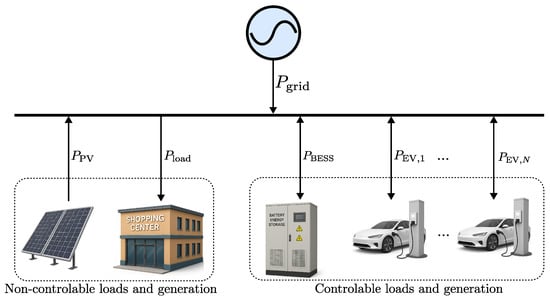
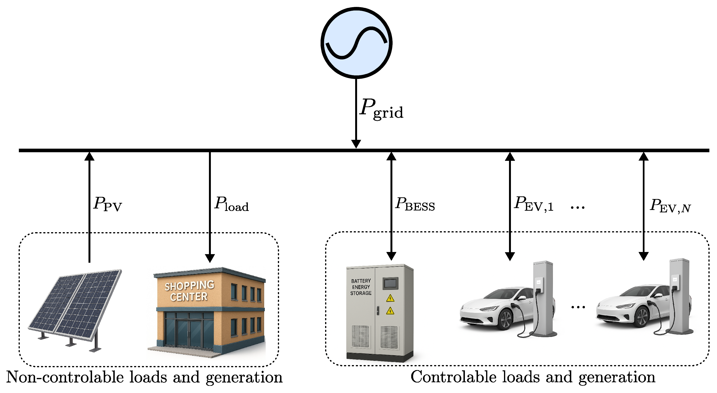
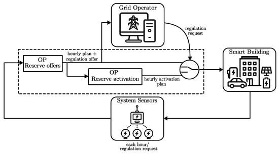
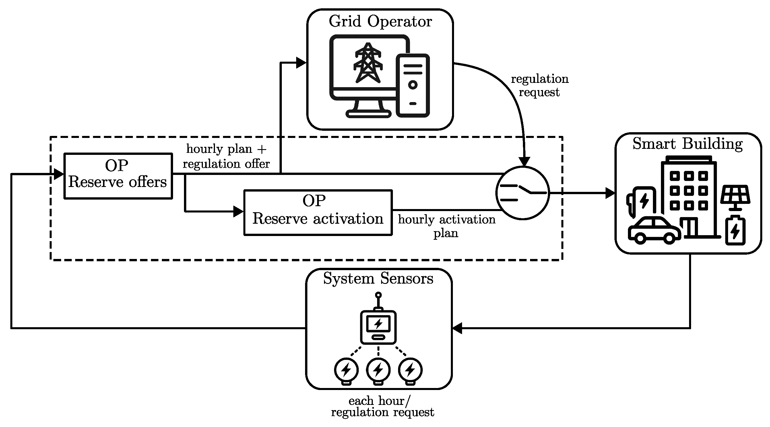
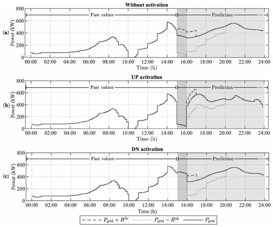
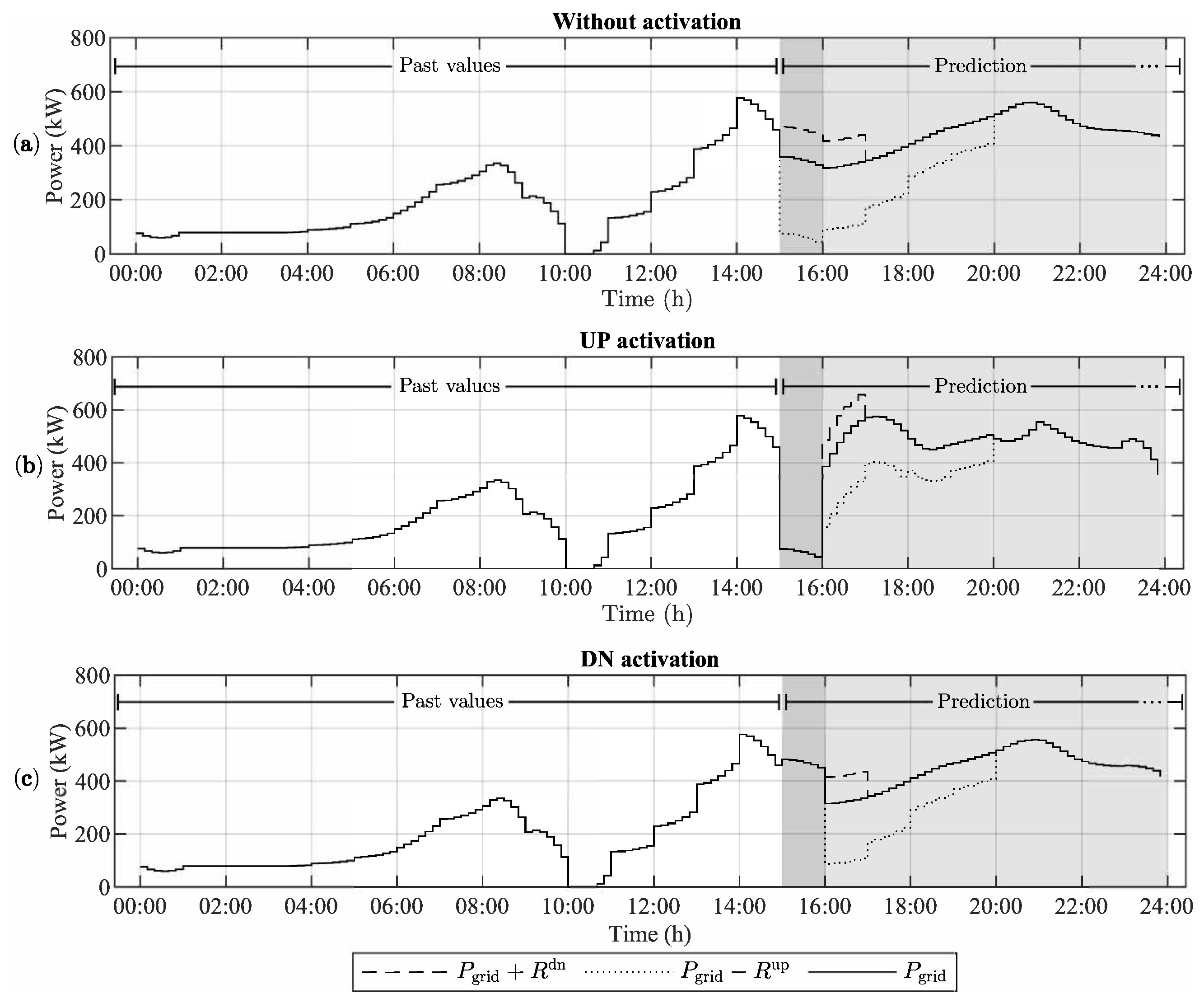
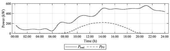
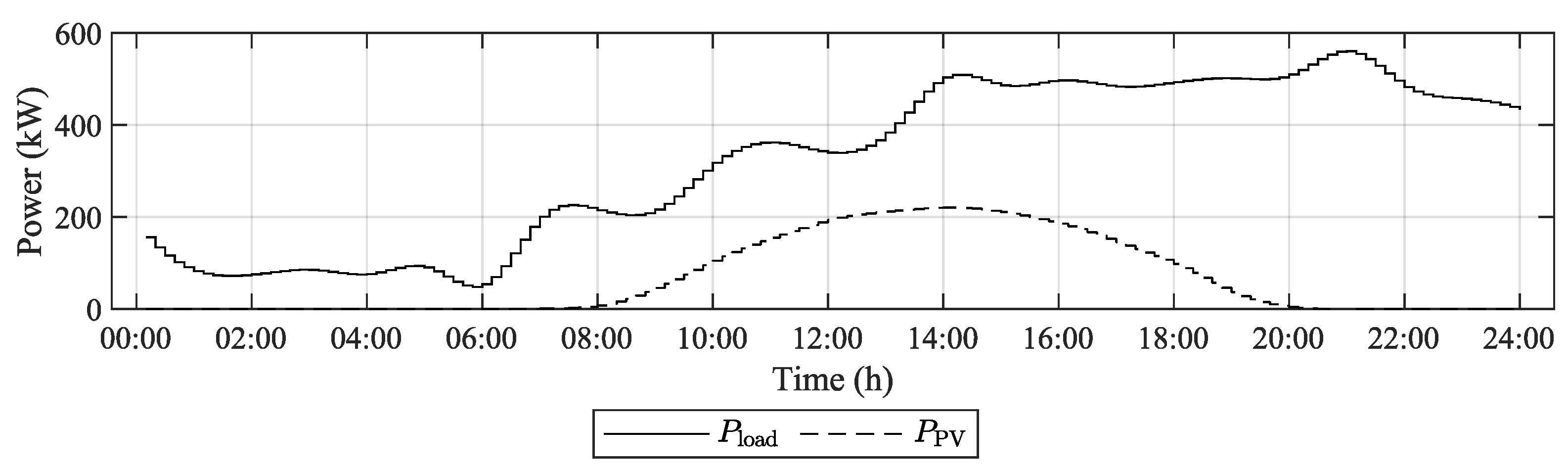
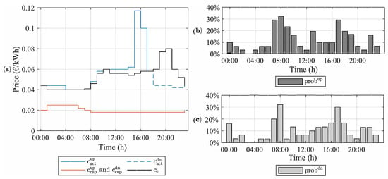
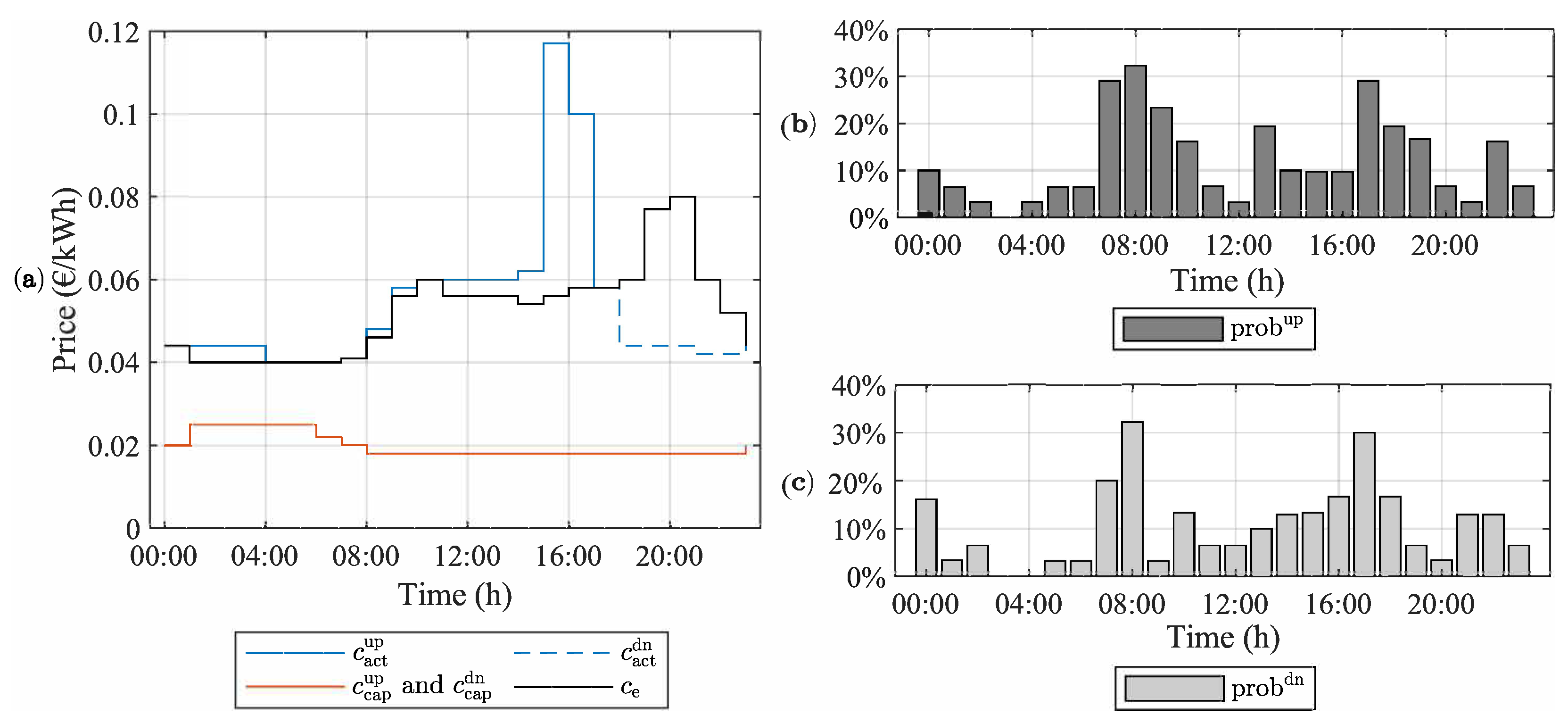
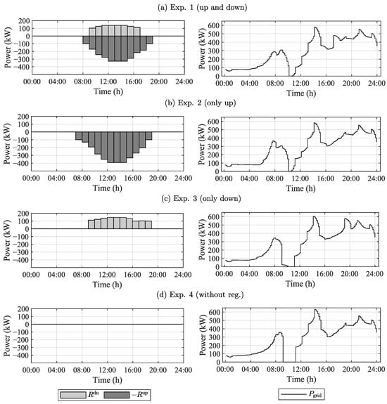
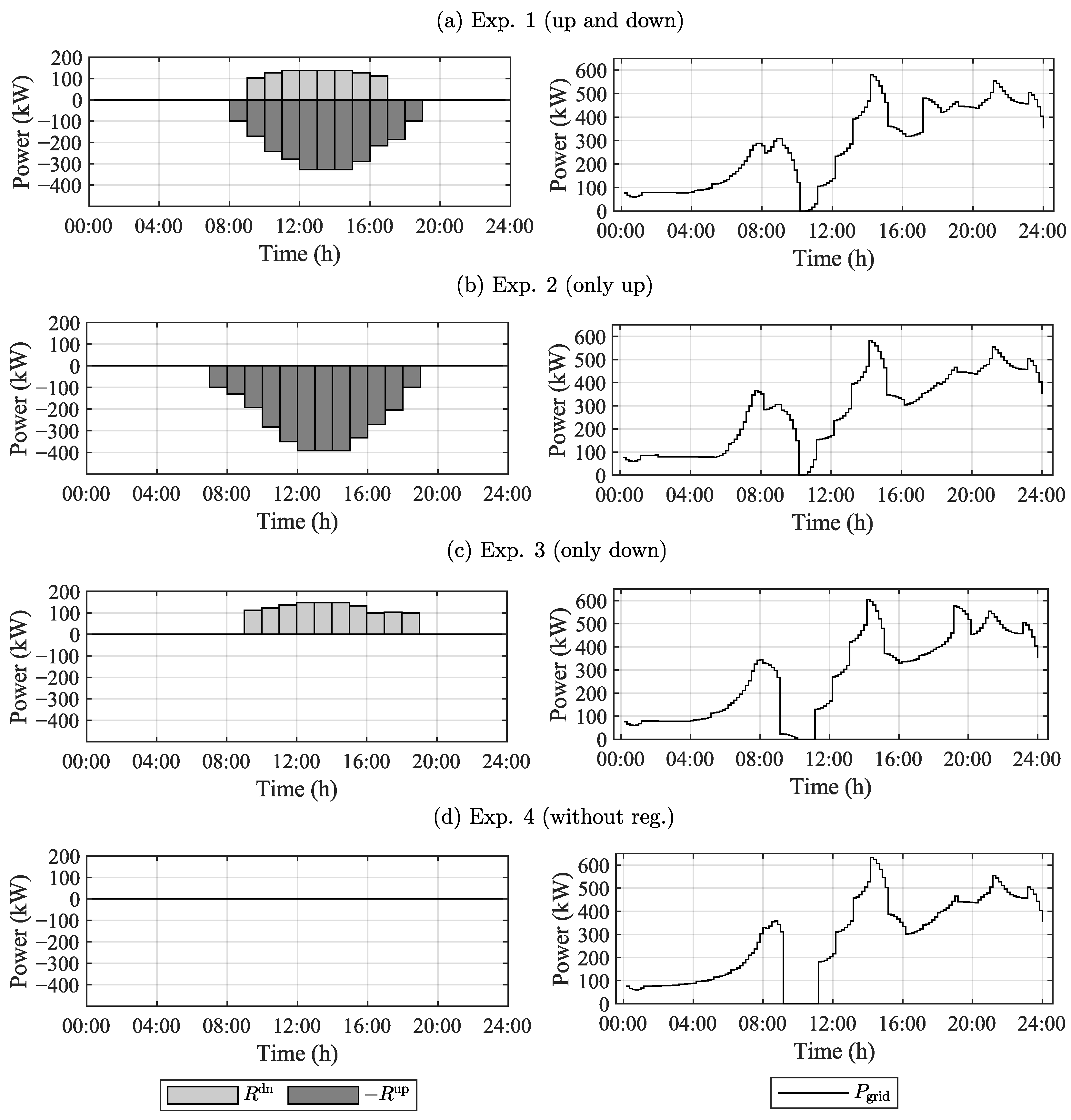
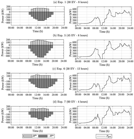
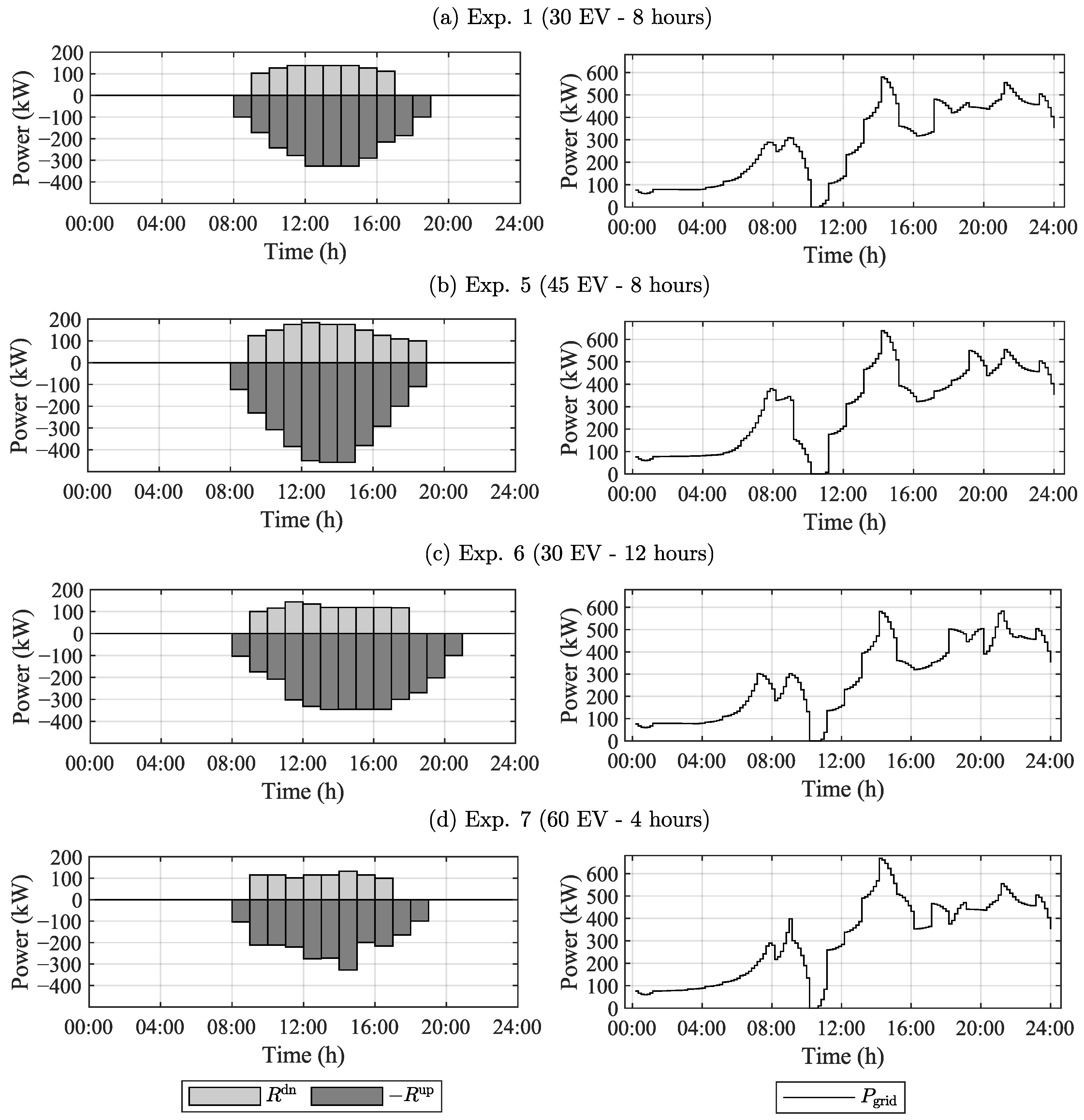
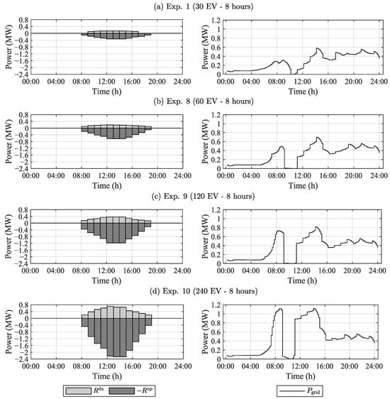
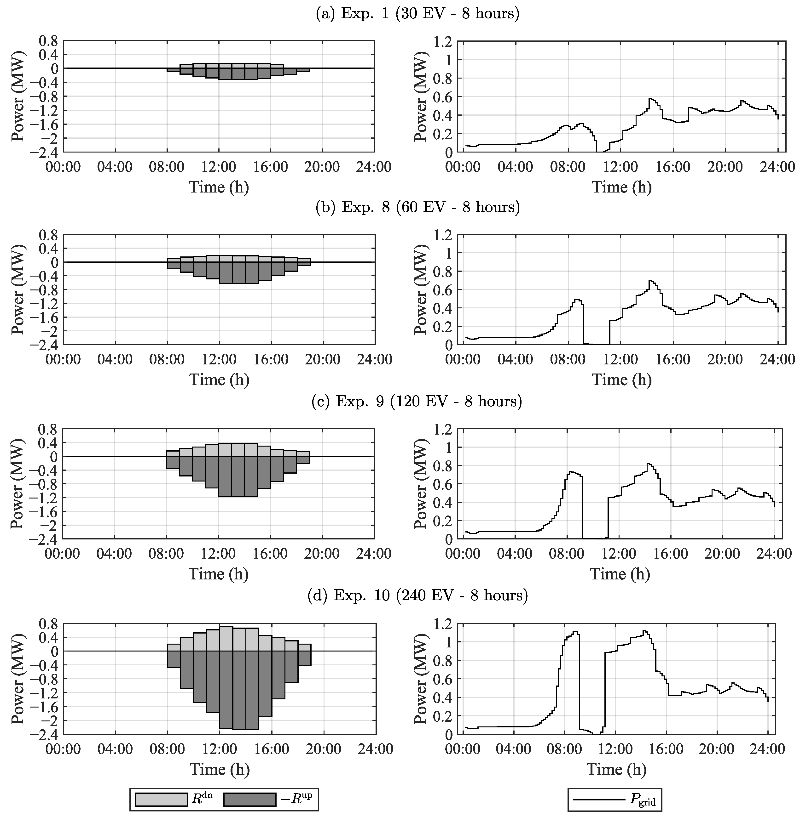
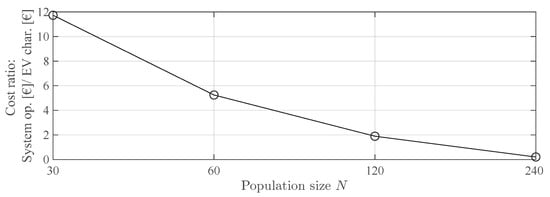
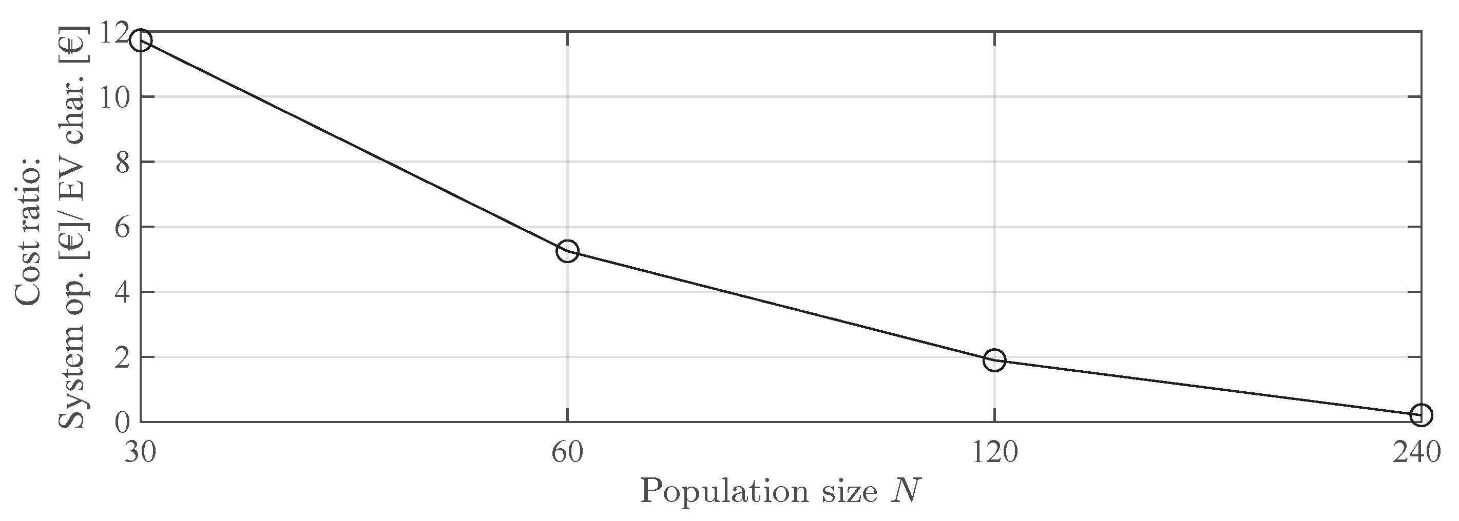

Disclaimer/Publisher’s Note: The statements, opinions and data contained in all publications are solely those of the individual author(s) and contributor(s) and not of MDPI and/or the editor(s). MDPI and/or the editor(s) disclaim responsibility for any injury to people or property resulting from any ideas, methods, instructions or products referred to in the content. |
© 2026 by the authors. Licensee MDPI, Basel, Switzerland. This article is an open access article distributed under the terms and conditions of the Creative Commons Attribution (CC BY) license.